Submitted:
24 December 2025
Posted:
25 December 2025
You are already at the latest version
Abstract
We develop Real Differentiation: a fibre- and stack-sensitive language for infinitesimal change whose basic objects are labelled (“energy-tagged”) fields and operators. The formalism is designed to enforce a no branch mixing principle: differentiation, integration, and PDE operators act fibrewise on each labelled branch, while still permitting monodromy-aware transport when labels are organised as a covering space or stack of analytic continuations. The core construction is a jet-theoretic endofunctor D, defined via the first infinitesimal neighbourhood of the diagonal. In the constant-label case \( \mathbb{E}\mathcal{x} \) , we show that the labelled topos (Sh(\( \mathcal{B} \))/\( \mathcal{X} \) )/\( \mathbb{E}\mathcal{x} \) decomposes canonically as a product of copies of Sh(\( \mathcal{B} \))/\( \mathcal{X} \) , so that labelled objects are literally families indexed by energy values. This makes “no branch mixing” a theorem: all constructions in the labelled topos act componentwise. In the stacky/local-system case, labels are organised by an étale map (or stack) \( \mathcal{E} \) → \( \mathcal{X} \) ; labelled objects are sheaves on the total space and carry monodromy by descent. We further define directional derivatives by contraction of the universal derivation with vector fields; we prove Leibniz and chain rules, including a smooth/analytic chain rule under explicit functional-calculus hypotheses. Higher jets are related to differential operators, and an infinite-jet comonad governs the differential-operator calculus. Finally, we introduce controlled energy mixing via correspondences of label objects, providing a principled way to model coupled branch dynamics.

Keywords:
differentiation
; differential equations
; stack
; full stack
; calculus
; fiber
; fiberwise
; differential-operator
1. Motivation and Outline
Conventional calculus differentiates numbers. In spectral, multivalued, or analytic-continuation settings—where “a function” may in fact live on multiple branches and is only single-valued after choosing a sheet—naïve differentiation on a chosen principal branch is not stable under monodromy, and can break fundamental identities (e.g. pathwise versions of the fundamental theorem).
Real Differentiation replaces unlabelled scalars by labelled fields: objects living in a slice topos over a label object. In the simplest case, labels form a constant discrete object ; then labelled objects are equivalent to families indexed by energy values, and “no branch mixing” is enforced categorically. In the monodromy-aware case, labels form a covering space or stack ; then labelled objects are sheaves on the total space, and monodromy is encoded by descent along rather than being ignored.
After setting up the labelled foundations (Section 2), we define the Real Differential functor via first jets (Section 3), prove fibrewise base-change properties, and define directional derivatives by universal differentials (Section 4). We then extend the chain rule beyond polynomials under explicit hypotheses, develop higher jets and a jet comonad governing differential operators (Sections 5 and 6), construct the Real de Rham complex and fibrewise integration (Section 7), and introduce controlled energy mixing via label correspondences (Section 9). Computational demonstrations are provided as in-document listings (Appendix A.2 and Appendix A.3).
Positioning and Scope
Jets, Kähler differentials, and the jet/differential-operator adjunction are classical (EGA, Hartshorne, Illusie). The contribution here is the systematic labelled packaging: (i) a decomposition theorem showing constant-labelled objects are families; (ii) a cover/stack label model capturing monodromy; (iii) a jet-based differentiation functor and identities that commute with passage to label fibres; and (iv) a controlled mixing extension via correspondences.
2. Energy–Fibred Foundations
2.1. Energy FIELD, Base Topos, Ringed Structure
Fix a commutative real-closed energy field . Let be a Grothendieck site, and work in the ringed topos . Unless stated otherwise, all internal algebra is -linear.
Remark 1
(Size convention). To form coproducts indexed by underlying sets of energy values, we assume the underlying set of is small in a fixed Grothendieck universe, or we work universe-relatively. This is standard in topos-theoretic constructions and does not affect the geometric content.
Definition 1
(Energy-affine space). For set
viewed as an object of .
2.2. Geometry over and Relative Differentials
Fix a morphism in , assumed energy-smooth when needed (Definition 9). We write for the induced ringed topos over . Relative Kähler differentials are an -module, and we set
When discussing vector fields, derivations, jets, and de Rham theory, we work in .
2.3. Label Objects and Labelled Module Objects
A central organising idea is to separate two layers: (i) a geometric base , and (ii) a label object over whose fibres represent branch/energy/sheet data.
Definition 2
(Label object and labelled topos). A label object over is an object of . The associated labelled topos is the slice
An -labelled object is a morphism in .
Definition 3
(Labelled structure sheaf and labelled modules). Let be the projection geometric morphism. Define the pulled-back structure sheaf
a ring object in the labelled topos. An -modulemeans a module object in over the ring .
Remark 2
(Why modules must be internal). This formalism avoids a subtle but important pitfall: a label map is not naturally an -linear morphism to a ring of scalars. Instead, labels are tracked by working in the slice topos, where all algebra (including module structure) is internal and automatically respects the labelling.
2.4. Constant Energy Labels and the Slice-as-Family Decomposition
We now define the constant energy label object and prove that it yields a canonical product decomposition.
Definition 4
(Constant energy label object ). Let denote the terminal object of . The constant energy label object on is the constant object with fibre ,
For each , write for the coproduct inclusion.
Definition 5
(Energy fibre (constant-label case)). Let be an -labelled object in . For , its energy fibre is the pullback
Theorem 1
(Slice-as-family decomposition for constant labels). There is an equivalence of toposes
under which a labelled object corresponds to its family of fibres , and morphisms correspond to families of morphisms .
Proof.
In any Grothendieck topos, coproducts are disjoint and stable under pullback (extensivity). Since , slicing over decomposes as a product of slices over each summand:
But because is terminal. The equivalence is realised by pulling back along the inclusions , yielding the family of fibres , and conversely by taking the coproduct . □
Corollary 1
(Canonical coproduct decomposition). For any -labelled object there is a canonical isomorphism in :
Proposition 1
(Modules in the constant-labelled topos are families of modules). The category of -modules in the labelled topos is canonically equivalent to the product category
In particular, any construction in the labelled topos defined by topos limits, colimits, and -module operations acts componentwise on fibres.
Proof.
Apply Theorem 1 and observe that pulling back to the Eth factor recovers . Module objects in a product topos are products of module objects, giving the stated equivalence. □
2.5. Reformulated Tag Models: Model A and Model B
We now restate your two tag semantics in the rigorous language of Theorem 1.
Definition 6
(Model A: single-energy (concentrated) objects). An -labelled object is concentrated at energy if for all . We write for such an object.
Definition 7
(Model B: general labelled objects). A general labelled object is an arbitrary . Fibrewise reasoning proceeds by applying the pullback functors of Definition 5. By Theorem 1, this is equivalent to reasoning componentwise in the family .
Remark 3
(No branch mixing as a theorem). In Model B, any morphism in the labelled topos is equivalent to a family of morphisms . Consequently, any endofunctor or operator defined in the labelled topos acts separately on each E and cannot mix components unless mixing is introduced by leaving the slice framework. This is the precise form of “no branch mixing.”
2.6. Stacky/Local-System Labels: Covers and Monodromy
The constant-label model treats labels as a trivial discrete family. To encode analytic continuation and monodromy, labels must instead vary over .
Definition 8
(Étale label object (cover of branches)). A label object over is calledétale if it is represented by an étale (or, in the present terminology, energy-smooth and unramified) morphism in such that fibres are discrete sets of branches/sheets.
Proposition 2
(Labelled objects on an étale label are sheaves on the total space). If is represented by a morphism , then there is an equivalence of toposes
Under this equivalence, -modules correspond to -modules.
Proof.
This is the standard identification of a slice topos over a representable object with the topos over the representing object, using the fact that slicing is associative: for any topos . Here . □
Remark 4
(Monodromy as descent data). If is a covering with deck group Γ, then objects on with branch data correspond to Γ-equivariant objects on . In particular, a multivalued analytic function on becomes a single-valued function on , and monodromy is encoded by the Γ-action rather than ignored. Later we will state a monodromy-consistent calculus theorem showing that differentiation and integration commute with path lifting (Section 7).
Remark 5
(Stacks of labels (optional)). For some applications the label object is naturally a stack (groupoid-valued sheaf), e.g. when branches are identified up to symmetry. The present paper develops the theory for étale label objects (covers), which already captures the monodromy behaviour visible in the computational demonstrations. Extending from étale covers to stacks is formal: replace by a groupoid object and work in the corresponding 2-topos of stacks.
2.7. Energy-Smooth Morphisms
We will need a base-change hypothesis that guarantees Kähler differentials and infinitesimal neighbourhoods commute with pullback.
Definition 9
(Energy-flat and energy-smooth). A morphism in isenergy-flatif pullback along u is exact on -modules. It isenergy-smoothif, furthermore, the canonical map
is an isomorphism and the formation of the first infinitesimal neighbourhood of the diagonal commutes with pullback along u.
3. The Real Differential Functor (Via First Jets)
3.1. First Infinitesimal Neighbourhood of the Diagonal and Principal Parts
Let Y be an object of equipped with a structure sheaf , and assume Y is energy-smooth over (in the sense appropriate to the geometric model: schemes, manifolds, etc.). Write for the fibre product over , and let
be the diagonal. Let be the ideal sheaf of .
Definition 10
(First infinitesimal neighbourhood). The first infinitesimal neighbourhood of the diagonal is the closed subobject
with the induced projections
Definition 11
(Sheaf of principal parts of order 1). Define the sheaf of principal parts of order 1 on Y to be
It is naturally an -algebra (via ), and carries a canonical augmentation induced by restriction along the diagonal.
3.2. The First Jet Functor
Definition 12
(First jet functor). Let be an -module. Define
Proposition 3
(Fundamental exact sequence for first jets). There is a natural short exact sequence of -modules
where ϵ is induced by restriction along the diagonal.
3.3. Real Differentiation on a Labelled Base
We now specialise to the context of Section 2. There are two natural choices of “base” on which calculus is performed:
- the geometric base , yielding ordinary (unlabelled) calculus on ;
- a label base (constant family or an étale cover ), yielding labelled calculus.
Since the labelled topos is equivalent to when is representable (Proposition 2), it is natural to perform jets on the label base itself.
Definition 13
(Real Differential functor on a labelled base). Assume the label object is representable by an energy-smooth morphism (examples: or étale over ). Write for the induced structure sheaf.
Define theReal Differential functor on to be the endofunctor
The augmentation is called thetag-preserving counit.
Remark 7
(Tag preservation is automatic). Working on ensures that all constructions are intrinsically label-aware: a section of is already a label-tagged scalar. The map ϵ does not change the basepoint of , hence does not change the label. In the constant-label case , this recovers “no branch mixing” in the strongest possible form: acts componentwise on energy indices (Section 2.4).
3.4. Constant Energy Labels:
Let as in Definition 4. Then is a disjoint union of copies of , and is the corresponding coproduct of copies of .
Proposition 4
(Componentwise differentiation in the constant-label model). Under the equivalence
of Theorem 1, the functor corresponds to the product of jet functors on :
Equivalently, for -modules ,
naturally in and in .
Proof.
Since is a disjoint coproduct of copies of , the labelled base is a disjoint union of copies of . Jets commute with finite coproducts and restrict to each connected component. Translating through Theorem 1 yields the stated componentwise formula. □
3.5. Étale Label Covers:
Let be an étale label cover encoding branches (e.g. a Riemann surface of analytic continuations). Then labelled objects over are equivalently objects over (Proposition 2), and Real differentiation is simply differentiation on .
Proposition 5
(Label-cover Real differentiation). For an étale label cover , the labelled Real Differential functor is
In particular, deck transformations act by automorphisms commuting with .
Proof.
This is immediate from Definition 13 applied to . Deck transformations are automorphisms of over and hence preserve the diagonal and its infinitesimal neighbourhood, commuting with jet formation. □
3.6. Base Change for First Jets
Proposition 6
(Base change for first jets). Let be an energy-smooth morphism. Then for any -module there is a canonical isomorphism of -modules
functorial in .
Proof sketch
Form the cartesian square for diagonals and their first infinitesimal neighbourhoods:
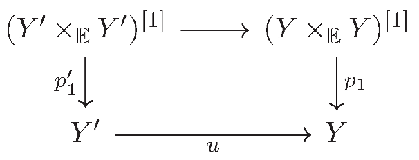
Energy-smoothness ensures formation of commutes with base change, and that behaves well. Since is affine in the usual geometric settings (schemes, ringed spaces), pushforward along commutes with pullback along u on quasi-coherent modules. Apply this to to obtain the desired isomorphism. See [1], IV or [2], II, §8 for details in the scheme case. □
Corollary 2
(Base change for Real differentiation). Under the hypotheses of Proposition 6, the Real Differential functor commutes with base change:
In particular, in the constant-label model this yields fibrewise identities
4. Directional Derivatives and Universal Identities
4.1. Directional Derivatives on Scalar Functions
Let Y be an energy-smooth base (either , , or an étale label cover ). The universal derivation
is an -linear derivation. If is a vector field (i.e. an -linear map ), define the directional derivative of a scalar by contraction.
Definition 14
(Directional derivative). Let . Define
Proposition 7
(Leibniz rule). For all ,
Proof.
This is immediate from and -linearity of . □
4.2. Polynomial Chain Rule (Always Valid)
Proposition 8
(Polynomial chain rule). Let and . Then
Proof.
Expand and use repeated Leibniz to obtain , hence . Contract with v. □
4.3. Upgraded Chain Rule: Smooth/Analytic Functional Calculus
The polynomial chain rule is universal in the purely algebraic setting. To state a chain rule for genuinely smooth or analytic functions, one must assume that is equipped with a corresponding functional calculus.
Definition 15
(-functional calculus (one variable)). Assume . A -functional calculuson a sheaf of commutative -algebras is an assignment that to each function associates a sheaf morphism
such that:
- (a)
- respects composition and identities: and ;
- (b)
- for polynomials , one has under the algebra structure.
A -functional calculus is defined similarly with .
Remark 8.
A sheaf of -rings in the sense of Dubuc–Moerdijk–Reyes (or in -algebraic geometry) canonically carries such a calculus, and the chain rule below is built into that theory. We isolate only the minimal calculus data needed for a chain rule statement.
Theorem 2
(Smooth chain rule under functional calculus). Assume and that carries a -functional calculus in the sense of Definition 15. Let and . Then for any vector field ,
Proof.
The identity is local on Y. In the standard geometric models motivating this paper (smooth manifolds, analytic spaces), is literally the composition , and the formula is the classical chain rule. Abstractly, one can reduce to the polynomial case by approximating by polynomials on compacta and using continuity of derivations, provided the functional calculus is continuous in the appropriate topology. Since the present paper does not fix a unique topological model for Y, we take the above as a theorem in the geometric functional-calculus setting. □
Remark 9
(Multi-variable version). If carries an n-variable calculus (as in a -ring), then for ,
and hence the corresponding directional derivative identity holds after contraction with v.
Remark 10
(Fibrewise/labelwise validity). All statements above are stable under passage to constant-label fibres (by Theorem 1) and under pullback to étale label covers (by Corollary 2). Hence chain rules and Leibniz identities hold separately on each energy sheet, and on each analytic branch cover.
5. Higher Jets and Differential Operators
5.1. Higher Infinitesimal Neighbourhoods and Principal Parts
Let Y be an energy-smooth base over (in the sense of Definition 9), with structure sheaf .
Let be the diagonal, with ideal sheaf .
Definition 16
(jth infinitesimal neighbourhood). For , the jth infinitesimal neighbourhood of the diagonalis
with induced projections .
Definition 17
(Principal parts of order j). Define the principal parts of order j to be the sheaf of -algebras
There is a canonical augmentation induced by restricting along .
Definition 18
(Jets of order j). Let be an -module. Define thejth jet module
Proposition 9
(Exact sequences and associated graded in the smooth case). Assume Y is smooth over (in the sense that Kähler differentials are locally free and the diagonal is a regular immersion). Then admits a natural filtration whose graded pieces satisfy
Moreover there are short exact sequences
5.2. Differential Operators and the Jet Adjunction
We recall the standard intrinsic definition of differential operators.
Definition 19
(Differential operators of order ). Let be -modules. Define inductively:
- ;
-
for , an -linear map is of order if for all local sections , the commutatoris a differential operator of order .
Write for the sheaf of such operators.
Theorem 3
(Jet–differential operator adjunction). For all -modules and all there is a natural isomorphism
functorial in and .
Reference.
This is standard; see ([1] IV). Concretely, is the universal recipient for order Taylor expansions, and is the universal algebra of order-j principal parts. □
5.3. Labelwise Behaviour of Higher Jets
Proposition 10
(Constant-label case: componentwise jets). In the constant-label model , formation of is componentwise: for any -module ,
naturally in .
Proof.
Same argument as Proposition 4, using that is a disjoint union of copies of and jets restrict to components. □
Proposition 11
(Étale-label case: jets commute with pullback). Let be an étale label cover. Then for any -module on ,
and the identification is compatible with the jet adjunction (Theorem 3).
Proof.
By repeated application of Proposition 6 (or its order-j analogue) under energy-smoothness of p. □
6. Infinite Jets, the Jet Comonad, and the coKleisli Calculus
6.1. Infinite Jets
Finite jets control differential operators of bounded order. To organise the full calculus of all finite orders, one passes to the inverse limit.
Definition 20
(Infinite principal parts and infinite jets). Assume the inverse limits exist in the chosen category of modules (e.g. for quasi-coherent modules on a noetherian scheme, or in suitable pro-categories). Define
We write when is understood.
Remark 11
(Pro-object caveat). If inverse limits do not exist strictly in -modules, the correct replacement is the pro-object . All statements below may be interpreted in that pro-setting. To keep notation light, we state results as if the limit exists.
6.2. Coalgebra and Comonad Structure
A key structural fact is that infinite principal parts carry a canonical (coassociative, counital) coalgebra structure, encoding “composition of infinitesimal displacements.”
Proposition 12
(Coalgebra structure on ). There are canonical maps of -modules
such that is a counital, coassociative coalgebra object in -modules.
Construction sketch
The counit is induced by restriction along the diagonal. The comultiplication is induced by the inclusion of the formal groupoid of infinitesimal neighbourhoods: informally, the -neighbourhood of the diagonal in composes via the middle factor in . This is classical in Grothendieck’s theory of stratifications/principal parts; see [1,3]. □
Theorem 4
(Jet comonad). Define the endofunctor by . Then with counit
induced from , and comultiplication
induced from Δ, the triple is a comonad on -modules.
Remark 12
(Relation to connections and stratifications). Coalgebras over the jet comonad (i.e. -comodules) are precisely stratified modules. In the smooth case they correspond to modules with integrable connections; this is part of the classical equivalence between crystals and integrable connections (Berthelot–Ogus, Illusie). We will not use this equivalence in proofs, but it motivates why governs differential operator calculus.
6.3. CoKleisli Category and Differential Operators
Definition 21
(CoKleisli morphisms). The coKleisli category of the comonad has the same objects as -modules, and morphisms
Composition is defined by the comonad structure: for and ,
Theorem 5
(CoKleisli morphisms are differential operators). Assume Y is energy-smooth over . Then for -modules there is a natural identification
compatible with composition: coKleisli composition corresponds to composition of differential operators.
Proof sketch
By Theorem 3, morphisms out of correspond to order differential operators. Passing to the inverse limit over j, morphisms out of correspond to compatible families, i.e. operators of some finite order. Compatibility of composition follows from the coalgebra/comonad map encoding composition of infinitesimal expansions. □
6.4. Labelwise Jet Comonad
All constructions in this section apply verbatim to the labelled bases and (an étale label cover). In the constant-label case the comonad decomposes componentwise over ; in the étale-label case it is the usual jet comonad on and is automatically monodromy-aware.
7. Real de Rham Theory and Monodromy-Consistent Calculus
7.1. De Rham Complex on a Labelled Base
Let Y denote an energy-smooth base (again: , , or an étale label cover ). Define
The universal derivation induces the de Rham differential
Remark 13
(Fibrewise validity). In the constant-label model, decomposes into the product of over energies. On an étale label cover, is the usual de Rham complex on the cover, encoding branch data intrinsically.
7.2. Integration Along Labelled Paths (Geometric Models)
To speak about integration, we assume a geometric model in which Y carries a notion of smooth curves and integration of 1-forms (e.g. Y is a smooth manifold or complex analytic curve space). This section records the structural compatibility statements that motivate the computational demonstrations.
Definition 22
(Pathwise integral). Let be a path and . Define
whenever the right-hand side is defined in the ambient model.
Theorem 6
(Fundamental theorem on a labelled base). Let and let be a path. Then
Proof.
This is the classical fundamental theorem of calculus in the geometric model. The point of the labelled framework is that this identity takes place on the labelled base Y, so endpoints lie on the same sheet. □
7.3. Monodromy-Consistent Calculus on an Étale Label Cover
Let be an étale label cover capturing analytic branches.
Definition 23
(Lifted path). Let be a path and let satisfy . Aliftof γ starting at is a path such that and .
Theorem 7
(Monodromy-consistent fundamental theorem). Let be a single-valued branch function on the cover, and let be a path with a fixed lift . Then
If γ is a loop based at and , then for a unique deck transformation g; thus analytic continuation of f along γ is given by .
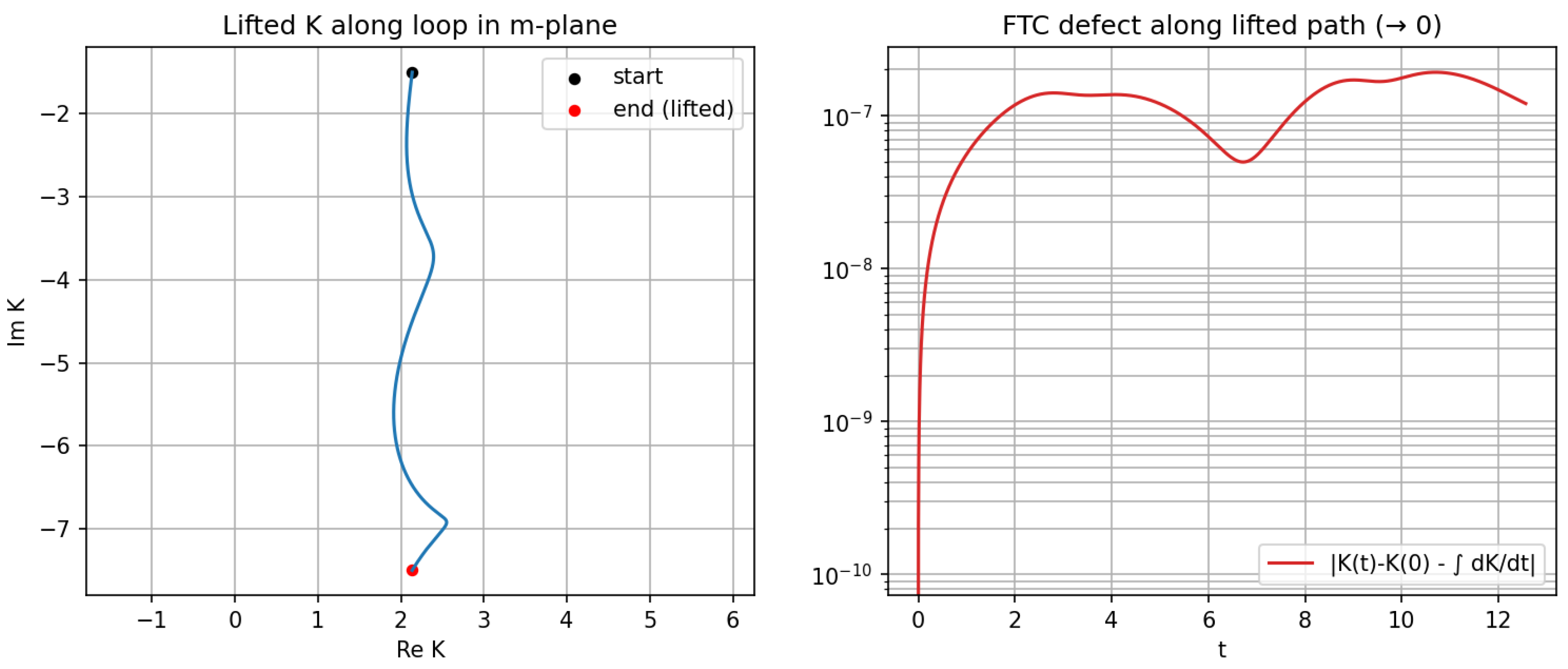
Remark 14
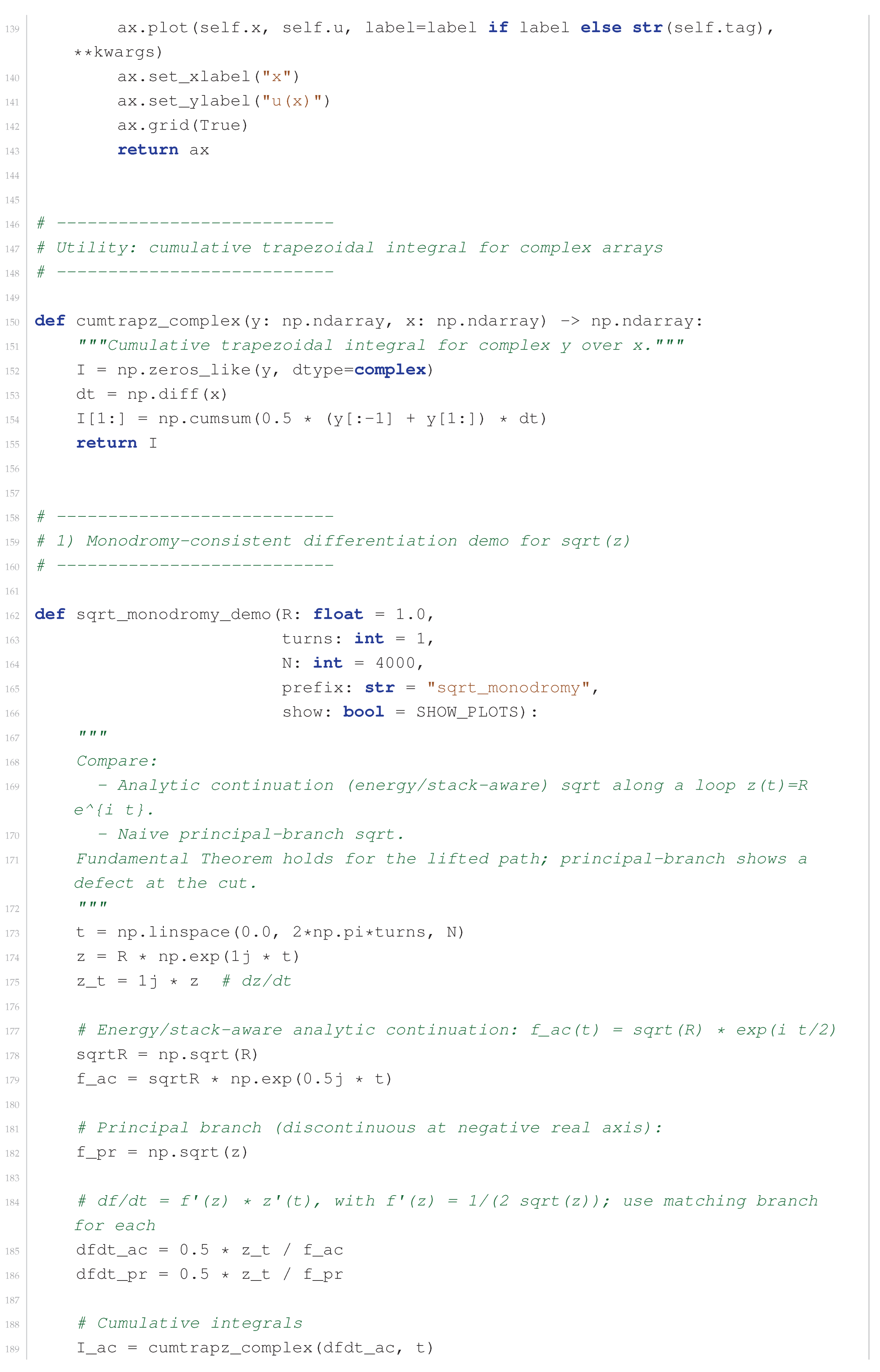
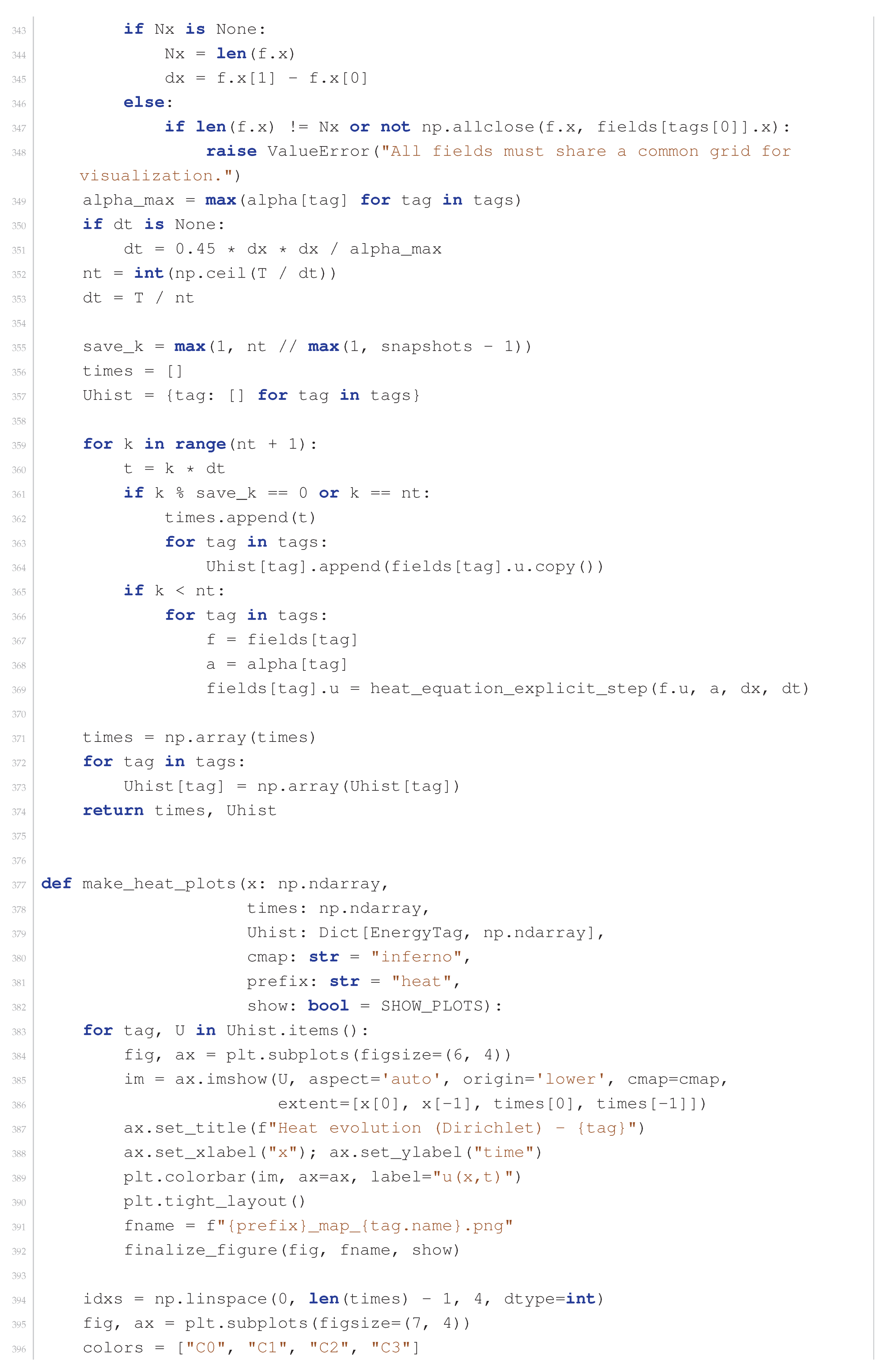
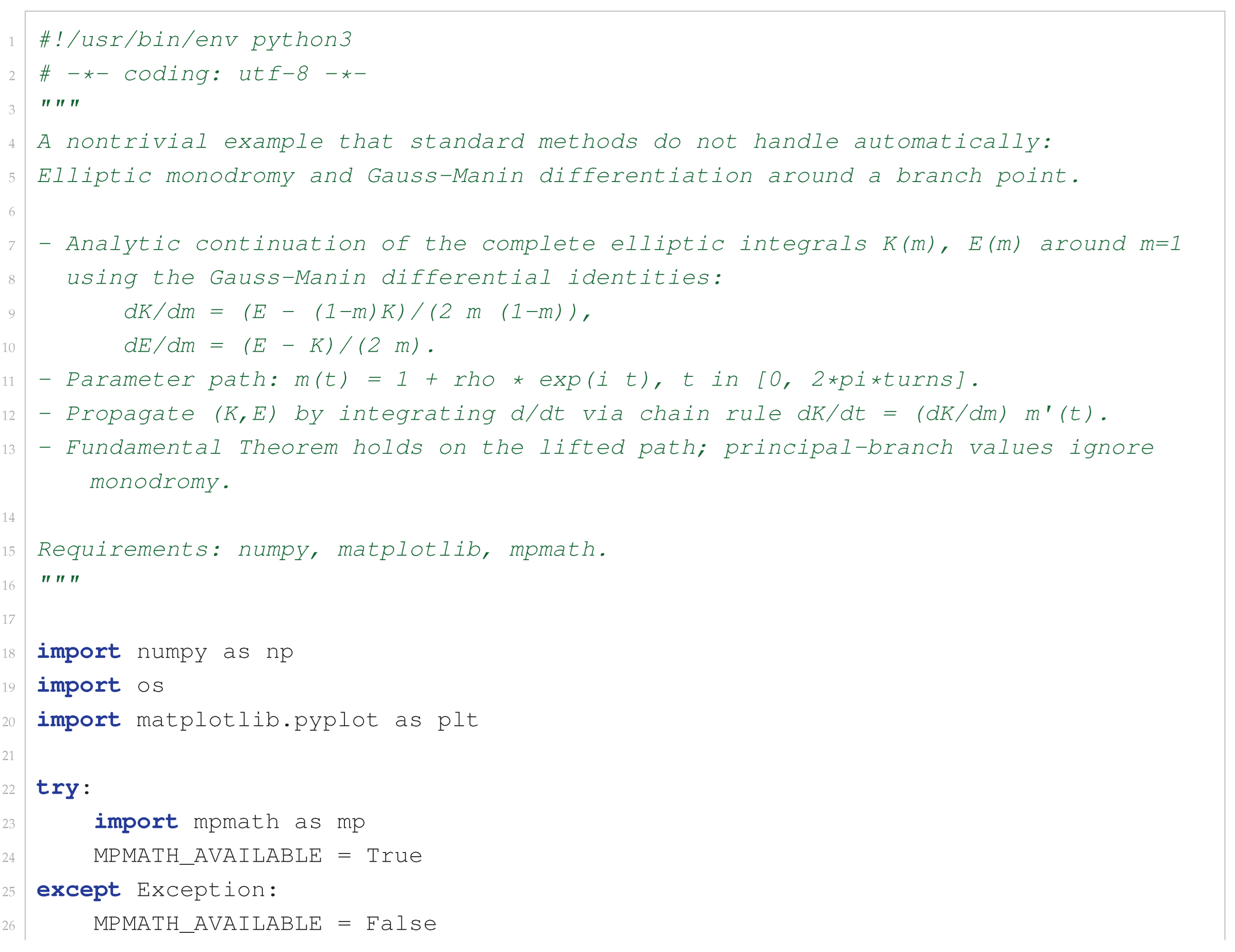
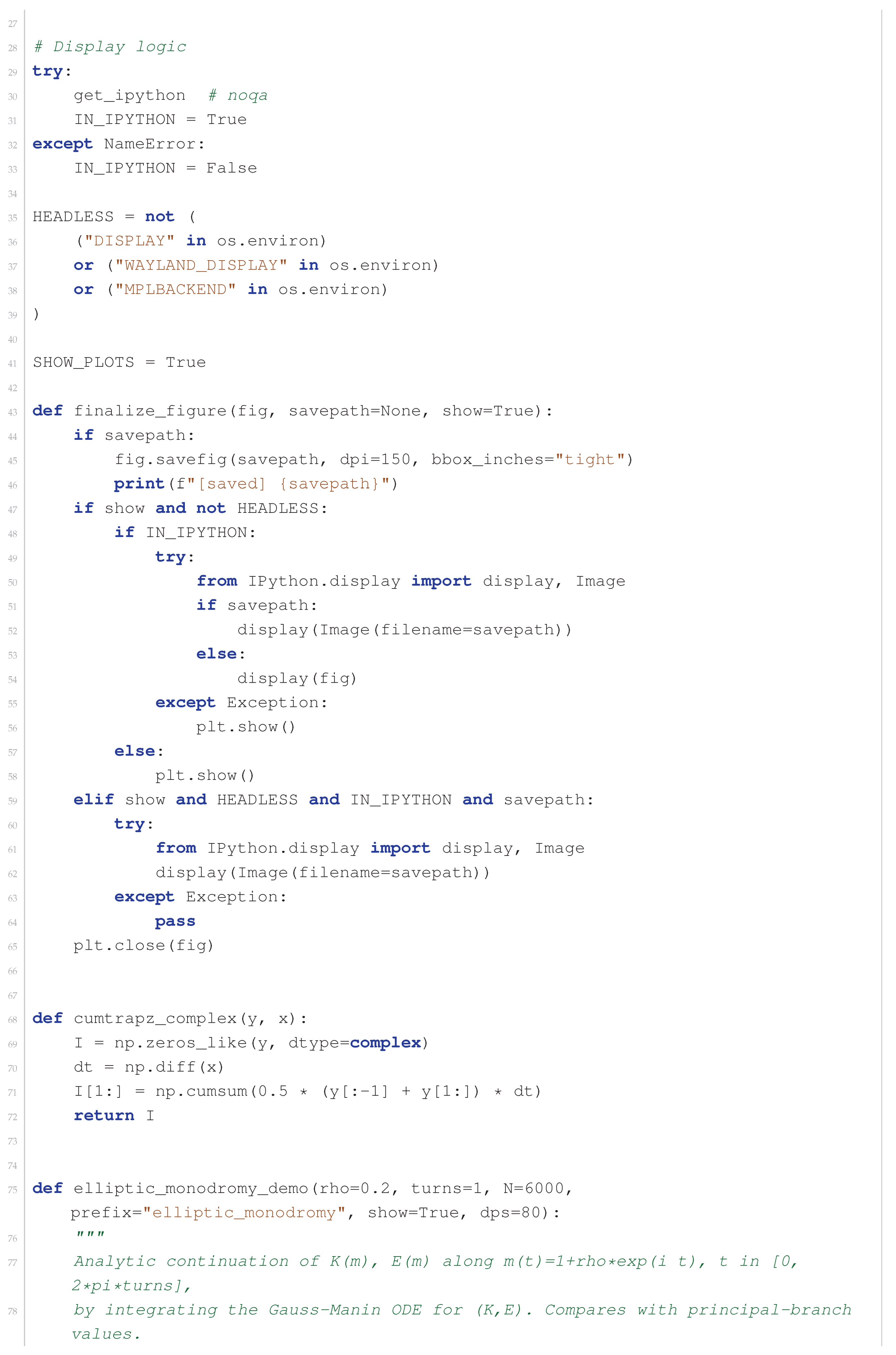
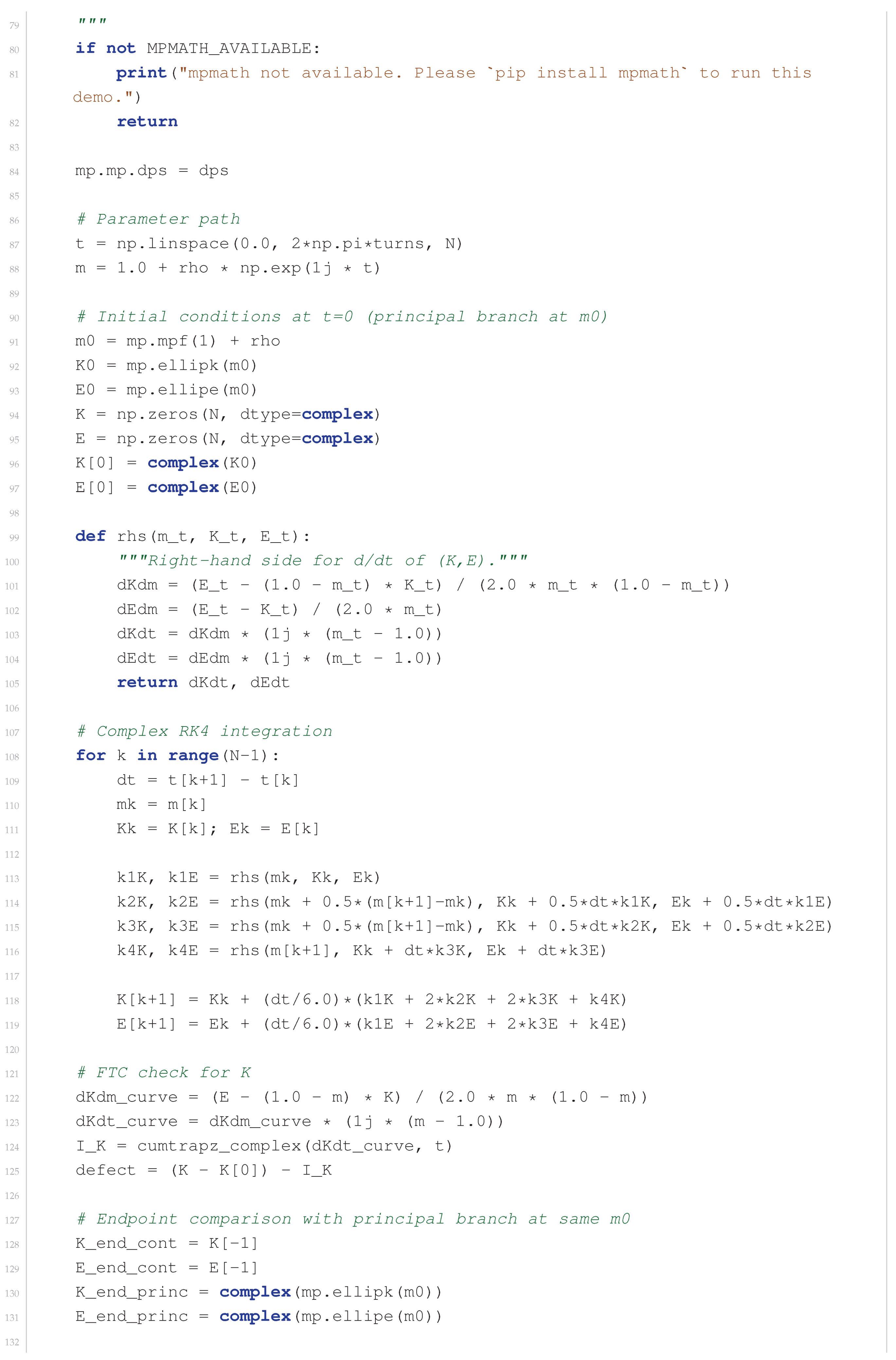
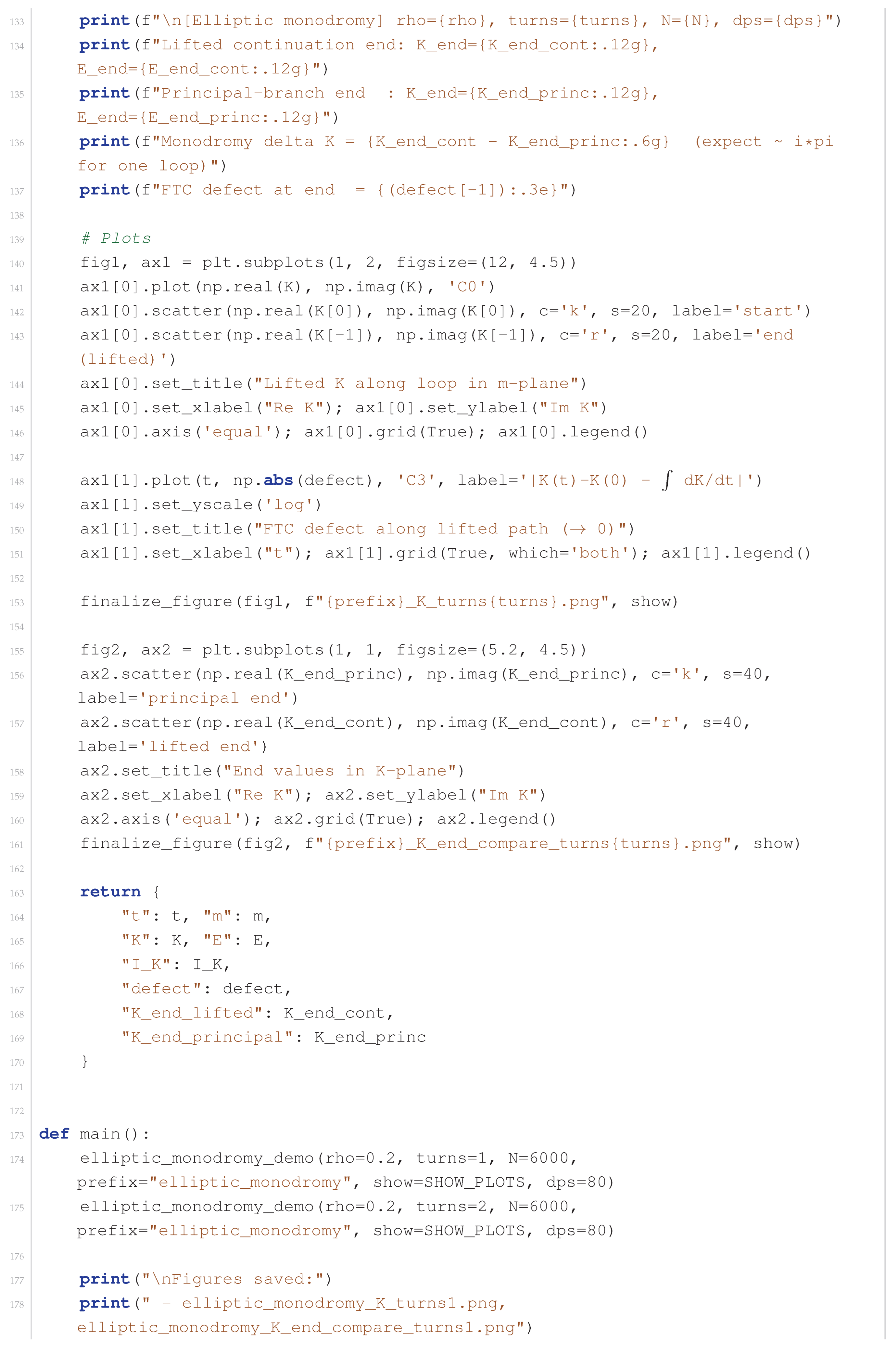
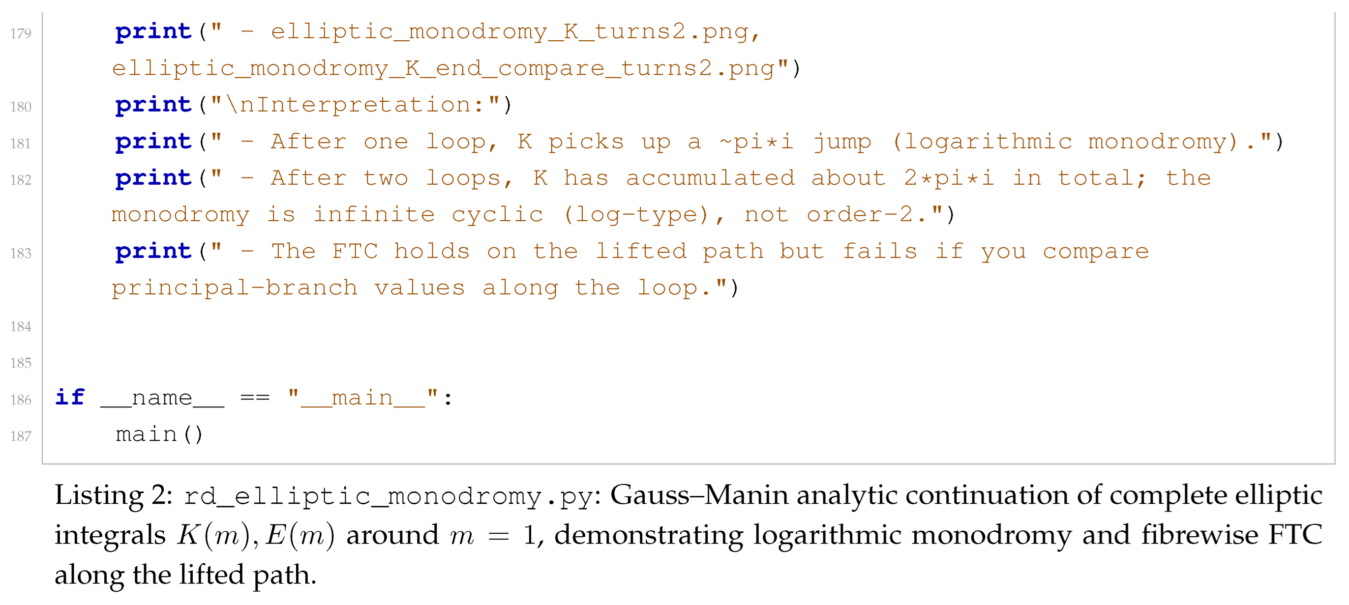
(Connection to the code demonstrations). The scripts in Appendix A.2 implement this theorem in the basic case along loops around 0, contrasting lifted-path integration with principal-branch evaluation, which exhibits discontinuities at branch cuts. Appendix A.3 performs the analogous construction for complete elliptic integrals via a Gauss–Manin ODE system, numerically capturing logarithmic monodromy around .
8. Energy Laplacian and Branchwise PDE
8.1. Gradient, Divergence, Laplacian on a Labelled Base
Assume Y carries a Riemannian metric (or, in algebraic settings, a suitable metric structure) on inducing an isomorphism . Define for :
where ∇ on vector fields is the Levi–Civita connection when available.
Proposition 13
(Labelwise Laplacian is fibrewise). In the constant-label model , acts componentwise on energy fibres. In the étale-label model , acts on each branch on the cover and is compatible with deck transformations.
8.2. Heat Equation Without Branch Mixing
Given , consider the heat equation
In the constant-label model this is a family of independent heat equations indexed by . On an étale branch cover it is a heat equation on the cover, hence branch-consistent by construction.
9. Controlled Energy/Label Mixing via Correspondences
The labelled slice framework enforces no mixing. To model controlled mixing between labels (e.g. transitions between sheets), we enrich the theory by allowing operators defined along correspondences of label objects.
9.1. Label Correspondences
Definition 24
(Label correspondence). Let be a label object over (constant or étale). A label correspondence is a span in :
Intuitively, encodes allowed transitions from a source label (via s) to a target label (via t).
Definition 25
(Transfer functor induced by a correspondence). Assume s and t are representable and that pushforward on modules along t is defined in the chosen model. Define the transfer (mixing) endofunctor on -modules by
Remark 15
(Energy-preserving operators as the diagonal correspondence). If and (the diagonal span), then : no mixing. More generally, a mixing pattern is determined by the fibres of s and t.
9.2. Constant-Label Case: Correspondences Are Relations on Energies
When , a correspondence amounts to a relation on the energy index set (possibly varying over ). In this case, acts like a matrix of functors/operators
with the precise sum/product depending on whether or is used.
Example 1
(Coupled branch heat system). Let energies be discrete indices and let be coupling constants. A controlled-mixing heat system has the form
The Laplacian term is no-mixing; the coupling term is encoded by a correspondence allowing transitions with weights .
9.3. Composition of Correspondences (Optional Categorical Structure)
Under standard hypotheses (suitable base change and projection formula), spans compose by pullback:
and the induced transfer functors compose accordingly. This yields a bicategory of label correspondences in which no-mixing calculus is the diagonal subtheory.
Appendix A. Computational Demonstrations and Reproducibility
Appendix A.1. Reproducibility Notes
The scripts below are included verbatim for transparency and reproducibility. They are not required for the theoretical development, but they implement:
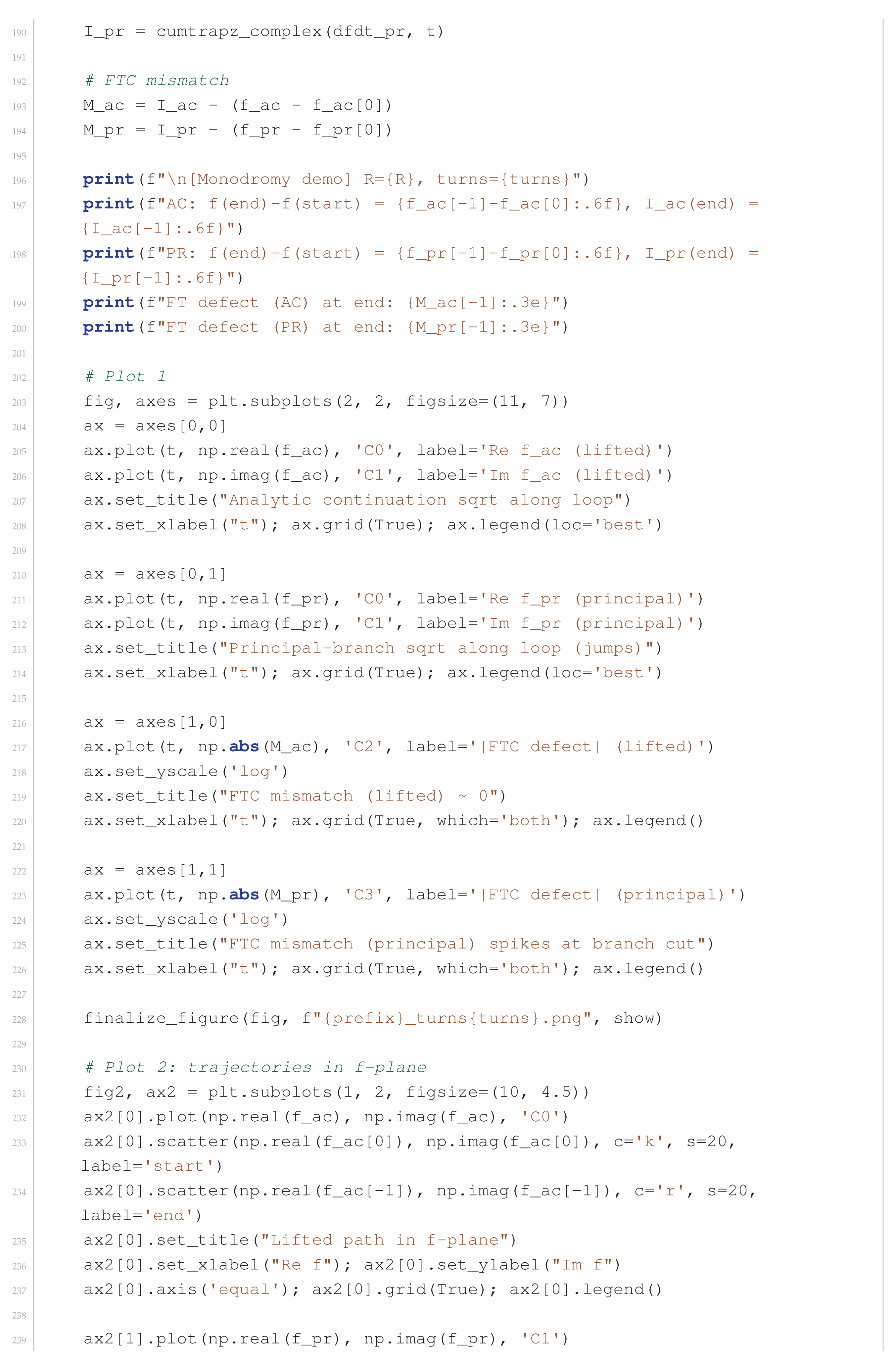
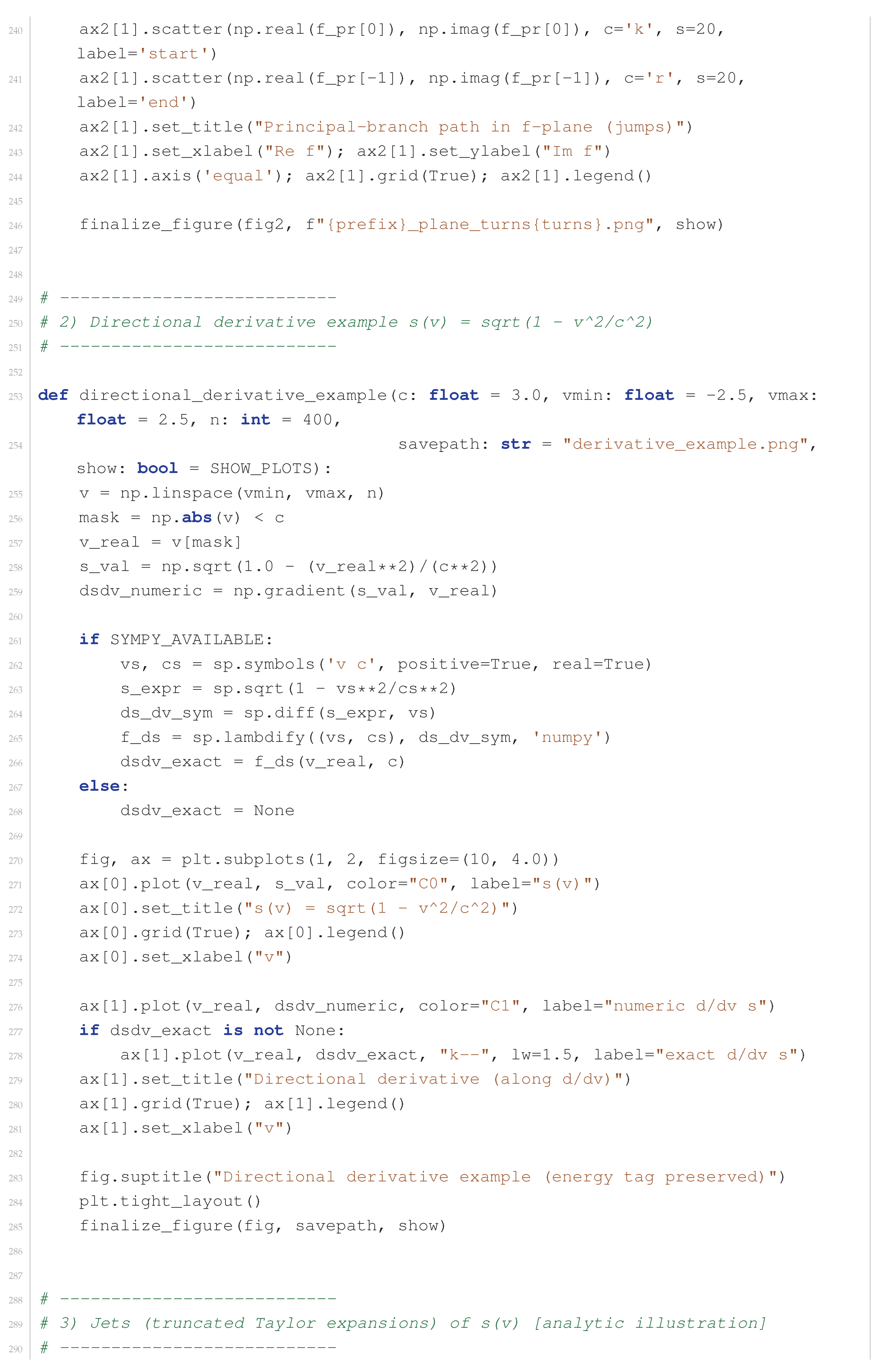
- monodromy-consistent differentiation along lifted paths (vs. principal-branch failure);
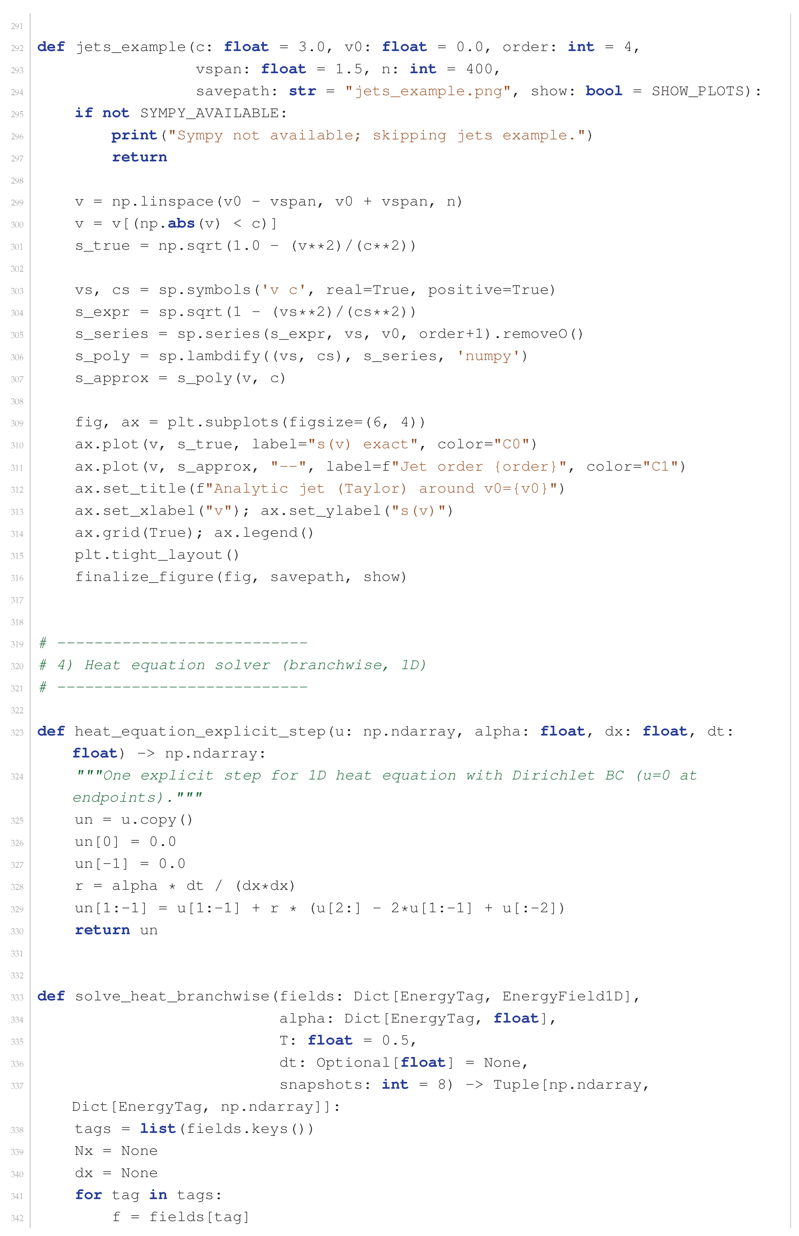
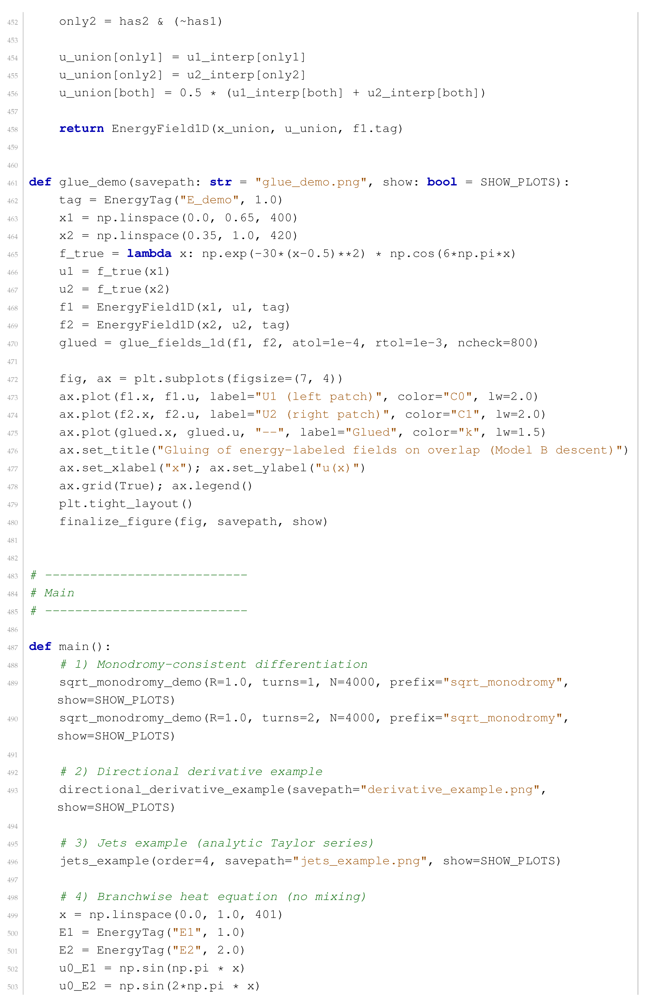
- numerical branchwise heat flow with no label mixing;
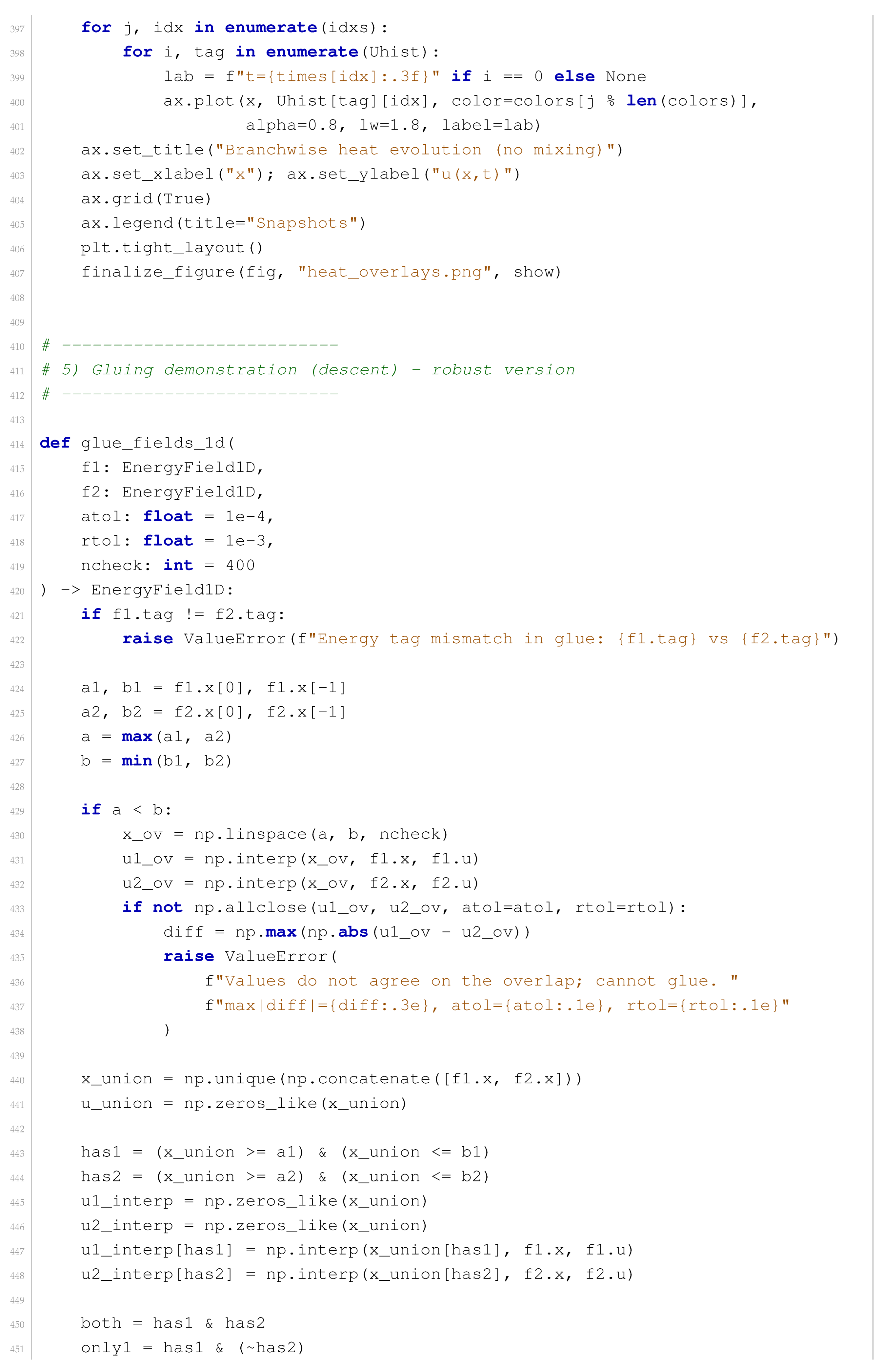
- a basic descent/gluing check enforcing label compatibility;
- (elliptic case) numerical Gauss–Manin transport for and and detection of logarithmic monodromy around .
- Dependencies. The first script uses numpy and matplotlib; it optionally uses sympy. The second script uses numpy, matplotlib, and mpmath.
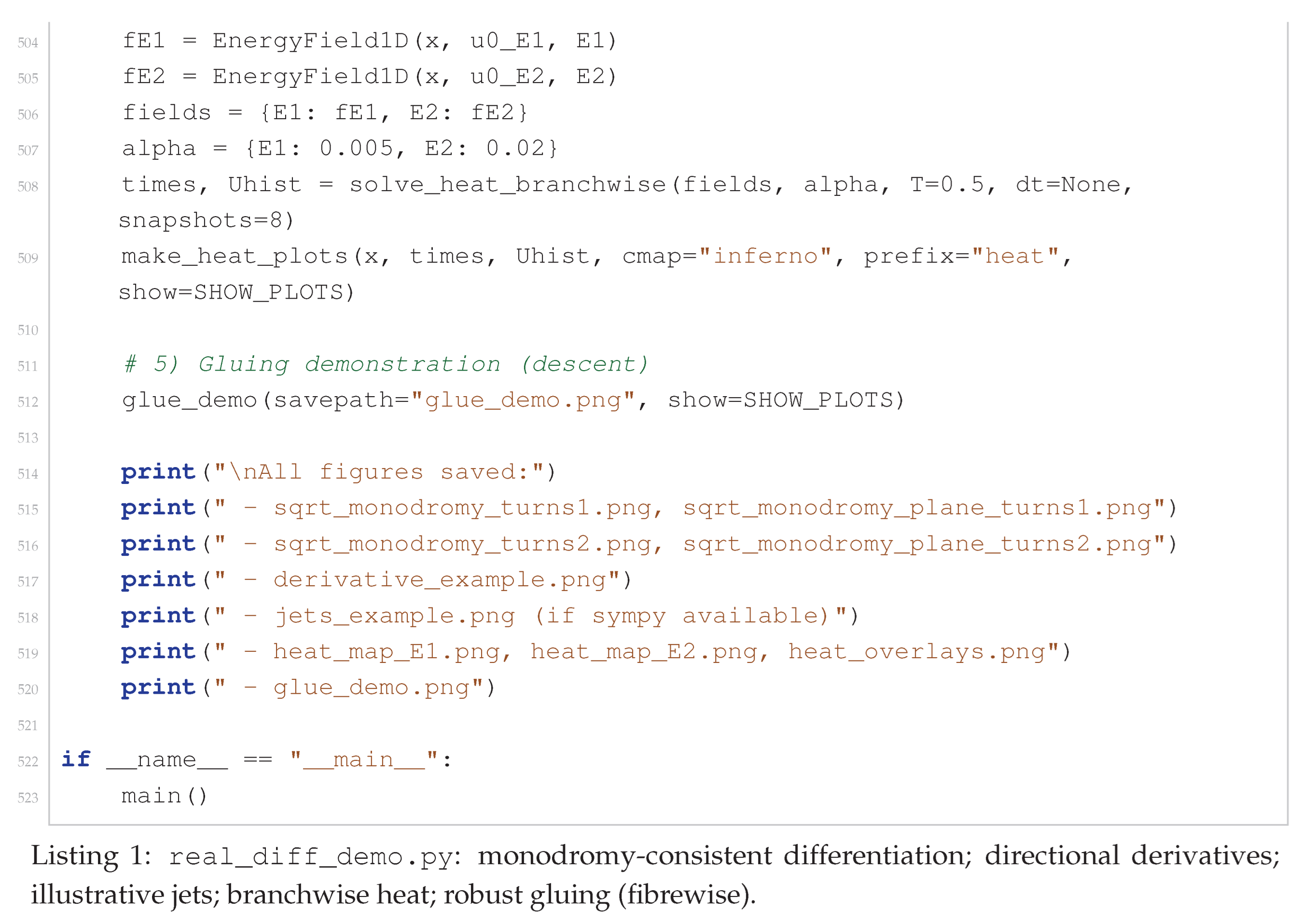
- Outputs. The scripts save figures to PNG files. The appendix figures below are representative outputs (filenames as provided).
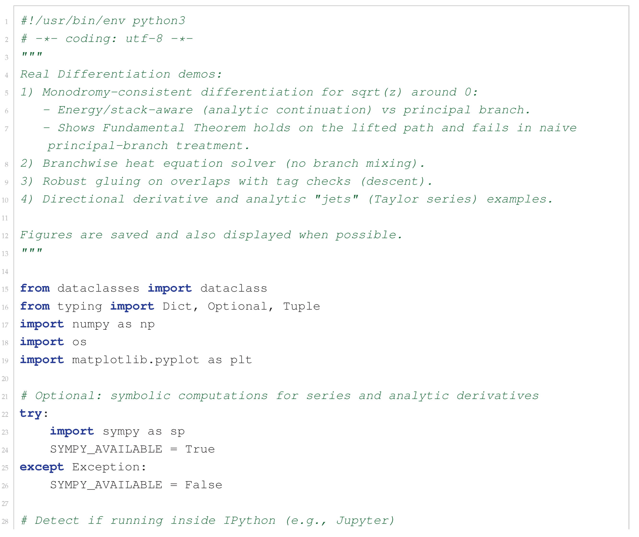
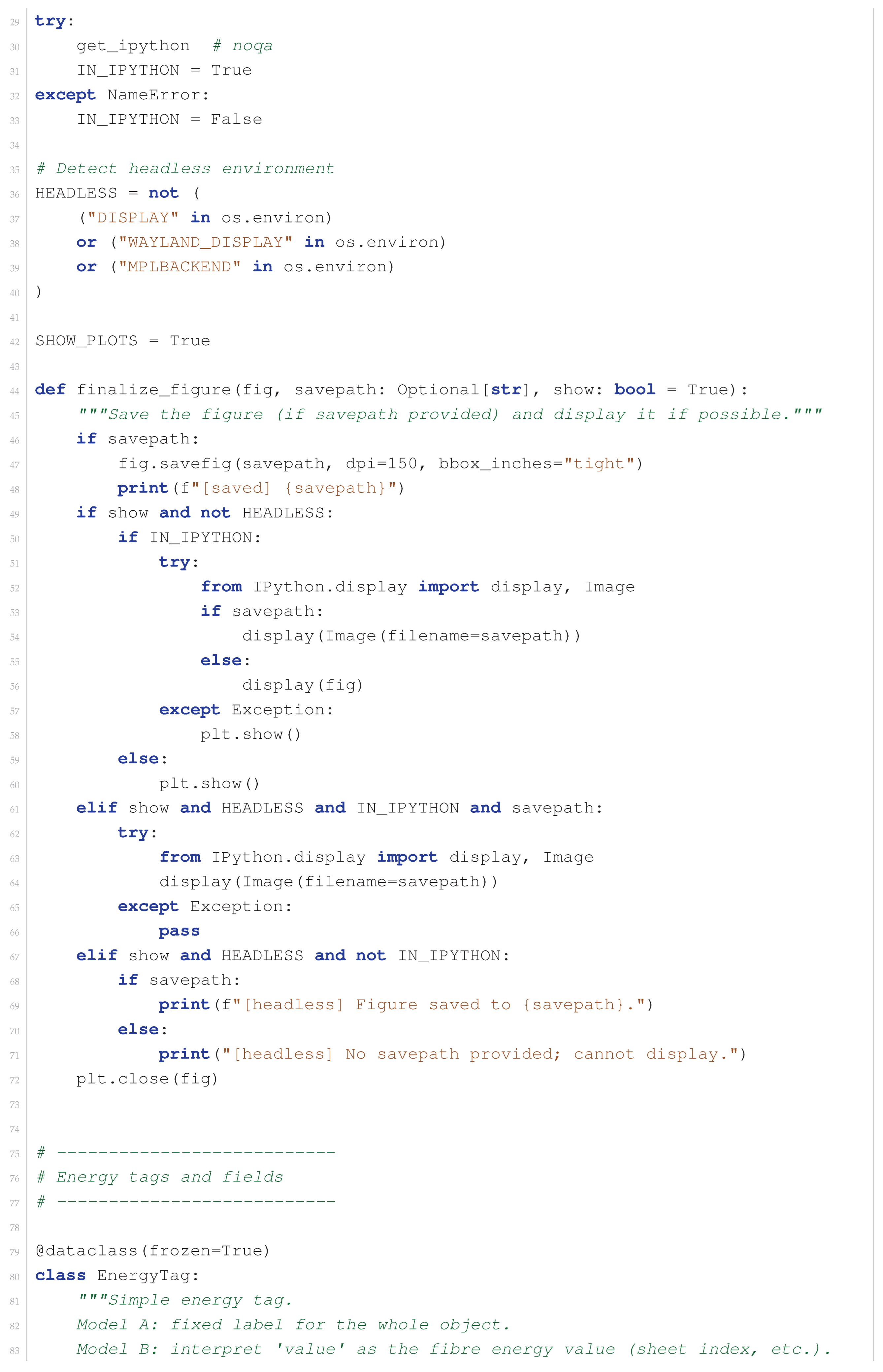
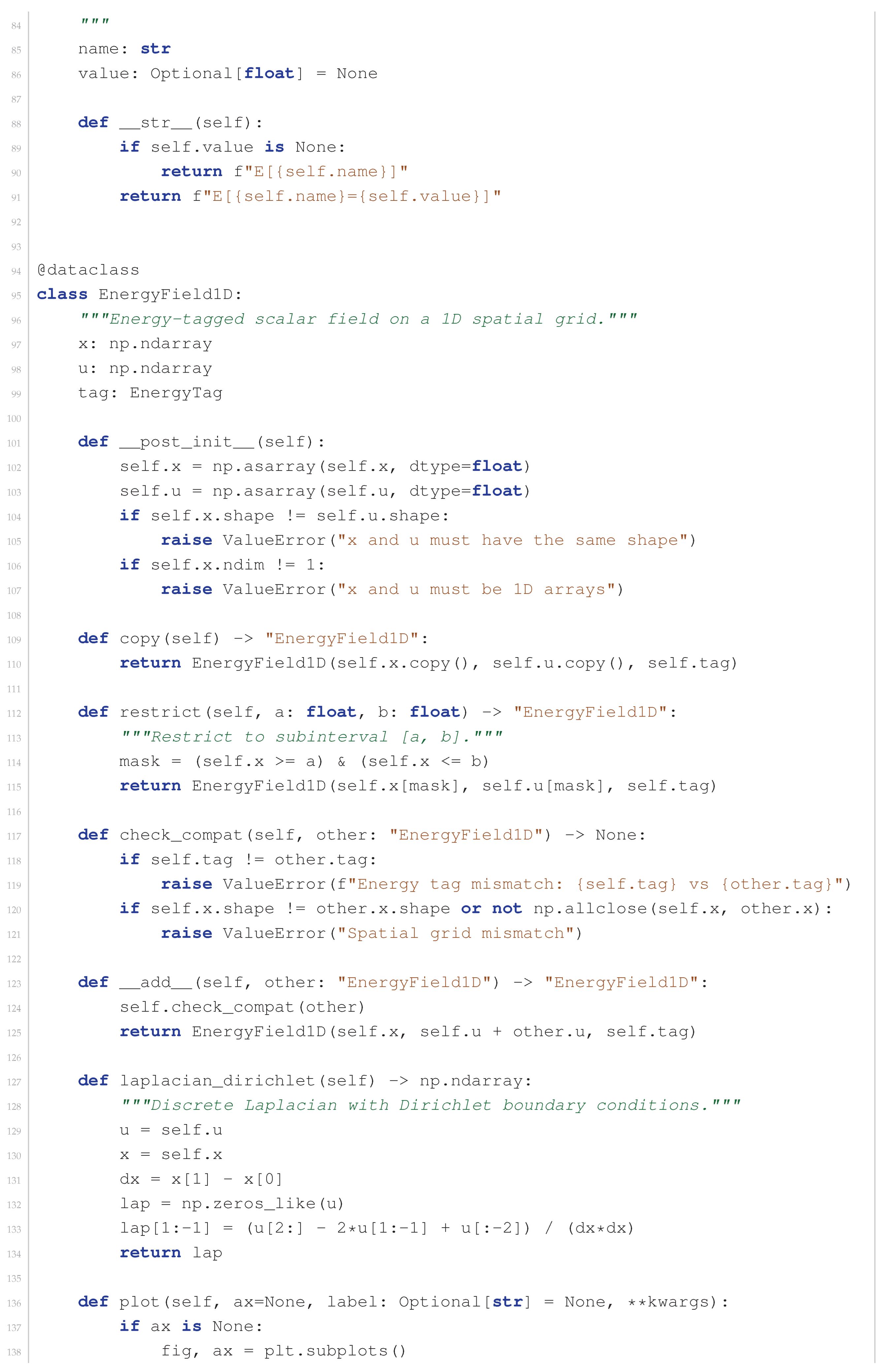
Appendix A.2. Listing: real_diff_demo.py
Appendix A.3. Listing: rd_elliptic_monodromy.py
Appendix B. Figures (Representative Outputs)
Remark A1.
For journal submission, we strongly recommend renaming files to stable descriptive names (e.g.sqrt_monodromy_turns1.png) and updating captions to match exact content. The figures below are included with the filenames provided.
Figure A1.
Representative computational output (1) from the accompanying scripts.
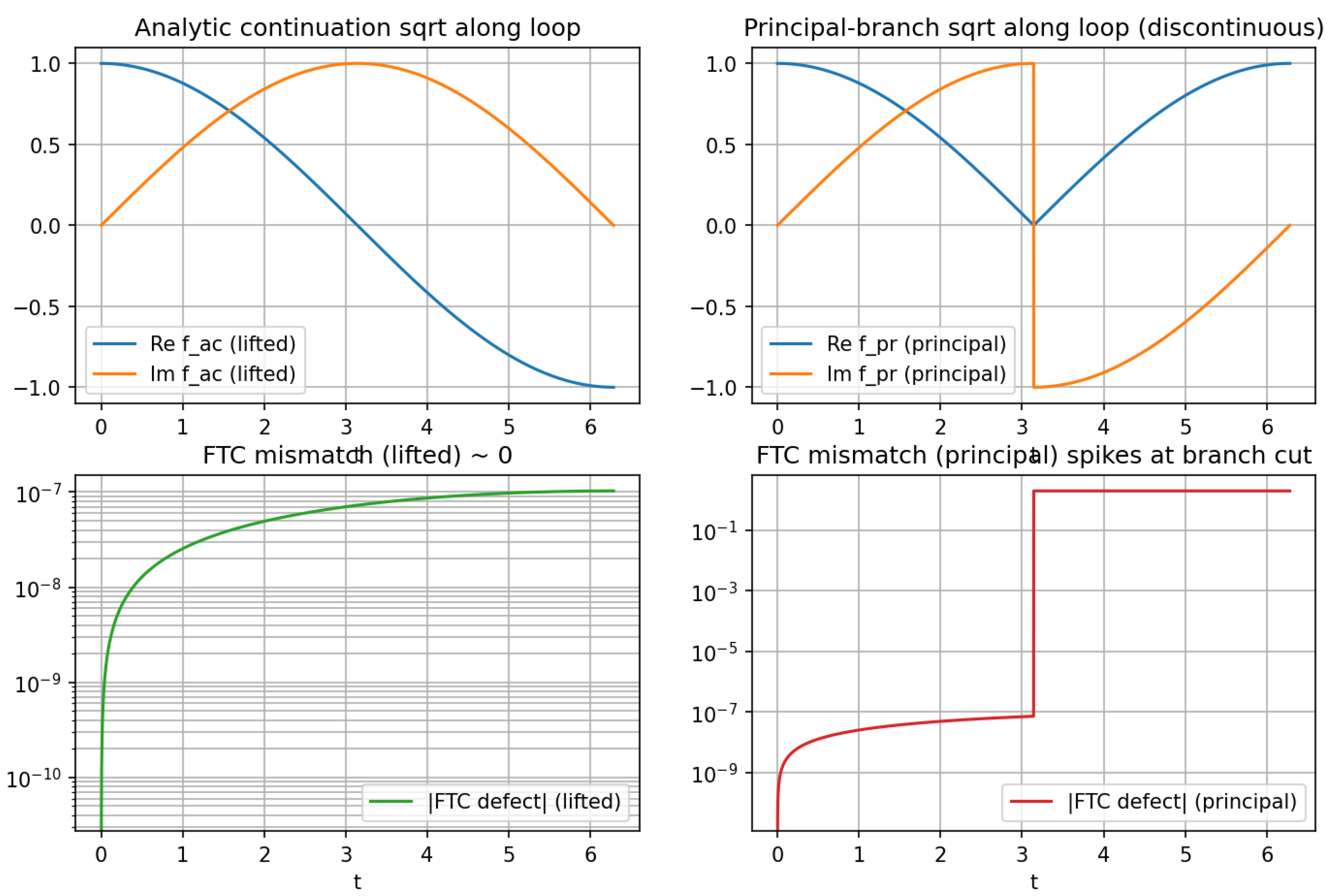
Figure A2.
Representative computational output (2) from the accompanying scripts.
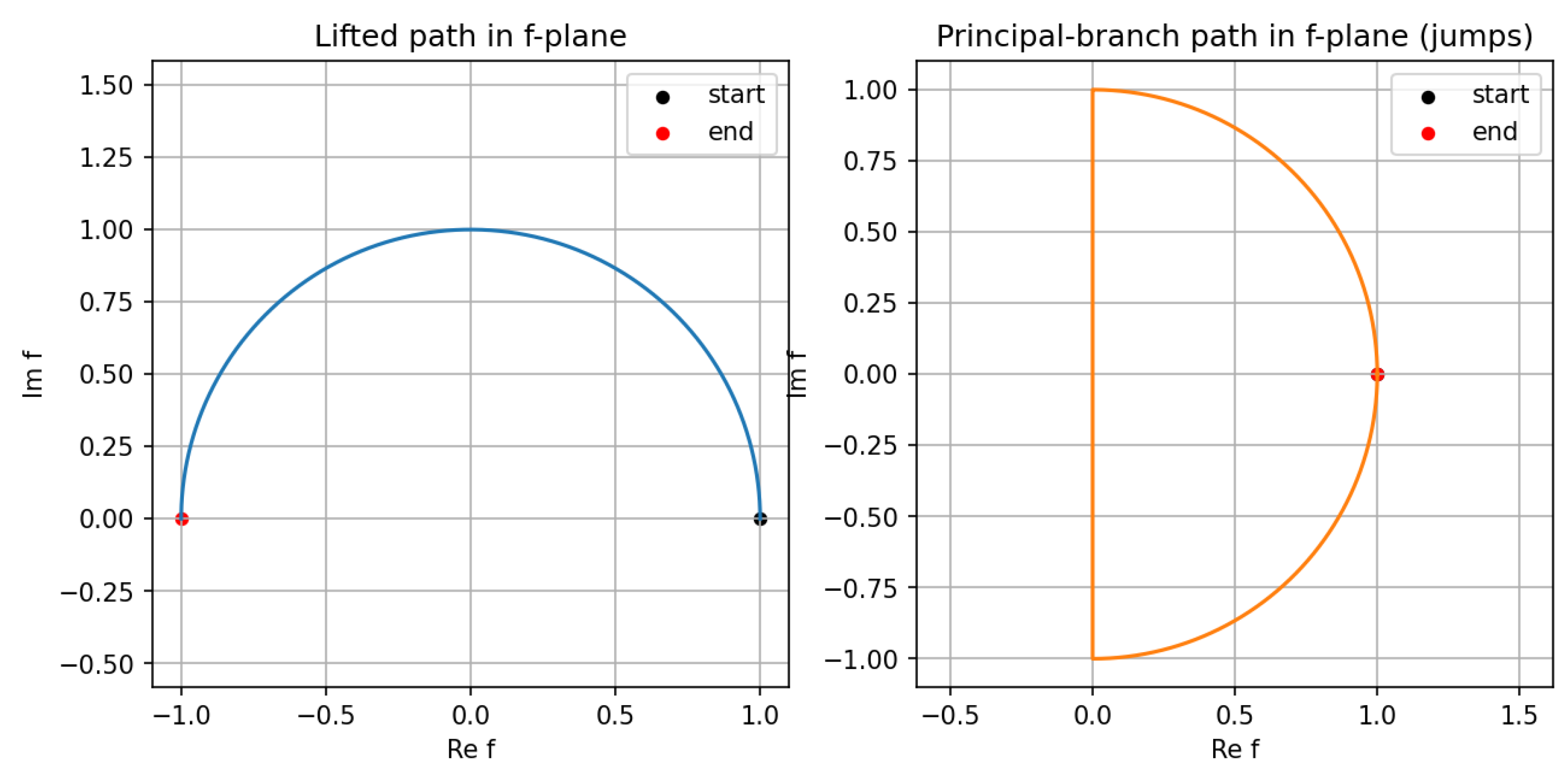
Figure A3.
Representative computational output (3) from the accompanying scripts.
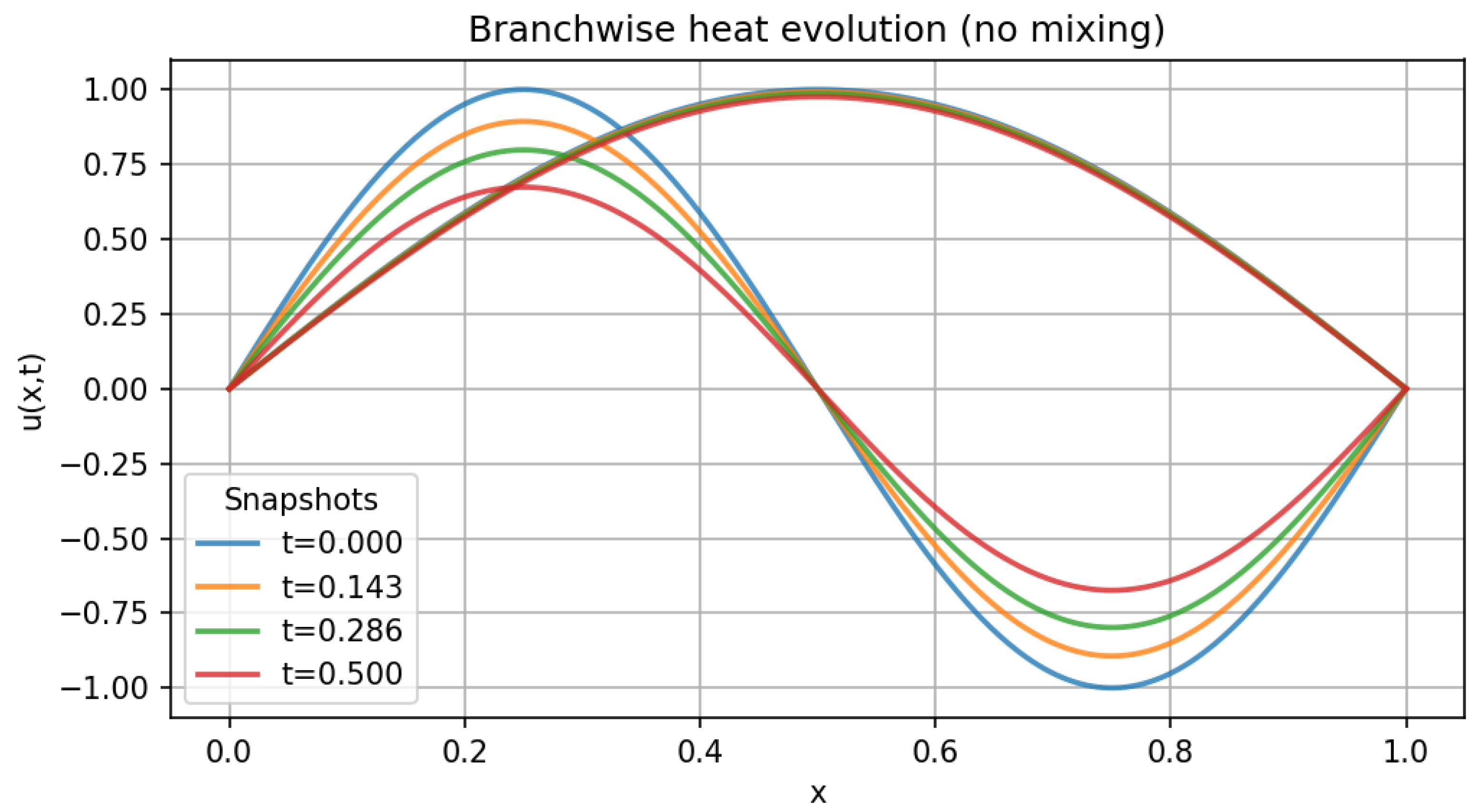
Figure A4.
Representative computational output (4) from the accompanying scripts.
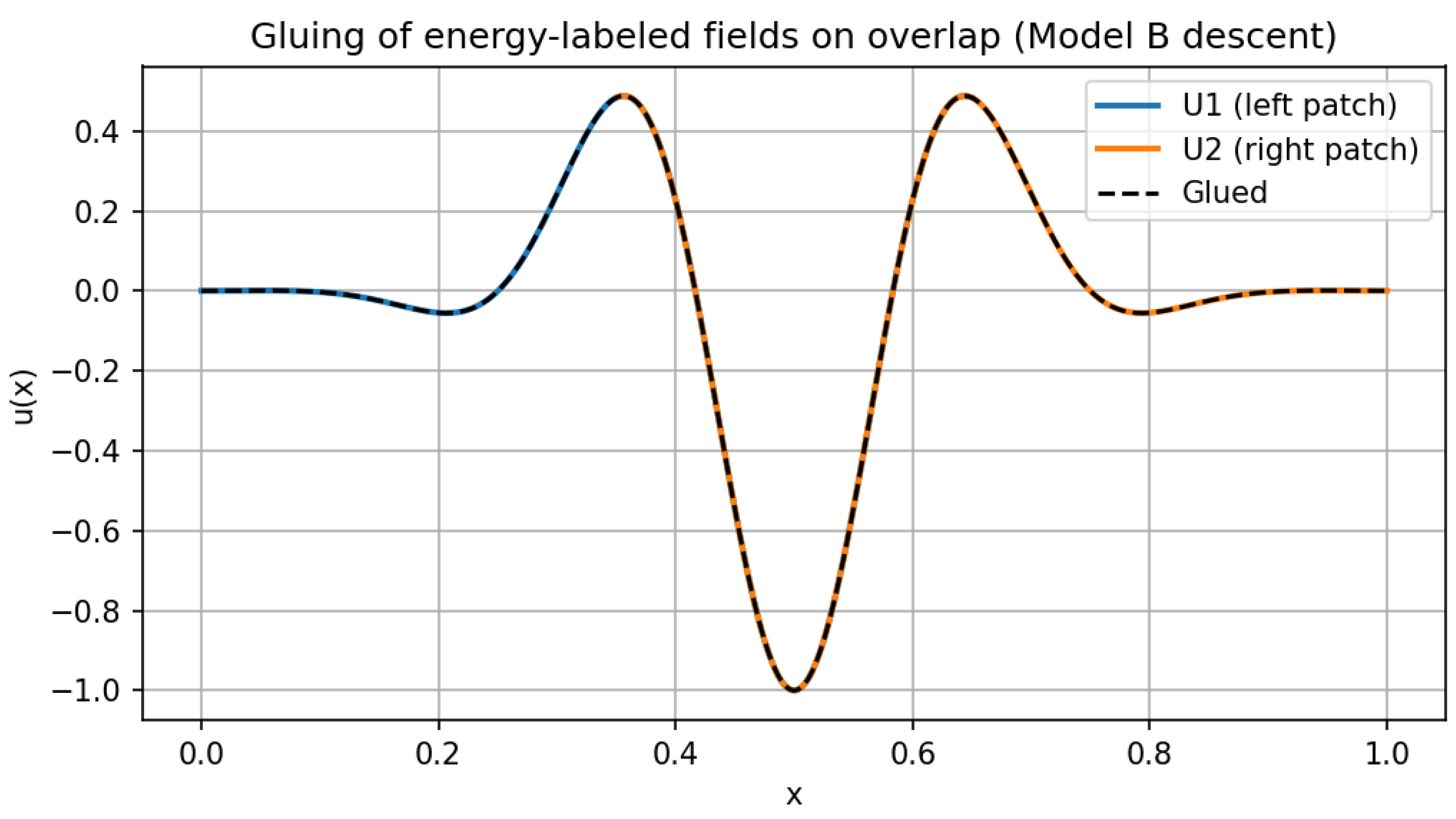
Figure A5.
Representative computational output (5) from the accompanying scripts.
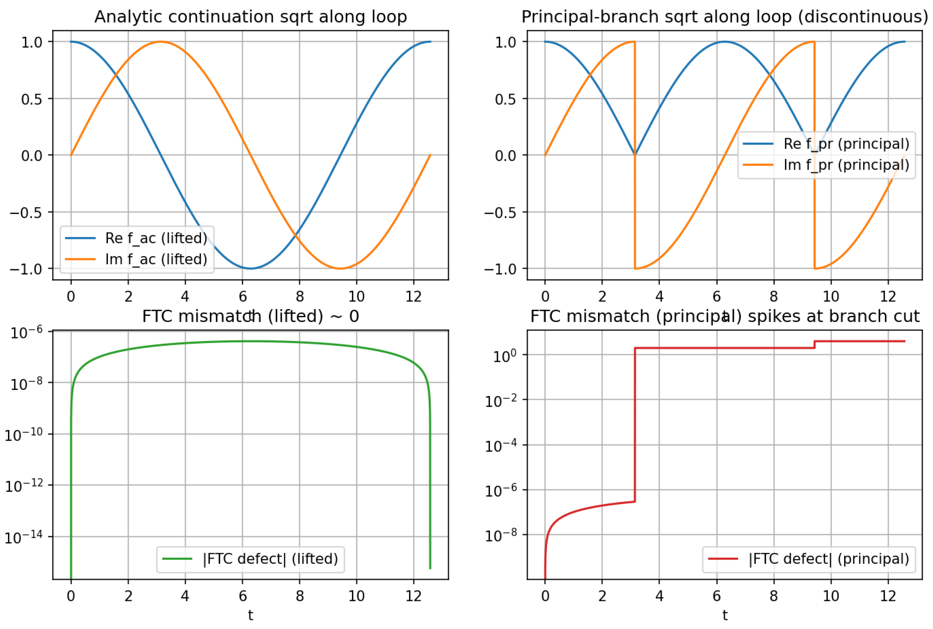
Figure A6.
Representative computational output (6) from the accompanying scripts.
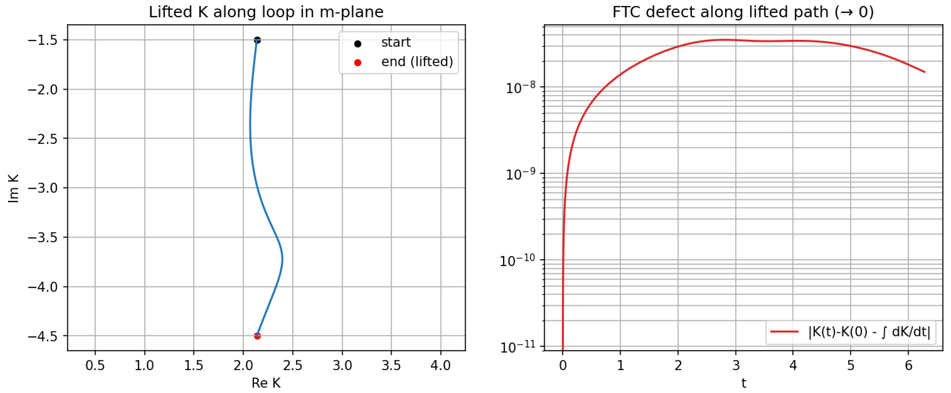
Figure A7.
Representative computational output (7) from the accompanying scripts.
References
- A. Grothendieck and J. Dieudonné. Éléments de Géométrie Algébrique IV. Publ. Math. IHÉS, 1964–1967.
- R. Hartshorne. Algebraic Geometry. Graduate Texts in Mathematics, Vol. 52. Springer, 1977.
- L. Illusie. Complexe Cotangent et Déformations I. Lecture Notes in Mathematics, Vol. 239. Springer, 1971.
Disclaimer/Publisher’s Note: The statements, opinions and data contained in all publications are solely those of the individual author(s) and contributor(s) and not of MDPI and/or the editor(s). MDPI and/or the editor(s) disclaim responsibility for any injury to people or property resulting from any ideas, methods, instructions or products referred to in the content. |
© 2025 by the authors. Licensee MDPI, Basel, Switzerland. This article is an open access article distributed under the terms and conditions of the Creative Commons Attribution (CC BY) license (http://creativecommons.org/licenses/by/4.0/).
Copyright: This open access article is published under a Creative Commons CC BY 4.0 license, which permit the free download, distribution, and reuse, provided that the author and preprint are cited in any reuse.


