A Convolutional Autoencoder-Based Method for Vector Curve Data Compression

1. Introduction

Vector spatial data constitute a fundamental component of geographic information systems (GIS), typically represented by point, line, and polygon features. From a geometric perspective, both line and polygon features can be expressed as ordered coordinate sequences, with polygons essentially forming closed curves. Together, line- and polygon-based data constitute a substantial proportion of spatial datasets and are often characterized by high vertex density and complex geometric structures. With the continuous growth of large-scale geographic databases, the storage, management, and transmission of vector line data have become increasingly challenging under constraints of limited storage capacity and network bandwidth. Therefore, efficient compression of vector curve data, while preserving essential geometric characteristics, has become a critical issue in geographic information science. Traditionally, the reduction of vector data volume has been closely associated with multi-scale cartographic representation. In map production, the same geographic feature must be represented at varying levels of detail depending on map scale, and geometric simplification is commonly applied when transitioning from large-scale to small-scale representations. The Douglas–Peucker (DP) algorithm is a classical approach that iteratively removes vertices whose perpendicular distance from the baseline connecting the start and end points falls below a predefined threshold, and it has been widely used due to its simplicity and effectiveness [1]. Numerous studies have further investigated and extended the DP algorithm. Yang et al. proposed a recursive implementation and introduced radial distance as a supplementary constraint to control area error while preserving curve smoothness [2]. They also pointed out that the lack of topological constraints in the classical DP algorithm may lead to self-intersections and that uncertainty in threshold selection can significantly affect simplification results. Subsequently, Li et al. refined the threshold search range and improved simplification performance by preserving key bends in polyline geometry [3]. Yu et al. enhanced DP-based simplification by selecting convex points of natural shorelines as candidate points and identifying segmentation points using angular and distance criteria, thereby improving both compression ratio and curve accuracy [4]. Beyond DP-based methods, other strategies have been proposed to achieve data reduction. Hybrid approaches combining genetic algorithms with local search strategies have been developed to balance shape preservation and compression efficiency [5]. However, the use of fixed coding lengths in such methods may result in increased storage and computational costs when applied to dense curves. Resampling-based techniques represent another class of methods, where curves are compressed by introducing new points located on or near the original geometry. The Li–Openshaw algorithm, for example, simulates human visual perception by retaining fine details at close observation distances while preserving only macroscopic shapes at smaller scales [6]. Function-fitting approaches provide a different perspective by representing line features with compact parametric forms. Fourier series–based methods [7,8,9,10] and wavelet-based fitting techniques [11,12] decompose curve geometry across multiple scales, preserving primary structural information while discarding secondary details.

Although these traditional methods are effective for scale-dependent representation, they are primarily designed for cartographic generalization, where data reduction serves visualization and map readability purposes. In such methods, compression ratios are usually determined indirectly by scale-related thresholds or perceptual criteria, rather than being explicitly optimized for storage efficiency. Moreover, most of these approaches are inherently lossy and irreversible, making it difficult to accurately reconstruct original geometric features from compressed representations. These limitations restrict their applicability in storage-oriented compression scenarios, where compact encoding and faithful geometric restoration are equally required for data archiving, transmission, and reuse in GIS databases. With the rapid development of deep learning, data-driven approaches have attracted increasing attention in spatial data processing and offer new possibilities for learning geometric representations directly from data. Neural network–based methods have been applied to polyline simplification and geometric feature extraction, demonstrating the feasibility of learning-based strategies for curve processing [13]. Convolutional neural networks have been employed to identify curve features after rasterization, generating candidate regions and removing redundant segments [14]. Other studies have explored supervised and unsupervised learning frameworks for vector data compression and reconstruction. Encoder–decoder architectures have been used for rasterized road integration [15], while generative adversarial networks have been applied to reconstruct simplified vector roads from raster images [16]. Autoencoder-based models have further been investigated for multi-level curve simplification and vertex pooling, enabling effective simplification of polylines and building outlines [17,18]. More recently, fully connected autoencoders have been applied to curve data compression and reconstruction, confirming the capability of neural networks to capture morphological features for efficient data reduction [19].

However, most existing learning-based approaches inherit the objectives of cartographic generalization, focusing on visual simplification or scale adaptation rather than explicit storage-oriented compression of vector curves. The learned latent representations are often not optimized for compact encoding, and reconstruction accuracy is typically evaluated under scale-dependent or qualitative criteria. Consequently, there remains a lack of learning-based methods specifically designed to achieve high-efficiency compression and reliable geometric reconstruction for vector curve data in GIS storage and transmission contexts.

To address this limitation, this study proposes a convolutional autoencoder-based compression framework for vector curve data. The proposed method operates directly on vector curve representations, employing curve segmentation and resampling to standardize input data. By integrating convolutional neural networks and fully connected layers, the model jointly captures local geometric structures and global shape characteristics, enabling compact latent encoding and accurate curve reconstruction. Island boundary data are adopted as representative free-form vector curves with complex geometry and multi-scale characteristics. Owing to its generic formulation, the proposed framework can be extended to other types of vector line data. Experimental results demonstrate that the proposed method achieves improved compression efficiency while maintaining high reconstruction accuracy, making it suitable for storage-oriented compression of vector curves in GIS applications. It should be emphasized that the proposed method targets storage-oriented vector data compression rather than cartographic generalization, with the primary objective of achieving compact representation and accurate reconstruction of original geometries.

2. Model and Methods

To achieve storage-oriented compression of vector curve data while preserving geometric fidelity, this study formulates vector curve compression as a representation learning problem rather than a scale-driven simplification task. The core objective is to encode vector curves into compact latent representations that enable efficient storage and transmission, while allowing accurate reconstruction of the original geometry under controlled distortion. Unlike traditional cartographic generalization methods, where data reduction is implicitly determined by scale-dependent thresholds, the proposed approach explicitly optimizes the balance between compression efficiency and reconstruction accuracy through a data-driven encoding–decoding framework. Vector curves are treated as ordered sequences of coordinates, and their geometric characteristics are captured through standardized segmentation and resampling to ensure consistent input representation. To effectively model both local geometric variations and global curve structures, a convolutional autoencoder architecture is adopted. Convolutional layers are employed to learn local geometric patterns and continuity along the curve, while fully connected layers capture global shape information and perform compact latent encoding. This integrated design enables the proposed method to learn efficient representations directly from vector data without rasterization, making it particularly suitable for storage-oriented compression of complex geographic curves.

2.1. Problem Formulation and Curve Representation

Vector curve data in GIS are typically represented as ordered sequences of two-dimensional coordinates that describe the geometric shape of linear or boundary features. Given a vector curve C=$\{\left({\mathrm{x}}_1,{\mathrm{y}}_1\right),\left({\mathrm{x}}_2,{\mathrm{y}}_2\right)\dots ,({\mathrm{x}}_{\mathrm{n}},{\mathrm{y}}_{\mathrm{n}}\left)\right\}$, where the points are ordered along the curve, the objective of vector curve compression is to reduce the amount of data required to store and transmit C while preserving its essential geometric characteristics. In storage-oriented compression scenarios, the goal differs fundamentally from scale-driven cartographic generalization. Rather than selectively removing vertices based on perceptual or scale-dependent thresholds, storage-oriented compression seeks to encode the original curve into a compact representation z such that the reconstructed curve $\overline{\mathrm{C}}$ can be faithfully recovered from z under controlled geometric distortion. This process can be formulated as an encoding–decoding problem, where an encoder function $\mathrm{f}(\cdot )$ maps the original curve C to a latent representation z=$\mathrm{f}\left(\mathrm{C}\right)$, and a decoder function $\mathrm{g}(\cdot )$ reconstructs the curve as $\overline{\mathrm{C}}=\mathrm{g}\left(z\right)$.

A key challenge in learning-based vector curve compression lies in the variable length and non-uniform sampling of vector curves. Geographic curves often exhibit irregular vertex spacing and highly variable geometric complexity, which makes it difficult to directly apply neural network models that require fixed-length inputs. To address this issue, the proposed framework adopts a standardized curve representation through segmentation and resampling, transforming curves of arbitrary length into consistent representations while preserving their geometric continuity. This enables the learning of compact encodings across curves with diverse shapes and lengths.

To enhance the modeling of geometric structure, vector curves are represented using coordinate differences rather than absolute coordinates. Specifically, the curve is expressed as a sequence of incremental displacements between consecutive vertices, which emphasizes local geometric variation and reduces sensitivity to absolute position. This representation facilitates the learning of translation-invariant geometric patterns and supports efficient reconstruction by cumulatively restoring vertex positions from the decoded displacement sequence. Based on this formulation, vector curve compression is treated as a representation learning problem in which the encoder learns a compact latent representation that captures both local geometric details and global curve structure. The reconstruction quality is evaluated by comparing the original curve C and the reconstructed curve $\overline{\mathrm{C}}$ using geometric error measures defined in Section 2.4. This formulation provides a unified foundation for the convolutional autoencoder-based compression framework described in the following sections.

2.2. Data Preprocessing

Spatial vector line data are commonly represented as ordered sequences of Cartesian coordinates, expressed as $\{\left({\mathrm{x}}_1,{\mathrm{y}}_1\right),\left({\mathrm{x}}_2,{\mathrm{y}}_2\right)\dots \dots \}$, where each point records its spatial location along the curve. While absolute coordinates describe positional information, the geometric characteristics of a curve—such as direction changes and local shape variations—are more effectively captured by the differences between adjacent points. Therefore, the present study represents curve geometry using coordinate increments, i.e., incremental changes in Cartesian coordinates between consecutive vertices. Specifically, for each curve segment, the coordinate differences $\left(\mathrm{d}{\mathrm{x}}_{\mathrm{i}},\mathrm{d}{\mathrm{y}}_{\mathrm{i}}\right)$ are computed between adjacent points. By recording the absolute coordinates of the first point and cumulatively summing the coordinate increments, the original curve geometry can be fully reconstructed. This representation emphasizes local geometric variation while reducing sensitivity to absolute position, making it well suited for learning-based compression. Based on this principle, coordinate increments are employed as feature vectors and input into the convolutional autoencoder model for training. Neural network models typically require inputs of fixed length and consistent structure. However, island boundary data exhibit substantial variability in curve length, shape complexity, and point distribution. To address these challenges and ensure data consistency, a preprocessing pipeline consisting of curve segmentation, curve resampling, and data normalization is applied, as described below.

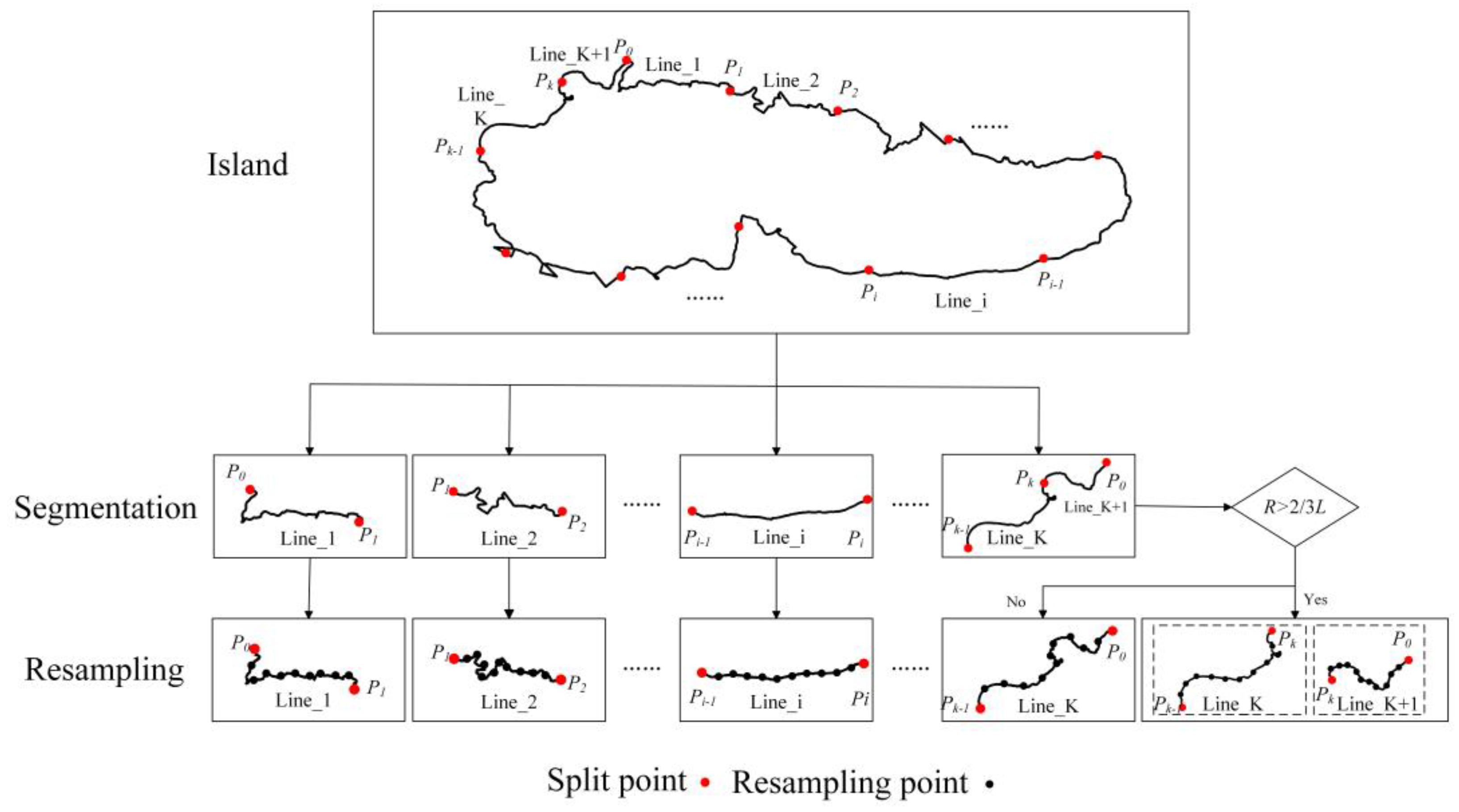
2.2.1. Curve Segmentation

Island boundary curves vary significantly in total length, and excessive variation in segment length can introduce large discrepancies in geometric complexity, thereby increasing the difficulty of neural network training. To reduce this effect, each boundary curve with total length $\mathrm{L}$ is divided into multiple sub-segments with a target length $\mathrm{l}$. In general, if$\mathrm{L}>\mathrm{l}$, the curve is initially divided into $\mathrm{k}>[\mathrm{L}/\mathrm{l}]$. sub-segments of length $\mathrm{l}$, leaving a remaining portion of length $\mathrm{e}=\mathrm{L}-\mathrm{k}\mathrm{*}\mathrm{l}$. Since the final sub-segment may not meet the target length, two cases are considered to handle the remainder:

1. If $\mathrm{e}<{\displaystyle \frac{2}{3}}l$, the remaining portion is sufficiently short and is merged with the k-th segment. In this case, the adjusted length of the k-th segment becomes ${\mathrm{l}}_{\mathrm{k}}=\mathrm{L}-\left(\mathrm{k}-1\right)\mathrm{*}\mathrm{l}$.

2. If $\mathrm{e}\ge {\displaystyle \frac{2}{3}}\mathrm{l}$, the remaining portion is retained as an additional segment, denoted as the $(\mathrm{k}+1)$-th segment, with length ${\mathrm{l}}_{\mathrm{k}+1}=\mathrm{e}$.

This segmentation strategy ensures that segment lengths remain relatively consistent while avoiding excessively short segments, thereby preserving the geometric characteristics of the original boundary curve.

2.2.2. Curve Resampling

After segmentation, individual curve segments may still differ in the number of vertices they contain. Since neural networks require inputs of uniform size, resampling is applied to standardize point distributions across segments. In addition, uneven vertex spacing within a segment can adversely affect model training. To address these issues, equidistant resampling is employed. For a curve segment with length${\mathrm{l}}_{\mathrm{i}}$, the segment is resampled into $\mathrm{N}$ equal intervals with a sampling distance of ${\mathrm{l}}_{\mathrm{i}}/\mathrm{N}$, producing $\mathrm{N}+1$ uniformly distributed points. The coordinate differences between consecutive resampled points are then computed, resulting in a sequence of $\mathrm{N}$ incremental vectors ${(\mathrm{d}\mathrm{x}}_{\mathrm{i}},{\mathrm{d}\mathrm{y}}_{\mathrm{i}})$, where $\mathrm{i}=\mathrm{1,2},\dots ,\mathrm{N}$. This procedure yields a fixed-length representation for each curve segment while maintaining its overall geometric structure. The segmentation and resampling process is illustrated in Figure 1.

2.2.3. Data Normalization

To improve the efficiency and stability of neural network training, the coordinate increment features are normalized prior to model input. Specifically, the coordinate differences are scaled to the range [0,1] using min–max normalization, as expressed in Equation (1):

$$\left.\begin{array}{c}△{\mathrm{x}}_{\mathrm{i}}={\displaystyle \frac{\mathrm{d}{\mathrm{x}}_{\mathrm{i}}-{\mathrm{d}\mathrm{x}}_{\mathrm{m}\mathrm{i}\mathrm{n}}}{{\mathrm{d}\mathrm{x}}_{\mathrm{m}\mathrm{a}\mathrm{x}}-{\mathrm{d}\mathrm{x}}_{\mathrm{m}\mathrm{i}\mathrm{n}}}}\\ △{\mathrm{y}}_{\mathrm{i}}={\displaystyle \frac{\mathrm{d}{\mathrm{y}}_{\mathrm{i}}-{\mathrm{d}\mathrm{y}}_{\mathrm{m}\mathrm{i}\mathrm{n}}}{{\mathrm{d}\mathrm{y}}_{\mathrm{m}\mathrm{a}\mathrm{x}}-{\mathrm{d}\mathrm{y}}_{\mathrm{m}\mathrm{i}\mathrm{n}}}}\end{array}\right\}$$

(1)

Where ${\mathrm{d}\mathrm{x}}_{\mathrm{m}\mathrm{i}\mathrm{n}}$​ and ${\mathrm{d}\mathrm{x}}_{\mathrm{m}\mathrm{a}\mathrm{x}}$ denote the minimum and maximum values of the x-coordinate increments within a segment, and ${\mathrm{d}\mathrm{y}}_{\mathrm{m}\mathrm{i}\mathrm{n}}$​ and ${\mathrm{d}\mathrm{x}}_{\mathrm{m}\mathrm{a}\mathrm{x}}$ denote the corresponding values for the y-coordinate increments. Normalization ensures consistent feature scaling and prevents variables with larger magnitudes from dominating the training process.

2.3. Convolutional Autoencoder-based Compression Model

2.3.1. Convolutional Autoencoder

Convolutional neural networks (CNNs) were first introduced to process data with local spatial correlations and have since been widely applied in raster image processing [20]. CNNs are capable of automatically learning hierarchical and discriminative feature representations, ranging from low-level to high-level features. They are capable of automatically learning hierarchical and discriminative feature representations, ranging from low-level to high-level features. The key parameters of the convolution operation are convolution kernels, which are trainable weights within the network. Compared to fully connected layers, CNNs typically require significantly fewer parameters. The general computational model of a CNN is expressed in Equation (2):

$$\mathrm{y}=\mathrm{h}\left(\mathrm{X}⨂\mathrm{W}+\mathrm{b}\right)$$

(2)

where $\mathrm{X}$ denotes the input, $\mathrm{W}$ denotes the convolution kernel, $\mathrm{b}$ denotes the bias, $\mathrm{h}(\cdot )$ denotes the activation function, and $\mathrm{y}$ the output. The symbol $⨂$ denotes the convolution operation.

In practice, convolution performs a feature extraction process that can be viewed as a form of downsampling. Repeated convolutions progressively filter and abstract the input, enabling the extraction of salient information from complex data. To reconstruct data, a transposed convolution (also known as deconvolution) is used. Unlike standard convolution, which relies on fixed operations, transposed convolution employs learnable parameters that allow the network to automatically learn an appropriate upsampling strategy, thereby supporting data reconstruction.

Autoencoders provide an unsupervised learning framework for dimensionality reduction and data reconstruction and have been extensively used in representation learning [21]. They consist of two components: an encoder, which compresses high-dimensional input ($\mathrm{d}\mathrm{x},\mathrm{d}\mathrm{y})$ into a low-dimensional representation z, and a decoder, which maps z back to an output ($\mathrm{d}\overline{\mathrm{x}},\mathrm{d}\overline{\mathrm{y}})$ of the same dimensionality as ($\mathrm{d}\mathrm{x},\mathrm{d}\mathrm{y})$. By minimizing the reconstruction error between X and Y, autoencoders learn compact latent representations of the data.

A convolutional autoencoder extends this principle by employing convolutional layers as its encoder and transposed convolutional layers as its decoder. The encoder captures essential structural information by applying convolutions to coordinate difference sequences, thereby compressing the data into low-dimensional feature vectors. The decoder, with a symmetric architecture, applies transposed convolutions to reconstruct the coordinate differences, ultimately restoring the original data. Compared to fully connected autoencoders, convolutional autoencoders require fewer parameters while better preserving local spatial structures. Thus, if the discrepancy between ($\mathrm{d}\overline{\mathrm{x}},\mathrm{d}\overline{\mathrm{y}})$ and ($\mathrm{d}\mathrm{x},\mathrm{d}\mathrm{y})$ remains within an acceptable threshold, the low-dimensional latent vector z can be considered a valid representation of ($\mathrm{d}\mathrm{x},\mathrm{d}\mathrm{y})$, with z serving as its compressed form.

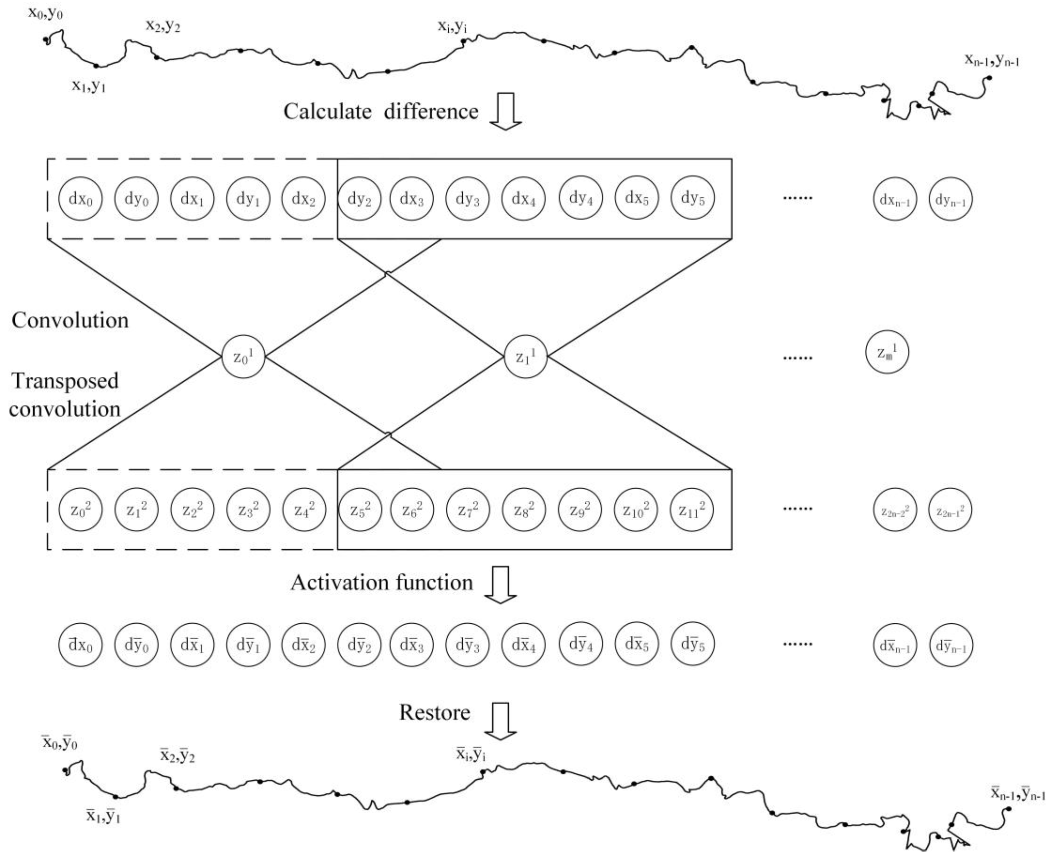
The architecture of the proposed convolutional autoencoder is illustrated in Figure 2. First, coordinate differences ($\mathrm{d}\mathrm{x},\mathrm{d}\mathrm{y})$ are computed to form the input sequence. A one-dimensional convolutional layer extracts features and reduces dimensionality, yielding a latent vector z₁. This compressed representation is then upsampled through transposed convolution to produce z₂. A nonlinear activation function transforms z₂ into the reconstructed output vector ($\mathrm{d}\overline{\mathrm{x}},\mathrm{d}\overline{\mathrm{y}})$, which has the same dimensionality as the input. Finally, the original coordinates are restored from the reconstructed differences.

2.3.2. Data Compression with a Convolutional Autoencoder

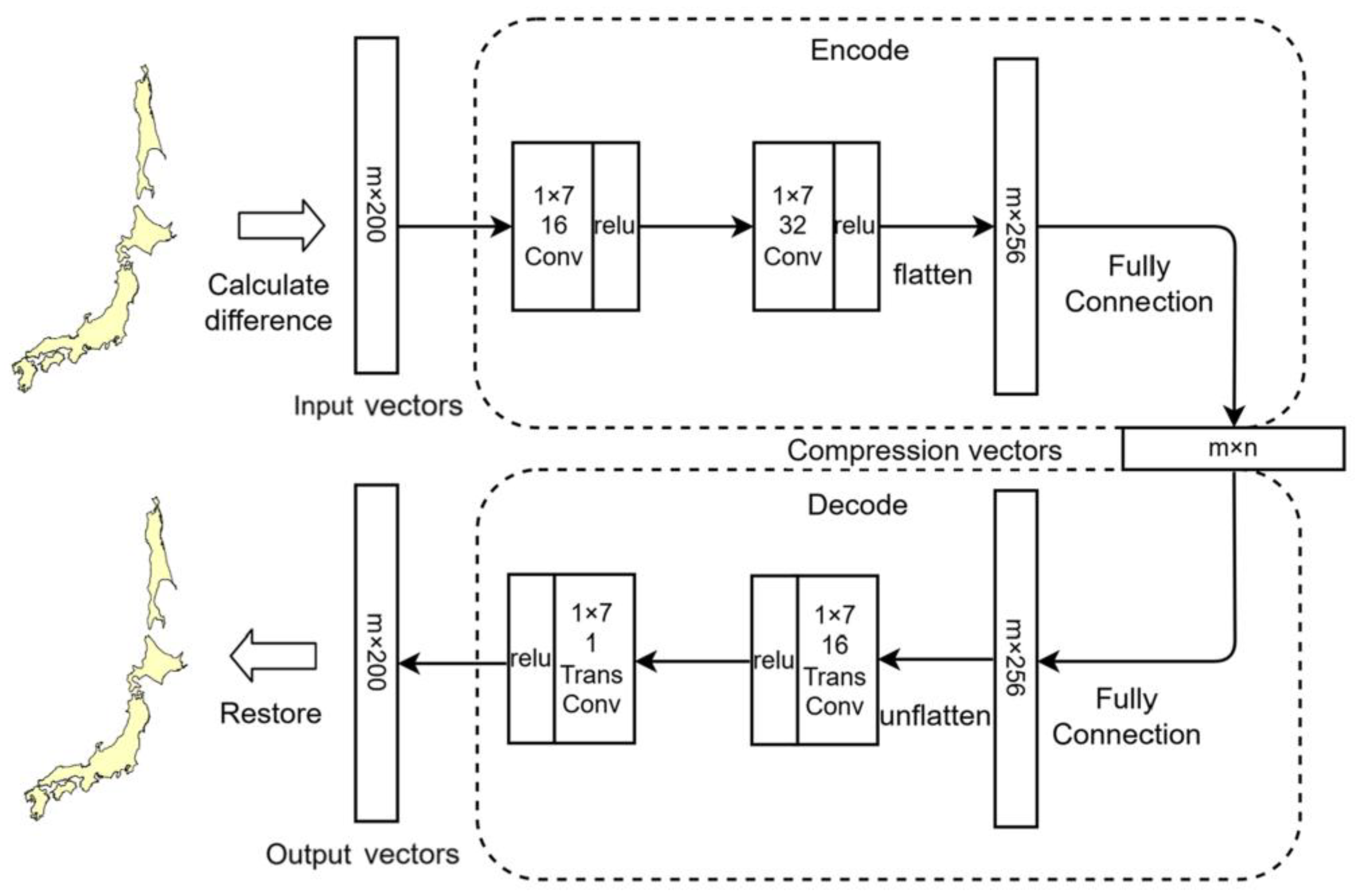
Convolutional neural networks (CNNs) are particularly effective in capturing local structural patterns while maintaining parameter efficiency, making them well suited for modeling sequential geometric data. Depending on the dimensionality of the input, convolutional operations can be implemented in different forms. In the present study, the training samples consist of ordered sequences of coordinate increments derived from segmented and resampled curves, which naturally correspond to one-dimensional signals. Accordingly, a one-dimensional convolutional autoencoder (CAE) is adopted to perform vector curve compression. A key challenge in CAE-based compression lies in controlling the dimensionality of the latent representation using convolutional layers alone. To explicitly regulate the compression ratio, a fully connected layer is introduced after the final convolutional layer in the encoder to map high-dimensional feature maps into a compact latent vector. To maintain architectural symmetry, a corresponding fully connected layer is placed at the beginning of the decoder. The overall architecture of the proposed model is illustrated in Figure 3. The encoder consists of two one-dimensional convolutional layers followed by a fully connected layer, whereas the decoder mirrors this structure using a fully connected layer and two transposed convolutional layers. The encoder outputs a low-dimensional latent vector that serves as the compressed representation of the curve segment, while the decoder reconstructs the coordinate increment sequence from this latent encoding. Since the input features are normalized to the range [0,1], the Rectified Linear Unit (ReLU) activation function is employed in all hidden layers. Reconstruction accuracy is measured using the root mean square error (RMSE), which is adopted as the loss function during training. The proposed CAE operates on generic curve representations derived from coordinate sequences and does not depend on semantic attributes of specific geographic objects, making it applicable to a wide range of vector line data.

To ensure sufficient overlap between convolutional receptive fields while preserving feature continuity, the stride of both convolutional and transposed convolutional layers is set to half of the kernel size. Empirical experiments demonstrate that a convolution kernel size of 1×7 yields optimal performance (Section 5.1), while a segment length of 25 km provides the best trade-off between geometric consistency and compression efficiency (Section 5.2). The first convolutional layer contains 16 channels and the second 32 channels, with the decoder adopting a symmetric configuration. The input feature vector has a fixed length of 200, which is compressed into a latent vector of dimension n, where n can be adjusted to achieve different compression ratios.

After training, the compressed representation of a curve dataset consists of three components: (1) the latent vectors produced by the encoder, (2) the starting coordinates of each curve segment, and (3) the trained model parameters (weights and biases). The model parameters are shared across all curve segments and are therefore stored only once. Although they formally belong to the compressed dataset, their contribution to the overall storage cost becomes negligible when the number of segments is sufficiently large. In practical experiments, the model size ranges from several tens to a few hundreds of kilobytes, which is minor compared with the size of the original vector data. The compression ratio is defined as the ratio between the size of the compressed data and that of the original curve data, as shown in Equation (3):

$$\mathrm{B}={\displaystyle \frac{\mathrm{M}\mathrm{*}(\mathrm{N}+1)+\mathrm{W}}{\mathrm{K}\mathrm{*}2\mathrm{P}}}\approx {\displaystyle \frac{\mathrm{N}}{2\mathrm{P}}}$$

(3)

where B denotes the compression ratio, M is the number of curve segments, P is the average number of sampled points per segment, N is the dimensionality of the latent vector, and W represents the total number of model parameters. When M is sufficiently large, the influence of W can be ignored, leading to the simplified expression shown in the second part of Equation (3).

2.3.3. Restoration of Island Boundary Data

Curve reconstruction begins by reversing the normalization applied during preprocessing, thereby restoring the coordinate increments to their original numerical ranges. The inverse normalization is defined in Equation (4):

$$\left.\begin{array}{c}\mathrm{d}{\mathrm{x}}_{\mathrm{i}}=\left(△{\mathrm{x}}_{\mathrm{i}}+{△\mathrm{x}}_{\mathrm{m}\mathrm{i}\mathrm{n}}\right)\mathrm{*}\left({△\mathrm{x}}_{\mathrm{m}\mathrm{a}\mathrm{x}}-{△\mathrm{x}}_{\mathrm{m}\mathrm{i}\mathrm{n}}\right)\\ \mathrm{d}{\mathrm{y}}_{\mathrm{i}}=\left(△{\mathrm{y}}_{\mathrm{i}}+{△\mathrm{y}}_{\mathrm{m}\mathrm{i}\mathrm{n}}\right)\mathrm{*}\left({△\mathrm{y}}_{\mathrm{m}\mathrm{a}\mathrm{x}}-{△\mathrm{y}}_{\mathrm{m}\mathrm{i}\mathrm{n}}\right)\end{array}\right\}$$

(4)

Where ${△\mathrm{x}}_{\mathrm{m}\mathrm{i}\mathrm{n}}$​ and ${△\mathrm{x}}_{\mathrm{m}\mathrm{a}\mathrm{x}}$denote the minimum and maximum normalized x-coordinate increments within a curve segment, and ${△\mathrm{y}}_{\mathrm{m}\mathrm{i}\mathrm{n}}$​ and ${△\mathrm{y}}_{\mathrm{m}\mathrm{a}\mathrm{x}}$​ represent the corresponding values for the y-coordinate increments.

Due to reconstruction errors introduced during encoding and decoding, the cumulative endpoint of a reconstructed segment may not coincide exactly with that of the original curve, leading to boundary non-closure. This issue is particularly critical for island boundaries, which must satisfy strict geometric closure constraints. To address this problem, a closure error correction procedure is applied. Let $\mathrm{d}{\mathrm{x}}_{\mathrm{i}},\mathrm{d}{\mathrm{y}}_{\mathrm{i}}$​ denote the original coordinate increments and $\mathrm{d}{\overline{\mathrm{x}}}_{\mathrm{i}},\mathrm{d}{\overline{\mathrm{y}}}_{\mathrm{i}}$​ the reconstructed increments. The cumulative closure errors in the x- and y-directions are computed as: ${\mathrm{f}}_{\mathrm{x}}=\sum _{\mathrm{i}=1}^{\mathrm{N}}(\mathrm{d}{\mathrm{x}}_{\mathrm{i}}-\mathrm{d}{\overline{\mathrm{x}}}_{\mathrm{i}})$，${\mathrm{f}}_{\mathrm{y}}=\sum _{\mathrm{i}=1}^{\mathrm{N}}(\mathrm{d}{\mathrm{y}}_{\mathrm{i}}-\mathrm{d}{\overline{\mathrm{y}}}_{\mathrm{i}})$, To enforce closure, these cumulative errors are evenly distributed across all increments, yielding correction terms: ${\mathrm{v}}_{\mathrm{x}}=-{\displaystyle \frac{{\mathrm{f}}_{\mathrm{x}}}{\mathrm{N}}},{\mathrm{v}}_{\mathrm{y}}=-{\displaystyle \frac{{\mathrm{f}}_{\mathrm{y}}}{\mathrm{N}}}$ The corrected increments are then obtained as: $\mathrm{d}{\stackrel{̿}{\mathrm{x}}}_{\mathrm{i}}=\mathrm{d}{\overline{\mathrm{x}}}_{\mathrm{i}}+{\mathrm{v}}_{\mathrm{x}},\mathrm{d}{\stackrel{̿}{\mathrm{y}}}_{\mathrm{i}}=\mathrm{d}{\overline{\mathrm{y}}}_{\mathrm{i}}+{\mathrm{v}}_{\mathrm{y}}$. Finally, the corrected coordinate increments are scaled by the corresponding segment length ${\mathrm{l}}_{\mathrm{i}}$, and the absolute coordinates of each point are reconstructed sequentially starting from the stored initial coordinate of the segment.

Together, data preprocessing, convolutional autoencoder-based compression, and geometric restoration form a complete compression–decompression framework. Within this framework, the encoder functions as a compression module that transforms long coordinate sequences into compact latent vectors, which can be stored as independent compressed files. The decoder serves as a decompression module that reconstructs spatial vector data from these encodings. Although the encoder and decoder are jointly trained, they can be deployed independently in practical applications, enabling efficient storage of island boundary data and reliable reconstruction when needed.

2.4. Model Accuracy Evaluation

Data compression inevitably introduces geometric distortion into spatial data. In this study, reconstruction accuracy is evaluated using the mean positional deviation between the original and reconstructed curve points, which directly quantifies the spatial displacement induced by the compression–decompression process. Larger deviation values indicate greater geometric distortion, whereas smaller values correspond to higher reconstruction fidelity. The mean positional deviation is defined as the average Euclidean distance between corresponding points on the original and reconstructed curves, as expressed in Equation (5):

$$\mathrm{D}={\displaystyle \frac{\sum _{\mathrm{i}=1}^{\mathrm{n}}\sqrt{{\left({\mathrm{x}}_{\mathrm{i}}-{\overline{\mathrm{x}}}_{\mathrm{i}}\right)}^2+{\left({\mathrm{y}}_{\mathrm{i}}-{\overline{\mathrm{y}}}_{\mathrm{i}}\right)}^2}}{\mathrm{n}}}$$

(5)

where $\mathrm{D}$ denotes the mean positional deviation error, $\mathrm{n}$ is the total number of points, ${\mathrm{x}}_{\mathrm{i}}$,${\mathrm{y}}_{\mathrm{i}}$ denote the coordinates of the original points, and ${\overline{\mathrm{x}}}_{\mathrm{i}}$,${\overline{\mathrm{y}}}_{\mathrm{i}}$ denote the reconstructed coordinates.

In practice, an appropriate balance must be struck between compression ratio and reconstruction accuracy. In cartographic design and map visualization, feature discriminability is constrained by both human visual acuity and practical mapping conditions. Technical reports in cartography indicate that, at a typical viewing distance of approximately 30 cm, map features smaller than about 0.2 mm are generally difficult to distinguish reliably, and this value has been widely adopted as an empirical lower bound for symbol size and feature spacing [22]. This study adopts 0.2 mm as the minimum discernible unit on the map and converts it into the cor-responding ground distance through scale mapping to constrain the spatial accuracy of curve data reconstruction. This threshold represents an engineering-scale limitation de-rived from visual discriminability rather than a theoretical upper bound of measurement accuracy, and is therefore more appropriate for ensuring visual consistency in multi-scale spatial data reconstruction processes.

3. Experimental Workflow

3.1. Data Sources and Experimental Setup

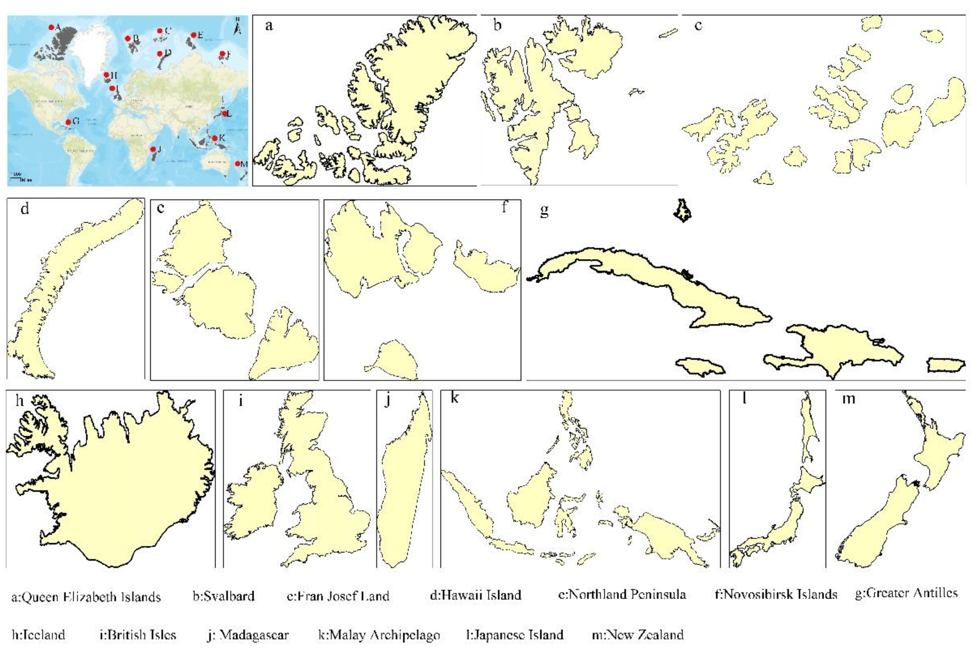
Island boundary data were selected as representative samples of free-form vector curves for experimental evaluation. Island boundaries are characterized by complex and irregular geometries, rich local details, high vertex density, and closed structures, which collectively pose significant challenges for vector curve compression and accurate reconstruction. These geometric properties are also commonly observed in other types of spatial vector line data, such as coastlines, rivers, roads, and administrative boundaries. Therefore, island boundary lines provide a suitable and representative testbed for evaluating the effectiveness and generality of the proposed compression framework. Global island boundary data were obtained from Petal Maps. The dataset includes 98 islands distributed worldwide, covering both archipelagos and individual islands, with a total boundary length of 402,776,238.59 m (Figure 4). The original vector data were preprocessed following the procedure described in Section 2.2, including curve segmentation, equidistant resampling, and normalization. After preprocessing, the dataset was transformed into 16,123 curve segments, each represented by a fixed-length feature vector derived from coordinate increments. The resulting input matrix has dimensions of 16,123 × 200, where 16,123 denotes the number of curve segments and 200 corresponds to the standardized feature length of each segment.

The convolutional autoencoder was implemented using the PyTorch deep learning framework based on the architecture described in Section 2.3.1. The network consists of an encoder and a decoder, together with input and output layers. The encoder comprises two one-dimensional convolutional layers followed by a fully connected layer, while the decoder mirrors this structure with a fully connected layer and two transposed convolutional layers. The Rectified Linear Unit (ReLU) activation function was used for all hidden layers, and the root mean square error (RMSE) was adopted as the loss function for model training. In terms of parameter configuration, the convolution kernel size was set to 1 × 7, with a stride of 5 (corresponding to half of the kernel size) and a padding of 1. The first convolutional layer contained 16 channels, and the second contained 32 channels. The learning rate was set to 0.001, and the Adam optimizer was employed to update model parameters. The network was trained for 300 epochs, after which the training loss stabilized and convergence was observed. The batch size was set to 512. The preprocessed curve segments were randomly divided into training and testing sets with a ratio of 7:3. The training set was used to optimize the network parameters through backpropagation, while the testing set was excluded from training and used exclusively for evaluating reconstruction accuracy.

3.2. Model Accuracy Analysis

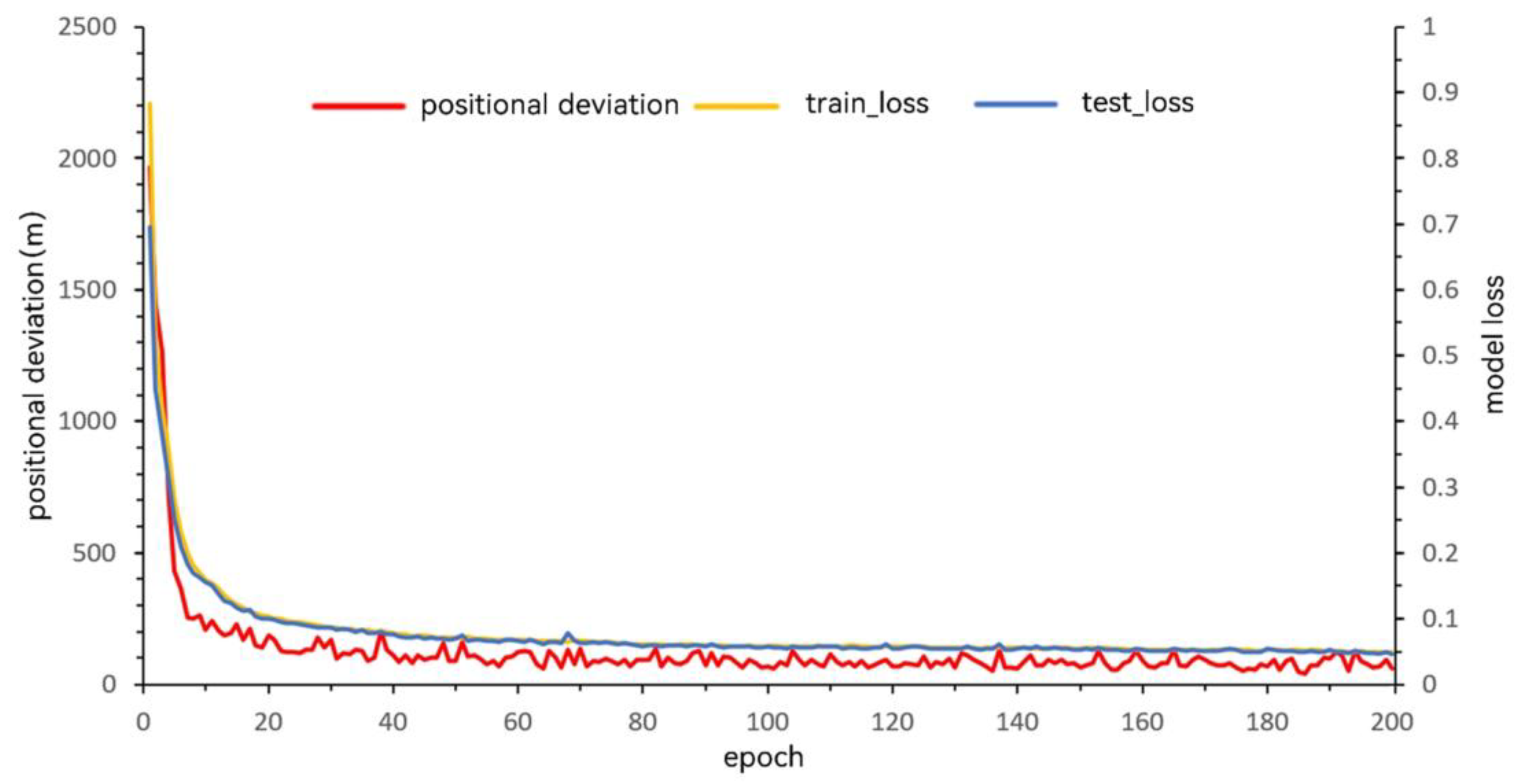
To analyze the training behavior and reconstruction performance of the proposed model, an intermediate compression level of 30% was selected as a representative example. Figure 5 illustrates the variation of model loss and mean positional deviation during the training process under this compression setting. The horizontal axis represents the number of training epochs, with each epoch corresponding to one complete forward and backward propagation over the training dataset. The right vertical axis denotes the reconstruction loss, while the left vertical axis indicates the mean positional deviation measured in meters.

As shown in Figure 5, the reconstruction loss decreases rapidly during the initial training stage, particularly within the first 20 epochs, and subsequently oscillates around a stable value, indicating that the model converges effectively. The close agreement between training and testing loss curves suggests that the model does not suffer from overfitting. A similar trend is observed for the mean positional deviation: the error decreases sharply in the early epochs and then gradually stabilizes, with only minor fluctuations observed between epochs 20 and 200. This consistency between loss convergence and positional accuracy indicates stable and reliable model training.

After training, the learned model parameters were saved and used to reconstruct island boundary segments for quantitative accuracy evaluation. To investigate the relationship between compression ratio and reconstruction accuracy, the dimensionality of the latent feature vector was set to 100, 80, 60, 40, and 20, corresponding to compression rates of 50%, 40%, 30%, 20%, and 10%, respectively. Here, the compression rate is defined as the ratio between the latent vector length and the original input vector length. For each compression setting, the decoder was applied to reconstruct the compressed features, and the mean positional deviation was computed. The reconstruction results obtained using the best-performing model parameters are summarized in Table 1.

As shown in Table 1, when the compression rate is set to 50%, 40%, or 30%, the mean positional deviation remains within the range of approximately 40–50 m. In contrast, further increasing the compression level leads to a noticeable degradation in reconstruction accuracy. At a compression rate of 20%, the mean displacement increases to 62.107 m, and at 10% compression, it rises sharply to 117.831 m. These results indicate that excessive reduction of the latent feature dimension significantly weakens the model’s ability to preserve fine-scale geometric details, resulting in increased positional distortion.

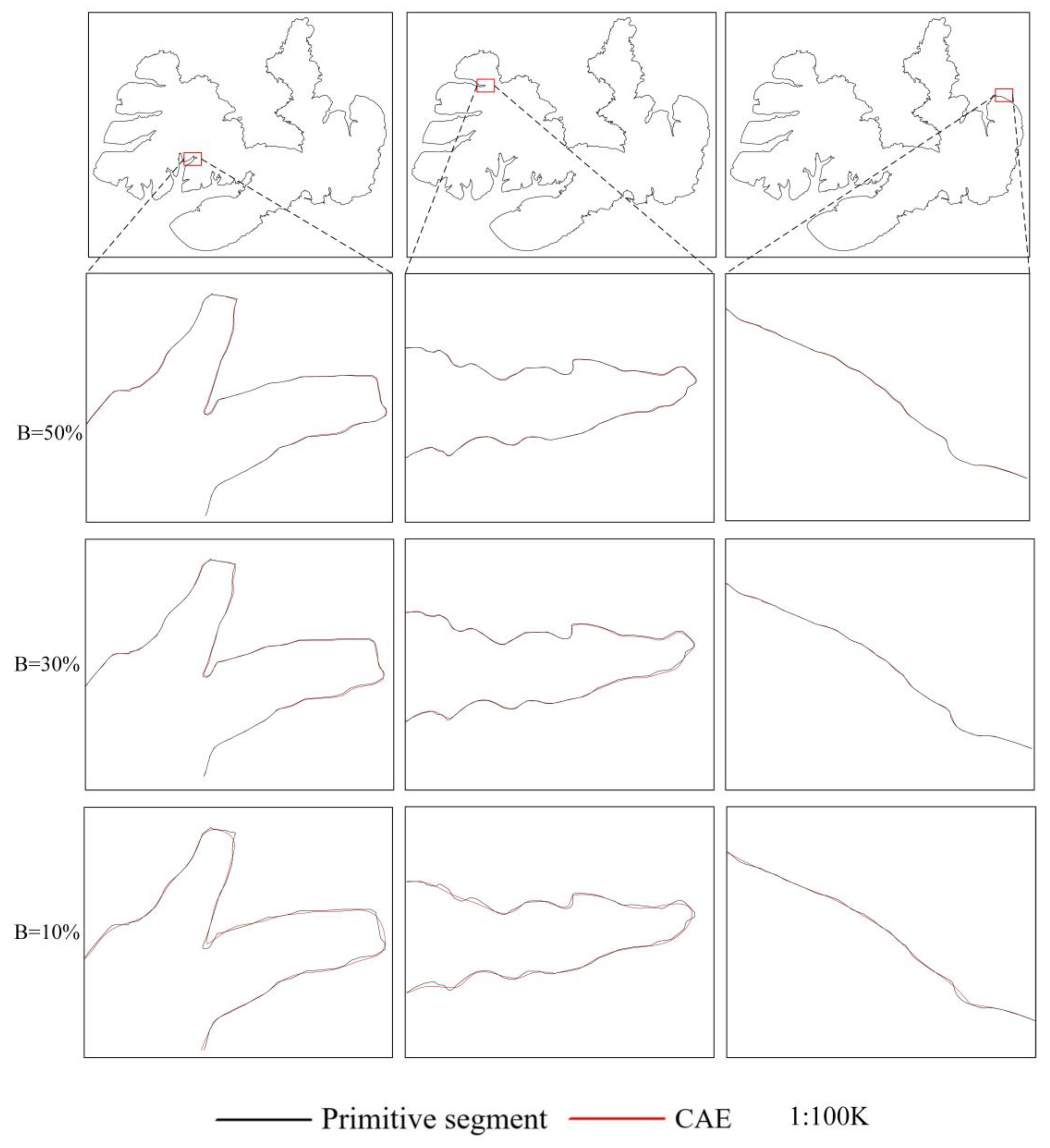
To provide a qualitative assessment of reconstruction performance, Figure 6 presents reconstructed island boundary curves at a map scale of 1:100,000 under different compression rates. At a compression rate of 50%, the reconstructed curves exhibit only minor deviations from the original boundaries, which are visually negligible. At 30% compression, local deviations become more apparent, yet the overall curve shape remains visually consistent with the original. In contrast, at a compression rate of 10%, pronounced geometric distortions can be observed, further confirming the decline in reconstruction fidelity at high compression levels. These visual results are consistent with the quantitative accuracy analysis and demonstrate the trade-off between compression efficiency and geometric accuracy.

4. Comparative Analysis with Other Methods

In this study, a convolutional autoencoder (CAE) is proposed for the compression of island boundary vector data. The encoder extracts geometric features by transforming sequences of coordinate increments into compact latent vectors, thereby achieving effective data reduction, while the decoder reconstructs the original curves from these latent representations when needed. For comparison, two alternative compression approaches were also considered. First, a fully connected autoencoder (FC-AE) was implemented by replacing the convolutional layers in the proposed model with fully connected layers, enabling an assessment of the impact of convolutional feature extraction on compression performance. Second, a Fourier series–based compression method was adopted as a classical function-fitting approach, in which curves are represented by a limited number of frequency components, yielding a low-dimensional approximation of the original geometry.

To evaluate and compare the effectiveness of these three methods, identical datasets were compressed at multiple compression rates, and reconstruction accuracy was quantitatively assessed using the mean positional deviation metric defined in Section 2.4. All methods were applied to the same preprocessed curve segments and evaluated under consistent experimental conditions to ensure a fair and objective comparison.

4.1. Fourier Series-Based Curve Compression

Island boundary line data are typically represented in the spatial domain as ordered sets of points. Fourier series expansion provides a classical transformation from the spatial domain to the frequency domain by representing a periodic function as a weighted sum of sine and cosine components with different frequencies. Under this framework, the spatial coordinates of vector line data can be interpreted as one-dimensional signals along the curve length, and the original curve geometry can be approximated by a truncated Fourier series, as expressed in Equation (6). A prerequisite for applying Fourier series approximation is that the target curve must be periodic. However, in practical experiments, the segmented island boundary lines are open curves and therefore non-periodic. To satisfy the periodicity requirement, a mirroring strategy was adopted. Specifically, each segmented arc was symmetrically mirrored with respect to its endpoints, and the mirrored curve was connected to the original segment, forming a closed curve. This procedure preserves the local geometric characteristics of the original segment while enabling Fourier series representation.

$$\left.\begin{array}{c}\mathrm{X}\left(\mathrm{s}\right)\approx {\displaystyle \frac{{\mathrm{A}}_0^{\mathrm{X}}}{2}}+{\displaystyle \sum _{\mathrm{n}=1}^{\mathrm{N}}}({\mathrm{A}}_{\mathrm{n}}^{\mathrm{X}}\mathrm{c}\mathrm{o}\mathrm{s}{\displaystyle \frac{2\mathrm{n}\mathsf{\pi }\mathrm{s}}{\mathrm{L}}}+{\mathrm{B}}_{\mathrm{n}}^{\mathrm{X}}\mathrm{s}\mathrm{i}\mathrm{n}{\displaystyle \frac{2\mathrm{n}\mathsf{\pi }\mathrm{s}}{\mathrm{L}}})\\ \mathrm{Y}\left(\mathrm{s}\right)\approx {\displaystyle \frac{{\mathrm{A}}_0^{\mathrm{Y}}}{2}}+{\displaystyle \sum _{\mathrm{n}=1}^{\mathrm{N}}}({\mathrm{A}}_{\mathrm{n}}^{\mathrm{Y}}\mathrm{c}\mathrm{o}\mathrm{s}{\displaystyle \frac{2\mathrm{n}\mathsf{\pi }\mathrm{s}}{\mathrm{L}}}+{\mathrm{B}}_{\mathrm{n}}^{\mathrm{Y}}\mathrm{s}\mathrm{i}\mathrm{n}{\displaystyle \frac{2\mathrm{n}\mathsf{\pi }\mathrm{s}}{\mathrm{L}}})\end{array}\right\}$$

(6)

Where ${\mathrm{A}}_{\mathrm{n}}^{\mathrm{X}},{\mathrm{B}}_{\mathrm{n}}^{\mathrm{X}},{\mathrm{A}}_{\mathrm{n}}^{\mathrm{Y}},\mathrm{a}\mathrm{n}\mathrm{d}{\mathrm{B}}_{\mathrm{n}}^{\mathrm{Y}}$​ denote the Fourier coefficients for the x- and y-coordinates, respectively; $\mathrm{L}$ denotes the period of the arc segment; s denotes the curve-length parameter; and $\mathrm{N}$ denotes the number of retained Fourier expansion terms. As $\mathrm{N}\to +\mathrm{\infty }$, the Fourier series can theoretically reconstruct the original curve without loss. In practice, a larger $\mathrm{N}$ yields stronger compression at the cost of geometric fidelity.

In the Fourier series–based curve compression method, the compression rate $\mathrm{B}$ is controlled by the number of retained expansion terms $\mathrm{N}$. A smaller $\mathrm{N}$ corresponds to a lower compression rate and thus a higher degree of data reduction. Assuming that the original curve contains M sampled points, the compression rate $\mathrm{B}$ can be defined as shown in Equation (7).

$$\mathrm{B}={\displaystyle \frac{4\mathrm{N}+2}{2\mathrm{M}}}\approx {\displaystyle \frac{2\mathrm{N}}{\mathrm{M}}}$$

(7)

4.2. Fully Connected Autoencoder-Based Compression

Similar to the convolutional autoencoder, the fully connected autoencoder (FCAE) adopts coordinate increment sequences as input and performs curve compression by learning a nonlinear mapping between the input space and a low-dimensional latent space. In this model, the encoder and decoder are constructed using multilayer perceptrons (MLPs), in which all neurons in adjacent layers are fully connected. Owing to the global connectivity of fully connected layers, the FCAE is capable of capturing overall structural patterns of the input sequence.

Neural networks are typically organized as multilayer architectures consisting of an input layer, multiple hidden layers, and an output layer. Each neuron receives weighted inputs from the preceding layer, applies a nonlinear activation function, and propagates the transformed signal forward. While the representational capacity of a single neuron is limited, a sufficiently deep and wide network can approximate complex nonlinear functions. In the fully connected autoencoder framework, the encoder progressively maps the coordinate increment sequence into a compact latent vector through a series of fully connected hidden layers, and the decoder reconstructs the original sequence from this latent representation in a symmetric manner.

Compared with convolutional architectures, the fully connected autoencoder does not employ local receptive fields or parameter sharing. As a result, it generally involves a larger number of trainable parameters and higher computational cost for inputs of the same dimensionality. Moreover, because spatial locality is not explicitly modeled, local geometric continuity along the curve may be less effectively preserved than in convolution-based models. Nevertheless, the fully connected autoencoder provides a meaningful baseline for evaluating the advantages of convolutional structures in vector curve compression. For a fair comparison with the convolutional autoencoder, the compression ratio of the fully connected autoencoder is defined in the same manner as in Equation (3), based on the dimensionality of the latent vector relative to the input sequence length.

4.3. Comparative Results and Discussion

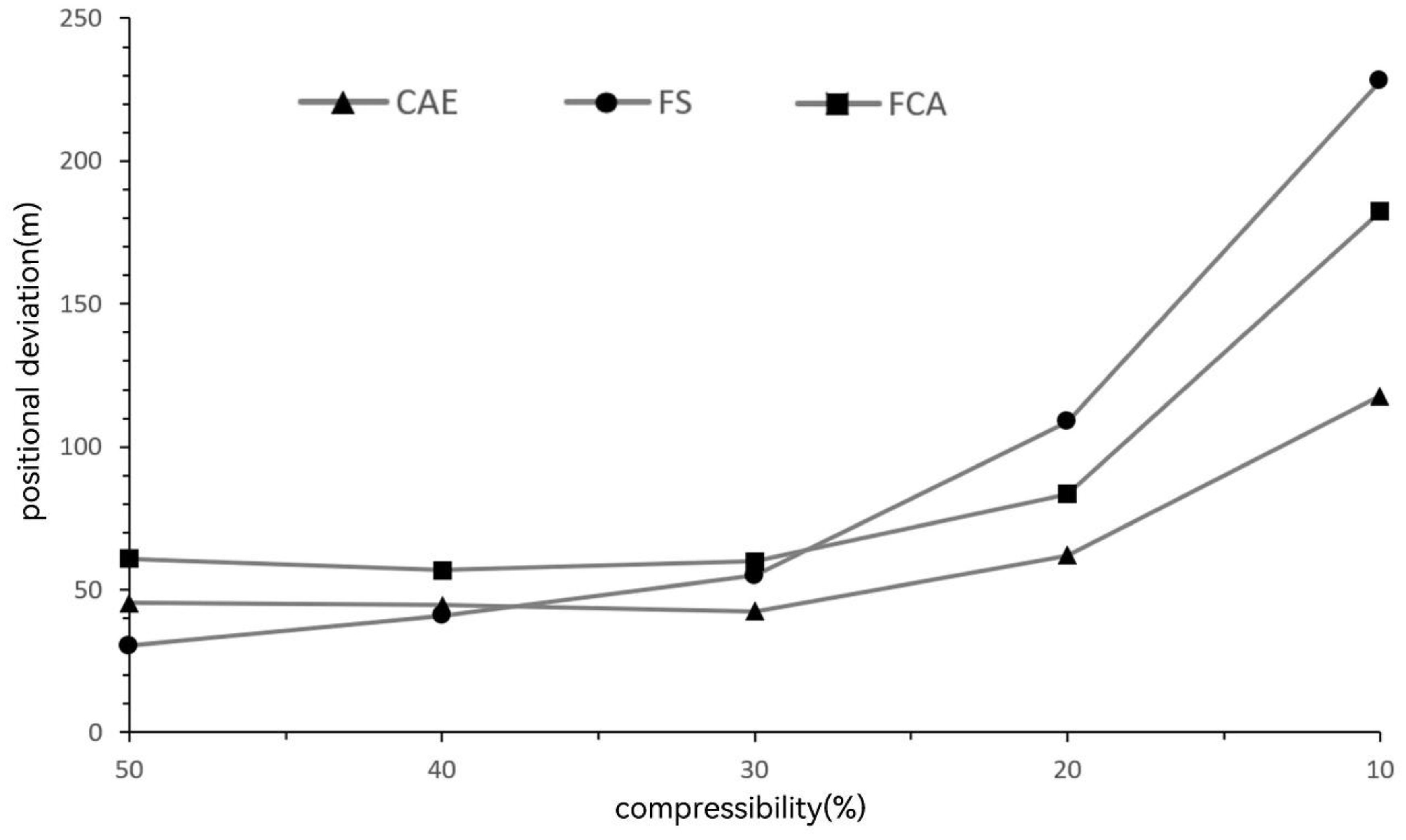
To evaluate the performance of different curve compression strategies, the island boundary dataset described in Section 3.1 was compressed using three methods: the proposed convolutional autoencoder (CAE), the Fourier series-based method (FS), and the fully connected autoencoder (FCAE). Reconstruction accuracy under varying compression ratios is quantitatively compared in Figure 7 using the mean point displacement metric defined in Section 2.4.

The results indicate that when the compression ratio is relatively high (50% and 40%), the Fourier series method achieves slightly lower mean displacement errors than the convolutional autoencoder. This behavior can be attributed to the strong representation capability of low-frequency Fourier components for smooth and slowly varying curves. However, as the compression ratio decreases (30% and below), the reconstruction accuracy of the Fourier series method deteriorates rapidly, whereas the convolutional autoencoder maintains relatively stable performance. Under these lower compression ratios, the convolutional autoencoder consistently outperforms the Fourier series approach, demonstrating superior robustness in high-compression scenarios. Across all tested compression ratios, the convolutional autoencoder achieves lower reconstruction errors than the fully connected autoencoder.

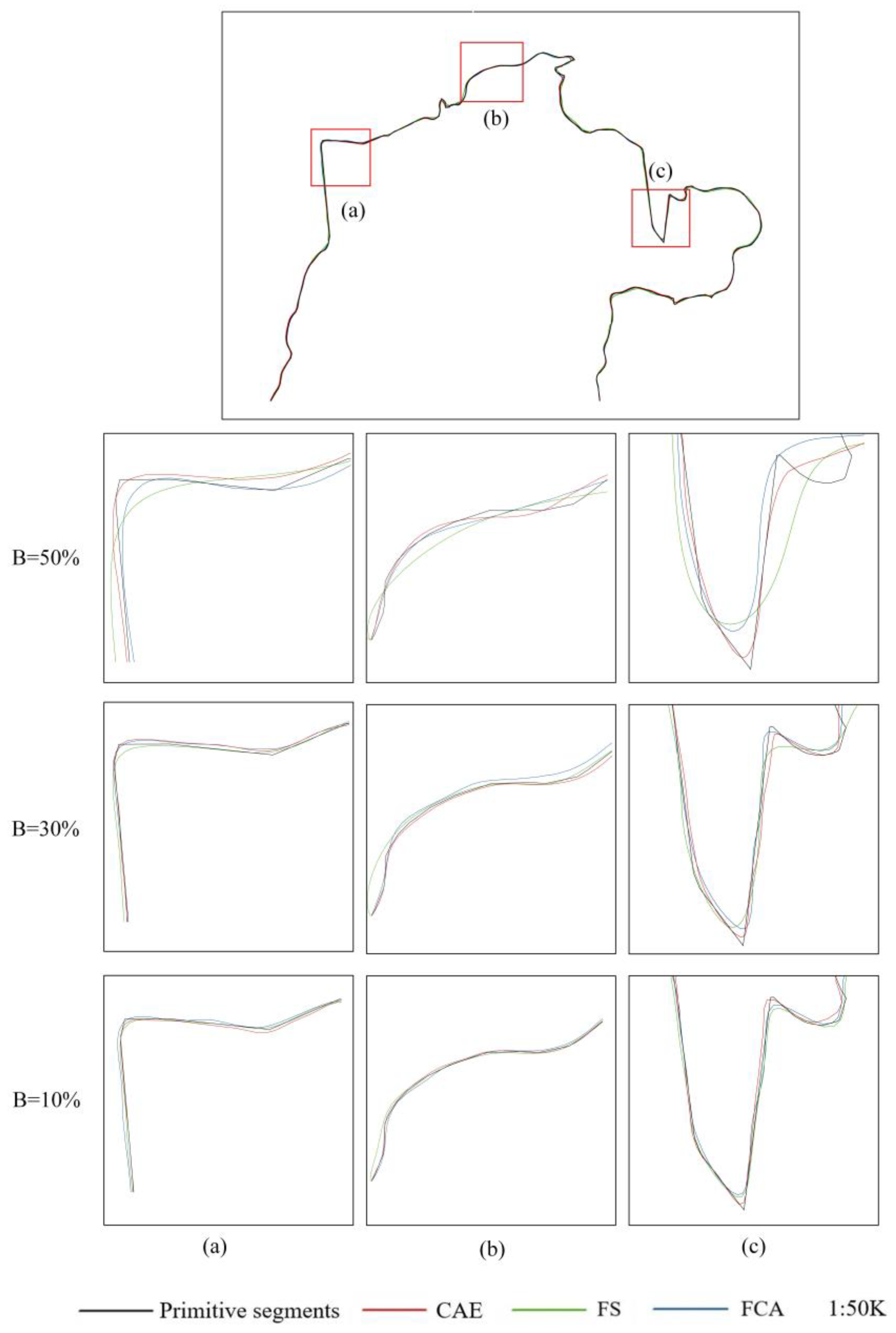
Figure 8 provides a visual comparison of reconstructed island boundary curves at compression ratios of 50%, 30%, and 10%, displayed at a map scale of 1:50,000. Each row compares the three methods under the same compression ratio, while each column illustrates the effect of different compression levels for the same geographic region. The original curve is shown in black, while reconstructions generated by the convolutional autoencoder (CAE), Fourier series method (FS), and fully connected autoencoder (FCAE) are shown in red, green, and blue, respectively. To highlight structural differences, three representative curve types—flat, concave, and convex—were selected for visualization.

At a moderate compression ratio of 50%, all three methods are able to reconstruct island boundaries with relatively small deviations from the original curves, and visual differences are generally subtle. As the compression ratio decreases to 30% and further to 10%, reconstruction errors become increasingly pronounced. In particular, under high compression (10%), the convolutional autoencoder consistently produces reconstructed curves that remain closest to the original geometry across all curve types. This advantage is evident not only for flat segments but also for concave and convex structures, which contain more complex local geometric variations.

In contrast, the fully connected autoencoder exhibits larger deviations, especially in regions with rapid directional changes, suggesting limited effectiveness in preserving local geometric continuity. The Fourier series method remains competitive for relatively flat curves but shows substantial degradation when reconstructing concave and convex shapes under high compression, as higher-frequency components required to represent local curvature are progressively discarded. These observations highlight the ability of the convolutional autoencoder to balance global structure and local feature preservation through localized convolutional operations and shared parameters, making it more suitable for high-efficiency compression of complex vector curves.

5. Analysis and Discussion

5.1. Geometric Scale Sensitivity of the Convolutional Autoencoder

In convolutional neural networks (CNNs), overall performance is jointly determined by network architecture, layer configuration, and hyperparameter selection. Among these components, the convolutional kernel plays a central role in feature extraction by defining the size of the local receptive field. Through element-wise multiplication and summation with the input signal, convolutional kernels capture localized patterns, and their sliding operation aggregates such local features into higher-level representations. For one-dimensional sequential data, such as coordinate increment sequences used in this study, kernel size determines the geometric scale at which local variations along the curve are perceived by the model. From a geographic perspective, this process can be interpreted as analogous to the progressive scanning and abstraction of spatial features in cartographic generalization, where local geometric details are perceived within a limited contextual window. If the receptive field is too small, the kernel may fail to capture meaningful shape patterns beyond minor point-to-point fluctuations; if it is too large, fine-scale geometric variations may be overly smoothed or obscured. Therefore, an appropriate kernel size is essential for balancing sensitivity to local geometry and robustness to noise.

To examine the influence of kernel size on compression performance, a series of experiments were conducted using kernel sizes of {4, 7, 9, 11, 13} under a fixed compression rate of 30%. Reconstruction accuracy was evaluated using the mean positional deviation metric defined in Section 2.4. The results are summarized in Table 2. Among the tested configurations, a kernel size of 1×7 achieved the lowest mean positional deviation, indicating the most effective balance between local feature extraction and geometric continuity preservation under the current experimental setup.

It should be emphasized that this result does not imply a universally optimal kernel size for all types of vector curve data. Rather, the observed performance reflects an empirical alignment between the kernel receptive field and the characteristic geometric scale of the input curves after segmentation and resampling. For other vector line datasets with different geometric complexity, sampling density, or segmentation strategies, the optimal kernel size may vary accordingly. Nonetheless, these results demonstrate that moderate kernel sizes, which capture short-range geometric dependencies without excessively expanding the receptive field, are generally well suited for learning compact representations of vector curve data in compression tasks.

5.2. Effect of Segment Length on Compression Stability and Accuracy

Segment length determines the geometric extent of curve information presented to the autoencoder at each training instance and therefore has a direct impact on representation learning and reconstruction accuracy. From a modeling perspective, segment length controls the balance between geometric completeness and structural variability: shorter segments emphasize fine-scale local details, whereas longer segments incorporate broader contextual shape information but also introduce greater morphological complexity. To investigate the influence of segment length on compression performance, four segment lengths—15 km, 25 km, 50 km, and 75 km—were evaluated under a fixed compression rate of 30%. Reconstruction accuracy was assessed using the mean positional deviation metric described in Section 2.4. The experimental results are summarized in Table 3. As shown in Table 3, reconstruction accuracy improves as the segment length increases from 15 km to 25 km, indicating that very short segments may not contain sufficient geometric context for the autoencoder to effectively learn characteristic curve patterns. When the segment length is further increased to 50 km and 75 km, however, reconstruction accuracy deteriorates noticeably. This decline suggests that overly long segments introduce excessive geometric variability, making it more difficult for the model to encode diverse shape patterns into a fixed-length latent representation without loss of detail.

These results indicate the existence of an intermediate segment length that provides an effective trade-off between geometric representativeness and model learnability. In the present experimental configuration, a segment length of approximately 25 km yields the lowest mean positional deviation and thus represents an empirically suitable choice. It should be noted that this value is not intended to serve as a universal optimal length for all vector line datasets. Instead, it reflects a dataset- and model-dependent balance between local geometric continuity and global shape complexity. For other types of vector curves or different sampling densities, the optimal segment length may vary accordingly. Nevertheless, the observed trend highlights the importance of aligning segment length with the representational capacity of the autoencoder when designing compression frameworks for vector curve data.

5.3. Compression Rate Recommendations for Multi-Scale Island Visualization

Reconstruction of vector curves using the decoder inevitably introduces geometric deviations from the original data, and these deviations generally increase as the compression rate rises. As demonstrated in Table 1, higher compression ratios lead to larger mean positional deviations. In practical cartographic applications, however, the acceptability of such deviations depends not only on their absolute magnitude in ground units but also on the target map scale and the limits of human visual perception.

In cartography and map visualization, it is widely recognized that positional deviations smaller than approximately 0.2 mm on a printed or displayed map are difficult for human observers to reliably perceive under typical viewing conditions. This empirical threshold is commonly adopted as a practical criterion for evaluating geometric accuracy in multi-scale mapping. By converting this map-space tolerance into ground-space distances for different map scales, acceptable deviation thresholds can be derived and used to guide compression rate selection. Table 4 summarizes the recommended compression rates for vector curve data at different map scales based on this visual discernibility criterion. For large-scale maps (1:100K and finer), even relatively small positional deviations in ground space may exceed the visual tolerance, indicating that aggressive compression is not suitable in such contexts. At medium to small scales, however, the allowable ground displacement increases substantially, making higher compression rates feasible without introducing perceptible visual distortion. Specifically, for map scales around 1:250K, a compression rate of approximately 30% satisfies the visual accuracy requirement, while at 1:500K the compression rate can be further reduced to about 20%. For small-scale representations such as 1:1M, compression rates as low as 10% remain visually acceptable. These results demonstrate that compression rate selection should be scale-dependent and that substantial storage savings can be achieved at smaller map scales without compromising visual fidelity.

It should be emphasized that the recommended compression rates reported here are derived from empirical experiments under the current model configuration and dataset characteristics. While the specific numerical values may vary for different vector curve types or modeling strategies, the underlying principle—that compression decisions should be jointly guided by reconstruction accuracy and target visualization scale—remains generally applicable. This scale-aware compression strategy provides a practical framework for integrating deep learning–based vector data compression into multi-scale geographic information systems.

6. Conclusions and Future Work

This study proposes a convolutional autoencoder–based framework for the compression of vector curve data and demonstrates its effectiveness through systematic experiments on complex free-form geometries. By transforming coordinate sequences into coordinate-increment representations, the proposed encoder learns compact latent vectors that preserve essential geometric characteristics, while the decoder reconstructs curves with high positional fidelity. Experimental results confirm that the proposed approach achieves a favorable balance between compression efficiency and reconstruction accuracy. The trained encoder–decoder parameters are shared and amortized across a large number of curve segments and therefore do not scale with dataset size, making the proposed approach suitable for storage-oriented compression scenarios.

Comparative analyses with Fourier series–based compression and fully connected autoencoders indicate that the convolutional autoencoder provides consistently superior performance across a wide range of compression ratios. While frequency-domain methods may achieve slightly higher accuracy at relatively low compression levels, the proposed method exhibits clear advantages under moderate to high compression, where nonlinear local geometric features become more difficult to preserve using traditional parametric representations. The results further demonstrate that convolutional structures are more effective than fully connected architectures in capturing local geometric continuity in vector curve data. Through a series of sensitivity analyses, this study highlights the importance of scale alignment between model design, data representation, and application requirements. The experiments reveal that both the receptive field of convolutional kernels and the geometric extent of curve segments significantly influence reconstruction performance, and that intermediate scales yield the most effective trade-offs between representational capacity and model stability. In addition, by linking reconstruction accuracy to cartographic visual tolerance, a scale-aware compression strategy is established, providing practical guidance for selecting compression rates in multi-scale map visualization scenarios. The proposed method is particularly suitable for small- and medium-scale mapping applications, where substantial data reduction can be achieved without perceptible visual degradation.

Despite these promising results, several limitations remain. The experimental evaluation focuses on a single category of vector curves, and the current framework emphasizes geometric reconstruction without explicitly modeling topological consistency or semantic attributes. Future work will extend the proposed approach to a broader range of vector datasets, including transportation networks and hydrographic features, and will investigate topology-aware constraints and multi-task learning strategies to further improve reconstruction robustness and generalization. In addition, integrating adaptive segmentation and scale-aware model configurations represents a promising direction for enhancing the flexibility of deep learning–based vector data compression in real-world geographic information systems.

References

- Douglas, D.H.; Peucker, T.K. Algorithms for the reduction of the number of points required to represent a digitized line or its caricature. Cartographica 1973, 10, 112–122. [CrossRef]
- Yang, D.; Wang, J.; Lv, G. Study of realization method and improvement of Douglas–Peucker algorithm of vector data compressing. Bull. Surv. Mapp. 2002, 7, 18–19, 22.
- Li, C.; Luo, W.; Chen, G.; Yan, W. Discussion on the progressive improved algorithm for cartographic generalization of line features. Sci. Surv. Mapp. 2015, 40, 123–126.
- Yu, J.; Chen, G.; Zhang, X. An improved Douglas–Peucker algorithm aimed at simplifying natural shoreline into direction-line. In Proceedings of the 21st International Conference on Geoinformatics; IEEE: Kaifeng, China, 2013; pp. 1–5.
- Wu, F.; Deng, H. Using genetic algorithms for solving problems in automated line simplification. Acta Geod. Cartogr. Sin. 2003, 32, 349–355.
- Li, Z.; Openshaw, S. Algorithms for automated line generalization based on a natural principle of objective generalization. Int. J. Geogr. Inf. Syst. 1992, 6, 373–389. [CrossRef]
- Liu, P.; Ai, T.; Bi, X. Multi-scale representation model for contour based on Fourier series. Geom. Inf. Sci. Wuhan Univ. 2013, 38, 221–224.
- Liu, P.; Li, X.; Liu, W.; Ai, T. Fourier-based multi-scale representation and progressive transmission of cartographic curves on the Internet. Cartogr. Geogr. Inf. Sci. 2015, 43, 454–468. [CrossRef]
- Liu, P.; Xiao, T.; Xiao, J.; Ai, T. A head–tail information break method oriented to multi-scale representation of polyline. Acta Geod. Cartogr. Sin. 2020, 49, 921–933.
- Liu, P.; Xiao, T.; Xiao, J.; Ai, T. A multi-scale representation model of polyline based on head/tail breaks. Int. J. Geogr. Inf. Sci. 2020, 34, 2275–2295. [CrossRef]
- Wu, F.; Zhu, G. Multi-scale representation and automatic generalization of relief based on wavelet analysis. Geom. Inf. Sci. Wuhan Univ. 2001, 26, 170–176.
- Wu, F. Scaleless representations for polyline spatial data based on wavelet analysis. Geom. Inf. Sci. Wuhan Univ. 2004, 29, 488–491.
- Du, J.; Wu, F.; Yin, J.; Liu, C.; Gong, X. Polyline simplification based on the artificial neural network with constraints of generalization knowledge. Cartogr. Geogr. Inf. Sci. 2022, 49, 313–337. [CrossRef]
- Jiang, B.; Xu, S.; Wu, Y.; Wang, M. Automatic vector polyline simplification based on region proposal network. Acta Geod. Cartogr. Sin. 2023, 52, 2209–2222.
- Courtial, A.; El Ayedi, A.; Touya, G.; Zhang, X. Exploring the potential of deep learning segmentation for mountain roads generalisation. ISPRS Int. J. Geo-Inf. 2020, 9, 338. [CrossRef]
- Du, J.; Wu, F.; Xing, R.; Gong, X.; Yu, L. Segmentation and sampling method for complex polyline generalization based on a generative adversarial network. Geocarto Int. 2021, 37, 4158–4180. [CrossRef]
- Yu, W.; Chen, Y. Data-driven polyline simplification using a stacked autoencoder-based deep neural network. Trans. GIS 2022, 26, 2302–2325. [CrossRef]
- Yan, X.; Yang, M. A deep learning approach for polyline and building simplification based on graph autoencoder with flexible constraints. Cartogr. Geogr. Inf. Sci. 2023, 51, 79–96. [CrossRef]
- Liu, P.; Ma, H.; Zhou, Y.; Shao, Z. Autoencoder neural network method for curve data compression. Acta Geod. Cartogr. Sin. 2024, 53, 1634–1643.
- Lawrence, S.; Giles, C.L.; Tsoi, A.C.; Back, A.D. Face recognition: A convolutional neural network approach. IEEE Trans. Neural Netw. 1997, 8, 98–113. [CrossRef]
- Hinton, G.E.; Salakhutdinov, R.R. Reducing the dimensionality of data with neural networks. Science 2006, 313, 504–507. https://doi.org10.1126/science.1127647.
- National Oceanic and Atmospheric Administration. Cartographic Generalization and Symbolization. NOAA Technical Report NOS 127 CGS 12; NOAA Office of Coast Survey: Washington, DC, USA, 2009.