Submitted:
23 December 2025
Posted:
24 December 2025
You are already at the latest version
Abstract
Groundwater resources in semi-arid and industrial regions are increasingly threatened by unsustainable extraction, groundwater contamination, and climate-induced variability. Tiruppur District in Tamil Nadu, India, represents a critical case where rapid industrial growth, intensive agricultural activity, and changing climatic patterns have resulted in severe groundwater stress. This study proposes a hybrid artificial intelligence–based framework for the assessment and forecasting of groundwater levels and quality under climate change conditions. The framework integrates multi-source datasets comprising historical groundwater level records (1994–2024), groundwater quality parameters, and meteorological data. To address the non-stationary nature of hydrological time series, Improved Complete Ensemble Empirical Mode Decomposition with Adaptive Noise (ICEEMDAN) and Variational Mode Decomposition (VMD) are employed prior to model training. Deep learning models, including Slime Mould Algorithm–optimized Long Short-Term Memory (SMA–LSTM) networks and CNN–LSTM hybrids, are developed to capture temporal and spatial dependencies. An Adaptive Weighting Model is used to ensemble predictions and improve robustness. Model performance is evaluated using Mean Absolute Error, Root Mean Square Error, Coefficient of Determination, and Nash–Sutcliffe Efficiency. The proposed ensemble framework demonstrates superior predictive accuracy, achieving an R² value of 0.948 and an NSE of 0.938. The results confirm the effectiveness of hybrid deep learning approaches for climate-resilient groundwater management and highlight their scalability to other water-stressed regions.
Keywords:
groundwater forecasting
; climate change
; deep learning
; LSTM
; signal decomposition
; ensemble learning
1. Introduction
Groundwater is a critical freshwater resource supporting domestic supply, agricultural irrigation, and industrial production worldwide. In semi-arid regions, groundwater often constitutes the primary source of water due to limited and unreliable surface water availability. In India, rapid population growth, urbanization, and industrial expansion have significantly increased groundwater abstraction, leading to widespread declines in groundwater levels and deterioration of groundwater quality.
Climate change has emerged as a major driver of groundwater stress through altered precipitation regimes, increased evapotranspiration, and a higher frequency of extreme hydrological events. These processes directly affect recharge dynamics and exacerbate groundwater depletion, particularly in hard-rock aquifer systems that exhibit limited storage capacity and strong dependence on episodic rainfall [5]. Recent studies across the Indian peninsula have demonstrated strong linkages between groundwater level fluctuations and climate variability indices, emphasizing the need to incorporate climate signals into groundwater assessment and prediction frameworks [3].
Traditional groundwater forecasting approaches based on statistical or physically based models often struggle to capture the nonlinear and non-stationary behavior induced by the combined effects of climate variability and anthropogenic pressure. Consequently, machine learning and deep learning techniques have gained increasing attention for groundwater level prediction. Among these, Long Short-Term Memory (LSTM) networks have shown promising results due to their ability to model temporal dependencies. However, standalone LSTM models may exhibit reduced performance when applied to highly non-stationary groundwater time series.
To address this limitation, recent research has focused on integrating signal decomposition techniques with deep learning models. Hybrid frameworks combining empirical mode decomposition, wavelet analysis, and LSTM architectures have been shown to improve forecasting accuracy by isolating intrinsic temporal components prior to model training [6]. More recently, ensemble deep learning models incorporating secondary modal decomposition and multi-source data fusion have demonstrated enhanced robustness and predictive performance in groundwater level prediction [1].
In parallel, advances in groundwater monitoring infrastructure, including IoT-enabled and telemetry-based observation systems, have facilitated the availability of high-resolution temporal data, further supporting the application of data-driven prediction models [2]. At the same time, novel deep learning architectures, such as hybrid temporal convolutional network (TCN)–LSTM models with attention mechanisms, have been explored to improve feature representation and long-term dependency learning in groundwater forecasting tasks [4].
Despite these advances, there remains a need for integrated frameworks that simultaneously address non-stationarity, exploit spatial–temporal learning, and enhance prediction robustness under climate variability. This study addresses this gap by proposing a hybrid groundwater forecasting framework that combines ICEEMDAN- and VMD-based signal decomposition, optimized deep learning models, and adaptive ensemble learning for climate-resilient groundwater prediction in Tiruppur District, Tamil Nadu, India.
2. Materials and Methods
2.1. Study Area
The study area comprises Tiruppur District, situated in the western part of Tamil Nadu, India, between approximately 11.0°–11.5° N latitude and 77.0°–77.6° E longitude. The district lies within a semi-arid climatic zone, characterized by high inter-annual rainfall variability, frequent dry spells, and increasing temperature trends. Average annual rainfall is primarily governed by the southwest and northeast monsoons, with recharge largely concentrated during short, intense precipitation events.
Hydro-geologically, Tiruppur is dominated by hard-rock formations, mainly consisting of weathered and fractured crystalline rocks. Groundwater occurrence in such terrains is highly heterogeneous and is largely confined to shallow weathered zones and deeper fracture networks. The limited storage capacity of these aquifers, coupled with low natural recharge rates, makes groundwater availability extremely sensitive to variations in rainfall intensity, duration, and seasonal distribution. Consequently, groundwater levels exhibit pronounced temporal fluctuations and spatial variability across the district.
Tiruppur is internationally recognized as the “Knitwear Capital of India”, hosting a dense concentration of textile dyeing and processing industries. Rapid industrialization, combined with urban expansion and agricultural water demand, has led to persistent over-extraction of groundwater for industrial, domestic, and irrigation purposes. In the absence of perennial surface water sources, groundwater remains the primary source of water supply, further intensifying stress on aquifer systems.
In addition to quantitative depletion, groundwater quality deterioration has emerged as a critical concern. Discharge of untreated or partially treated textile effluents, rich in dissolved salts and chemical residues, has resulted in elevated levels of Total Dissolved Solids (TDS), electrical conductivity, and salinity in several parts of the district. These impacts are exacerbated by reduced dilution during low-recharge periods, particularly under prolonged drought conditions.
Climate change further compounds groundwater vulnerability in the region by altering monsoon patterns, increasing evapotranspiration, and amplifying the frequency of extreme hydrological events. These combined hydrogeological, industrial, and climatic factors make Tiruppur District a representative and high-risk case study for evaluating advanced, data-driven groundwater forecasting methodologies. The complex and non-stationary nature of groundwater dynamics in this region provides an ideal testbed for assessing the effectiveness of hybrid deep learning models under climate-induced stress conditions.
Figure 1.
Spatial distribution of the comprehensive groundwater monitoring network in Tiruppur District.
Figure 1.
Spatial distribution of the comprehensive groundwater monitoring network in Tiruppur District.
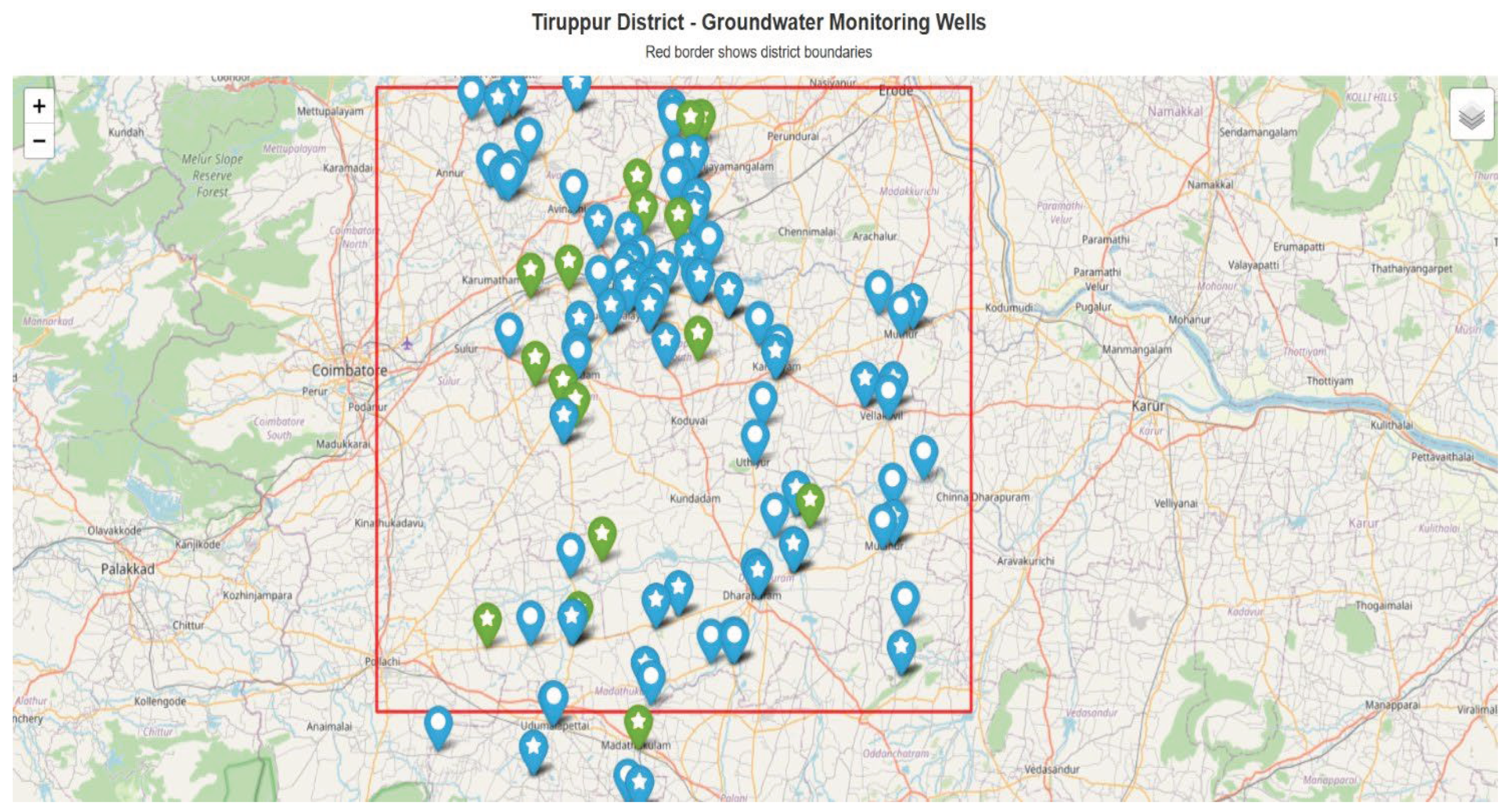
The map illustrates the locations of groundwater monitoring wells operated by the Central Ground Water Board (CGWB) and State agencies, including both manual and telemetry-based observation wells. The red boundary indicates the district extent.
Figure 2.
Block-wise distribution of groundwater monitoring wells in Tiruppur District.
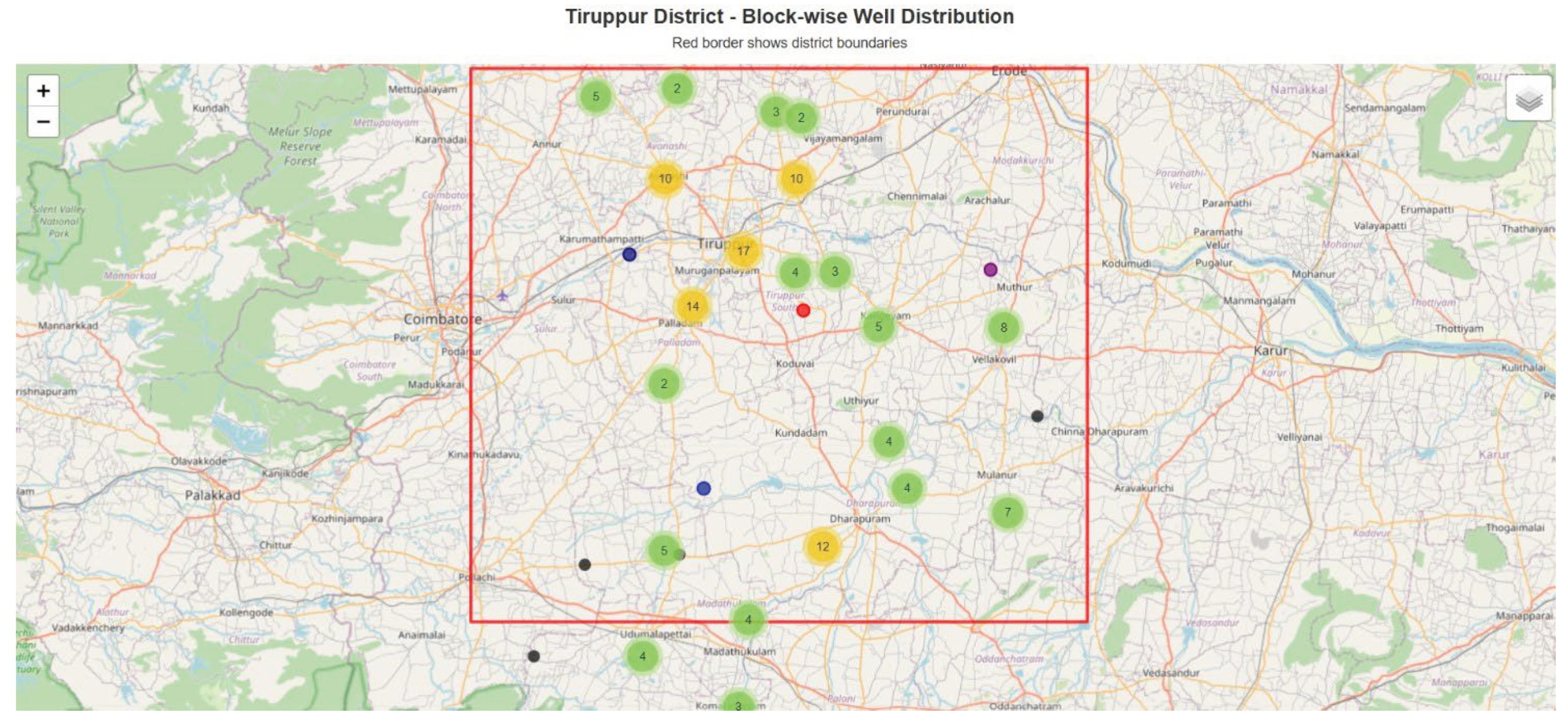
The figure shows the spatial density of monitoring wells across administrative blocks, highlighting variations in monitoring coverage within the district boundary.
Figure 3.
Distribution of telemetry-based groundwater monitoring wells in Tiruppur District.
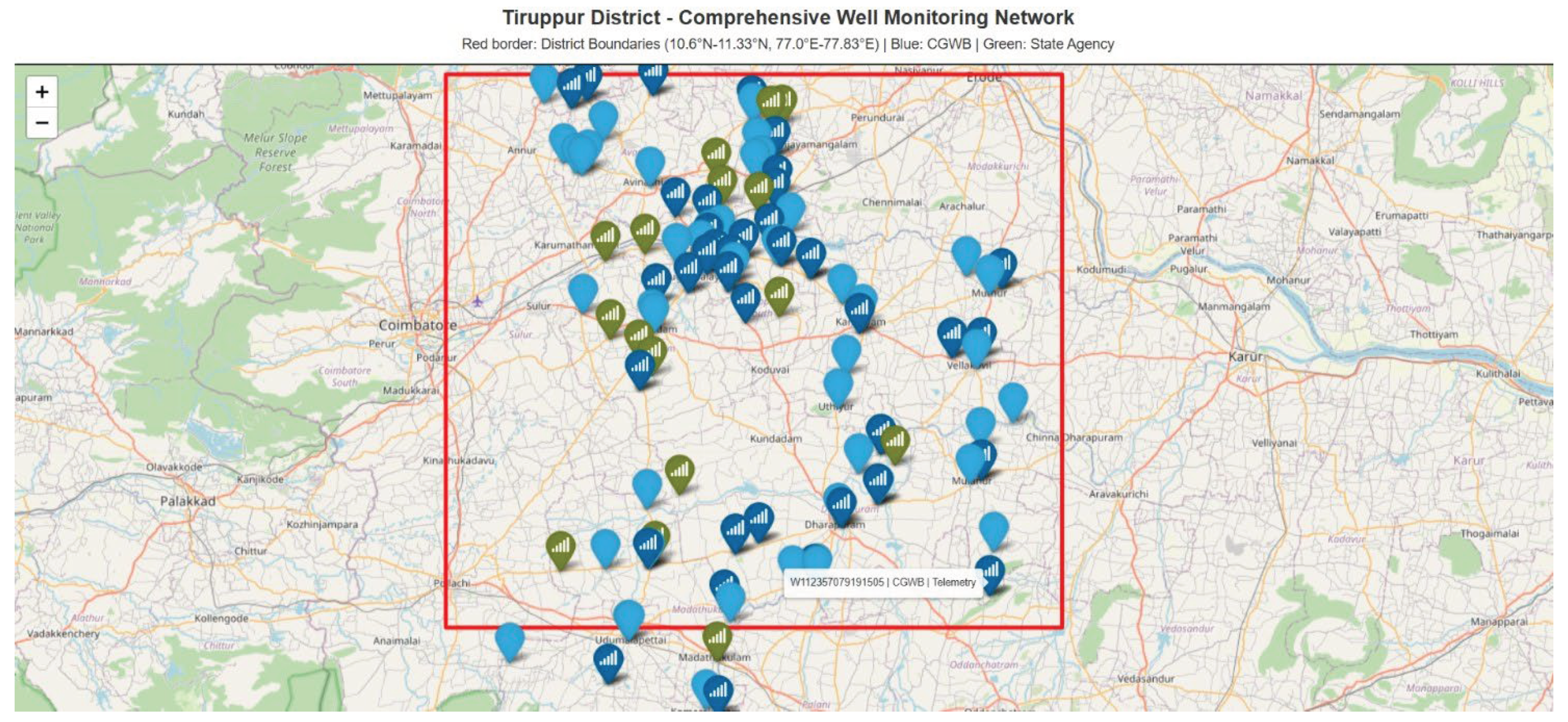
The figure highlights the spatial locations of real-time groundwater observation wells operated by monitoring agencies, supporting high-resolution temporal analysis.
2.2. Data Collection and Sources
The increasing deployment of real-time groundwater monitoring systems has enabled the collection of high-frequency groundwater level data suitable for data-driven modeling approaches. In recent years, IoT-based and telemetry-enabled groundwater observation networks have been successfully utilized to support machine learning–based groundwater level prediction [2]. In this study, groundwater level and quality data from both manual and telemetry-based monitoring wells operated by central and state agencies were integrated with meteorological observations to ensure comprehensive spatial and temporal coverage.
2.2.1. Groundwater Level Data
Groundwater level data were obtained from the Water Resources Department (WRD), Government of Tamil Nadu, covering a continuous period from 1994 to 2024. The dataset consists of monthly observations of depth to groundwater level (meters below ground level) collected from a network of observation wells distributed across Tiruppur District. Each record is accompanied by spatial attributes, including well identification number, geographic coordinates (latitude and longitude), administrative boundaries (taluk and village), and well type (dug wells and bore wells).
This long-term dataset captures seasonal recharge patterns, inter-annual variability, and long-term depletion trends driven by industrial abstraction and land-use change. The extended temporal coverage makes the dataset particularly suitable for deep learning–based time-series modeling and for assessing non-stationary groundwater behavior under evolving climatic conditions.
2.2.2. Groundwater Quality Data
Groundwater quality data were collected from the Tamil Nadu Water Supply and Drainage (TWAD) Board and the Central Ground Water Board (CGWB) for the period 2017–2023. The dataset includes key physicochemical parameters that indicate groundwater suitability for domestic and agricultural use, such as pH, electrical conductivity (EC), and total dissolved solids (TDS). In addition, major ionic constituents—including calcium (Ca), magnesium (Mg), sodium (Na), chloride (Cl), sulfate (SO), and bicarbonate (HCO)—were considered.
Derived indices such as Sodium Adsorption Ratio (SAR) and Residual Sodium Carbonate (RSC) were computed to assess salinity hazards and irrigation suitability. These parameters provide critical insight into groundwater quality degradation resulting from industrial effluent discharge, excessive abstraction, and reduced natural dilution during low-recharge periods. The inclusion of groundwater quality data allows the proposed framework to evaluate both quantitative and qualitative aspects of groundwater sustainability.
2.2.3. Meteorological and Climate Data
Meteorological data were obtained from the Indian Meteorological Department (IMD) and include daily observations of rainfall (mm), maximum and minimum temperature (°C), and relative humidity (%) for the period 1994–2024. These variables are key climatic drivers influencing groundwater recharge, evapotranspiration, and seasonal water-level fluctuations. Daily records were aggregated to a monthly temporal resolution to ensure consistency with groundwater observations.
To assess future groundwater behavior under climate change, climate projection data from the Coupled Model Intercomparison Project Phase 6 (CMIP6) were incorporated. Projections were considered under multiple Shared Socioeconomic Pathways (SSPs), including SSP2-4.5 (moderate emissions) and SSP5-8.5 (high emissions) scenarios. These datasets provide downscaled estimates of future precipitation and temperature patterns and enable long-term groundwater forecasting under alternative climate trajectories.
2.2.4. Data Integration and Temporal Alignment
All datasets were harmonized by resampling to a common monthly temporal resolution and aligned spatially using geographic coordinates. This integration facilitates seamless fusion of groundwater, quality, and climatic variables within the modeling framework.
- Groundwater Level Dataset - WRD, Tamilnadu - https://www.tn.gov.in/dept_profile.php?dep_id=NDQ=
- Groundwater Quality Dataset - TWAD, CGWB - https://cgwb.gov.in/en
- Metrological Data - IMD - https://mausam.imd.gov.in/
- Climate Projections - CMIP6 - https://www.worldclim.org/data/index.html
A summary of the datasets, sources, temporal coverage, and parameters is presented in Table 1.
Figure 4.
Overall architecture of the proposed hybrid groundwater forecasting framework.
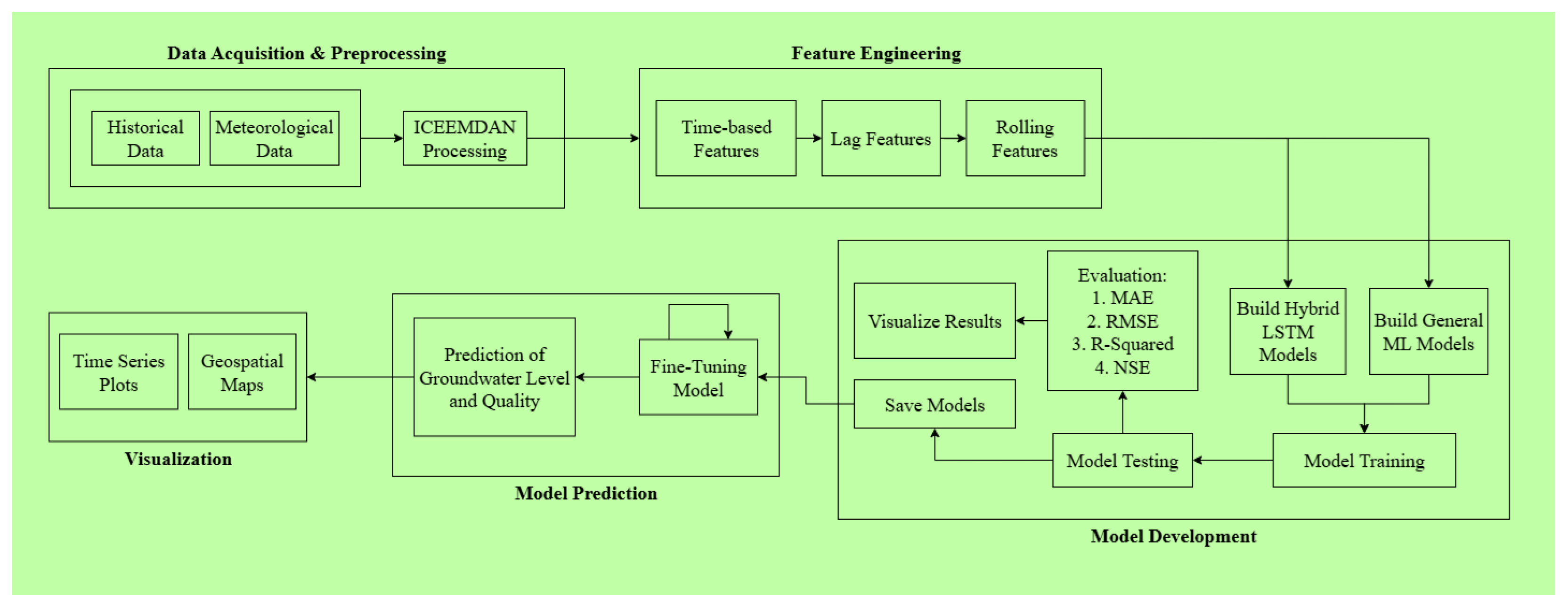
Schematic representation of the integrated framework illustrating data acquisition, preprocessing, signal decomposition, deep learning model development, adaptive ensemble learning, and forecast visualization.
2.3. Data Preprocessing and Cleaning
Data preprocessing is a critical step in developing reliable machine learning and deep learning models, particularly when working with heterogeneous hydroclimatic datasets characterized by missing values, measurement noise, and temporal inconsistencies. In this study, a comprehensive preprocessing pipeline was implemented to ensure data quality, consistency, and suitability for advanced time-series modeling.
2.3.1. Handling Missing and Invalid Data
Groundwater level and quality datasets contained missing observations due to intermittent monitoring, inaccessible wells, or instrument malfunction. Missing values in continuous time-series records were addressed using linear interpolation and forward-filling techniques, ensuring continuity while preserving temporal trends. Records containing non-numeric or invalid entries (e.g., “dry well” or “blocked”) were identified and either encoded appropriately or removed based on data completeness criteria. This approach minimized information loss while preventing the introduction of artificial bias.
2.3.2. Temporal Resampling and Alignment
To enable seamless integration of groundwater, quality, and meteorological datasets, all variables were resampled to a monthly temporal resolution. Daily meteorological observations were aggregated using monthly totals for rainfall and monthly averages for temperature and humidity. Temporal alignment ensured that each time step contained a consistent set of explanatory and target variables, facilitating effective learning of temporal dependencies by recurrent neural networks.
2.3.3. Unit Standardization and Data Transformation
Data collected from multiple agencies often exhibit variations in measurement units and reporting formats. To ensure uniformity, all parameters were converted to consistent units prior to modeling. For example, electrical conductivity values were standardized to µS/cm, and groundwater levels were expressed in meters below ground level. Logarithmic transformation was applied to selected skewed variables, such as total dissolved solids, to stabilize variance and improve model learning.
2.3.4. Normalization and Scaling
Feature scaling was applied to mitigate the influence of differing variable magnitudes and to enhance model convergence during training. All continuous variables were normalized using min–max scaling, mapping feature values into the range [0, 1]. This normalization strategy is particularly suitable for deep learning architectures, such as LSTM and CNN–LSTM models, which are sensitive to input scale variations.
2.3.5. Outlier Detection and Treatment
Outliers arising from measurement errors, extreme climatic events, or anomalous anthropogenic activities can adversely affect model performance. In this study, outliers were identified using a combination of Z-score analysis and interquartile range (IQR) methods. Extreme values exceeding predefined statistical thresholds were carefully examined and, where appropriate, capped or removed to prevent distortion of learning patterns while retaining genuine hydrological extremes relevant to climate variability.
2.3.6. Data Consistency and Quality Assurance
Following preprocessing, the cleaned datasets were subjected to consistency checks to ensure completeness and reliability. Cross-validation of groundwater level trends with meteorological patterns was performed to verify logical coherence. The final preprocessed dataset was then structured into input–output sequences suitable for time-series forecasting models, ensuring that the data accurately represent both seasonal and long-term groundwater dynamics.
2.4. Feature Engineering
Feature engineering plays a crucial role in enhancing the predictive capability of machine learning and deep learning models by transforming raw hydroclimatic data into informative representations that capture underlying physical processes. In groundwater forecasting, appropriately designed features enable models to learn seasonal behavior, long-term trends, and delayed system responses driven by climatic and anthropogenic factors. In this study, a systematic feature engineering strategy was adopted to improve model interpretability and forecasting accuracy.
Figure 5.
Feature engineering module for groundwater forecasting.
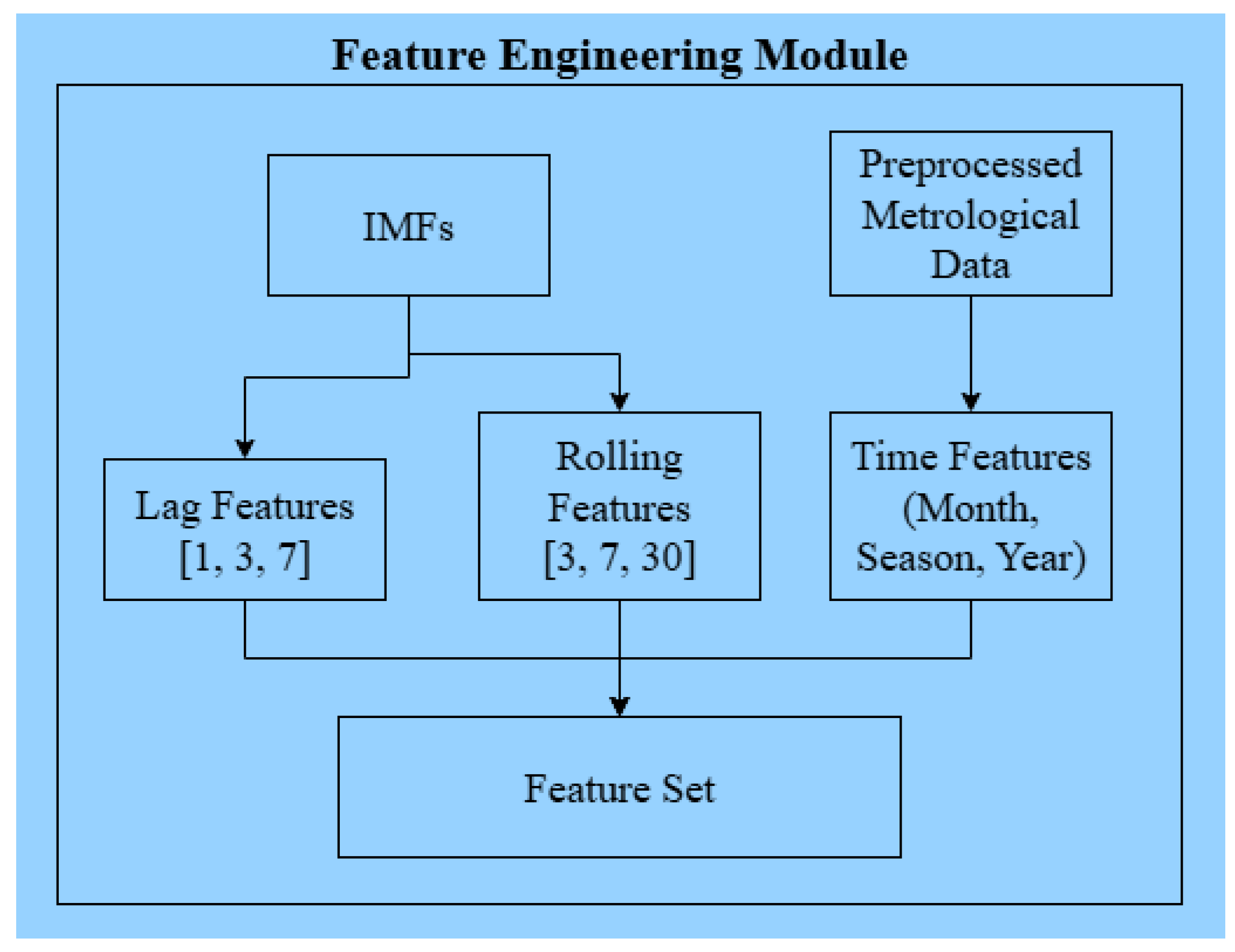
The figure shows the generation of lagged features, rolling statistical features, and time-based features from decomposed intrinsic mode functions and preprocessed meteorological data to construct the final feature set used for model training.
2.4.1. Time-Based Features
Groundwater systems exhibit pronounced seasonal and inter-annual variability influenced by monsoon cycles, evapotranspiration, and land-use changes. To represent these temporal characteristics, several time-based features were incorporated, including month, season, and year indicators. Seasonal encoding was used to distinguish between pre-monsoon, monsoon, and post-monsoon periods, allowing the model to recognize recurring recharge and depletion patterns. Long-term trend features were included to capture gradual groundwater decline associated with sustained abstraction and climate-induced changes.
2.4.2. Lagged Features
Groundwater response to climatic inputs is often delayed due to infiltration processes, subsurface storage, and aquifer characteristics. To account for these delayed effects, lagged groundwater level and quality variables were introduced as model inputs. Observations from previous time steps (e.g., one-month, three-month, and multi-season lags) were incorporated to enable the model to learn temporal dependencies and memory effects. These lagged features are particularly effective for recurrent neural networks, such as LSTM models, which are designed to capture long-term temporal relationships.
2.4.3. Rolling Statistical Features
Rolling statistical features were generated to summarize local temporal behavior and smooth short-term fluctuations. Moving averages, rolling standard deviations, and rolling minimum and maximum values were computed over multiple window sizes to highlight both short-term variability and long-term trends. These features assist the model in distinguishing persistent groundwater depletion signals from transient noise caused by isolated climatic events.
2.4.4. Climate Interaction Features
To strengthen the coupling between groundwater and climatic drivers, interaction features combining rainfall, temperature, and humidity variables were generated. These composite features help the model learn nonlinear relationships between recharge potential and atmospheric conditions, improving sensitivity to climate variability and extreme events. Such interactions are particularly important in semi-arid regions where groundwater recharge is episodic and highly dependent on rainfall intensity rather than cumulative precipitation.
2.4.5. Feature Selection and Dimensionality Control
To prevent overfitting and reduce computational complexity, feature relevance was evaluated using correlation analysis and model-based importance measures. Redundant and weakly informative features were removed, retaining only those that contributed meaningfully to prediction accuracy. This feature selection process ensured that the final input set balanced model complexity with generalization capability.
2.5. Signal Decomposition
Groundwater time series are inherently non-stationary due to the combined influence of seasonal recharge, long-term abstraction trends, and climate variability. Signal decomposition techniques provide an effective means of isolating these overlapping temporal components prior to model training. Previous studies have demonstrated that decomposition-assisted deep learning frameworks outperform standalone models in groundwater forecasting tasks [6].
In this study, Improved Complete Ensemble Empirical Mode Decomposition with Adaptive Noise (ICEEMDAN) was applied to decompose groundwater time-series data into intrinsic mode functions representing oscillations at different temporal scales. To further refine high-frequency components and suppress residual noise, Variational Mode Decomposition (VMD) was subsequently applied. This two-stage decomposition strategy is conceptually aligned with recent ensemble-based modal decomposition approaches that have shown improved robustness in groundwater level prediction using multi-data inputs [1].
Figure 6.
Signal decomposition framework for groundwater and meteorological time-series data.
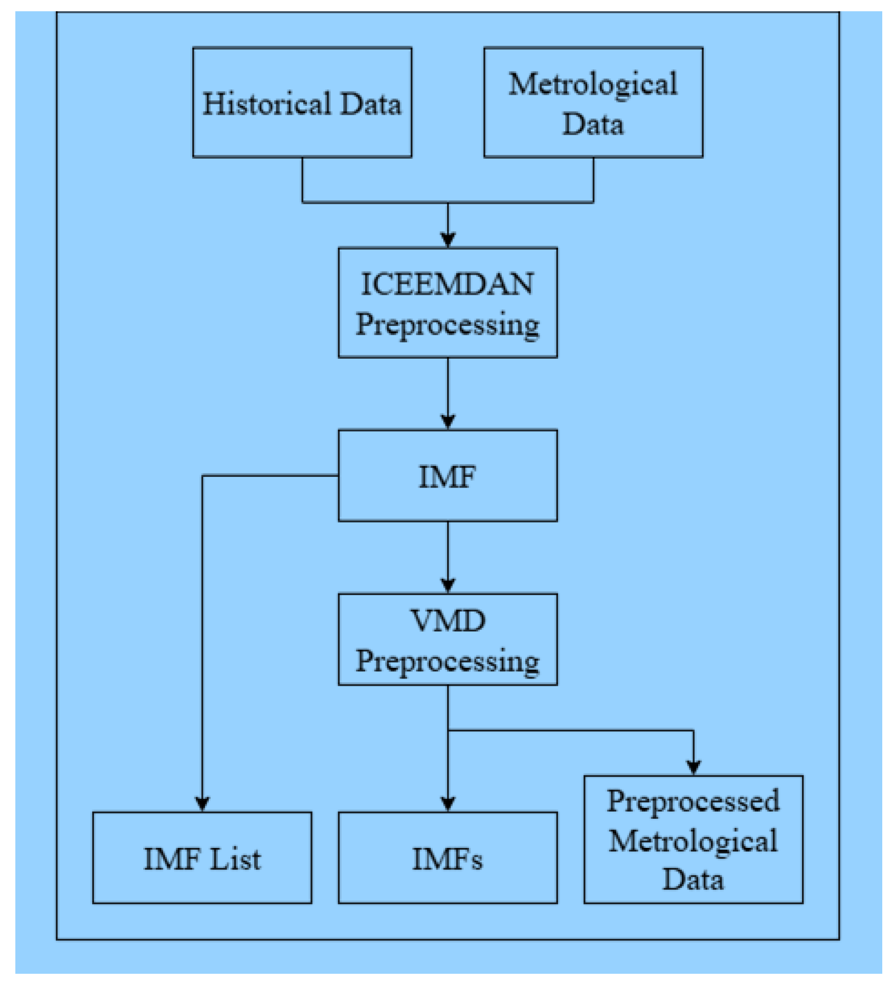
The figure illustrates the application of Improved Complete Ensemble Empirical Mode Decomposition with Adaptive Noise (ICEEMDAN) followed by Variational Mode Decomposition (VMD) to decompose historical groundwater time-series data into refined intrinsic mode functions, while meteorological variables are preprocessed to generate scale-consistent inputs for subsequent deep learning–based modeling.
2.5.1. Improved Complete Ensemble Empirical Mode Decomposition with Adaptive Noise (ICEEMDAN)
Improved Complete Ensemble Empirical Mode Decomposition with Adaptive Noise (ICEEMDAN) is an enhanced variant of empirical mode decomposition designed to overcome mode mixing and residual noise commonly observed in conventional EMD approaches. ICEEMDAN decomposes a complex time series into a finite set of Intrinsic Mode Functions (IMFs) and a residual trend component, each representing oscillations at distinct temporal scales.
In this study, ICEEMDAN was applied to groundwater level and quality time series to extract meaningful components corresponding to high-frequency fluctuations, seasonal variations, and long-term trends. By introducing adaptive noise during decomposition, ICEEMDAN ensures improved stability and consistency across ensembles, resulting in clearer separation of hydrological signals influenced by climatic and anthropogenic factors.
2.5.2. Variational Mode Decomposition
While ICEEMDAN effectively separates intrinsic components, certain high-frequency IMFs may still contain residual noise. To further refine these components, Variational Mode Decomposition (VMD) was employed as a secondary decomposition step. VMD formulates signal decomposition as a constrained variational problem, extracting modes with specific bandwidths and center frequencies.
The application of VMD to selected ICEEMDAN-derived IMFs enhances frequency resolution and suppresses spurious oscillations. This two-stage decomposition strategy improves the clarity of temporal features supplied to deep learning models, enabling more accurate learning of groundwater dynamics across multiple time scales.
2.5.3. Integration with Deep Learning Models
Each decomposed component obtained through ICEEMDAN and VMD was used as an independent input to deep learning models, particularly LSTM-based architectures. By training models on simplified and scale-specific signals rather than raw time series, the forecasting framework reduces model complexity and mitigates overfitting. The final groundwater prediction is reconstructed by aggregating outputs from individual decomposed components.
This integrated decomposition–learning approach enables the model to capture both short-term variability and long-term groundwater trends more effectively than conventional single-stage models. The decomposition process thus plays a critical role in enhancing prediction accuracy, stability, and interpretability under climate-induced non-stationary conditions.
2.6. Model Development
Advanced deep learning architectures have been increasingly adopted for groundwater level prediction due to their ability to capture complex temporal and spatial dependencies. Recent studies employing hybrid architectures, such as TCN–LSTM networks with attention mechanisms, have reported improved predictive performance compared to conventional recurrent models [4].
Building on these developments, the present study employs two complementary deep learning models: an ICEEMDAN–VMD–SMA–LSTM model optimized using a metaheuristic algorithm and a CNN–LSTM model designed to capture spatial–temporal relationships between meteorological variables and groundwater dynamics. To enhance robustness and generalization capability, an Adaptive Weighting Model ensembles the outputs of individual models, dynamically adjusting their contributions based on predictive performance.
Figure 7.
Development of the SMA–LSTM and CNN–LSTM models.
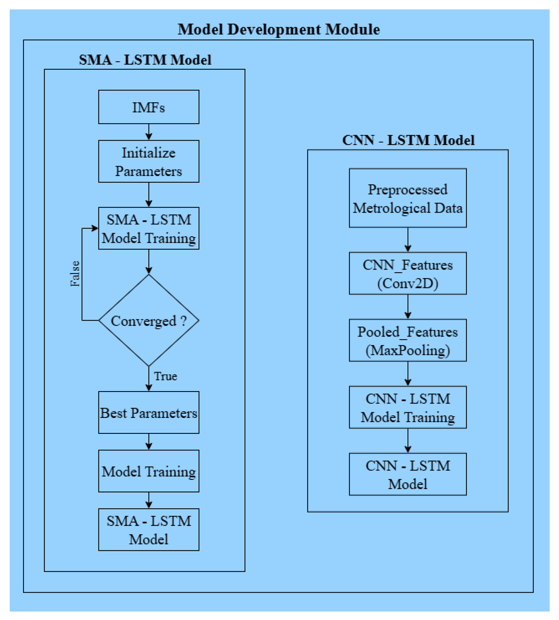
The schematic illustrates the model development process, including SMA-optimized LSTM training using decomposed intrinsic mode functions and the CNN–LSTM architecture for extracting spatial–temporal features from meteorological data.
2.6.1. Long Short-Term Memory (LSTM) Model
Long Short-Term Memory (LSTM) networks are a class of recurrent neural networks specifically designed to learn long-term dependencies in sequential data. Groundwater level and quality time series often exhibit delayed responses to recharge, extraction, and climatic drivers, making LSTM architectures particularly suitable for this application.
The LSTM model employed in this study consists of memory cells with input, forget, and output gates that regulate information flow across time steps. This gated structure enables the model to retain relevant historical information while discarding noise and irrelevant fluctuations. The LSTM model serves as a baseline temporal predictor and provides a benchmark for evaluating the effectiveness of more advanced hybrid architectures.
2.6.2. ICEEMDAN-VMD-SMA-LSTM Hybrid Model
To improve forecasting performance under non-stationary conditions, a hybrid model combining signal decomposition, deep learning, and metaheuristic optimization was developed. Following ICEEMDAN and VMD decomposition, each intrinsic component was modeled independently using LSTM networks. This approach allows the model to focus on simplified temporal patterns at different frequency scales.
Hyperparameters of the LSTM networks, including learning rate, number of hidden units, and dropout ratio, were optimized using the Slime Mould Algorithm (SMA). SMA is a population-based optimization technique inspired by the foraging behavior of slime moulds and is well-suited for navigating complex, nonlinear search spaces. The optimized configuration enhances convergence speed and predictive accuracy while reducing the risk of overfitting.
Figure 8.
Algorithmic workflow of the ICEEMDAN–VMD–SMA–LSTM model.
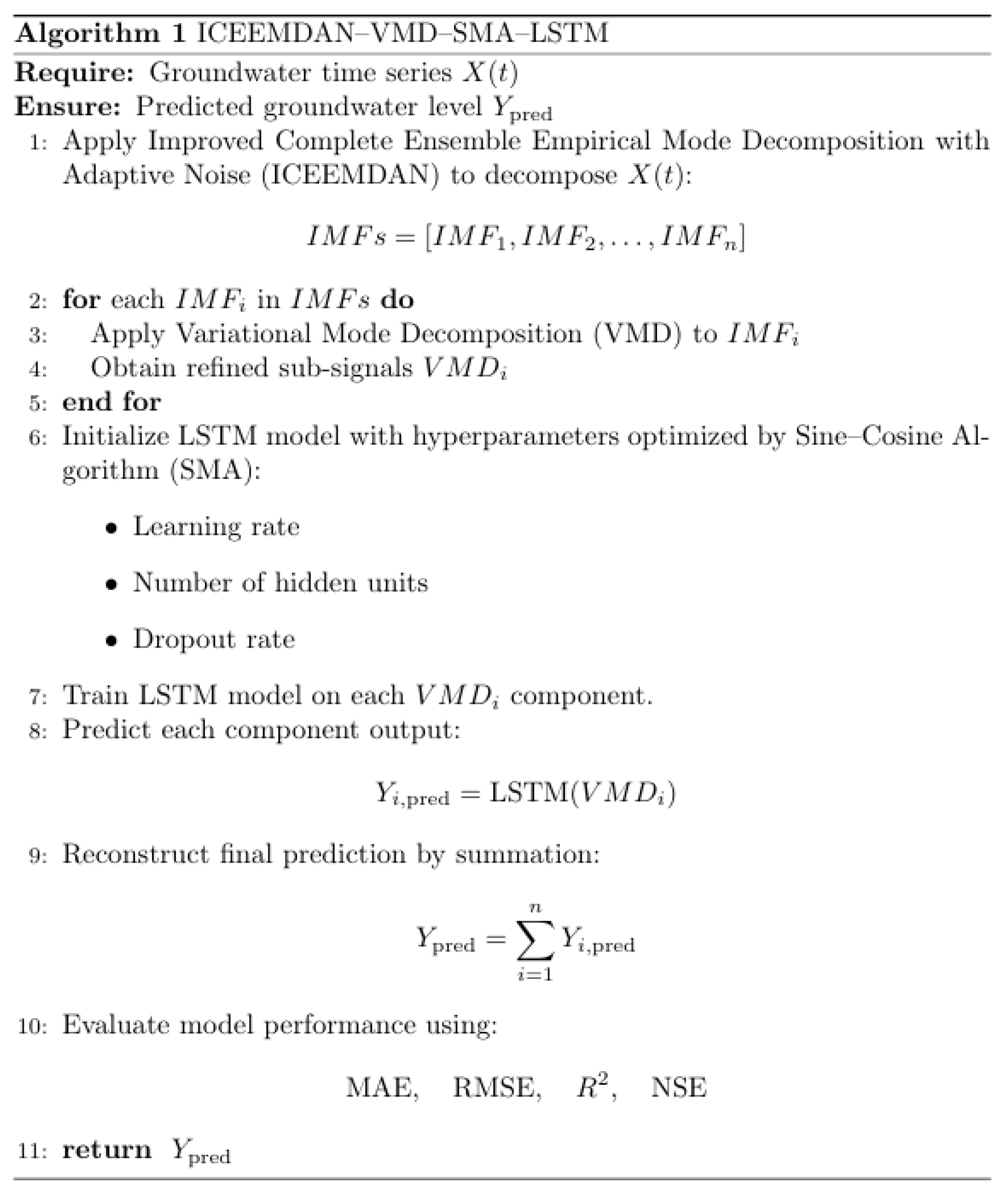
The algorithm outlines the step-by-step procedure for groundwater time-series decomposition, model training with optimized hyperparameters, component-wise prediction, reconstruction of final forecasts, and performance evaluation.
2.6.3. Convolutional Neural Network-LSTM (CNN-LSTM) Model
To incorporate spatial variability and climatic influence, a hybrid CNN–LSTM model was developed. Convolutional Neural Networks are effective in extracting spatial features from gridded meteorological data, such as rainfall and temperature distributions. In the proposed framework, CNN layers first process meteorological inputs to learn spatial patterns associated with recharge potential.
The extracted spatial features are then fed into an LSTM network to model temporal dependencies and long-term groundwater responses. This architecture enables simultaneous learning of spatial and temporal relationships, improving the model’s ability to capture regional rainfall–groundwater interactions.
2.6.4. Adaptive Weighting Model (AWM)
Given that no single model consistently outperforms others under all hydrological conditions, an Adaptive Weighting Model (AWM) was implemented to ensemble predictions from multiple base models, including LSTM, CNN–LSTM, and ICEEMDAN–VMD–SMA–LSTM. The AWM assigns dynamic weights to individual model outputs based on their recent predictive performance, subject to a convexity constraint.
Weights are updated iteratively using error-based feedback, ensuring that models with lower prediction error contribute more significantly to the final forecast. This ensemble strategy enhances robustness, reduces model bias, and improves generalization across varying climatic and hydrological regimes.
Figure 9.
Adaptive Weighting Model (AWM) for ensemble learning.
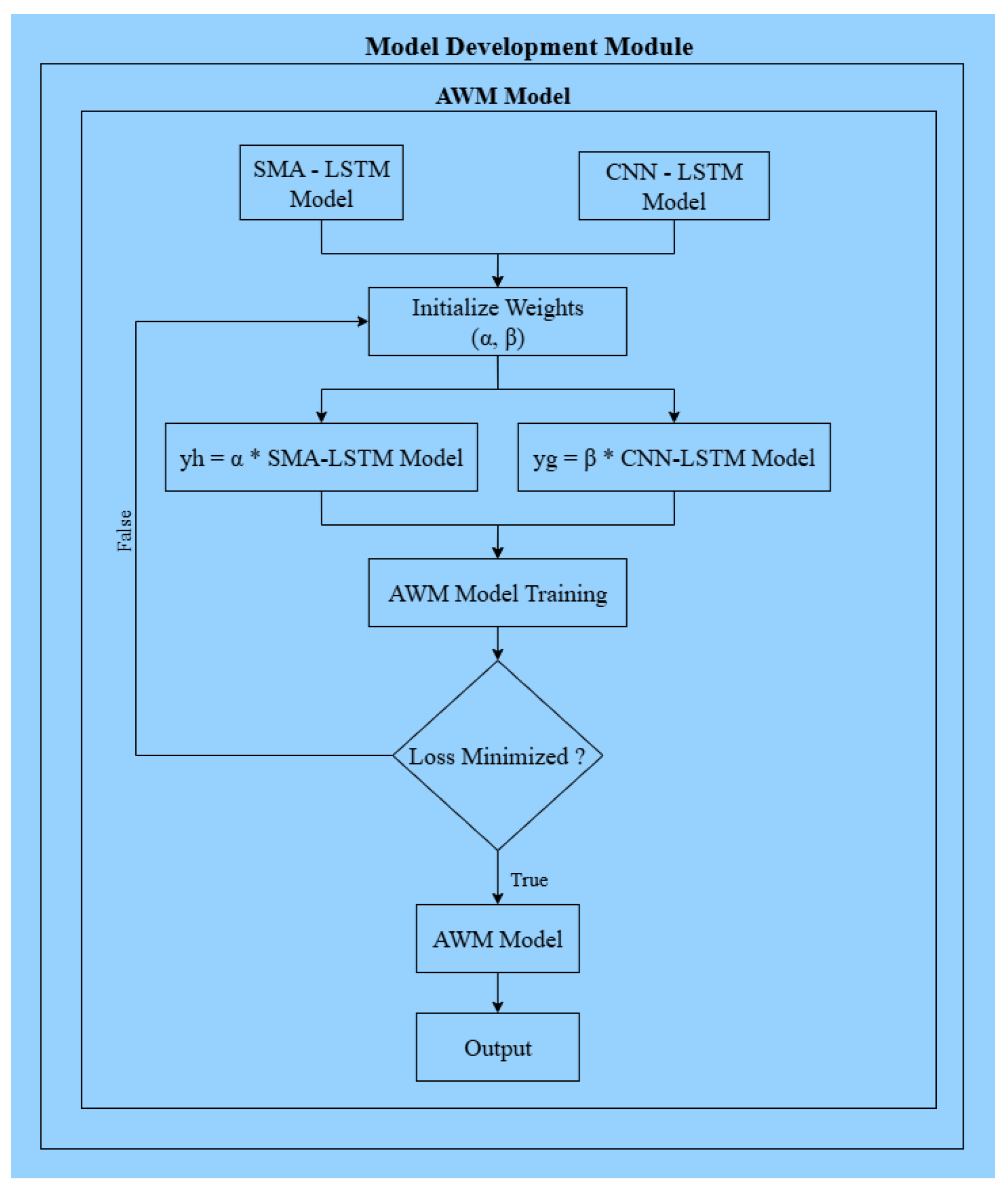
The figure depicts the ensemble framework combining SMA–LSTM and CNN–LSTM model outputs using adaptive weighting parameters to minimize prediction loss and generate the final ensemble model.
2.6.5. Model Integration and Forecast Reconstruction
The final groundwater forecast is obtained by integrating outputs from all component models through the Adaptive Weighting Model. For decomposed signals, predictions from individual intrinsic components are aggregated to reconstruct the original groundwater time series. This hierarchical integration strategy ensures that both short-term variability and long-term trends are accurately represented in the final forecast.
The hybrid model development approach adopted in this study enables effective handling of non-stationary groundwater dynamics and provides a flexible framework for incorporating additional data sources or modeling techniques in future extensions.
2.7. Model Training and Evaluation
Model training and evaluation were conducted to ensure that the proposed forecasting framework achieves high predictive accuracy, robustness, and generalization capability under varying hydrological and climatic conditions. A structured training strategy, combined with rigorous evaluation metrics, was adopted to objectively assess model performance and reliability.
2.7.1. Training-Testing Strategy
The complete dataset was divided into training and testing subsets following a chronological split to preserve the temporal structure of groundwater time series. Historical data from 1994 to 2014 were used for model training, while data from 2015 to 2024 were reserved for testing and validation. This approach prevents information leakage from future observations and ensures realistic evaluation of forecasting performance.
For deep learning models, a walk-forward (rolling-origin) validation strategy was employed during training to assess sequential prediction capability. This method allows the models to be evaluated incrementally as new observations become available, closely mimicking real-world operational forecasting scenarios.
2.7.2. Model Training Configuration
All deep learning models were trained using consistent hyperparameter settings to enable fair comparison. Training was performed using adaptive optimization algorithms, including Adam and Slime Mould Algorithm–optimized learning rates for hybrid models. Typical training parameters included batch sizes of 32, training epochs ranging from 100 to 150, and dropout regularization to mitigate overfitting.
Activation functions were selected based on model architecture, with rectified linear units used in hidden layers and linear activation in output layers. Early stopping criteria were implemented based on validation loss to prevent excessive training and improve model generalization.
2.7.3. Evaluation Metrics
Model performance was evaluated using multiple statistical metrics that collectively assess accuracy, stability, and predictive reliability. These metrics include Mean Absolute Error (MAE), Root Mean Square Error (RMSE), Coefficient of Determination (R²), and Nash–Sutcliffe Efficiency (NSE). MAE and RMSE quantify prediction error magnitude, while R² measures variance explanation and NSE evaluates hydrological model efficiency.
2.7.4. Comparative Performance Assessment
To assess the effectiveness of the proposed hybrid framework, the performance of individual models—LSTM, CNN–LSTM, and ICEEMDAN–VMD–SMA–LSTM—was compared against the ensemble Adaptive Weighting Model. All models were evaluated on identical testing datasets using uniform metrics to ensure comparability.
The ensemble model consistently outperformed standalone architectures, demonstrating lower prediction errors and higher efficiency scores. This improvement highlights the benefits of combining signal decomposition, optimized deep learning, and adaptive ensemble learning for groundwater forecasting.
2.7.5. Robustness and Generalization Analysis
Model robustness was evaluated by examining performance across different hydrological conditions, including periods of high recharge and prolonged depletion. Sensitivity to extreme climatic events was assessed to ensure stability under non-stationary conditions. The results indicate that the ensemble framework maintains consistent performance and reduces error variance compared to individual models.
Overall, the adopted training and evaluation strategy ensures that the proposed framework provides reliable and generalizable groundwater forecasts suitable for decision-support applications under climate variability.
3. Results
This section presents the quantitative results obtained from the proposed hybrid deep learning framework for groundwater level and quality forecasting in Tiruppur District. Model performance is evaluated using statistical accuracy metrics and visual analyses based on the testing dataset (2015–2024). The results focus on comparative performance across individual and ensemble models without interpretative discussion, which is addressed in the subsequent section.
3.1. Model Performance Evaluation
The predictive performance of four models—LSTM, CNN–LSTM, ICEEMDAN–VMD–SMA–LSTM, and the Adaptive Weighting Model (AWM)—was assessed using Mean Absolute Error (MAE), Root Mean Square Error (RMSE), Coefficient of Determination (R²), and Nash–Sutcliffe Efficiency (NSE). The baseline LSTM model captured general seasonal trends but exhibited higher error values under non-stationary conditions. Incorporation of spatial features through CNN–LSTM resulted in improved accuracy, while signal decomposition and metaheuristic optimization further enhanced predictive performance.
The Adaptive Weighting Model achieved the best overall performance across all evaluation metrics, indicating superior accuracy and stability when combining multiple model outputs.
Table 2 presents the quantitative comparison of groundwater forecasting models. A progressive improvement in prediction accuracy is observed from the baseline LSTM to the hybrid and ensemble-based models. The Adaptive Weighting Model achieves the lowest error values (MAE = 0.267 m, RMSE = 0.429 m) and the highest goodness-of-fit metrics (R² = 0.948, NSE = 0.938), demonstrating the effectiveness of integrating signal decomposition, optimized deep learning, and adaptive ensemble learning.
Figure 10.
Comparative evaluation of groundwater forecasting models.
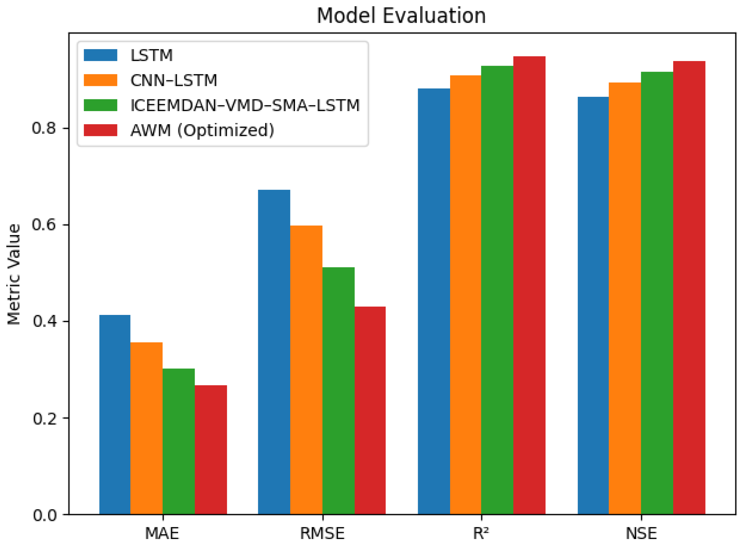
The grouped bar chart presents the performance of LSTM, CNN–LSTM, ICEEMDAN–VMD–SMA–LSTM, and the proposed Adaptive Weighting Model (AWM) based on mean absolute error (MAE), root mean square error (RMSE), coefficient of determination (R²), and Nash–Sutcliffe efficiency (NSE). The results demonstrate consistent performance improvement across successive model enhancements, with the AWM achieving the best overall accuracy.
3.2. Comparative Error Analysis
Error-based evaluation highlights the advantages of hybrid and ensemble approaches. The AWM recorded the lowest MAE (0.267 m) and lowest RMSE (0.429 m), reflecting reduced average deviation and improved handling of extreme fluctuations. Compared to the baseline LSTM model, the ensemble framework achieved approximately 35% reduction in MAE and significant improvement in RMSE, demonstrating enhanced robustness against climatic variability and groundwater non-stationarity.
The ICEEMDAN–VMD–SMA–LSTM model also showed substantial error reduction relative to standalone models, confirming the effectiveness of signal decomposition and hyperparameter optimization in isolating meaningful temporal patterns.
3.3. Goodness-of-Fit and Efficiency Metrics
Model reliability was further evaluated using R² and NSE metrics. All hybrid models achieved R² values greater than 0.90, indicating strong agreement between predicted and observed groundwater levels. The Adaptive Weighting Model achieved the highest goodness-of-fit with R² = 0.948, explaining approximately 94.8% of the observed variance in groundwater levels.
Similarly, NSE values exceeded the commonly accepted threshold of 0.75 for satisfactory hydrological model performance. The ensemble model achieved an NSE of 0.938, confirming excellent predictive efficiency and minimal deviation from observed data.
3.4. Visual Comparison of Observed and Predicted Groundwater Level
Graphical comparisons between observed and predicted groundwater levels were generated to visually assess model performance. Time-series plots indicate that the proposed models accurately replicate seasonal recharge cycles, long-term depletion trends, and short-term fluctuations. The ensemble model closely follows observed groundwater behavior during both high-recharge and low-recharge periods, with minimal lag or amplitude distortion.
Figure 11.
Comparison of observed and predicted groundwater levels.
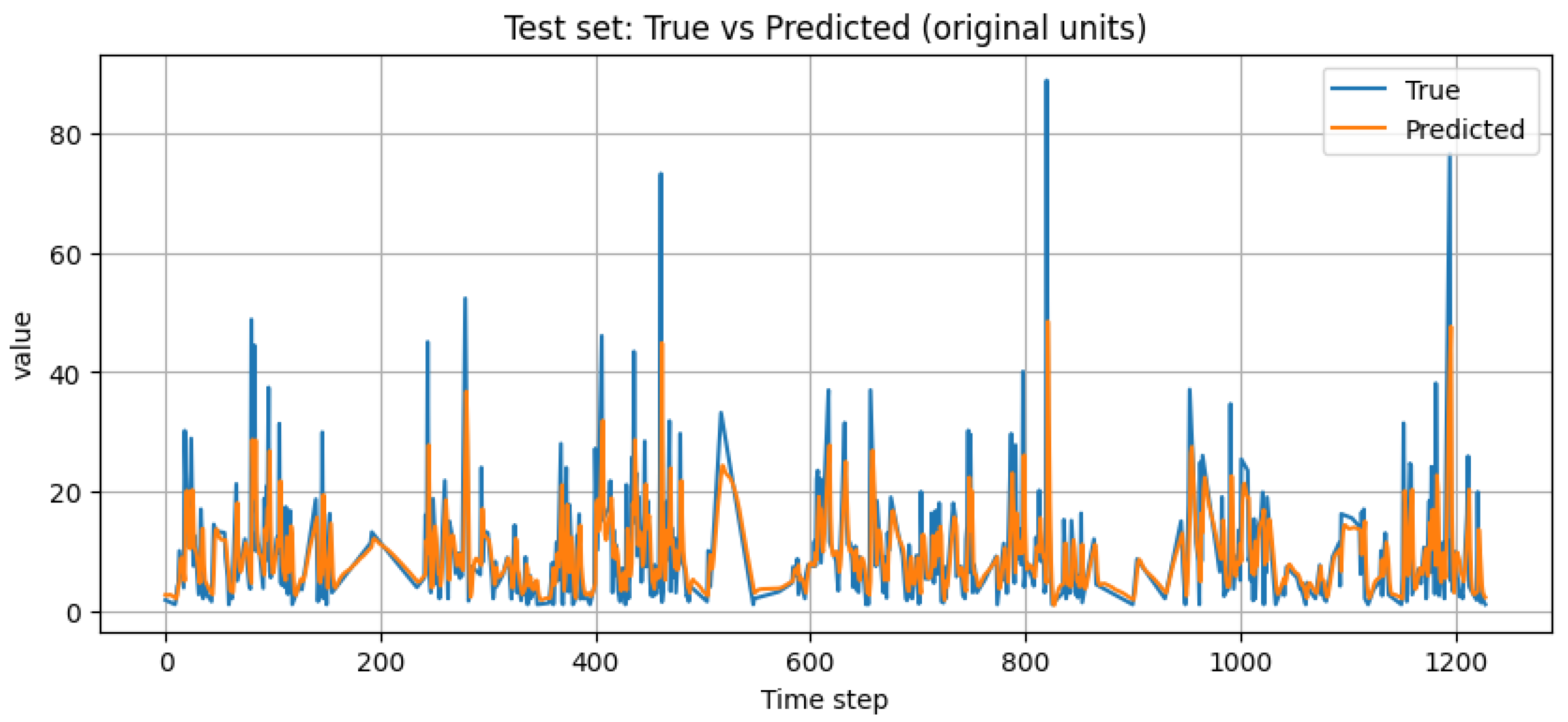
Time-series comparison between observed groundwater levels and predictions generated by the Adaptive Weighting Model for the testing period.
3.5. Correlation and Feature Interaction Analysis
Correlation analysis was performed to examine relationships among groundwater levels, meteorological variables, and groundwater quality parameters. The correlation matrix reveals strong associations between groundwater levels and rainfall, as well as moderate correlations with temperature and salinity-related quality indicators. These relationships highlight the combined influence of climatic drivers and anthropogenic stressors on groundwater dynamics.
Figure 12.
Correlation matrix of groundwater and climatic variables.
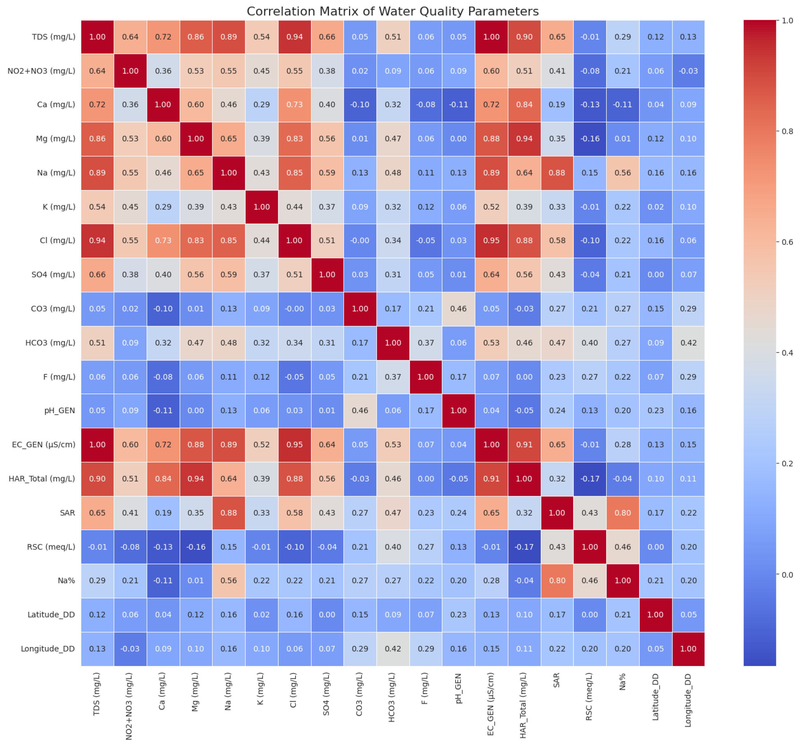
Correlation analysis showing relationships between groundwater levels, meteorological variables, and groundwater quality parameters.
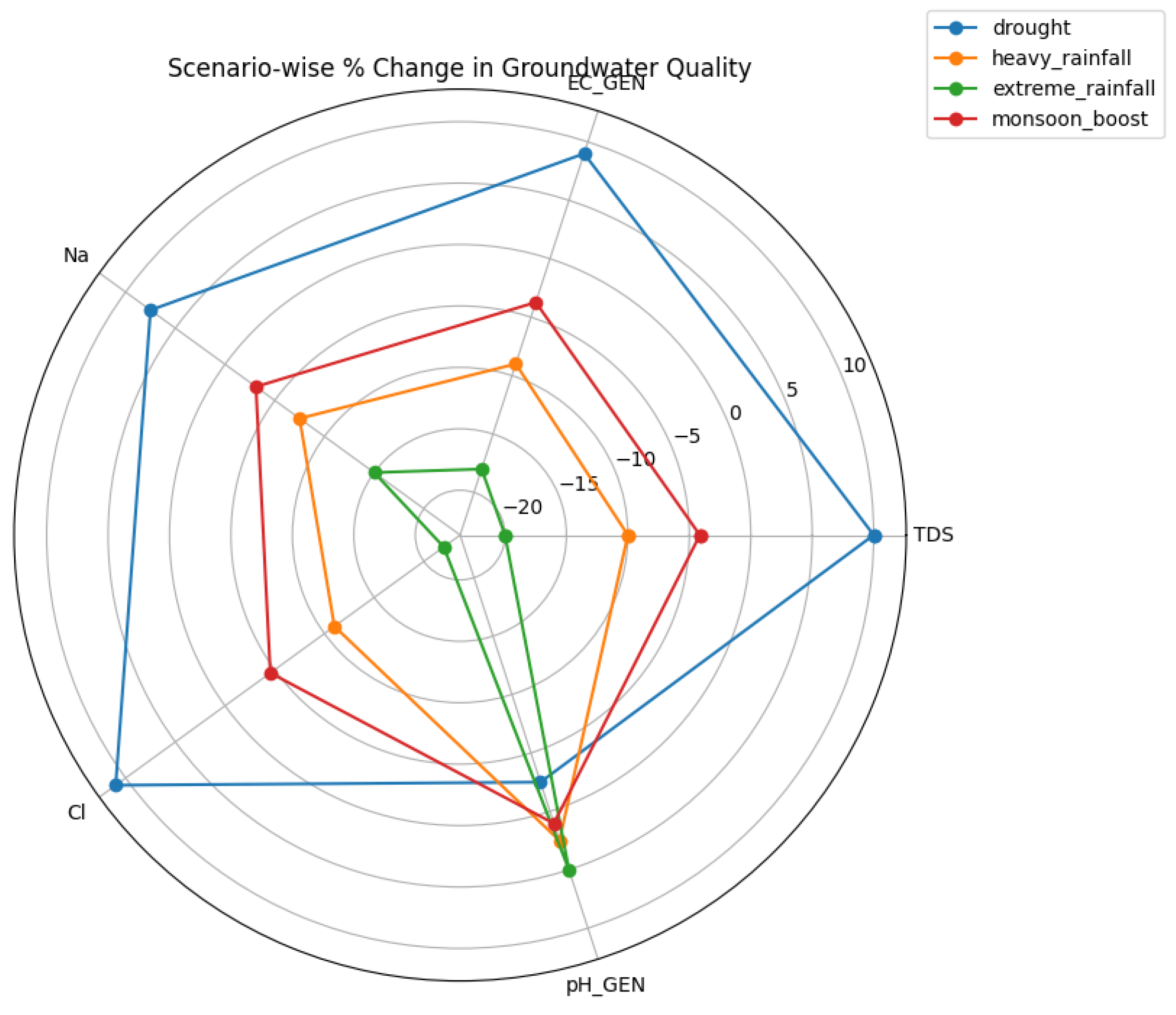
3.6. Scenario-Based Groundwater Forecasting under Climate Projections
The trained ensemble model was further applied to assess groundwater behavior under future climate scenarios derived from CMIP6 projections. Scenario-based forecasts under moderate (SSP2-4.5) and high-emission (SSP5-8.5) pathways indicate divergent groundwater trajectories. Under higher emission scenarios, projected groundwater levels exhibit accelerated decline and increased variability, reflecting heightened climatic stress.
Figure 13.
Scenario-based groundwater level projections under SSP2-4.5.
Projected groundwater level trends under the moderate-emission climate scenario using CMIP6 climate projections.
Figure 14.
Scenario-based groundwater level projections under SSP5-8.5.
Projected groundwater level trends under the high-emission climate scenario, highlighting increased variability and long-term decline.
3.7. Summary of Results
Overall, the results demonstrate that the proposed hybrid deep learning framework significantly outperforms standalone models in forecasting groundwater levels under complex, non-stationary conditions. The Adaptive Weighting Model consistently achieved the highest accuracy, stability, and efficiency across all evaluation criteria, validating the effectiveness of integrating signal decomposition, optimized deep learning, and ensemble learning for groundwater forecasting applications.
This section may be divided by subheadings. It should provide a concise and precise description of the experimental results, their interpretation, as well as the experimental conclusions that can be drawn.
4. Discussion
The results of this study demonstrate a clear and progressive improvement in groundwater forecasting accuracy with successive model enhancements. The baseline LSTM model provides reasonable predictive performance, consistent with recent comparative analyses that report moderate accuracy for conventional recurrent neural networks in groundwater level prediction tasks [7]. The incorporation of convolutional layers in the CNN–LSTM model improves performance by capturing spatial patterns in meteorological inputs, highlighting the importance of spatial–temporal learning in climate-sensitive groundwater systems.
Further improvements achieved by the ICEEMDAN–VMD–SMA–LSTM model confirm the effectiveness of decomposition-based preprocessing in handling non-stationary groundwater time series. These findings are in agreement with recent studies that report enhanced performance when modal decomposition is combined with deep learning and ensemble strategies [1,6]. The proposed Adaptive Weighting Model achieves the highest predictive accuracy and efficiency, demonstrating that ensemble learning can effectively reduce model bias and improve robustness under varying hydrological conditions.
Recent advances in transformer-based architectures have shown strong potential for long-horizon groundwater forecasting, particularly for capturing complex temporal dependencies over extended periods [8]. While such approaches were not explored in the present study, they represent a promising direction for future research.
From a management perspective, accurate and robust groundwater forecasts are essential for climate change adaptation and sustainable water resource planning. Integrating predictive models with broader surface–groundwater management frameworks has been identified as a key strategy for enhancing climate resilience and supporting informed decision-making [9]. The proposed framework provides a scalable and data-driven tool that can contribute to such integrated management efforts in groundwater-dependent regions.
4.1. Effectiveness of Signal Decomposition for Non-Stationary Groundwater Data
Groundwater time series in climate-sensitive regions often exhibit overlapping seasonal, inter-annual, and long-term trends driven by monsoon variability, extraction intensity, and land-use change. The strong performance of the ICEEMDAN–VMD–SMA–LSTM model confirms that explicit decomposition of groundwater signals prior to model training is critical for handling such complexity. ICEEMDAN effectively isolates intrinsic oscillatory components, while VMD refines high-frequency modes, resulting in cleaner inputs for deep learning models.
These findings are consistent with recent studies that report substantial error reduction when decomposition-based preprocessing is applied to groundwater forecasting models. Nazari et al. demonstrated that hybrid EMD–LSTM approaches outperform standalone LSTM models for non-stationary groundwater series, particularly in regions influenced by climate-driven trends. Similarly, Cui et al. reported improved interpretability and accuracy using secondary modal decomposition combined with deep learning ensembles. The present study extends these findings by demonstrating that a two-stage ICEEMDAN–VMD approach further enhances stability under highly variable hydroclimatic conditions.
4.2. Advantages of Hybrid Deep Learning Architectures
The improved performance of the CNN–LSTM model relative to the baseline LSTM highlights the importance of incorporating spatial meteorological information into groundwater forecasting frameworks. By extracting spatial features from climatic variables and combining them with temporal learning, the CNN–LSTM architecture effectively captures rainfall–groundwater interactions that are not adequately represented by purely temporal models.
This observation aligns with earlier work demonstrating that hybrid spatial–temporal architectures outperform single-network models in hydrological applications. Studies employing CNN–LSTM and attention-based architectures have reported enhanced predictive capability, particularly in regions where groundwater recharge is spatially heterogeneous. In the context of Tiruppur District, where rainfall distribution and recharge potential vary considerably across the landscape, spatial feature extraction plays a crucial role in improving forecast accuracy.
4.3. Ensemble Learning and Model Robustness
The Adaptive Weighting Model consistently achieved the highest predictive accuracy and efficiency, underscoring the benefits of ensemble learning for groundwater forecasting. No single model performs optimally across all hydrological regimes; however, dynamic weighting allows the ensemble framework to adaptively emphasize the most reliable predictors under changing conditions. This capability is particularly valuable under climate variability, where groundwater response mechanisms may shift over time.
The ensemble performance observed in this study is comparable to recent ensemble-based groundwater forecasting frameworks that combine multiple deep learning models with optimization strategies. Ensemble approaches have been shown to reduce model bias, mitigate overfitting, and improve generalization, especially when forecasting under extreme climatic conditions. The strong performance of the Adaptive Weighting Model confirms its effectiveness as a robust decision-support tool.
4.4. Implications for Climate-Resilient Groundwater Management
The scenario-based forecasts indicate that groundwater levels in Tiruppur District are likely to experience accelerated decline under high-emission climate scenarios. These projections emphasize the urgency of implementing adaptive groundwater management strategies, including demand regulation, managed aquifer recharge, and improved industrial water reuse practices. The proposed framework provides a data-driven tool capable of supporting such interventions by delivering timely and accurate forecasts.
From a policy perspective, the integration of real-time monitoring, climate projections, and advanced forecasting models can enhance early warning systems and inform sustainable groundwater allocation. The framework developed in this study can be readily extended to other water-stressed regions, enabling regional and national-scale groundwater resilience planning.
4.5. Limitations and Future Research Directions
While the proposed framework demonstrates strong predictive performance, certain limitations remain. Forecast accuracy depends on the quality and spatial resolution of input datasets, particularly climate projections. In addition, model transferability to regions with distinct hydrogeological characteristics may require retraining with localized data. Future research may explore the integration of transformer-based architectures, uncertainty quantification methods, and coupled surface–groundwater models to further improve long-horizon forecasting under climate change.
5. Conclusions
This study presents a hybrid deep learning framework for groundwater level and quality forecasting that integrates signal decomposition, optimized deep learning, and adaptive ensemble learning. The results demonstrate consistent performance improvement over baseline models and highlight the importance of addressing non-stationarity and climate variability in groundwater prediction. By aligning with recent advances in decomposition-based and ensemble deep learning approaches [1,6] and supporting climate-resilient groundwater management objectives [5,9], the proposed framework offers a transferable and practical solution for groundwater forecasting under changing climatic conditions.
The results demonstrate that signal decomposition using ICEEMDAN and VMD, when combined with optimized deep learning models, substantially improves forecasting accuracy compared to standalone approaches. The incorporation of spatial–temporal learning through CNN–LSTM architectures further enhanced the model’s ability to capture rainfall–groundwater interactions, while the Adaptive Weighting Model provided robust ensemble predictions across varying hydrological and climatic conditions. The ensemble framework consistently achieved high predictive performance, confirming its suitability for operational groundwater forecasting.
Scenario-based analysis using climate projections highlighted the potential for accelerated groundwater depletion under high-emission pathways, underscoring the need for proactive and climate-resilient groundwater management strategies. The proposed framework offers a scalable and data-driven decision-support tool that can support early warning systems, sustainable allocation planning, and adaptive management interventions in groundwater-dependent regions.
Overall, this research contributes to the growing body of work on AI-driven hydroclimatic forecasting by demonstrating the effectiveness of combining decomposition-based preprocessing, optimized deep learning, and ensemble learning for groundwater applications. The framework is readily transferable and can be extended to other water-stressed regions with appropriate local calibration, supporting long-term groundwater sustainability under a changing climate.
Funding
This research work is supported by Tamil Nadu Chief Minister Research Grant No. CMRG2400711.
Institutional Review Board Statement
Not applicable.
Informed Consent Statement
Not Applicable.
Data Availability Statement
The data presented in this study are available from the corresponding author upon reasonable request.
Acknowledgments
The authors acknowledge the Water Resources Department (WRD), Government of Tamil Nadu, TWAD Board, CGWB, and IMD for providing access to groundwater and meteorological datasets.
Conflicts of Interest
The authors declare no conflicts of interest.
References
- Cui, X.; Wang, Z.; Xu, N.; Wu, J.; Yao, Z. A Secondary Modal Decomposition Ensemble Deep Learning Model for Groundwater Level Prediction Using Multi-Data. Environmental Modelling & Software 2024, 175, 105969. [Google Scholar] [CrossRef]
- Li, L.; Sali, A.; Liew, J.T.; Saleh, N.L.; Ali, A.M. Machine Learning for Peatland Ground Water Level (GWL) Prediction via IoT System. IEEE Access 2024, 12, 89585–89598. [Google Scholar] [CrossRef]
- Panday, D.P.; Kumar, M.; Agarwal, V.; Torres-Martínez, J.A.; Mahlknecht, J. Corroboration of Arsenic Variation over the Indian Peninsula through Standardized Precipitation Evapotranspiration Indices and Groundwater Level Fluctuations: Water Quantity Indicators for Water Quality Prediction. The Science of the Total Environment 2024, 954, 176339. [Google Scholar] [CrossRef] [PubMed]
- Chen, X.; Yang, L.; Liao, X.; Zhao, H.; Wang, S. Groundwater Level Prediction and Earthquake Precursor Anomaly Analysis Based on TCN-LSTM-Attention Network. IEEE Access 2024, 12, 176696–176718. [Google Scholar] [CrossRef]
- Davamani, V.; John, J.E.; Poornachandhra, C.; Gopalakrishnan, B.; Arulmani, S.; Parameswari, E.; Santhosh, A.; Srinivasulu, A.; Lal, A.; Naidu, R. A Critical Review of Climate Change Impacts on Groundwater Resources: A Focus on the Current Status, Future Possibilities, and Role of Simulation Models. Atmosphere 2024, 15, 122. [Google Scholar] [CrossRef]
- Nazari, A.; Jamshidi, M.; Roozbahani, A.; Golparvar, B. Groundwater Level Forecasting Using Empirical Mode Decomposition and Wavelet-Based Long Short-Term Memory (LSTM) Neural Networks. Groundwater for Sustainable Development 2024, 28, 101397. [Google Scholar] [CrossRef]
- Saha, A.; Rahman, M.; Wu, F. Groundwater Level Prediction: Analyzing the Performance of LSTM and QLSTM Model. 2024 IEEE International Conference on Big Data (BigData) 2024, 3755–3763. [Google Scholar] [CrossRef]
- Ali, A.J.; Ahmed, A.A.; Abbod, M.F. Groundwater Level Predictions in the Thames Basin, London over Extended Horizons Using Transformers and Advanced Machine Learning Models. Journal of Cleaner Production 2024, 484, 144300. [Google Scholar] [CrossRef]
- Petpongpan, C.; Ekkawatpanit, C.; Gheewala, S.H.; Visessri, S.; Saraphirom, P.; Kositgittiwong, D.; Kazama, S. Integrated Management of Surface Water and Groundwater for Climate Change Adaptation Using Hydrological Modeling. Environment Development and Sustainability 2024, 27, 14321–14341. [Google Scholar] [CrossRef]

Table 1.
Summary of datasets used in this study.
| Dataset | Source | Time Span | Parameters |
|---|---|---|---|
| Groundwater Level | WRD, Tamil Nadu 1 | 1994 - 2024 | Depth to Water Level, Location ID, Latitude, Longitude |
| Groundwater Quality | TWAD, CGWB 2 | 2017 - 2023 | pH, EC, TDS, Ca, Mg, Na, Cl, SO₄ |
| Meteorological Data | IMD 3 | 1994 - 2024 | Rainfall, Temperature, Humidity |
| Climate Projections | CMIP6 4 | 2021 - 2040 | Precipitation, Temperature under Medium Emission (SSP2-4.5), and Very High Emission (SSP5-8.5) |
Table 2.
Model Performance Evaluation.
| Model | MAE (m) | RMSE (m) | R2 | NSE |
|---|---|---|---|---|
| LSTM | 0.412 | 0.671 | 0.881 | 0.864 |
| CNN-LSTM | 0.356 | 0.598 | 0.907 | 0.892 |
| ICEEMDAN-VMD-SMA-LSTM | 0.301 | 0.512 | 0.926 | 0.914 |
| AWM (Optimized) | 0.267 | 0.429 | 0.948 | 0.938 |
Disclaimer/Publisher’s Note: The statements, opinions and data contained in all publications are solely those of the individual author(s) and contributor(s) and not of MDPI and/or the editor(s). MDPI and/or the editor(s) disclaim responsibility for any injury to people or property resulting from any ideas, methods, instructions or products referred to in the content. |
© 2025 by the authors. Licensee MDPI, Basel, Switzerland. This article is an open access article distributed under the terms and conditions of the Creative Commons Attribution (CC BY) license (http://creativecommons.org/licenses/by/4.0/).
Copyright: This open access article is published under a Creative Commons CC BY 4.0 license, which permit the free download, distribution, and reuse, provided that the author and preprint are cited in any reuse.


