
Submitted:
20 December 2025
Posted:
22 December 2025
You are already at the latest version
Abstract
Mixed-phase clouds, in which liquid droplets and ice crystals coexist at temperatures between −38∘C and 0∘C, play a critical role in Earth’s radiation budget. In this work, we compare observations from the Advanced Very High Resolution Radiometer (AVHRR) and the Moderate Resolution Imaging Spectroradiometer (MODIS), with one global climate model, the Community Atmosphere Model version 6 – Oslo configuration (CAM6-Oslo), and three storm-resolving models: the ICOsahedral Non-hydrostatic model (ICON), the Simple Cloud-Resolving E3SM Atmosphere Model (SCREAM), and the Goddard Earth Observing System model (GEOS). Specifically, we compare mixed-phase cloud occurrence, thermodynamic partitioning, and hemispheric contrast, and introduce joint histograms of supercooled liquid fraction (SLF) and liquid effective radius (r_liq) to analyse microphysical behavior. Our results show that all models reproduce the geographic distribution of mixed-phase clouds, but differ significantly in detail. CAM6-Oslo yields the closest agreement in hemispheric SLF contrasts and SLF–r_liq relationship. Our results highlight the role of aerosol-cloud interactions and microphysics schemes in determining model performance, and demonstrate that storm-resolving models do not solve the ongoing challenge of representing mixed-phase clouds at global scales.
Keywords:
mixed-phase clouds
; aerosol-cloud interactions
; climate and storm-resolving model evaluation
1. Introduction
Mixed-phase clouds, which contain both liquid droplets and ice crystals, exert a strong influence on Earth’s radiation budget. Their radiative effect depends critically on the partitioning between liquid and ice: for the same water content, liquid clouds are optically thicker and reflect more solar radiation than ice clouds. However, the physical processes governing liquid–ice partitioning remain incompletely understood, and their representation in weather and climate models is still highly uncertain [1].
Uncertainty arises from the interplay of several factors, including temperature, vertical motion, the availability of aerosols acting as cloud condensation nuclei or ice-nucleating particles, and microphysical processes such as nucleation, riming, and secondary ice production [2,3]. These processes determine the supercooled liquid fraction (SLF), defined as the ratio of supercooled liquid water to the total condensate. Because SLF strongly affects cloud radiative forcing, evaluating how well models reproduce SLF is essential for reducing uncertainties in climate projections.
Satellite observations have provided valuable insights into mixed-phase clouds. Active sensors such as CALIPSO (Cloud-Aerosol Lidar and Infrared Pathfinder Satellite Observation) have been widely used to assess cloud phase occurrence and phase partitioning [4,5]. Passive sensors, despite their limitations, offer broader spatial and temporal coverage. Using observations from both active and passive satellite sensors, Bruno et al. (2021) [6] reported systematic hemispheric contrasts in SLF: values were generally larger in the Southern than in the Northern Hemisphere, except for continental low-level clouds where the opposite pattern was found. Whether global and storm-resolving models can reproduce these contrasts has not yet been fully assessed.
To evaluate model performance against observations, we adopt the framework introduced by Cesana et al. (2015) [7], who used joint histograms of SLF as a function of cloud top temperature (CTT). This approach provides a consistent way to compare satellite retrievals and model outputs despite differences in native variables and resolution. In this work, we extend this method by introducing joint histograms of SLF and averaged liquid effective radius (). These histograms offer additional insight into microphysical processes by linking phase partitioning with droplet size.
Building on Bruno et al. (2021) [6], the present study expands the analysis in two ways. First, we evaluate not only a global climate model—the Community Atmosphere Model version 6, Oslo configuration (CAM6-Oslo)—but also three storm-resolving models: the ICOsahedral Non-hydrostatic model (ICON), the Simple Cloud-Resolving Energy Exascale Earth System Model Atmosphere Model (SCREAM), and the Goddard Earth Observing System model (GEOS). Second, we propose the SLF– diagnostic as a new benchmark for assessing cloud microphysics.
The objectives of this study are therefore:
- To provide updated reference values for mixed-phase cloud occurrence based on satellite observations and models;
- To assess the ability of global and storm-resolving models to reproduce hemispheric contrasts of mixed-phase clouds;
- To explore the potential of SLF– relationships as a benchmark for evaluating model microphysics schemes.
2. Datasets
In this paper, datasets derived from observations, a global climate model, and three global storm-resolving models were analysed.
The observations included two passive satellite sensor-based datasets: Cloud_cci AVHRR-PMv3 (Cloud Climate Change Initiative Advanced Very High Resolution Radiometer, [8,9]), with "PM" indicating the equatorial crossing time in the afternoon; and
MODIS_D3_MODIS (Moderate Resolution Imaging Spectroradiometer (Aqua/Terra) Cloud Properties Level 3 daily [10,11]).
In Bruno et al. (2021) [6], cloud property datasets derived from the passive sensor AVHRR onboard polar-orbiting NOAA satellites were compared to the active sensor CALIOP (Cloud-Aerosol Lidar with Orthogonal Polarization) onboard the polar-orbiting CALIPSO satellite (Cloud-Aerosol Lidar and Infrared Pathfinder Satellite Observation). The AVHRR-based datasets showed a warm bias in cloud top temperature compared to CALIOP; furthermore, a thermodynamic phase mismatch was found with of liquid cloud tops in CALIOP retrieved as ice in AVHRR-based datasets. Nevertheless, AVHRR-based datasets were shown to be able to reproduce the hemispheric contrasts from the active satellite sensor CALIOP. Because of their agreement and because active sensors provide less spatial coverage than passive sensors for the same time frame, Cloud_cci v3 — the most recent AVHRR-based dataset analysed in Bruno et al. (2021) [6] — has been included in this paper (hereafter AVHRR).
MCD06COSP_D3_MODIS [10,11] is a product specifically designed to facilitate the comparison of MODIS observations and climate model output produced with the Cloud Feedback Model Intercomparison Project (CFMIP) Observation Simulator Package 2 (COSP2) simulator [12], which is included in the global climate model (GCM) dataset used in this study. The MCD06COSP_D3_MODIS dataset provides MODIS measurements from the polar-orbiting Aqua and Terra satellites, aggregated to a coarser spatial resolution ( x ) during dataset processing. The cloud optical properties are retrieved by using only one channel (3.7µm) instead of six. For brevity and readability, we hereafter refer to this dataset as MODIS.
The GCM dataset we analysed here is the atmospheric component of the Norwegian Earth System Model version 2 (NorESM2), which is based on the Community Atmosphere Model Version 6 (CAM6, [13]) and is hereafter referred to as CAM6-Oslo. CAM6-Oslo uses the OsloAero5.3 [14] aerosol scheme and aerosol-radiation-cloud interactions from [15], and is the only model in this work to treat aerosols interactively as possible cloud condensation nuclei and ice nucleating particles.We specifically used MODIS-like cloud fields from CAM6-Oslo produced by the COSP2 satellite simulator to provide the best comparison with passive satellite retrievals. This output is still referred to as CAM6-Oslo in this paper.
The three global storm-resolving model datasets we analysed are part of the DYnamics of the Atmospheric general circulation Modeled On Non-hydrostatic Domains (DYAMOND) Winter project [16]: ICON (ICOsahedral Nonhydrostatic Model, [17,18]), SCREAM (Simple Cloud-Resolving E3SM (Energy Exascale Earth System Model) Atmosphere Model, [19]), and GEOS (Goddard Earth Observing System, [20]). For consistency, the atmosphere-only experiments of all models were used in this study. As the study includes an analysis of mixed-phase clouds and the passive satellite sensors provide only cloud-top information, only the cloud top information of model outputs was used, therefore reproducing the satellite view of clouds. The following cloud parameters were considered in this study: cloud-top phase (CPH) considered either as a liquid or ice pixel (for AVHRR), or as liquid (CLW) and ice (CLI) cloud fraction (for MODIS and CAM6-Oslo), or as mass mixing ratio of ice () and liquid water (, for the DYAMOND datasets); cloud-top pressure (CTP); cloud-top temperature (CTT); cloud optical thickness (COT); and liquid cloud effective radius () at the cloud top. Not all datasets provide all variables. These are listed in Table ?? for each dataset together with the most relevant features for our study.
3. Methods
All datasets provide global data with daily or higher time resolution, here analysed near-globally (N to S), thus excluding satellite data with low confidence due to the presence of sea ice [21] and high solar zenith angle [22]. In addition to the near-global analysis, continental and marine regions were considered separately, as were different cloud types and latitudes: Northern Hemisphere mid-latitudes (NH) from N to N; Southern Hemisphere mid-latitudes (SH) from S to S. We analysed 4 years (from June 1, 2009 to May 31, 2013, see [6]) of AVHRR, MODIS, and CAM6-Oslo. The DYAMOND datasets, however, which are computationally very costly, are only available for a 30-day analysis period (January 30 - February 28, 2020) following a 10-day spin-up period. In this study, only the February portion is used.
3.1. Cloud Identification
AVHRR, MODIS and the COSP outputs from CAM6-Oslo provided the cloud top information in 2-dimensional composites as a function of latitude and longitude, while the DYAMOND datasets provided the 3-dimensional view of the atmosphere. For this reason, a top-down approach was used to locate the cloud top in the DYAMOND models. In ICON and GEOS, the cloud top was defined as the highest atmospheric layer for which kg , following [23]; to make data from SCREAM consistent with ICON and GEOS, the cloud top was defined as the highest atmospheric layer for which COT .
We also wish to account for the diurnal and COT-dependent sampling characteristics of AVHRR and MODIS when producing comparable model fields with CAM6-Oslo. Specifically, the analysis of AVHRR and MODIS was limited to daytime measurements, as the COT involved in the cloud-type classification could only be detected by satellite sensors in the visible range. To remove very thin clouds for which retrievals are more uncertain, only satellite measurements with COT > 0.3 and effective radius > 4 µm were used for this study [24]. For consistency, the same filters were applied to CAM6-Oslo, with the cloud top being defined as the highest cloud layer below an overlying COT of 0.3 for the COSP outputs.
3.2. SLF Derivation
The SLF was computed at the top of mixed-phase clouds. As in AVHRR the thermodynamic phase of a single cloudy pixel can be either liquid or ice, a reduction in spatial resolution was required to compute the SLF within gridboxes: the original latitude-longitude daily composites consisting of 3000x7200 pixels ( spatial resolution) were reorganised into 500x1200 gridboxes of 6x6 pixels ( spatial resolution), with each gridbox considered cloudy only if it contained at least two cloudy pixels (i.e., more than of the gridbox contained clouds). Furthermore, the gridboxes were only included in the analysis if the largest difference between the coldest and the warmest cloud top temperature of all valid pixels was less than C, filtering out gridboxes including clouds of very different heights (such as low- and high-level clouds, [6]). Finally, gridboxes were termed "mixed-phase" if they included coexisting liquid and ice pixels with a cloud top temperature between C and C. For each gridbox the SLF was then calculated using the number of liquid and ice pixels in the gridbox, following the Equation (1):
The model datasets and MODIS provide information on both liquid and ice content or cloud fraction in each pixel. For this reason, no gridboxes were needed to compute the SLF, as the individual pixels could already contain mixed phase. Therefore, the SLF was calculated as the ratio of the liquid cloud fraction and the sum of the liquid and ice cloud fractions (for MODIS and CAM6-Oslo, Equation (2)) or as the ratio of the mass mixing ratio of liquid water and the sum of the mass mixing ratios of ice and liquid water (for ICON, SCREAM, and GEOS, Equation (3)).
Hoose et al. (2018) [25], used a similar approach to generate cloud top liquid fraction from models and found that was C to C warmer than at SLF ∼ 0.5. This result suggests that these metrics are generally comparable, though may be slightly higher than .
ICON, SCREAM, and GEOS were analysed after coarse graining to x by averaging for better comparison with AVHRR.
3.3. Classification of Cloud Regimes and k-Means Clustering
The clustering of clouds into groups called regimes is a widely used method over the last few decades. In some works the classification is based on vertical velocity [26,27], on sea level pressure [28], or on sea surface temperature and large-scale vertical motion [29,30,31], in some others on CTP, COT, and total cloud cover [32,33,34,35,36,37,38]. Our cloud-type classification was based on standard ISCCP (International Satellite Cloud Climatology Project) cloud top pressure (CTP hPa) and cloud optical thickness (COT) thresholds, as in Bruno et al. (2021) [6]. Each COT-CTP combination was identified by the cloud name (e.g, cumulus, altocumulus, etc., [39]). As a classification of cloud types based solely on COT and CTP has limitations [40], the cloud names are mainly used as a reference to compare clouds within the same COT-CTP ranges. ICON and GEOS do not provide the COT, therefore their clouds were sorted by using CTP thresholds of hPa to classify them into high-, mid-, and low-level clouds. SCREAM provides the COT for each vertical level, therefore, the column integral of the COT for each location was considered.
As the spatial resolution of AVHRR and DYAMOND datasets has been coarsened (Section 3.2), pixel-based COT and CTP information in the original resolution has been collected in COT-CTP joint histograms. While the clouds from the MODIS and CAM6-Oslo could be directly classified on a pixel basis by using COT-CTP joint histograms, a different approach was required for AVHRR and DYAMOND datasets as COT and CTP were already collected in joint histograms. Therefore, k-means clustering was applied to the joint histograms in order to classify cloud regimes in the AVHRR and DYAMOND datasets.
The k-means algorithm [41] is a method used to sort data (points or vectors) into clusters resulting from the minimum sum of squared Euclidean distances between each cluster and its nearest cluster mean called centroid. This algorithm has limitations occurring, for example, when the distance between clusters is too large and therefore the centroids cannot move between clusters, or when stable clusters prevent the movement of centroids (e.g., high-density data regions may accumulate more centroids than necessary, with the risk of losing less dense clusters). Another difficulty with cluster analysis is finding the best number of clusters in which the data can be considered well represented. These limitations can be overcome by a better initialisation method and the iteration of the k-means with different initial solutions [42].
Initialising 42 centroids for AVHRR covered all possible COT-CTP combinations (excluding those for COT as one of the applied filters for satellite observations and simulator, the possible COT-CTP combinations were 6 times 7, from COT and CTP hPa bins, respectively) and made the k-means algorithm deterministic. In this way, the risk of neglecting some cloud types was prevented, clusters with low density were taken into account unless they were empty, and there was no need to repeat the k-means clustering since the initial centroids would be the same, and hence the final clusters too. Similarly to AVHRR, 7 prescribed initial centroids were used to cluster CTP histograms for ICON and GEOS (7 as the number of CTP bins), while 49 initial clusters (7 COT times 7 CTP combinations) were used for SCREAM, as no filters on COT has been applied to this dataset (see Section 3.1).
The final clusters needed to be merged to obtain the final 9 cloud types [39] or to organise them into 3 cloud heights. For this, the most frequent COT-CTP combination in each of the resulting clusters was used to determine to which cloud type the clusters belonged to. After this step, each of the 9 final COT-CTP joint histograms and 3 CTP histograms was individually normalised and represented a cloud type.
3.4. Geographical Distributions and Joint Histograms
Once the cloud classification was complete and the SLF computed, we derived the geographical distribution, and both the SLF-CTT and SLF- joint histograms for each cloud type.
We defined the relative frequency of occurrence of all clouds (, Equation (4)) and mixed-phase clouds (, Equation (5)) as percentage:
where the pixels are replaced by gridboxes in AVHRR.
We also defined the geographical relative frequency of occurrence of a cloud category , normalised by the number of total available observational or model output time steps (including cloud-free pixels) , for each latitude-longitude position and expressed it in percentage:
where i and j represented the position in latitude and longitude of the geographical distribution, while the cloud category is the combination of height (high, middle, or low clouds) and thermodynamic phase (all or mixed-phase clouds).
In the SLF-CTT joint histograms, the SLF changing with CTT is shown for all cloud types, with an SLF bin width of 0.05 and a CTT bin width of C. For MODIS, CTT was replaced by CTP ranging from 0 hPa to 1000 hPa with a bin width of 25 hPa. We normalised these histograms, for each cloud type, with their own total frequency of occurrence (, Equation 7, with being the absolute frequency of occurrence at bin combination (k,l), k referring to CTT or CTP, and l referring to SLF). The SLF- joint histograms show how varies with SLF in all cloud types, which we could use to interpret cloud dynamics and microphysics. We normalised these histograms individually for each cloud type (Equation 7, this time with k referring to ).
For consistency to Bruno et al. (2021) [6], we additionally normalised the histograms using an approach similar to CFADs (Contoured Frequency by Altitude Diagrams, , Equation (8)). CFAD histograms were introduced by Yuter and Houze (1995) [43] and later used in other forms for other studies (e.g., [44,45,46,47]). To highlight hemispheric contrasts in SLF over land and ocean, we computed the difference of SLF-CTT histograms using the CFAD-like histograms.
A significance test based on the p-value had been applied to these histograms, showing dots where the bins showed a statistically significant difference between NH and SH. The p-value had been computed in the highest resolution possible, i.e., for each bin and its eight surrounding bins. For this reason, no significance test could be applied to the bins at the edges of the histograms. The threshold value for significance can be arbitrary; in this work, a threshold value of 0.05 was considered [48].
4. Results
4.1. Near-Global Cloud Cover and Mixed-Phase Occurrence
The relative frequencies of occurrence of all () and mixed-phase () clouds retrieved from the datasets between North and South are summarised in Table 2.
The use of different sensors and models with individual characteristics, the application of different filters, the use of only daytime data (providing COT) in AVHRR, MODIS, and CAM6-Oslo, and the use of customised equations can lead to differences in the frequency of occurrence of clouds, so that: is more consistent between the datasets than , partly due to resolution and the definition of "mixed-phase"; of AVHRR decreases from 59.2% to 52.9% when the dataset is coarse-grained from to , as a cloudy gridbox must contain at least two cloudy pixels; ICON shows the closest (65.5%) and (6.9%) to the observations of AVHRR (52.9% and 6.2%, respectively). Figure 4-42 in the Product Validation and Intercomparison Report - ESA Cloud_cci (2020)[49] shows the time series of the monthly cloud fraction (here ) for afternoon satellite retrievals, where it can be seen that the largest monthly differences within one year are mainly confined to a 5% range (and this is always the case considering e.g., NOAA-19 only), so the large differences in between the DYAMOND datasets (including only February) and the other datasets (including full years) are not expected to depend on the different time periods analysed.
The observational datasets (AVHRR and MODIS) show large differences in both and . This may be due to the use of only the 3.7 µm channel in MODIS to retrieve cloud optical properties, as well as the combination of daily time frames of Terra and Aqua observations to provide cloud top related parameters at the final x spatial resolution. Previous validation studies including AVHRR (e.g.,[6,8]) have shown the strong performance of this dataset compared to others derived from passive and active satellite sensors. In addition, from AVHRR is closer to previous satellite studies (ranging from to for afternoon satellites; [49]) than MODIS. For these reasons, we subsequently focus on the observational data from AVHRR and using the MODIS dataset for its intended comparisons with COSP outputs from CAM6-Oslo.
4.2. Geographical Distribution and Occurrence of Clouds
Figure 1 shows the relative frequency of occurrence of all clouds derived from AVHRR and MODIS, alongside four model datasets.
Cloud types at the same height are combined to obtain high-, mid-, and low-level clouds such that ICON and GEOS, which do not provide COT, can be included in the comparison. The relative frequency of occurrence (calculated with Equation 4) refers to CTP > 680 hPa for low-level clouds, 440 hPa < CTP ≤ 680 hPa for mid-level clouds, and CTP < 440 hPa for high-level clouds, and it varies significantly between the datasets. While AVHRR and MODIS retrieve more low-level clouds (respectively, and ) than mid- ( and ) and high-level clouds ( and ), most of the models show more high-level ( ranging from to ) than low-level clouds ( ranging from to ). Despite all these differences, which may also be related to the filter applied to COT for the cloud top definition used in AVHRR, MODIS, and CAM6-Oslo, the analysed datasets mostly agree on the regions where clouds at certain heights occur. The geographical distributions in Figure 1 show that low-level clouds are mostly marine clouds while mid- and high-level clouds are found over both continents and oceans, consistent with other studies [33,35,36,50]. In particular, high- and mid-level clouds are mainly found in the extratropics and around the Intertropical Convergence Zone (ITCZ), which are areas often subject to synoptic- and mesoscale events, and low-level clouds are found mainly over the oceans, and especially over their eastern edges, where they form below a capping inversion created by the atmospheric subsidence above a low sea surface temperature.
However, the geographical distributions also show differences between the datasets: for example, low-level clouds are more widely distributed over the western sides of the oceans in AVHRR and MODIS than in the models (e.g., in the Pacific Ocean near South America), while high-level clouds are present on the eastern side of the Pacific Ocean near North America in SCREAM and GEOS, with lower frequency in AVHRR and MODIS, but these are absent in CAM6-Oslo and ICON. The differences in cloud locations between datasets, together with the differences found in , suggest a possibly wrong representation of the vertical structure of clouds in models.
Similarly to Figure 1 and Figure 2 shows the geographical distributions of the mixed-phase clouds at the three height-levels for the different datasets. The datasets show consistent patterns, with mixed-phase clouds mainly located in the mid-latitudes, in agreement with Hu et al. (2010) [51], as supercooled liquid water has been observed in both convective and stratiform clouds in these regions.
The main contributors to mixed-phase clouds are low-level clouds, except for AVHRR and CAM6-Oslo, for which mixed-phase clouds are mostly in the mid-level height, with of AVHRR in the mid-level being only 0.02% larger than in the low-level height. However, the MODIS product includes more mixed-phase clouds than the other datasets, also present in the tropics in areas where strong updrafts lead to the formation of high-level clouds with ice tops (e.g., the ITCZ). This may be due to the MODIS cloud retrieval, which averages MODIS Aqua and Terra measurements and provide cloud properties daily at spatial resolution. Therefore, some of the additional mixed-phase clouds in MODIS may be the result of averaging. The differences between the models in the geographical distributions in Figure 2 may imply different dynamics and therefore the possibility of regionally dependent cloud micro- and macrophysics within the same cloud height. Similarly to Figure 1 and Figure 2 shows different cloud locations depending on the datasets. Specific patterns in the DYAMOND models may be due to seasonal effects (e.g., boreal Winter storm track) or could suggest a possible misrepresentation of the cloud vertical structure in the models.
4.3. Temperature Dependence of Mixed-Phase Cloud Types
Figure 3 shows the SLF-CTT joint histograms of the different cloud types for AVHRR normalised as in Equation 7. Each cloud type has a unique SLF-CTT joint histogram, indicating individual cloud processes that could be driven by cloud dynamics or regional effects, e.g., different aerosol composition. Furthermore, CTT decreases from low- to mid- and high-level clouds, as expected from the direct dependence of CTT on the cloud top height, and SLF decreases with decreasing CTT. All datasets display these trends (Figures S1 to S5) although the histograms appear very different at first sight. In the temperature range between C and C, the decrease of SLF at lower temperatures could be driven by heterogeneous ice nucleation as well as secondary ice formation and the Wegener-Bergeron-Findeisen (WBF) process. For example, about 30% of all stratocumulus clouds have an SLF , while only about 10% of stratus clouds have an SLF , indicating very inefficient glaciation processes in stratus clouds compared to stratocumulus clouds or the possibility for stratus clouds to completely glaciate (very efficient glaciation processes) and quickly dissipate due to ice crystal sedimentation or snow. The presence of cirrus clouds in the mixed-phase regime may arise from the cloud-type classification based on COT–CTP thresholds [40]. Previous studies (e.g., [52]) have shown the presence of supercooled liquid droplets in cirrus clouds. However, the presence of cirrus clouds at temperatures characteristic of heterogeneous glaciation processes, as in our results, suggests the presence of lower clouds in the cirrus regime and implies that this regime represents a mixture of clouds with CTP hPa and COT .
4.4. Hemispheric Differences of Continental and Maritime Mixed-Phase Clouds
Figure 4 shows, for all datasets, the hemispheric contrast for continental and maritime areas for only cirrostratus and stratocumulus clouds, which we found to generally be the most frequent cloud types in the mixed-phase for high- and low-level clouds, respectively (Table S1). An example of derivation of these difference plots between CFAD-like histograms is shown in Figure S6 for AVHRR.
For a given CTT C in AVHRR (Figure 4, top row), cirrostratus clouds in the SH show higher SLF than in the NH over both land and the ocean, as displayed by the turquoise colors at high SLF in the difference plot. The same holds only over marine regions for stratocumulus clouds, while the opposite is true over land and at CTT C, in agreement with Bruno et al. (2021) [6]. CAM6-Oslo shows agreement with AVHRR for stratocumulus clouds over ocean but not over land, while cirrostratus clouds show inconsistent patterns in hemispheric contrasts, with higher SLF in the SH than in the NH only for SLF when considering statistically significant differences. CAM6-Oslo shows similar results to MODIS only over land for cirrostratus clouds and over both land and ocean for stratocumulus clouds (Figure 4, SLF-CTP histograms, last two rows). The DYAMOND datasets fail in representing the hemispheric differences over continental and maritime regions, with few exceptions at specific temperature ranges.
The presence of an aerosol scheme and aerosol-cloud interactions in CAM6-Oslo (see Section 2) may explain the agreement of this model with observations. However, the simulation of continental stratocumulus clouds failed to capture the hemispheric differences found in AVHRR. This suggests that the micro- and macrophysics of low-level clouds may be more influenced by the Earth’s surface than high-level clouds, making the simulation of low-level clouds more complex, especially over land where orography and aerosol type heterogeneity, distribution and transport can vary significantly in space and time. Nevertheless, CAM6-Oslo shows good agreement with MODIS in representing the hemispheric contrast of continental stratocumulus clouds. However, this is not the case for CTP hPa, where warmer temperatures can occur, reflecting the stronger disagreement with AVHRR for CTTC in the hemispheric contrast for continental stratocumulus clouds. Differences between NH and SH in cloud dynamics and cloud microphysics of the simulated cloud types, as well as the use of both day- and nighttime data and possible seasonal effects influencing results from the DYAMOND datasets (only available for February 2020) may explain the disagreements between the datasets as well as the contrast with the observations. Unfortunately, this study would not benefit from constraining the analysis to observations for February only, as the data would be insufficient due to the temporal (daily) and spatial resolution of AVHRR (coarse-grained by using gridboxes) and MODIS.
4.5. Thermodynamic Dependence of the Liquid Effective Radius in Mixed-Phase Clouds
Figure 5 shows SLF- joint histograms of the different cloud types for AVHRR (a), MODIS (b), CAM6-Oslo (c), and GEOS (d). ICON and SCREAM do not provide information on the effective radius, therefore these model datasets could not be included in the comparison. Focusing in particular on AVHRR (Figure 5a) the main results can be summarised as follows:
- Low-level and altostratus clouds are more likely to be liquid.
- In altostratus, altocumulus and high-level clouds, increases with low SLF, in agreement with Coopman et al. (2021) [53]. The presence of this trend in cirrus and cirrostratus clouds, which are expected to consist of ice crystals, may be due to a cloud misclassification [40]. In fact, it should be stressed again that the cloud type classification is based on the COT-CTP joint histograms, therefore the same cloud type may undergo different processes depending on where it forms or the atmospheric or dynamical conditions, possibly classifying some clouds in the nearby COT-CTP histogram, i.e., as a different cloud type.
- High frequency of between 12 and 13 µm is found in stratocumulus and altostratus clouds, and less but still present in cirrostratus clouds, most likely due to the a priori value assigned to , which is 12 µm [9].
Some limitations have to be considered for AVHRR. In Bruno et al. (2021) [6], a cloud-phase mismatch between AVHRR-based datasets and CALIOP (Cloud-Aerosol Lidar with Orthogonal Polarization) dataset was shown: AVHRR retrieved some clouds as ice which CALIOP retrieved as liquid. This concerned of the total collocated cloudy pixels. This implies that the liquid effective radius may be affected by errors due to incorrect phase assignment of cloudy pixels. In Stengel et al. (2017) [54] a validation study between several AVHRR datasets is presented. It shows that several datasets derived from passive satellite sensors overestimate the occurrence of liquid clouds at the expense of ice clouds. The sensitivity of passive retrievals to optically very thin ice cloud layers above liquid cloud layers is very low and the filter on COT applied in this work, which removes clouds for COT , may not be sufficient to overcome this problem. In addition, there could always be some ice in the primarily liquid pixels, and these large ice crystals may bias .
Although the histograms of MODIS (Figure 5(b)) and CAM6-Oslo (Figure 5(c)) look very different from those of AVHRR, these datasets also show an increase in with a decrease in SLF for high and mid-level clouds (CAM6-Oslo also for cumulus and stratocumulus clouds and, in general, reaching larger values than AVHRR and MODIS). This outcome is likely attributable to the propensity of cold regions, which frequently contain pristine air masses with minimal CCN, enabling the available particles to grow larger than in regions with higher CCN under equivalent humidity. GEOS (Figure 5 (d)) does not show this trend, nor the large variability in radius size shown by the other datasets.
I think the main explanation for this is that cold regions which are more likely to have low SLF are also pristine and have few CCN.
Coopman et al. (2020) [55] has shown that the glaciation of clouds with larger droplets is more likely to occur at warmer temperatures. As SLF decreases from 1 to 0 with decreasing CTT, warmer temperatures can be associated with SLF approaching 1, and this may explain why smaller values of are found as SLF approaches 1. This result can be explained by several microphysical processes: in clouds with strong updrafts, ice crystals and liquid droplets experience a decrease in temperature with height and the vapour pressure over ice and over liquid are larger than the in-cloud vapour pressure, leading to the simultaneous growth of liquid droplets and ice crystals at the expense of available water vapour [56]; during ascent in the cloud (where a decrease in SLF is expected due to the decreasing CTT), droplets can collide and aggregate, resulting in larger droplets [3]; collisions in the mixed phase temperature range can cause droplets freezing [57,58] and the formation of secondary ice [59], which can explain the decrease in SLF with the increase in . The satellite retrievals limit the size of the liquid effective radius to 35µm and 30µm in AVHRR and MODIS, respectively. This is particularly evident in Figure 5(b) for MODIS, where the size reaches values below 31µm, although the distributions in AVHRR and MODIS are centred on much lower values. In CAM6-Oslo, the distribution reaches values up to 39µm. This difference between the observational datasets and CAM6-Oslo may be due to the possible absence of mechanisms in the cloud microphysics scheme in CAM6-Oslo that should limit droplet growth, although the presence of a fixed maximum value in the observational retrievals may also lead to a bias. The decrease in with decreasing SLF in GEOS may reflect features of the model’s cloud parameterisation. In addition, the GEOS configuration for the DYAMOND Winter project simulations uses a single moment cloud microphysics scheme and the Goddard Chemistry Aerosol Radiation and Transport (GOCART) model, in which the aerosol mass of some of the key aerosol types found in the troposphere with their sources, sinks, and transport, are estimated, but the aerosol-cloud interaction is absent, with possible consequences in the simulated . In addition, CAM6-Oslo clearly shows lower in optically thicker clouds. This result may be due to the Twomey effect: clouds with a higher number concentration of liquid droplets are optically thicker and, for the same amount of water in the cloud, the droplets are smaller as they all compete for water.
4.6. Geographical Distribution of Liquid Droplets in Mixed-Phase Low-Level Clouds
Figure 6 and Figure 7 show the geographical distributions of of mixed-phase high- and low-level clouds, respectively, for AVHRR, MODIS, CAM6-Oslo, and GEOS. In both figures, continental clouds in AVHRR and MODIS generally have smaller than marine clouds, while this contrast is less pronounced in CAM6-Oslo and absent in GEOS.
Compared to the observations, CAM6-Oslo simulate larger in shallow cumulus (Figure 7) and all high-level clouds (Figure 6) and shows lower in optically thicker clouds. This result is in line with Figure 5c and possible reasons for that have been discussed in Section 4.5. GEOS underestimates and simulates very uniform distributions. This is probably related, again, to the use of a single moment microphysics scheme and the absence of aerosol-cloud interaction.
In Figure 7, the observations show larger values of also over some mountainous regions (e.g., the Andes Mountains in South America, the North American Cordillera, and the Himalayas). CAM6-Oslo shows larger values of over the Andes Mountains in South America, while GEOS shows much less variability in (Figure 7). However, the regions where larger is found can vary not only with the dataset but also with the cloud type. For example, the continental region in the SH with larger droplets in AVHRR is found in shallow cumulus clouds, while in MODIS larger droplets are found in stratus clouds. Also, the continental region in the NH with larger droplets in AVHRR includes northeastern China, while in MODIS larger droplets are found in southern Russia and part of the east coast of China. These differences may be related, again, to the averages in the MODIS retrieval, which also causes the presence of mixed-phase clouds in the tropics (as already discussed in Section 4.2). Smaller in continental than marine regions may be an indirect effect of the number concentration of aerosols acting as cloud condensation nuclei or ice-nucleating particles, being larger over land than over the ocean, so that more droplets compete for water vapour over land than over the ocean. Larger values of found over mountainous regions support the hypothesis that orographic updrafts may cause droplets to grow to larger sizes, although not all the mountainous chains show large . The continental area from to N is larger than the continental area from to S, which is mainly mountainous. If the presence of larger over land in the SH than in the NH for low-level clouds found in AVHRR and partially in MODIS is taken as true, the results in Bruno et al. (2021) [6] with AVHRR showing a lower SLF over land in the SH than in the NH for the same cloud types could be explained by the higher probability of larger droplets (likely grown by orographic updrafts) colliding and freezing at negative temperatures, as well as colliding with ice particles with the possibility to rime and produce secondary ice.
5. Conclusions
In this paper, we have used near-global ( N to S) data from passive satellite sensors (AVHRR and MODIS), three storm-resolving models from the DYAMOND project (ICON, SCREAM, and GEOS), and one global climate model (CAM6-Oslo) to analyse the cloud top thermodynamic phase, expressed in terms of supercooled liquid fraction (SLF), in relation to cloud top temperature (CTT) and mean liquid effective radius . We compared the datasets for different cloud types, classified using cloud top pressure and cloud optical thickness thresholds. The comparison included the geographical cloud cover and focused on hemispheric midlatitude ( to ) contrasts of continental and maritime regions based on 4 years analysis (from June 1, 2009 to May 31, 2013), except for the storm-resolving models, for which only February 2020 was available. To deal with the different parameters provided by the datasets for the thermodynamic phase of the cloud, we used different metrics for SLF. The main findings are summarized here:
- We derived new reference values for the fraction of mixed-phase clouds up to 60° latitude. While models exhibited a wide spread in occurrence, they generally agreed with observations on their geographical distribution, with mixed-phase clouds mainly located in the midlatitudes.
- Models showed an increase of SLF with CTT, in agreement with the observations, regardless of the cloud types and regions.
- Observations confirmed larger SLF values in the Southern Hemisphere than in the Northern Hemisphere, except for continental stratocumulus, consistent with Bruno et al. (2021) [6]. CAM6-Oslo reproduced these contrasts most closely, while the DYAMOND storm-resolving models showed only limited agreement.
- We introduced SLF– joint histograms to link phase partitioning to droplet size. Observations showed an increase in as SLF decreased. CAM6-Oslo reproduced this trend, although with a tendency to overestimate droplet size, while GEOS showed a flatter relationship and less variability.
- Geographical distributions of from observations show smaller over land than over the ocean, whereas models exhibit a less pronounced land/ocean contrast.
Several reasons may explain the disagreements found between models and observations. These include an unrealistic representation of the aerosol influence (especially for low-level clouds) in models, an insufficient representation of the cloud macro- and microphysics in models, but also uncertainties in the observational datasets (e.g., the presence of snow in mountainous regions and the use of only one channel in MODIS to retrieve the cloud optical properties may affect the quality of observations), the differences between datasets in SLF computation and the substantial differences in the satellite retrievals. We have shown that like-for-like comparisons between storm-resolving models and observations are challenging. Future high-resolution modeling experiments could employ satellite simulators or similar tools to enable fairer comparisons between models and observations. Despite these caveats, our results demonstrate that high spatial resolution alone does not guarantee a realistic representation of mixed-phase clouds (specifically, the inability of storm-resolving models to represent SLF hemispheric and land/ocean contrasts). Instead, the inclusion of interactive aerosol–cloud coupling and more advanced cloud microphysics schemes, as implemented in CAM6-Oslo, appears to be decisive. The systematic differences among models in reproducing hemispheric contrasts and SLF– relationships also have implications for simulated cloud radiative effects, since biases in phase partitioning can alter the cloud radiative effect and thus influence modeled climate feedbacks. By linking supercooled liquid fraction and droplet size, the diagnostic framework developed here provides quantitative benchmarks for evaluating and tuning cloud schemes, offering a practical path toward reducing uncertainties in the representation of mixed-phase clouds and their feedbacks in global and storm-resolving climate models.
Author Contributions
Conceptualization, O.B. and C.H.; methodology, O.B., J.S. and T.S.; software, O.B.; formal analysis, O.B..; investigation, O.B.; data curation, O.B.; writing—original draft preparation, O.B.; writing—review and editing, O.B., C.H., J.S. and T.S.; supervision, C.H.; project administration, C.H.; funding acquisition, C.H. All authors have read and agreed to the published version of the manuscript.
Funding
This project has received funding from the European Research Council (ERC) under the European Union‘s Horizon 2020 research and innovation programme under grant agreement No 714062 (ERC Starting Grant "C2Phase") and No 758005 (ERC Starting Grant “MC2”) and under the Horizon Europe research and innovation programme under grant agreement No 101045273 (ERC Consolidator Grant "STEP-CHANGE"). The projects ESiWACE and ESiWACE2 have received funding from the European Union’s Horizon 2020 research and innovation programme under grant agreements No 675191 and 823988. This work used resources of the DKRZ granted by its Scientific Steering Committee (WLA) under project IDs bk1040 and bb1153. J. K. S. was supported by a Fulbright student research grant and NASA FINESST Grant 80NSSC22K1.
Institutional Review Board Statement
Not applicable.
Data Availability Statement
For the used datasets, the following DOIs provide additional documentation and data download sites: Cloud_cci AVHRR-PMv3 — https://doi.org/10.5676/DWD/ESA_Cloud_cci/AVHRR-PM/V003; MCD06COSP_D3_MODIS — https://doi.org/10.5067/MODIS/MCD06COSP_D3_MODIS.062; CAM6-Oslo — 10.5281/zenodo.10723351. The DYAMOND model outputs supporting the conclusions of this article are archived by the German Climate Computing Centre (DKRZ) and made available through the ESiWACE project (https://www.esiwace.eu/services/dyamond)
Acknowledgments
The authors acknowledge support by the state of Baden-Württemberg through bwHPC. DYAMOND data management was provided by the Deutsches Klimarechenzentrum (DKRZ) and supported through the projects ESiWACE and ESiWACE2.
Conflicts of Interest
The authors declare no conflicts of interest.
References
- Forster, P.; Storelvmo, T.; Armour, K.; Collins, W.; Dufresne, J.L.; Frame, D.; Lunt, D.; Mauritsen, T.; Palmer, M.; Watanabe, M.; et al., The Earth’s Energy Budget, Climate Feedbacks, and Climate Sensitivity. In Climate Change 2021: The Physical Science Basis. Contribution of Working Group I to the Sixth Assessment Report of the Intergovernmental Panel on Climate Change; Masson-Delmotte, V.; Zhai, P.; Pirani, A.; Connors, S.; Péan, C.; Berger, S.; Caud, N.; Chen, Y.; Goldfarb, L.; Gomis, M.; et al., Eds.; Cambridge University Press: Cambridge, United Kingdom and New York, NY, USA, 2021; p. 923–1054. [CrossRef]
- Korolev, A.; DeMott, P.J.; Heckman, I.; Wolde, M.; Williams, E.; Smalley, D.J.; Donovan, M.F. Observation of secondary ice production in clouds at low temperatures. Atmospheric Chemistry and Physics 2022, 22, 13103–13113. [Google Scholar] [CrossRef]
- Lamb, D.; Verlinde, J. Physics and Chemistry of Clouds; 2011.
- Cesana, G.; Storelvmo, T. Improving climate projections by understanding how cloud phase affects radiation. Journal of Geophysical Research 2017, 122, 4594–4599. [Google Scholar] [CrossRef]
- Tan, I.; Storelvmo, T.; Choi, Y.S. Spaceborne lidar observations of the ice-nucleating potential of dust, polluted dust, and smoke aerosols in mixed-phase clouds. Journal of Geophysical Research 2014, 119, 6653–6665. [Google Scholar] [CrossRef]
- Bruno, O.; Hoose, C.; Storelvmo, T.; Coopman, Q.; Stengel, M. Exploring the Cloud Top Phase Partitioning in Different Cloud Types Using Active and Passive Satellite Sensors. Geophysical Research Letters 2021, 48, e2020GL089863. [Google Scholar] [CrossRef]
- Cesana, G.; Waliser, D.E.; Jiang, X.; Li, J.L.F. Multimodel evaluation of cloud phase transition using satellite and reanalysis data. Journal of Geophysical Research: Atmospheres 2015, 120, 7871–7892. [Google Scholar] [CrossRef]
- Stengel, M.; Stapelberg, S.; Sus, O.; Finkensieper, S.; Würzler, B.; Philipp, D.; Hollmann, R.; Poulsen, C.; Christensen, M.; McGarragh, G. Cloud_cci Advanced Very High Resolution Radiometer post meridiem (AVHRR-PM) dataset version 3: 35-year climatology of global cloud and radiation properties. Earth System Science Data 2020, 12, 41–60. [Google Scholar] [CrossRef]
- ATBD-CC4CLv6.2. ESA Cloud_cci Algorithm Theoretical Baseline Document v9.0 Community Cloud retrieval for Climate (CC4CL), 2023. Issue 9, Revision: 0, date of issue: 03/05/2023.
- Pincus, R.; Hubanks, P.A.; Platnick, S.; Meyer, K.; Holz, R.E.; Botambekov, D.; Wall, C.J. Updated observations of clouds by MODIS for global model assessment. Earth System Science Data 2023, 15, 2483–2497. [Google Scholar] [CrossRef]
- NASA. MCD06COSP_M3_MODIS - MODIS (Aqua/Terra) Cloud Properties Level 3 Monthly, 1x1 Degree Grid, 2022. Version 2, date of issue: 27/10/2022. [CrossRef]
- Bodas-Salcedo, A.; Webb, M.J.; Bony, S.; Chepfer, H.; Dufresne, J.L.; Klein, S.A.; Zhang, Y.; Marchand, R.; Haynes, J.M.; Pincus, R.; et al. COSP: Satellite simulation software for model assessment. Bulletin of the American Meteorological Society 2011, 92, 1023–1043. [Google Scholar] [CrossRef]
- Seland, Ø.; Bentsen, M.; Olivié, D.; Toniazzo, T.; Gjermundsen, A.; Graff, L.S.; Debernard, J.B.; Gupta, A.K.; He, Y.C.; Kirkevåg, A.; et al. Overview of the Norwegian Earth System Model (NorESM2) and key climate response of CMIP6 DECK, historical, and scenario simulations. Geoscientific Model Development 2020, 13, 6165–6200. [Google Scholar] [CrossRef]
- Kirkevåg, A.; Iversen, T.; Seland, Ø.; Hoose, C.; Kristjánsson, J.E.; Struthers, H.; Ekman, A.M.L.; Ghan, S.; Griesfeller, J.; Nilsson, E.D.; et al. Aerosol–climate interactions in the Norwegian Earth System Model – NorESM1-M. Geoscientific Model Development 2013, 6, 207–244. [Google Scholar] [CrossRef]
- Kirkevåg, A.; Grini, A.; Olivié, D.; Seland, Ø.; Alterskjær, K.; Hummel, M.; Karset, I.H.H.; Lewinschal, A.; Liu, X.; Makkonen, R.; et al. A production-tagged aerosol module for Earth system models, OsloAero5.3 – extensions and updates for CAM5.3-Oslo. Geoscientific Model Development 2018, 11, 3945–3982. [Google Scholar] [CrossRef]
- Stevens, B.; Satoh, M.; Auger, L.; Biercamp, J.; Bretherton, C.S.; Chen, X.; Düben, P.; Judt, F.; Khairoutdinov, M.; Klocke, D.; et al. DYAMOND: the DYnamics of the Atmospheric general circulation Modeled On Non-hydrostatic Domains. Progress in Earth and Planetary Science 2019, 6. [Google Scholar] [CrossRef]
- Reinert, D.; Prill, F.; Frank, H.; Denhard, M.; Baldauf, M.; Schraff, C.; Gebhardt, C.; Marsigli, C.; Zängl, G. DWD Database Reference for the Global and Regional ICON and ICON-EPS Forecasting System, 2023. Version 2.2.1, date of issue: 2023.
- Zängl, G.; Reinert, D.; Rípodas, P.; Baldauf, M. The ICON (ICOsahedral Non-hydrostatic) modelling framework of DWD and MPI-M: Description of the non-hydrostatic dynamical core. Quarterly Journal of the Royal Meteorological Society 2015, 141, 563–579. [Google Scholar] [CrossRef]
- Caldwell, P.M.; Terai, C.R.; Hillman, B.; Keen, N.D.; Bogenschutz, P.; Lin, W.; Beydoun, H.; Taylor, M.; Bertagna, L.; Bradley, A.M.; et al. Convection-Permitting Simulations With the E3SM Global Atmosphere Model. Journal of Advances in Modeling Earth Systems 2021, 13, e2021MS002544. e2021MS0025. [Google Scholar] [CrossRef]
- Putman, W.M.; Suarez, M. Cloud-system resolving simulations with the NASA Goddard Earth Observing System global atmospheric model (GEOS-5). Geophysical Research Letters 2011, 38. [Google Scholar] [CrossRef]
- King, M.D.; Platnick, S.; Yang, P.; Arnold, G.T.; Gray, M.A.; Riedi, J.C.; Ackerman, S.A.; Liou, K.N. Remote sensing of liquid water and ice cloud optical thickness and effective radius in the Arctic: Application of airborne multispectral MAS data. Journal of Atmospheric and Oceanic Technology 2004, 21, 857–875. [Google Scholar] [CrossRef]
- Grosvenor, D.P.; Wood, R. The effect of solar zenith angle on MODIS cloud optical and microphysical retrievals within marine liquid water clouds. Atmospheric Chemistry and Physics 2014, 14, 7291–7321. [Google Scholar] [CrossRef]
- Costa-Surós, M.; Sourdeval, O.; Acquistapace, C.; Baars, H.; Carbajal Henken, C.; Genz, C.; Hesemann, J.; Jimenez, C.; König, M.; Kretzschmar, J.; et al. Detection and attribution of aerosol–cloud interactions in large-domain large-eddy simulations with the ICOsahedral Non-hydrostatic model. Atmospheric Chemistry and Physics 2020, 20, 5657–5678. [Google Scholar] [CrossRef]
- Stengel, M.; Mieruch, S.; Jerg, M.; Karlsson, K.G.; Scheirer, R.; Maddux, B.; Meirink, J.; Poulsen, C.; Siddans, R.; Walther, A.; et al. The Clouds Climate Change Initiative: Assessment of state-of-the-art cloud property retrieval schemes applied to AVHRR heritage measurements. Remote Sensing of Environment 2015, 162, 363–379. [Google Scholar] [CrossRef]
- Hoose, C.; Karrer, M.; Barthlott, C. Cloud Top Phase Distributions of Simulated Deep Convective Clouds. Journal of Geophysical Research: Atmospheres 2018, 123, 10,464–10,476. [Google Scholar] [CrossRef]
- Norris, J.R.; Weaver, C.P. Improved Techniques for Evaluating GCM Cloudiness Applied to the NCAR CCM3. Journal of Climate 2001, 14, 2540–2550. [Google Scholar] [CrossRef]
- Bony, S.; Dufresne, J.L.; Le Treut, H.; Morcrette, J.J.; Senior, C. On dynamic and thermodynamic components of cloud changes. Climate Dynamics 2004, 22, 71–86. [Google Scholar] [CrossRef]
- Tselioudis, G.; Zhang, Y.; Rossow, W.B. Cloud and Radiation Variations Associated with Northern Midlatitude Low and High Sea Level Pressure Regimes. Journal of Climate 2000, 13, 312–327. [Google Scholar] [CrossRef]
- Ringer, M.A.; Allan, R.P. Evaluating climate model simulations of tropical cloud. Tellus A 2004, 56, 308–327. [Google Scholar] [CrossRef]
- Williams, K.; Ringer, M.; Senior, C. Evaluating the cloud response to climate change and current climate variability. Climate Dynamics 2003, 20, 705––721. [Google Scholar] [CrossRef]
- Williams, K.D.; Ringer, M.A.; Senior, C.A.; Webb, M.J.; McAvaney, B.J.; Andronova, N.; Bony, S.; Dufresne, J.L.; Emori, S.; Gudgel, R.; et al. Evaluation of a component of the cloud response to climate change in an intercomparison of climate models. Climate Dynamics 2006, 26, 145–165. [Google Scholar] [CrossRef]
- Jakob, C.; Tselioudis, G. Objective identification of cloud regimes in the Tropical Western Pacific. Geophysical Research Letters 2003, 30, 1–4. [Google Scholar] [CrossRef]
- Rossow, W.B.; Tselioudis, G.; Polak, A.; Jakob, C. Tropical climate described as a distribution of weather states indicated by distinct mesoscale cloud property mixtures. Geophysical Research Letters 2005, 32. [Google Scholar] [CrossRef]
- Williams, K.D.; Senior, C.A.; Slingo, A.; Mitchell, J.F.B. Towards evaluating cloud response to climate change using clustering technique identification of cloud regimes. Climate Dynamics 2005, 24, 701–719. [Google Scholar] [CrossRef]
- Williams, K.D.; Tselioudis, G. GCM intercomparison of global cloud regimes: Present-day evaluation and climate change response. Clim. Dyn. 2007, 29, 231–250. [Google Scholar] [CrossRef]
- Oreopoulos, L.; Cho, N.; Lee, D. Using MODIS cloud regimes to sort diagnostic signals of aerosol-cloud-precipitation interactions. Journal of Geophysical Research Atmospheres 2017, 122, 5416–5440. [Google Scholar] [CrossRef]
- Schuddeboom, A.; McDonald, A.J.; Morgenstern, O.; Harvey, M.; Parsons, S. Regional Regime-Based Evaluation of Present-Day General Circulation Model Cloud Simulations Using Self-Organizing Maps. Journal of Geophysical Research: Atmospheres 2018, 123, 4259–4272. [Google Scholar] [CrossRef]
- Zhang, W.; Wang, J.; Jin, D.; Oreopoulos, L.; Zhang, Z. A Deterministic Self-Organizing Map Approach and its Application on Satellite Data based Cloud Type Classification. Proceedings - 2018 IEEE International Conference on Big Data, Big Data 2018 2018, pp. 2027–2034. [CrossRef]
- Rossow, W.B.; Schiffer, R.A. Advances in Understanding Clouds from ISCCP. Bulletin of the American Meteorological Society 1999, 80, 2261–2288. [Google Scholar] [CrossRef]
- Hahn, C.J.; Rossow, W.B.; Warren, S.G. ISCCP Cloud Properties Associated with Standard Cloud Types Identified in Individual Surface Observations. Journal of Climate 2001, 14, 11–28. [Google Scholar] [CrossRef]
- Anderberg, M.R. Cluster analysis for applications; Academic Press New York, 1973; p. 359. [CrossRef]
- Fränti, P.; Sieranoja, S. How much k-means can be improved by using better initialization and repeats? Pattern Recognition 2019, 93. [Google Scholar] [CrossRef]
- Yuter, S.E.; Houze, R.A. Three-Dimensional Kinematic and Microphysical Evolution of Florida Cumulonimbus. Part II: Frequency Distributions of Vertical Velocity, Reflectivity, and Differential Reflectivity. Monthly Weather Review 1995, 123, 1941–1963. [Google Scholar] [CrossRef]
- Fu, Y.; Lin, Y.; Liu, G.; Wang, Q. Seasonal characteristics of precipitation in 1998 over East Asia as derived from TRMM PR. Advances in Atmospheric Sciences 2003, 20, 511–529. [Google Scholar] [CrossRef]
- Chen, T.; Guo, J.; Li, Z.; Zhao, C.; Liu, H.; Cribb, M.; Wang, F.; He, J. A CloudSat Perspective on the Cloud Climatology and Its Association with Aerosol Perturbations in the Vertical over Eastern China. Journal of the Atmospheric Sciences 2016, 73, 3599–3616. [Google Scholar] [CrossRef]
- Ewald, F.; Zinner, T.; Kölling, T.; Mayer, B. Remote sensing of cloud droplet radius profiles using solar reflectance from cloud sides – Part 1: Retrieval development and characterization. Atmospheric Measurement Techniques 2019, 12, 1183–1206. [Google Scholar] [CrossRef]
- Shen, C.; Li, G.; Dong, Y. Vertical Structures Associated with Orographic Precipitation during Warm Season in the Sichuan Basin and Its Surrounding Areas at Different Altitudes from 8-Year GPM DPR Observations. Remote Sensing 2022, 14, 4222. [Google Scholar] [CrossRef]
- Fisher, R. Statistical Methods for Research Workers; Biological monographs and manuals, Oliver and Boyd, 1925.
- PVIR. Product Validation and Intercomparison Report (PVIR) - ESA Cloud_cci, 2020. Issue 0, Revision: 0, date of issue: 03/02/2020.
- Tan, J.; Oreopoulos, L.; Jakob, C.; Jin, D. Evaluating rainfall errors in global climate models through cloud regimes. Climate Dynamics 2018, 50, 3301–3314. [Google Scholar] [CrossRef]
- Hu, Y.; Rodier, S.; Xu, K.m.; Sun, W.; Huang, J.; Lin, B.; Zhai, P.; Josset, D. Occurrence, liquid water content, and fraction of supercooled water clouds from combined CALIOP/IIR/MODIS measurements. Journal of Geophysical Research: Atmospheres 2010, 115. [Google Scholar] [CrossRef]
- Sassen, K. Evidence for Liquid-Phase Cirrus Cloud Formation from Volcanic Aerosols: Climatic Implications. Science 1992, 257, 516–519. [Google Scholar] [CrossRef] [PubMed]
- Coopman, Q.; Hoose, C.; Stengel, M. Analyzing the Thermodynamic Phase Partitioning of Mixed Phase Clouds Over the Southern Ocean Using Passive Satellite Observations. Geophysical Research Letters 2021, 48, e2021GL093225. [Google Scholar] [CrossRef]
- Stengel, M.; Stapelberg, S.; Sus, O.; Schlundt, C.; Poulsen, C.; Thomas, G.; Christensen, M.; Henken, C.C.; Preusker, R.; Fischer, J.; et al. Cloud property datasets retrieved from AVHRR, MODIS, AATSR and MERIS in the framework of the Cloud-cci project. Earth System Science Data 2017, 9, 881–904. [Google Scholar] [CrossRef]
- Coopman, Q.; Riedi, J.; Zeng, S.; Garrett, T.J. Space-Based Analysis of the Cloud Thermodynamic Phase Transition for Varying Microphysical and Meteorological Regimes. Geophysical Research Letters 2020, 47, e2020GL087122. [Google Scholar] [CrossRef]
- Korolev, A.V.; Mazin, I.P. Supersaturation of Water Vapor in Clouds. Journal of the Atmospheric Sciences 2003, 60, 2957–2974. [Google Scholar] [CrossRef]
- Hobbs, P.V. The Aggregation of Ice Particles in Clouds and Fogs at Low Temperatures. Journal of Atmospheric Sciences 1965, 22, 296–300. [Google Scholar] [CrossRef]
- Czys, R.R. Ice Initiation by Collision-Freezing in Warm-Based Cumuli. Journal of Applied Meteorology (1988-2005) 1989, 28.
- Korolev, A.; Leisner, T. Review of experimental studies of secondary ice production. Atmospheric Chemistry and Physics 2020, 20, 11767–11797. [Google Scholar] [CrossRef]
Figure 1.
Geographical distribution of all cloud tops for the different datasets combined at three height-levels: high- (left), mid-, and low-level (right). The relative frequency of occurrence (, Equation 4) is shown above each distribution. The colorbar indicates the geographical frequency of occurrence (Equation 6).
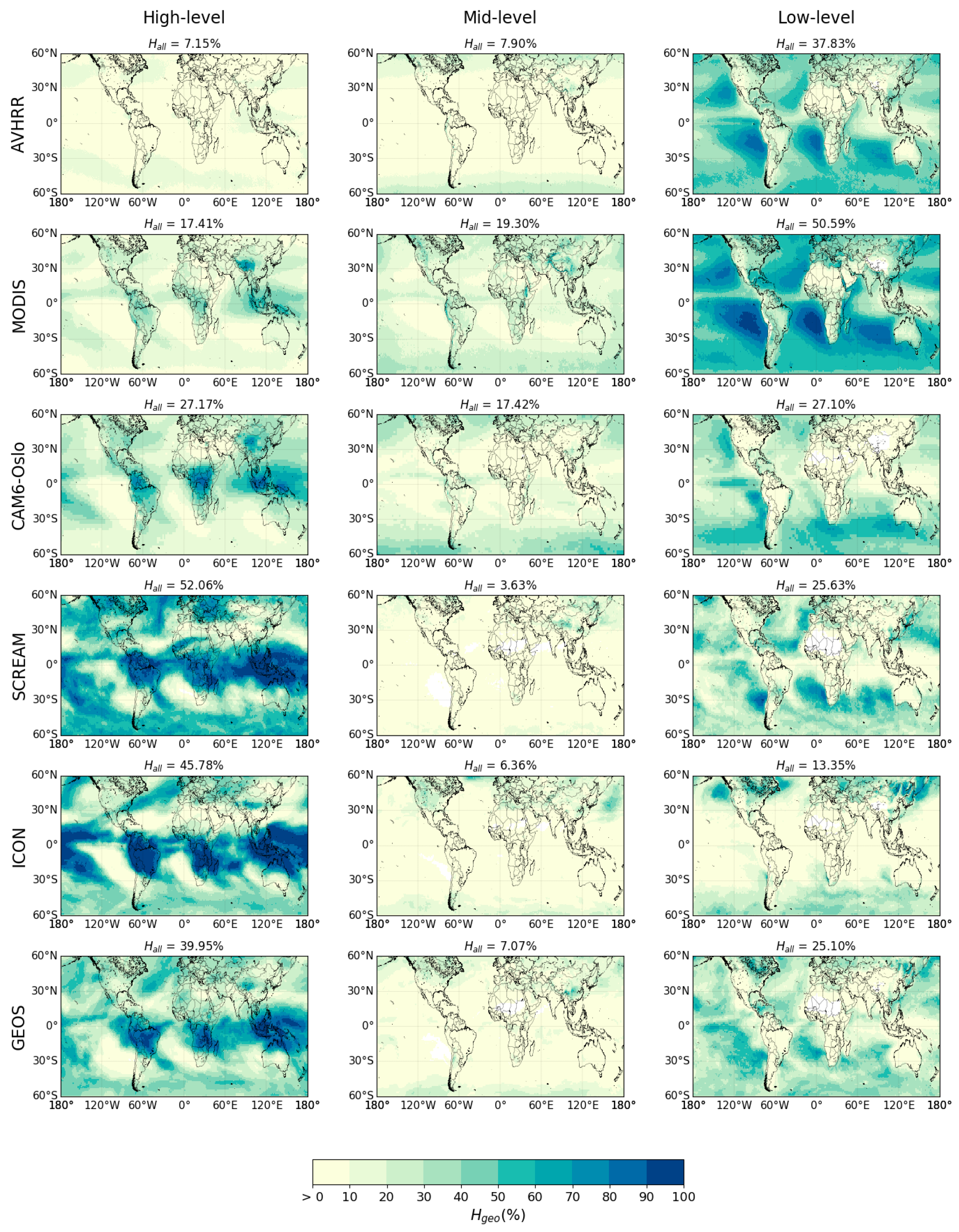
Figure 2.
Geographical distribution of mixed-phase cloud tops for the different datasets combined at three height-levels: high-(left), mid-, and low-level (right). The relative frequency of occurrence (, Equation 5) is shown above each distribution. The colorbar indicates the geographical frequency of occurrence (Equation 6). Note that the colorbar has a smaller range than in Figure 1.
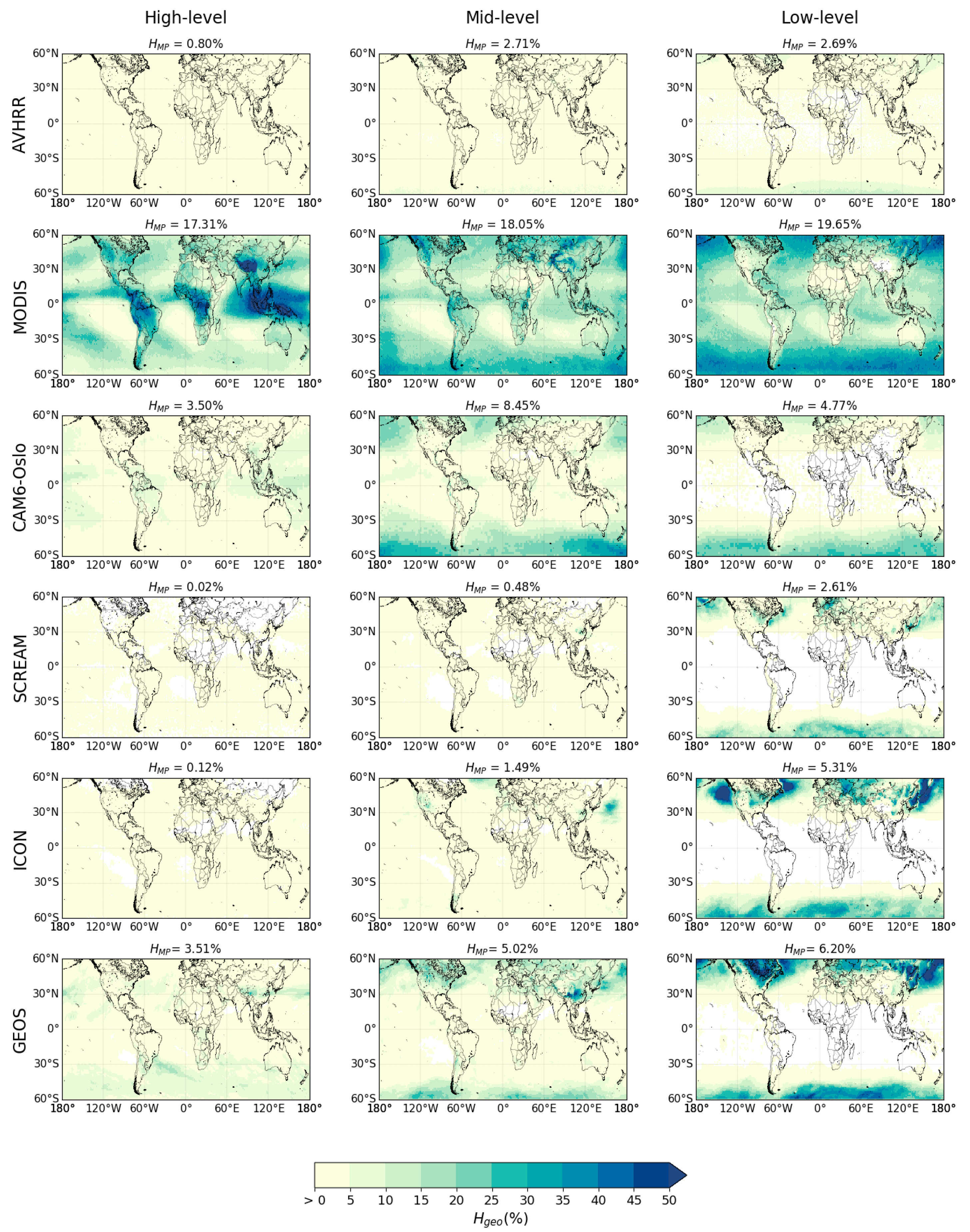
Figure 3.
SLF-CTT joint histograms of mixed-phase clouds for AVHRR. The colorbar indicates the frequency of occurrence H (Equation 7) for a given SLF-CTT bin.
Figure 3.
SLF-CTT joint histograms of mixed-phase clouds for AVHRR. The colorbar indicates the frequency of occurrence H (Equation 7) for a given SLF-CTT bin.
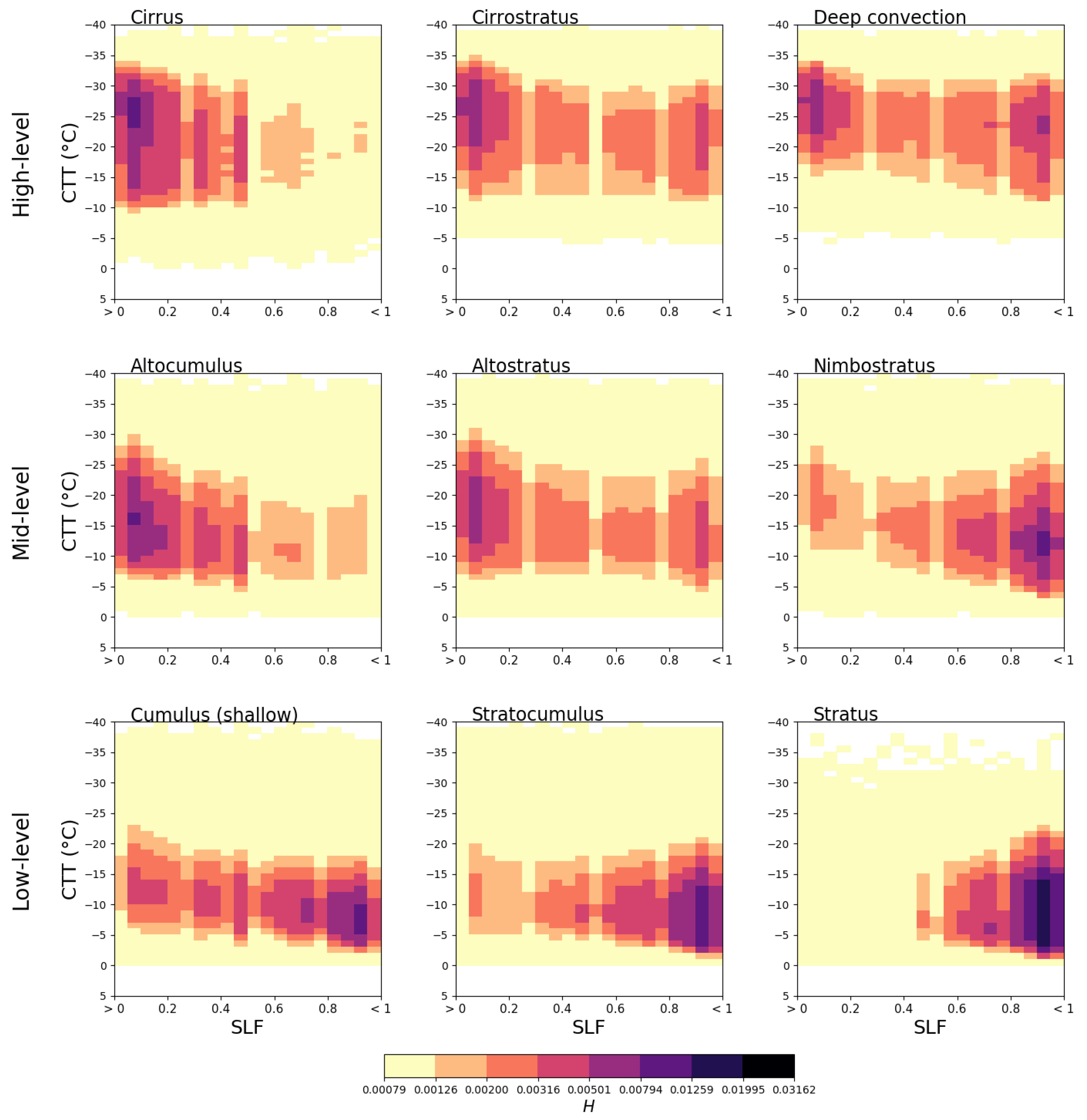
Figure 4.
Hemispheric differences (NH minus SH) between CFAD-like histograms (Equation (8)) of cirrostratus or high-level clouds (left) and of stratocumulus or low-level clouds (right) over land and the ocean for all datasets. CFAD-like histograms of MODIS are derived from SLF-CTP histograms, while both SLF-CTP and SLF-CTT histograms are used to derive CFAD-like histograms of CAM6-Oslo. Cirrostratus clouds are replaced by high-level clouds for ICON, and GEOS. The dots represent the SLF-CTT combination where the hemispheric contrast is significant with a p-value less than 0.05. The colorbar indicates the land minus ocean difference for a given SLF-CTT or SLF-CTP bin.
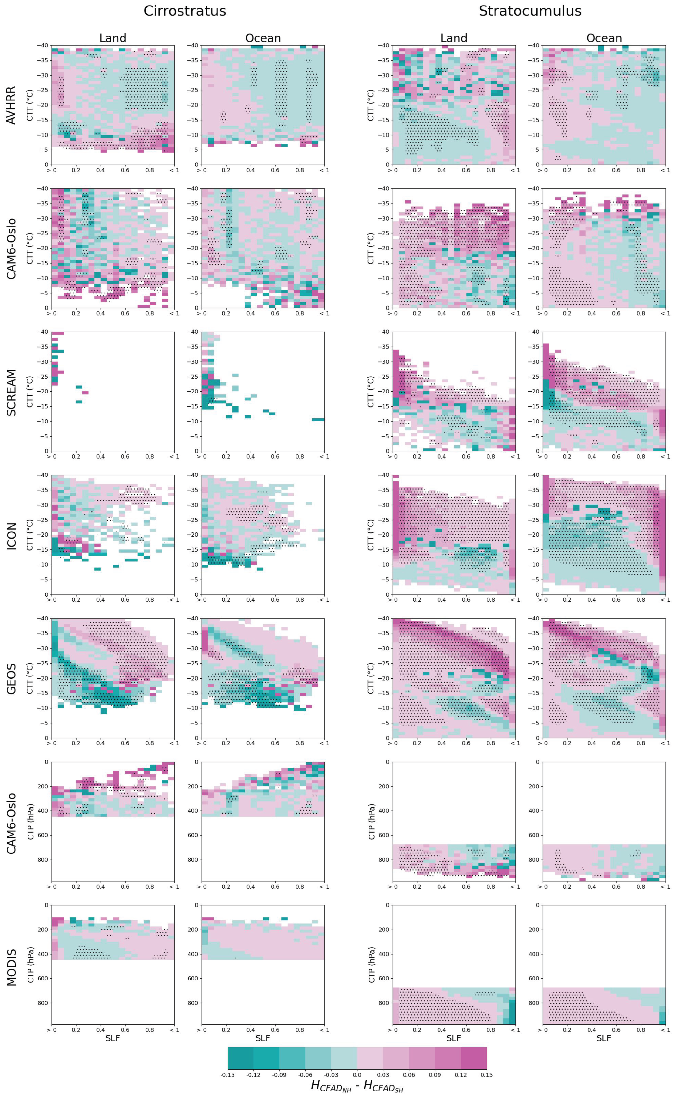
Figure 5.
SLF- joint histograms of different cloud types in the mixed phase for: (a) AVHRR, (b) MODIS, (c) CAM6-Oslo, and (d) GEOS. . The colorbar indicates the relative frequency of occurrence H (Equation 7) for a given SLF- bin.
Figure 5.
SLF- joint histograms of different cloud types in the mixed phase for: (a) AVHRR, (b) MODIS, (c) CAM6-Oslo, and (d) GEOS. . The colorbar indicates the relative frequency of occurrence H (Equation 7) for a given SLF- bin.

Figure 6.
Geographical distribution of in cirrus (left), cirrostratus (centre), and deep convective (right) clouds in the mixed phase in AVHRR, MODIS, and CAM6-Oslo, and in all high-level mixed-phase clouds in GEOS. White pixels indicate no data. Note that the colorbar is not linear.
Figure 6.
Geographical distribution of in cirrus (left), cirrostratus (centre), and deep convective (right) clouds in the mixed phase in AVHRR, MODIS, and CAM6-Oslo, and in all high-level mixed-phase clouds in GEOS. White pixels indicate no data. Note that the colorbar is not linear.
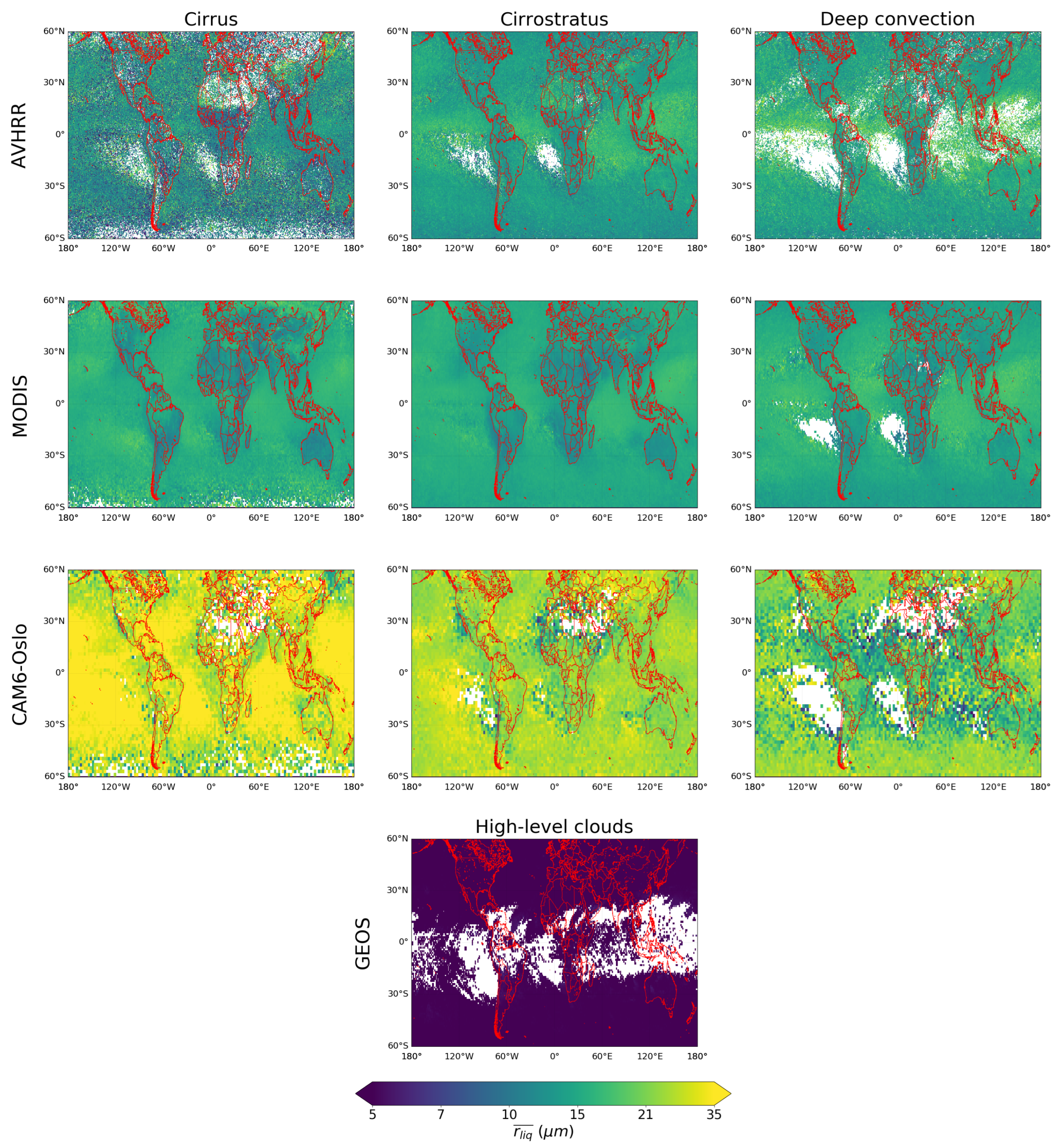
Figure 7.
Geographical distribution of in shallow cumulus (left), stratocumulus (centre), and stratus (right) clouds in the mixed phase in AVHRR, MODIS, and CAM6-Oslo, and in all low-level mixed-phase clouds in GEOS. White pixels indicate no data. Note that the colorbar is not linear.
Figure 7.
Geographical distribution of in shallow cumulus (left), stratocumulus (centre), and stratus (right) clouds in the mixed phase in AVHRR, MODIS, and CAM6-Oslo, and in all low-level mixed-phase clouds in GEOS. White pixels indicate no data. Note that the colorbar is not linear.
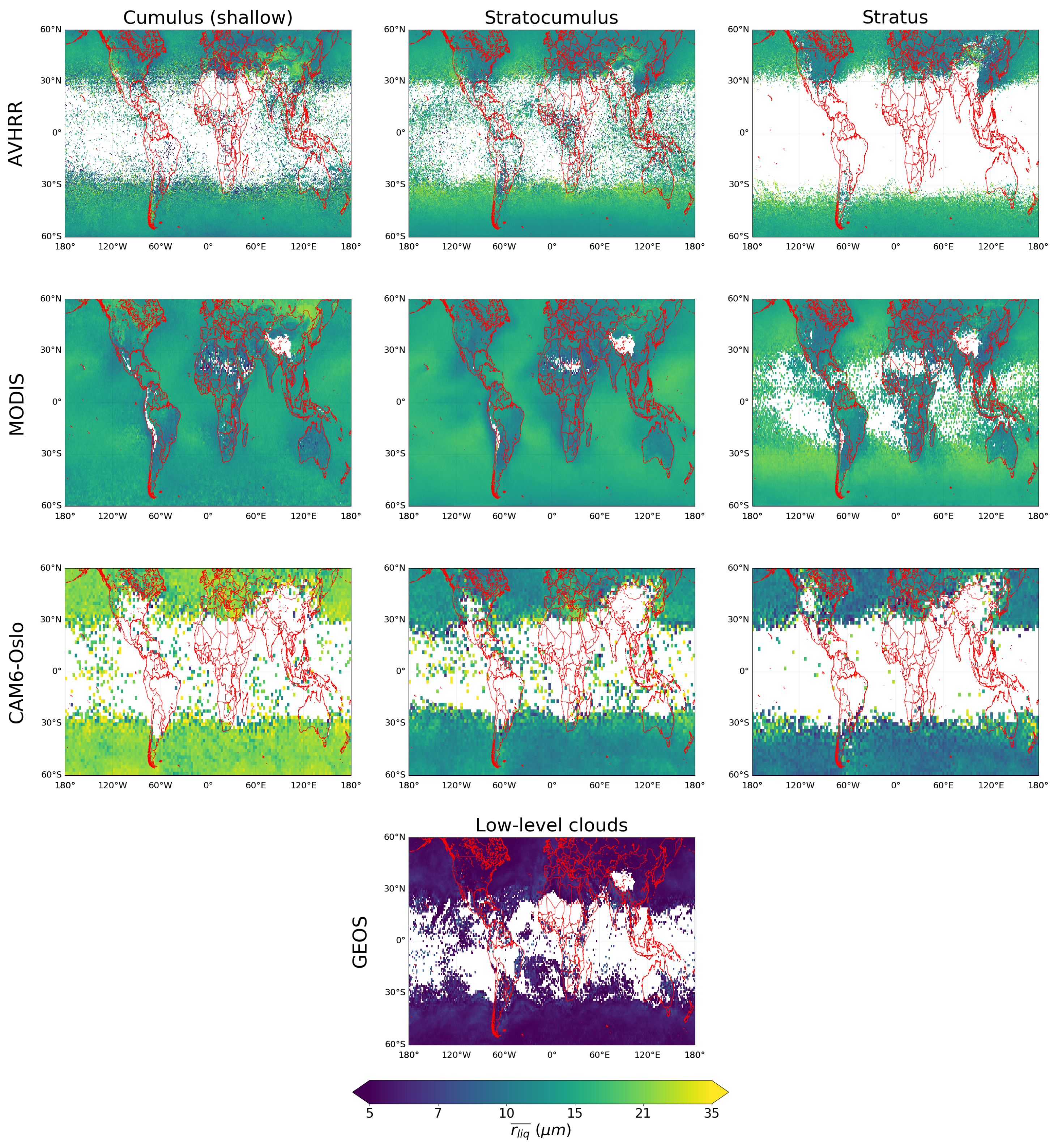

Table 2.
Relative frequency of occurrence of all ("") and mixed-phase ("") clouds, and their ratio, retrieved by all datasets included in this study between North and South, from 1 June, 2009 to 31 May 2013 for AVHRR, MODIS, and CAM6-Oslo and for February 2020 for ICON, SCREAM, and GEOS. In AVHRR, cloudy boxes and mixed-phase boxes were considered; a pixel-wise amount of "all" clouds is also provided in parenthesis.
| AVHRR | MODIS | CAM6-Oslo | SCREAM | ICON | GEOS | |
|---|---|---|---|---|---|---|
| spatial resolution | () | x | ||||
| () | ||||||
| / |
Disclaimer/Publisher’s Note: The statements, opinions and data contained in all publications are solely those of the individual author(s) and contributor(s) and not of MDPI and/or the editor(s). MDPI and/or the editor(s) disclaim responsibility for any injury to people or property resulting from any ideas, methods, instructions or products referred to in the content. |
© 2025 by the authors. Licensee MDPI, Basel, Switzerland. This article is an open access article distributed under the terms and conditions of the Creative Commons Attribution (CC BY) license (http://creativecommons.org/licenses/by/4.0/).
Copyright: This open access article is published under a Creative Commons CC BY 4.0 license, which permit the free download, distribution, and reuse, provided that the author and preprint are cited in any reuse.


