Centrality, Noncentral Selection, and the Scope of Bell–CHSH: A Measure-Theoretic Critique, Universal Inflation Bounds, Canonical Reweighting Constructions, and an Experimental Audit Protocol

1. Introduction (What Is Being Critiqued)

Bell’s theorem is a mathematically correct statement: under measurement independence (MI), local response functions, and bounded outcomes, the unconditional correlations obey CHSH$\le 2$. Modern experiments violate CHSH and therefore exclude the central local hidden-variable class provided one has controlled the relevant selection assumptions.

The critique addressed here is narrower and operational:

A CHSH violation implies nonlocality only after one has controlled/justified how the accepted sample is produced—i.e. that the accepted ensemble is not a setting-dependent hidden-variable reweighting large enough to inflate CHSH above 2.

In any real experiment, “the observed sample” is produced by hardware gates, detector thresholds, time-tag rules, coincidence identification, and analysis windows. All of these can be expressed as a setting-dependent selection weight.

A key logical separation, often blurred in informal discussion, is:

• Setting-independence of the accepted hidden ensemble: the same hidden-variable law governs accepted trials for all setting pairs. This is what lets one integrate the CHSH pointwise algebra over a single measure.
• Fair sampling / centrality relative to the hidden prior: the accepted hidden-variable law equals the underlying hidden prior, so that $E_{\mathrm{obs}}=E_{\mathrm{full}}$.

The second implies the first, but not conversely.

2. Framework

Let $S_A,S_B$ be the (finite or continuous) setting sets for Alice and Bob. Let $(\Lambda ,\mathcal{F},\rho )$ be a probability space of hidden variables $\lambda$. Measurement independence (MI) means $\rho$ does not depend on $(a,b)$.

2.1. Local Outcomes

Outcomes are bounded and local:

$$A(a,\lambda )\in [-1,1],B(b,\lambda )\in [-1,1],$$

with A depending only on $(a,\lambda )$ and B only on $(b,\lambda )$. The deterministic $\{\pm 1\}$ case is included.

2.2. Selection as a Radon–Nikodým Reweighting

Selection/detection/coincidence identification is modeled by an acceptance probability (or acceptance gate)

$$\gamma (a,b,\lambda )\in [0,1].$$

This $\gamma$ is intentionally general: it may represent independent local detections, or a joint post-processing acceptance rule (e.g. time-window coincidence assignment) that depends on both sides’ local records.

Define the acceptance rate

$$Z(a,b):=\int \gamma (a,b,\lambda )\rho \left(d\lambda \right)\in (0,1],$$

and the normalized Radon–Nikodým density

$$w(a,b,\lambda ):={\displaystyle \frac{\gamma (a,b,\lambda )}{Z(a,b)}},w(a,b,\lambda )\ge 0,\int w(a,b,\lambda )\rho \left(d\lambda \right)=1.$$

(1)

Equivalently, define the accepted-sample measure ${\nu }_{a,b}$ by

$$d{\nu }_{a,b}\left(\lambda \right)=w(a,b,\lambda )\rho \left(d\lambda \right).$$

Remark 1 

(Local-factorized detection as a special case). If selection is generated by independent local detection probabilities ${\eta }_A(a,\lambda ),{\eta }_B(b,\lambda )\in [0,1]$ with acceptance iff both sides detect, then one has

$$\gamma (a,b,\lambda )={\eta }_A(a,\lambda ){\eta }_B(b,\lambda ),$$

which is the usual “detection loophole” structure. None of the bounds below require factorization; only (1) is used.

2.3. Observed vs. Unconditional Correlations

Define the observed (accepted-sample) correlation

$$E_{\mathrm{obs}}(a,b):=\int A(a,\lambda )B(b,\lambda )d{\nu }_{a,b}\left(\lambda \right)=\int A(a,\lambda )B(b,\lambda )w(a,b,\lambda )\rho \left(d\lambda \right),$$

and the unconditional (“full”) correlation

$$E_{\mathrm{full}}(a,b):=\int A(a,\lambda )B(b,\lambda )\rho \left(d\lambda \right).$$

For a CHSH quartet $(a,a^{\prime },b,b^{\prime })$, define

$$S_{\mathrm{obs}}:=|E_{\mathrm{obs}}(a,b)-E_{\mathrm{obs}}(a,b^{\prime })|+|E_{\mathrm{obs}}(a^{\prime },b)+E_{\mathrm{obs}}(a^{\prime },b^{\prime })|.$$

Also define the unconditional CHSH expression

$$S_{\mathrm{full}}:=|E_{\mathrm{full}}(a,b)-E_{\mathrm{full}}(a,b^{\prime })|+|E_{\mathrm{full}}(a^{\prime },b)+E_{\mathrm{full}}(a^{\prime },b^{\prime })|.$$

2.4. A Quantitative Noncentrality Statistic

Define the $L^1$ deviation from centrality

$$\delta (a,b):=\int |w(a,b,\lambda )-1|\rho \left(d\lambda \right),\delta :=\underset{a,b}{sup}\delta (a,b).$$

(2)

Note that $\mathrm{TV}({\nu }_{a,b},\rho )=\frac{1}{2}\delta (a,b)$ and $\delta (a,b)\in [0,2]$.

3. Where Bell–CHSH Actually Lives: Unconditional and Setting-Independent Sectors

3.1. The Pointwise CHSH Algebra

Lemma 1 

(Pointwise CHSH bound). Fix λ. For any $a,a^{\prime },b,b^{\prime }$ and any $A,B\in [-1,1]$,

$$|A(a,\lambda )B(b,\lambda )-A(a,\lambda )B(b^{\prime },\lambda )|+|A(a^{\prime },\lambda )B(b,\lambda )+A(a^{\prime },\lambda )B(b^{\prime },\lambda )|\le 2.$$

Proof. 

This is the standard CHSH algebra; boundedness $\left|A\right|,\left|B\right|\le 1$ is enough. (Determinism is not required.) □

3.2. Unconditional Bell–CHSH (The Theorem Proper)

Theorem 1 

(Unconditional Bell–CHSH). Assume MI, locality, and bounded outcomes. Then for any quartet $(a,a^{\prime },b,b^{\prime })$,

$$S_{\mathrm{full}}\le 2.$$

Proof. 

Lemma 1 holds pointwise in $\lambda$. Integrate w.r.t. $\rho$. □

3.3. Setting-Independent Selection (Enough to Apply CHSH to the Accepted Sample)

Definition 1 

(Setting-independent selection). Selection issetting-independentif there exists a probability measure ν on Λ such that ${\nu }_{a,b}=\nu$ for all $(a,b)$. Equivalently, $w(a,b,\lambda )=w\left(\lambda \right)$ ρ-a.e. (no setting dependence in the RN density).

Theorem 2 

(CHSH on the accepted sample under setting-independent selection). Assume MI, locality, bounded outcomes, and setting-independent selection (Definition 1). Then for any quartet $(a,a^{\prime },b,b^{\prime })$,

$$S_{\mathrm{obs}}\le 2.$$

Proof. 

Under setting-independent selection, each $E_{\mathrm{obs}}(a,b)$ is an integral of $A(a,\lambda )B(b,\lambda )$ with respect to the same measure $\nu$. Apply Lemma 1 pointwise and integrate w.r.t. $\nu$. □

Remark 2 (What setting-independence doesnotgive)Setting-independent selection doesnotimply that the accepted ensemble equals the full ensemble: one can have $\nu \ne \rho$ (hence $\delta >0$) while still having $S_{\mathrm{obs}}\le 2$. What breaks CHSH on accepted data issetting dependenceof ${\nu }_{a,b}$, not merely $\nu \ne \rho$.

3.4. Fair Sampling/Centrality (Accepted Ensemble Equals the Hidden Prior)

Definition 2 

(Coincidence centrality / fair sampling). Selection iscentral(fair sampling) if

$${\nu }_{a,b}=\rho \mathrm{for}\mathrm{all}(a,b).$$

Equivalently, $w(a,b,\lambda )=1$ρ-a.e. for all $(a,b)$, or $\delta =0$.

Lemma 2 

(A sufficient “strong” condition). If $\gamma (a,b,\lambda )$ factorizes as $\gamma (a,b,\lambda )={\eta }_A\left(a\right){\eta }_B\left(b\right)$ with no λ-dependence, then selection is central in the sense of Definition 2.

Proof. 

If $\gamma (a,b,\lambda )={\eta }_A\left(a\right){\eta }_B\left(b\right)$ then $Z(a,b)={\eta }_A\left(a\right){\eta }_B\left(b\right)\int 1d\rho ={\eta }_A\left(a\right){\eta }_B\left(b\right)$ and hence $w=\gamma /Z\equiv 1$. □

Remark 3 (Centrality doesnotimply $\lambda$-independent local efficiencies)The converse of Lemma 2 is false: $w\equiv 1$ (centrality at the accepted-ensemble level) only forces $\gamma (a,b,\lambda )$ to be λ-independent for eachpair$(a,b)$; it does not force any particular factorization, nor λ-independence of individual local detection probabilities in a factorized model.

Theorem 3 

(Centrality identity). Assume MI, locality, bounded outcomes, and central selection (Definition 2). Then

$$E_{\mathrm{obs}}(a,b)=E_{\mathrm{full}}(a,b)\mathrm{for}\mathrm{all}(a,b),$$

and hence for any quartet $S_{\mathrm{obs}}\le 2$.

Proof. 

If $w\equiv 1$ then $E_{\mathrm{obs}}=E_{\mathrm{full}}$ by definition. Then $S_{\mathrm{obs}}=S_{\mathrm{full}}\le 2$ by Theorem 1. □

Remark 4 (Hiddenness is irrelevant to thealgebra, but selection is not)Lemma 1 is pointwise in λ. Whether λ is observed or not does not affect CHSH. What matters is whether the four accepted-sample expectations are taken with respect to asinglemeasure (setting-independent selection) or a setting-dependent family ${\nu }_{a,b}$ (noncentral selection).

4. Noncentral Selection: Universal Deviation and CHSH Inflation Bounds

4.1. Deviation of a Single Correlation

Theorem 4 

(Deviation bound). For each $(a,b)$,

$$|E_{\mathrm{obs}}(a,b)-E_{\mathrm{full}}(a,b)|\le \delta (a,b).$$

Equivalently,

$$|E_{\mathrm{obs}}(a,b)-E_{\mathrm{full}}(a,b)|\le 2\mathrm{TV}({\nu }_{a,b},\rho ).$$

Proof. 

$$E_{\mathrm{obs}}-E_{\mathrm{full}}=\int A(a,\lambda )B(b,\lambda )(w-1)d\rho ,$$

so by $\left|AB\right|\le 1$,

$$|E_{\mathrm{obs}}-E_{\mathrm{full}}|\le \int |w-1|d\rho =\delta (a,b).$$

 □

4.2. CHSH Inflation

Theorem 5 

(CHSH inflation bound). Assume MI, locality, and bounded outcomes. For any quartet $(a,a^{\prime },b,b^{\prime })$,

$$S_{\mathrm{obs}}\le 2+\delta (a,b)+\delta (a,b^{\prime })+\delta (a^{\prime },b)+\delta (a^{\prime },b^{\prime }).$$

In particular,

$$S_{\mathrm{obs}}\le min\{4,2+4\delta \}.$$

Equivalently,

$$S_{\mathrm{obs}}\le min\left\{4,2+8\underset{a,b}{sup}\mathrm{TV}({\nu }_{a,b},\rho )\right\}.$$

Proof. 

Apply Theorem 4 to each of the four setting pairs in $S_{\mathrm{obs}}$ and use the triangle inequality inside each absolute value. One obtains

$$S_{\mathrm{obs}}\le S_{\mathrm{full}}+\delta (a,b)+\delta (a,b^{\prime })+\delta (a^{\prime },b)+\delta (a^{\prime },b^{\prime }).$$

Then apply Theorem 1 to bound $S_{\mathrm{full}}\le 2$. The additional cap $S_{\mathrm{obs}}\le 4$ holds trivially because each correlation lies in $[-1,1]$. □

Corollary 1 

(Tsirelson noncentrality threshold). If $S_{\mathrm{obs}}=2\sqrt{2}$ is reproduced by a strictly local, MI model via selection, then necessarily

$$\delta \ge {\displaystyle \frac{2\sqrt{2}-2}{4}}\approx 0.2071.$$

4.3. Optimality of the Constant 4 (A Saturating Example)

Proposition 1 

(Sharpness of the coefficient 4). For any $\delta \in [0,1/2]$, there exists a measurement-independent, local deterministic model with outcomes in $\{\pm 1\}$ and a setting-dependent acceptance rule $\gamma (a,b,\lambda )\in [0,1]$ such that, for a fixed CHSH quartet, ${sup}_{a,b}\delta (a,b)=\delta$ and

$$S_{\mathrm{obs}}=2+4\delta .$$

Consequently the coefficient 4 in Theorem 5 cannot be improved in general.

Proof 

(Explicit construction). Consider two settings per side, labeled $a_0,a_1$ and $b_0,b_1$. Let $\Lambda =\{{\lambda }_1,{\lambda }_2,{\lambda }_3,{\lambda }_4\}$ with the uniform prior $\rho \left(\left\{{\lambda }_k\right\}\right)=1/4$ (MI).

Define local deterministic outcomes via the following table:

A direct check gives the unconditional correlations

$$E_{\mathrm{full}}(a_0,b_0)=\frac{1}{2},E_{\mathrm{full}}(a_0,b_1)=-\frac{1}{2},E_{\mathrm{full}}(a_1,b_0)=\frac{1}{2},E_{\mathrm{full}}(a_1,b_1)=\frac{1}{2},$$

hence $S_{\mathrm{full}}=2$.

Now define, for each pair $(a_i,b_j)$, the RN density

$$w_{ij}\left(\lambda \right):=1+c_{ij}\left(A(a_i,\lambda )B(b_j,\lambda )-E_{\mathrm{full}}(a_i,b_j)\right),c_{ij}:={\displaystyle \frac{4}{3}}{s}_{ij}\delta ,$$

where $s_{00}=s_{10}=s_{11}=+1$ and $s_{01}=-1$.

Since ${\mathbb{E}}_{\rho }[A(a_i,\lambda )B(b_j,\lambda )-E_{\mathrm{full}}(a_i,b_j)]=0$, each $w_{ij}$ has mean 1. Because each $E_{\mathrm{full}}(a_i,b_j)\in \{\pm \frac{1}{2}\}$ and $\delta \le 1/2$, one checks pointwise that $w_{ij}\left(\lambda \right)\ge 0$.

Moreover, for $E_{\mathrm{full}}\in \{\pm \frac{1}{2}\}$ one computes

$$\delta (a_i,b_j)=\int |w_{ij}\left(\lambda \right)-1|\rho \left(d\lambda \right)=\delta ,E_{\mathrm{obs}}(a_i,b_j)=E_{\mathrm{full}}(a_i,b_j)+s_{ij}\delta .$$

Thus

$$\begin{array}{cc}\hfill S_{\mathrm{obs}}& =|(\frac{1}{2}+\delta )-(-\frac{1}{2}-\delta )|+|(\frac{1}{2}+\delta )+(\frac{1}{2}+\delta )|\hfill \\ & =(1+2\delta )+(1+2\delta )=2+4\delta .\hfill \end{array}$$

Finally, realize each $w_{ij}$ via an acceptance probability by choosing

$$Z:={\displaystyle \frac{1}{1+2\delta /3}}\in \left[{\displaystyle \frac{3}{4}},1\right],\gamma (a_i,b_j,\lambda ):=Z{w}_{ij}\left(\lambda \right)\in [0,1],$$

so that (1) holds with $Z(a_i,b_j)=Z$. □

5. Constructive Noncentral Models: What Becomes Possible Once Centrality Is Dropped

5.1. Canonical RN-Density Recipe (Measure-Theoretic)

Fix a pair $(a,b)$. Suppose there exist measurable disjoint regions $U_{ab}^{+},U_{ab}^{-}\subset \Lambda$ with $\rho \left(U_{ab}^{\pm }\right)>0$ such that

$$A(a,\lambda )B(b,\lambda )=+1\mathrm{on}{U}_{ab}^{+},A(a,\lambda )B(b,\lambda )=-1\mathrm{on}{U}_{ab}^{-}.$$

Let $E^{\mathrm{tgt}}(a,b)\in [-1,1]$ be a target correlation and set

$${\alpha }_{ab}:={\displaystyle \frac{1+E^{\mathrm{tgt}}(a,b)}{2}}.$$

Define the unnormalized RN density

$${\tilde{w}}_{ab}\left(\lambda \right):={\displaystyle \frac{{\alpha }_{ab}}{\rho \left(U_{ab}^{+}\right)}}{\mathbf{1}}_{U_{ab}^{+}}\left(\lambda \right)+{\displaystyle \frac{1-{\alpha }_{ab}}{\rho \left(U_{ab}^{-}\right)}}{\mathbf{1}}_{U_{ab}^{-}}\left(\lambda \right)+\epsilon {\psi }_{ab}\left(\lambda \right),$$

(3)

where ${\psi }_{ab}\ge 0$ has $\int {\psi }_{ab}d\rho =1$ and $\epsilon >0$ is small. Normalize:

$$w_{ab}\left(\lambda \right):={\displaystyle \frac{{\tilde{w}}_{ab}\left(\lambda \right)}{\int {\tilde{w}}_{ab}d\rho }}.$$

Then $w_{ab}\ge 0$ and $\int w_{ab}d\rho =1$, and $E_{\mathrm{obs}}(a,b)$ can be made arbitrarily close to $E^{\mathrm{tgt}}(a,b)$ by choosing $\epsilon$ small.

Remark 5 

(Physical realizability vs. pure RN construction). Equation (3) constructs theconditional measure${\nu }_{a,b}$ abstractly. To realize $w_{ab}$ viafactorized localdetection functions ${\eta }_A(a,\lambda ){\eta }_B(b,\lambda )$, one must ensure global consistency across all a and b. The next subsection provides an explicit factorized local construction on a finite setting grid.

5.2. Explicit Factorized Local Construction for Arbitrary Finite Correlation Tables

Fix finite settings $\{a_1,\dots ,a_m\}$ and $\{b_1,\dots ,b_n\}$ and targets $E_{ij}^{\mathrm{tgt}}\in [-1,1]$.

Theorem 6 

(Finite-table simulation by factorized local detection selection). There exists a probability space $(\Lambda ,\rho )$, local deterministic outcomes $A(a_i,\lambda ),B(b_j,\lambda )\in \{\pm 1\}$, and factorized local detection indicators $D_A(a_i,\lambda ),D_B(b_j,\lambda )\in \{0,1\}$ such that:

(a) 

(MI) ρ is independent of $(i,j)$,

(b) 

(locality) A depends only on $(i,\lambda )$ and B only on $(j,\lambda )$,

(c) 

theobservedcorrelations conditioned on coincidence satisfy

$$E_{\mathrm{obs}}(a_i,b_j)=E_{ij}^{\mathrm{tgt}}\mathrm{for}\mathrm{all}i,j.$$

Proof 

(Construction). Let $\Lambda :=\{1,\dots ,m\}\times \{1,\dots ,n\}\times [0,1]$ with $\rho$ the product of the uniform probability measure on $\{1,\dots ,m\}\times \{1,\dots ,n\}$ and Lebesgue measure on $[0,1]$. Write $\lambda =(u,v,t)$.

Define local detection indicators

$$D_A(a_i,\lambda ):=\mathbf{1}\{u=i\},D_B(b_j,\lambda ):=\mathbf{1}\{v=j\}.$$

Then for setting pair $(i,j)$, a coincidence occurs iff $(u,v)=(i,j)$; the coincidence probability is $Z_{ij}=\rho (u=i,v=j)=1/\left(mn\right)$ (setting-independent).

Define outcomes

$$A(a_i,\lambda ):=+1,B(b_j,\lambda ):=\left\{\begin{array}{cc}+1,\hfill & t\le {\alpha }_{uj},\hfill \\ -1,\hfill & t>{\alpha }_{uj},\hfill \end{array}\right.{\alpha }_{uj}:={\displaystyle \frac{1+E_{uj}^{\mathrm{tgt}}}{2}}.$$

These are local because A depends only on $(i,\lambda )$ and B depends only on $(j,\lambda )$.

Conditioned on coincidence at settings $(i,j)$ we have $u=i$ and $v=j$, and $t\sim \mathrm{Unif}[0,1]$. Therefore

$$\mathbb{E}[B\mid \mathrm{coincidence}\mathrm{at}(i,j)]=(+1){\alpha }_{ij}+(-1)(1-{\alpha }_{ij})=2{\alpha }_{ij}-1=E_{ij}^{\mathrm{tgt}}.$$

Since $A\equiv +1$ on coincidences, $E_{\mathrm{obs}}(i,j)=E_{ij}^{\mathrm{tgt}}$. □

Remark 6 

(What this theorem means and what it does not). This is an explicit detection-loophole (noncentral selection) simulation withfactorized localdetections. It does not contradict Bell’s theorem because it violates setting-independent selection (and hence centrality). Its coincidence rate is $1/\left(mn\right)$ and its noncentrality is large; for instance, with deterministic accept/reject one can compute ${\delta }_{ij}=2(1-1/\left(mn\right))$.

6. PV as a Physical Motivation: Fibered Noninjectivity (Optional)

The mathematics above does not require any PV-specific mechanism; any hidden-variable space with selection dependence suffices. A PV narrative can be made precise as follows.

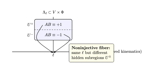
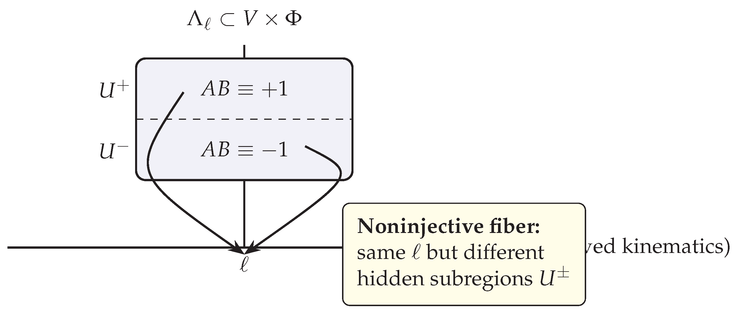
Suppose the hidden state has the form $\Lambda \cong V\times \Phi$ where V is an observed kinematic parameter space and $\Phi$ is an auxiliary PV coordinate. Let $\mathcal{L}:V\times \Phi \to \mathcal{M}$ be an operational kinematic summary (e.g. a Lorentz parameter) that is noninjective on fibers: distinct $(v,\varphi )$ share the same observed $\ell =\mathcal{L}(v,\varphi )$. Then inside a fixed observed cell ℓ, the auxiliary $\varphi$ can carry different sign structure for $A(a,\lambda )B(b,\lambda )$, enabling reweighting without changing the coarse observed kinematics.

Figure 1. PV-style motivation: noninjective hidden fibers allow internal sign structure inside a fixed observed kinematic cell.

Figure 1. PV-style motivation: noninjective hidden fibers allow internal sign structure inside a fixed observed kinematic cell.

7. Experimental Audit Protocol: Estimating Resolved Noncentrality and What it Can Certify

The bound $S_{\mathrm{obs}}\le 2+4\delta$ makes $\delta$ operationally meaningful if one has an independent upper bound on $\delta$ for the actual selection rule.

However, without event-ready trials and/or additional assumptions, $\delta$ is not identifiable from accepted data alone. What can be estimated robustly from auxiliary tags is a resolved noncentrality ${\delta }_X$ that lower-bounds$\delta$.

7.1. Resolved Noncentrality from an Auxiliary Tag

Let $X:\Lambda \to \{1,\dots ,K\}$ be a measurable tag (arrival-time residual bin, spectral bin, pulse-energy bin, etc.). Define the pushforward measures ${\rho }^X$ and ${\nu }_{a,b}^X$ on $\{1,\dots ,K\}$ by

$${\rho }^X\left(i\right)=\rho (X=i),{\nu }_{a,b}^X\left(i\right)={\nu }_{a,b}(X=i).$$

Define the coarse-grained RN derivative on bins

$$w^X(a,b;i):={\displaystyle \frac{{\nu }_{a,b}^X\left(i\right)}{{\rho }^X\left(i\right)}}={\mathbb{E}}_{\rho }[w(a,b,\lambda )\mid X=i]={\displaystyle \frac{Pr(\mathrm{accept}\mid a,b,X=i)}{Pr(\mathrm{accept}\mid a,b)}},$$

(where ${\rho }^X\left(i\right)>0$; ignore empty bins).

Definition 3 

(Resolved noncentrality). Define

$${\delta }_X(a,b):=\sum _{i=1}^K|w^X(a,b;i)-1|{\rho }^X\left(i\right)=2\mathrm{TV}({\nu }_{a,b}^X,{\rho }^X),{\delta }_X:=\underset{a,b}{sup}{\delta }_X(a,b).$$

Theorem 7 (Data-processing inequality: binning can onlydecrease$\delta$)For every tag X and every $(a,b)$,

$${\delta }_X(a,b)\le \delta (a,b),\mathrm{hence}{\delta }_X\le \delta .$$

Moreover, if $X^{\prime }$ refines X (i.e. X is a function of $X^{\prime }$), then ${\delta }_X\le {\delta }_{X^{\prime }}$.

Proof. 

Using Jensen’s inequality and conditional expectation,

$${\delta }_X(a,b)={\mathbb{E}}_{\rho }\left(\left|{\mathbb{E}}_{\rho }[w(a,b,\lambda )-1\mid X]\right|\right)\le {\mathbb{E}}_{\rho }\left({\mathbb{E}}_{\rho }\left[\right|w(a,b,\lambda )-1|\mid X]\right)=\delta (a,b).$$

The refinement monotonicity is the same statement applied to the “forgetful” map from $X^{\prime }$ to X. □

Remark 7 

(Interpretation). Auxiliary-tag binning gives an empirical handle onhow noncentral selection already is at the resolution X, but it doesnotupper-bound the true hidden δ without an additional assumption such as “selection depends on λ only through X” (i.e. w is X-measurable).

7.2. Protocol Overview (Event-Ready Recommended)

P1.

Event-ready trials (if possible). Use heralding to define trials independent of outcomes; otherwise use fixed clock bins and include explicit assumptions about which trials “exist”.

P2.

Record rich auxiliary tags X foralltrials. Examples: local arrival times relative to a trial clock, pulse energy monitor, spectral bin, etc. The goal is to enlarge the observed sigma-algebra so that selection becomes more nearly X-measurable.

P3.

Estimate acceptance rates. For each $(a,b)$ and bin i, estimate $\widehat{Pr}(\mathrm{accept}\mid a,b,X=i)$ and $\widehat{Pr}(\mathrm{accept}\mid a,b)$.

P4.

Compute ${\widehat{\delta }}_X$ with uncertainty. Compute $\widehat{w^X}(a,b;i)$ and then ${\widehat{\delta }}_X(a,b)$ and ${\widehat{\delta }}_X={sup}_{a,b}{\widehat{\delta }}_X(a,b)$. Bootstrap over trials to produce a lower CI ${\widehat{\delta }}_X^{(-)}$ (because it is a lower-bound quantity).

P5.

Report aresolution curve. Repeat with progressively refined tags (larger K / more coordinates) to observe whether ${\delta }_X$ stabilizes or grows.

7.3. Estimators

Let ${\widehat{p}}_i=\widehat{Pr}(X=i)$ estimated from all trials (accepted or not). For each $(a,b)$, estimate

$$\widehat{w^X}(a,b;i):={\displaystyle \frac{\widehat{Pr}(\mathrm{accept}\mid a,b,X=i)}{{\sum }_{j=1}^K\widehat{Pr}(\mathrm{accept}\mid a,b,X=j){\widehat{p}}_j}}={\displaystyle \frac{\widehat{Pr}(\mathrm{accept}\mid a,b,X=i)}{\widehat{Pr}(\mathrm{accept}\mid a,b)}}.$$

Then

$${\widehat{\delta }}_X(a,b):=\sum _{i=1}^K|\widehat{w^X}(a,b;i)-1|{\widehat{p}}_i,{\widehat{\delta }}_X:=\underset{a,b}{sup}{\widehat{\delta }}_X(a,b).$$

7.4. What Can Be Concluded (And What Cannot)

What ${\delta }_X$ can certify.

If ${\widehat{\delta }}_X$ is already large (e.g. exceeds the Tsirelson threshold $0.2071$), then the experiment demonstrably contains strong setting-dependent selection structure at the measured resolution X—strong enough, in principle, to inflate CHSH to quantum-like values.

What is needed to exclude selection-based local explanations.

To exclude strictly local MI models of the “selection inflation” type using the bound $S_{\mathrm{obs}}\le 2+4\delta$, one needs an upper bound ${\delta }^{(+)}$ on the true $\delta$. This requires either:

(i)

a justified sufficiency assumption (e.g. w is X-measurable up to negligible error), so that $\delta \approx {\delta }_X$; or

(ii)

an independent physical/model-based constraint on how $\gamma (a,b,\lambda )$ can vary with unmeasured degrees of freedom.

Decision rule (when an upper bound is available).

If an experiment provides an upper confidence bound ${\widehat{\delta }}^{(+)}$ on $\delta$ (by one of the routes above), and an estimate ${\widehat{S}}_{\mathrm{obs}}$ with standard error ${\sigma }_S$, then a one-sided exclusion test is

$${\widehat{S}}_{\mathrm{obs}}>2+4{\widehat{\delta }}^{(+)}+z_{1-\alpha }{\sigma }_S⟹\mathrm{exclude}\mathrm{local}\mathrm{MI}\mathrm{selection}\mathrm{models}\mathrm{with}\delta \le {\widehat{\delta }}^{(+)}\mathrm{at}\mathrm{confidence}1-\alpha .$$

Window dithering / threshold sweeps (robustness diagnostics).

Repeating the analysis while varying coincidence windows, thresholds, filters, and binning rules is still valuable as a robustness diagnostic: large swings in $\widehat{E}(a,b)$ or $\widehat{S}$ under small analysis perturbations are direct evidence that selection rules matter. But such sweeps do not, by themselves, furnish a rigorous upper bound on $\delta$ without explicit modeling assumptions.

8. Conclusions

Bell–CHSH is correct for unconditional correlations (Theorem 1). Whether an observed CHSH violation compels nonlocality depends on the selection semantics: the accepted correlations are expectations under a potentially setting-dependent measure ${\nu }_{a,b}$.

The RN density w and its $L^1$ deviation from centrality $\delta$ provide a clean quantitative parameterization of this gap. The universal inflation bound

$$S_{\mathrm{obs}}\le min\{4,2+4\delta \}$$

turns “fair sampling” from a slogan into a measurable requirement: Tsirelson’s $2\sqrt{2}$ demands $\delta \ge 0.2071$ somewhere if one insists on strict locality and MI with setting-dependent post-selection.

Rather than asserting a blanket “refutation of local realism” from $S_{\mathrm{obs}}>2$ alone, the defensible scientific program is: (i) formalize selection as a measure-theoretic reweighting, (ii) quantify how much noncentrality is needed to mimic a given CHSH violation, and (iii) audit (or explicitly assume) the selection structure in the experimental pipeline.

Appendix B.1. A Shared Logical Pattern: “Cancellation” Hides a Hypothesis

In the PV note, a CAS output such as

$$v=\pm {\displaystyle \frac{\sqrt{c^{2}D}}{\sqrt{D}}}$$

is only meaningful as a generic expression once one has implicitly bracketed away the exceptional locus $D=0$ (i.e. worked in the localization $D\ne 0$). In strict semantics, the original radical equation forces $D=0$ and therefore cannot determine v.

Bell–CHSH has an analogous inferential fault line: the step from accepted (post-selected) correlations to unconditional correlations, and the step from four different accepted ensembles to a single ensemble, are both cancellation moves valid only under explicit selection hypotheses.

Recall

$$E_{\mathrm{obs}}(a,b)=\int A(a,\lambda )B(b,\lambda )w(a,b,\lambda )\rho \left(d\lambda \right),\int w(a,b,\lambda )\rho \left(d\lambda \right)=1,$$

and $E_{\mathrm{full}}(a,b)=\int A(a,\lambda )B(b,\lambda )\rho \left(d\lambda \right)$.

Lemma A1 

(Measure-identification lemma). Fix $(a,b)$. The following are equivalent:

(i)

${\nu }_{a,b}=\rho$ (equivalently $w(a,b,\lambda )=1$ρ-a.e.).

(ii)

For every bounded measurable $f:\Lambda \to \mathbb{R}$,

$$\int f\left(\lambda \right)d{\nu }_{a,b}\left(\lambda \right)=\int f\left(\lambda \right)d\rho \left(\lambda \right).$$

In particular, equality of asinglecorrelation $\int A(a,\lambda )B(b,\lambda )d{\nu }_{a,b}=\int A(a,\lambda )B(b,\lambda )d\rho$ doesnotimply ${\nu }_{a,b}=\rho$.

Proof. (i)⇒(ii) is immediate. For (ii)⇒(i), equality of integrals for all bounded measurable f implies equality of measures, hence $w=1$$\rho$-a.e. by uniqueness of the RN derivative. □

Appendix B.2. Bell States B0/B1/B3/B4 (the PV-Analogue Template)

We now define four Bell-analogue states, deliberately paralleling the PV note.

Definition A1 

(Bell-state semantics). Fix a Bell-test model class with MI and locality. Define:

• B0 (strict observational semantics).The accepted-sample correlations are computed under theactualsetting-dependent measures $d{\nu }_{a,b}=w(a,b,\lambda )d\rho$, with no assumption that w is setting-independent or central.
• B1 (bracketed / CHSH-applicable semantics).One adds an explicit selection hypothesis sufficient to integrate the CHSH pointwise algebra over a single measure—e.g. setting-independent selection (Definition 1), and in the stronger fair-sampling form, centrality ${\nu }_{a,b}=\rho$ (Definition 2).
• B3 (regularized semantics).One does not assert w is setting-independent or central, but bounds its deviation from centrality by δ and uses the universal inflation bound $S_{\mathrm{obs}}\le min\{4,2+4\delta \}$.
• B4 (blow-up / resolution semantics).One enlarges the observable sigma-algebra by introducing auxiliary tags X (time residual, spectral bin, pulse-energy bin, etc.) so that selection dependence becomes partially resolved and one can estimate ${\delta }_X$ (a lower bound on δ).

Appendix B.3. A Compact Comparison Table (PV S0–S4 vs. Bell B0–B4)

State idea	PV radical note	Bell inference analogue
Strict semantics	S0: original radical equation forces $D=0$, v underdetermined	B0: accepted data governed by setting-dependent ${\nu }_{a,b}$; CHSH can inflate up to $2+4\delta$
Bracket / generic	S1: add $D\ne 0$ to divide by $\sqrt{D}$ and get a determinate v branch	B1: add an explicit selection hypothesis (setting-independence; optionally centrality ${\nu }_{a,b}=\rho$) to apply CHSH$\le 2$ to accepted data
Regularize	S3: assign a continuation across $0/0$ (removable singularity convention)	B3: bound $\delta$ and use $S_{\mathrm{obs}}\le min\{4,2+4\delta \}$ as controlled near-central inference
Resolve / blow-up	S4: add a direction coordinate over the base locus to resolve indeterminacy	B4: add auxiliary tags/partitions to resolve and estimate selection structure (${\delta }_X\le \delta$)

Appendix B.4. Diagram: Where the Extra Hypothesis Enters (Modus Ponens Made Explicit)

Remark A1 

(What this does and does not “critique”). The critique is not that Bell’s theorem is incorrect. It is that the common inference

$$``\mathrm{CHSH}\mathrm{violation}’’\Rightarrow ``\mathrm{nonlocality}’’$$

silently inserts a B1-style selection hypothesis. Without that, the logically correct strict statement is B0/B3:

$$S_{\mathrm{obs}}\le min\{4,2+4\delta \},$$

and Tsirelson’s $2\sqrt{2}$ demands $\delta \ge (2\sqrt{2}-2)/4$ somewhere if one insists on strict locality and MI.

References

- Bell, J. S. On the Einstein Podolsky Rosen Paradox. Physics Physique Fizika 1964, 1, 195–200. [Google Scholar] [CrossRef]
- Clauser, J. F.; Horne, M. A.; Shimony, A.; Holt, R. A. Proposed experiment to test local hidden-variable theories. Phys. Rev. Lett. 1969, 23, 880–884. [Google Scholar] [CrossRef]
- Pearle, P. M. Hidden-variable example based upon data rejection. Phys. Rev. D 1970, 2, 1418–1425. [Google Scholar] [CrossRef]
- Garg, A.; Mermin, N. D. Detector inefficiencies in the Einstein-Podolsky-Rosen experiment. Phys. Rev. D 1987, 35, 3831–3835. [Google Scholar] [CrossRef] [PubMed]
- Eberhard, P. H. Background level and counter efficiencies required for a loophole-free Einstein-Podolsky-Rosen experiment. Phys. Rev. A 1993, 47, R747–R750. [Google Scholar] [CrossRef] [PubMed]
- Hensen, B.; et al. Loophole-free Bell inequality violation using electron spins separated by 1.3 kilometres. Nature 2015, 526, 682–686. [Google Scholar] [CrossRef] [PubMed]
- Giustina, M.; et al. Significant-Loophole-Free Test of Bell’s Theorem with Entangled Photons. Phys. Rev. Lett. 2015, 115, 250401. [Google Scholar] [CrossRef] [PubMed]
- Shalm, L. K.; et al. Strong Loophole-Free Test of Local Realism. Phys. Rev. Lett. 2015, 115, 250402. [Google Scholar] [CrossRef] [PubMed]
Disclaimer/Publisher’s Note: The statements, opinions and data contained in all publications are solely those of the individual author(s) and contributor(s) and not of MDPI and/or the editor(s). MDPI and/or the editor(s) disclaim responsibility for any injury to people or property resulting from any ideas, methods, instructions or products referred to in the content. |
© 2025 by the authors. Licensee MDPI, Basel, Switzerland. This article is an open access article distributed under the terms and conditions of the Creative Commons Attribution (CC BY) license (http://creativecommons.org/licenses/by/4.0/).
Copyright: This open access article is published under a Creative Commons CC BY 4.0 license, which permit the free download, distribution, and reuse, provided that the author and preprint are cited in any reuse.