Submitted:
10 December 2025
Posted:
18 December 2025
You are already at the latest version
Abstract
Fourier Decomposition (FD) and Koopman Mode Decomposition (KMD) are important tools for time series data analysis, applied across a broad spectrum of applications. Both aim to decompose time series functions into superpositions of countably many wave functions, with strikingly similar mathematical foundations. These methodologies derive from the linear decomposition of functions within specific function spaces: FD uses a fixed basis of sine and cosine functions, while KMD employs eigenfunctions of the Koopman linear operator. A notable distinction lies in their scope: FD is confined to periodic functions, while KMD can decompose functions into exponentially amplifying or damping waveforms, making it potentially better suited for describing phenomena beyond FD’s capabilities. However, practical applications of KMD often show that despite accurate approximation of training data, its prediction accuracy is limited. This paper clarifies that this issue is closely related to the number of wave components used in decomposition, referred to as the degree of a KMD. Existing methods use predetermined, arbitrary, or ad hoc values for this degree. We demonstrate that using a degree different from a uniquely determined value for the data allows infinite KMDs to accurately approximate training data, explaining why current methods, which select a single KMD from these candidates, struggle with prediction accuracy. Furthermore, we introduce mathematically supported algorithms to determine the correct degree. Simulations verify that our algorithms can identify the right degrees and generate KMDs that can make accurate predictions, even with noisy data.
Keywords:
Koopman mode decomposition
; uniquely feasible degree
; Hankel matrix
; spectral decomposition
; model selection
; dynamical systems
; time series analysis
1. Introduction
A wide range of natural and social phenomena are observed as superpositions of multiple nonlinear elemental processes. For example, recorded audio signals typically include not only the target speech—for instance, a conversation between individuals—but also various environmental noise components. Similarly, variations in the geomagnetic field arise from both internal processes, such as temporal fluctuations in the Earth’s main magnetic field, and external perturbations, such as solar flares and solar wind. Decomposing such observations into constituent processes and extracting only the components relevant to the study is a fundamental procedure in scientific research. Among such methods, frequency analysis—where time-series data are decomposed into countably (often finitely) many frequency components—plays a central role in data science.
A foundational principle across the natural sciences involves reducing nonlinear phenomena to linear problems, enabling analysis via linear algebra. For instance, kernel methods in machine learning embed data into high-dimensional (often infinite-dimensional Hilbert) spaces to facilitate linear solutions. Likewise, neural networks—which approximate arbitrary continuous (and thus potentially nonlinear) functions via linear combinations followed by nonlinear activations—rely on efficient linear transformations during training. The backpropagation algorithm, essential for learning from large-scale data, exemplifies this reliance.
A well-established and widely applied technique based on this principle is Fourier decomposition, which forms the foundation of frequency analysis across a wide range of fields. Grounded in functional analysis, it represents a function as a linear combination of frequency components, typically expressed in terms of an orthonormal basis of trigonometric functions. This decomposition facilitates tasks such as signal characterization and noise reduction and has found broad applications in speech recognition and compression, image processing, radar and sonar analysis, time-series forecasting, and medical imaging.
Koopman Mode Decomposition (KMD) has recently attracted considerable theoretical attention as a powerful extension of Fourier decomposition. Its origin traces back to the 1931 work of B.O. Koopman, who formulated a representation of nonlinear dynamical systems through linear operators acting on function spaces—now referred to as Koopman operators. The theoretical foundation of this framework was subsequently formalized, and beginning in the 1990s, research by I. Mezić and collaborators renewed interest in its potential to reveal latent dynamics in nonlinear systems. The development of Dynamic Mode Decomposition (DMD) by P.J. Schmid ignited a new wave of research and led to advanced extensions such as Extended DMD (EDMD), which enable practical estimation of Koopman spectral components from data beyond the original limitations of DMD. Although KMD often provides accurate representations of observed data, it has been noted that its predictive accuracy may deteriorate under certain conditions.
The present study aims to address this limitation by identifying the sources of prediction error in KMD and proposing efficient algorithms to extract those Koopman modes that, if present, are the only viable candidates for accurate forecasting.
To illustrate Koopman Mode Decomposition and our contributions, we begin by recalling the concept of Fourier Decomposition (FD). Let be a -periodic, complex-valued function in . That is, for all t, and
The space of such functions forms a Hilbert space, where the inner product between and is defined by
with denoting the complex conjugate of x. Then, admits the decomposition:
This decomposition is justified by the fact that the family
forms a countable orthonormal basis for the Hilbert space of -periodic functions in . The convergence in Equation (1) is understood in the -norm. Although such convergence does not imply pointwise convergence, Riesz’s theorem [1] [Theorem 3.12] guarantees that a subsequence of the partial sums converges pointwise almost everywhere.
Koopman Mode Decomposition (KMD) [2] is similar to FD in that it expresses a function as a sum of oscillatory components. However, unlike FD, KMD allows for exponentially growing or decaying components. Hence, if a KMD of exists, it takes the form:
where . Thus, unless , each term represents an exponentially growing (if ) or decaying (if ) wave (see Figure 1). The constitute a countable subset of the spectrum of the so-called Koopman operator [2].
KMD is expected to provide a more flexible framework for representing diverse phenomena and has been applied in a wide array of domains, including: fluid dynamics [3,4,5,6], chaotic systems [7], neuroscience [8], plasma physics [9,10,11], sports analytics [12], robotics [13], and video processing [14].
In practical settings, both FD and KMD rely on a finite number of observations. Without restricting the summations in Equation (1) and Equation (2) to finitely many terms, the decomposition becomes ill-posed. We therefore approximate the function by a finite superposition of ℓ oscillatory components, where ℓ is called the degree of the decomposition.
In the case of the Discrete Fourier Transform (DFT), we assume observations at , for . Since whenever , the problem of finding the coefficients reduces to solving the linear system:
This system has a unique solution, as the coefficient matrix is a square Vandermonde matrix over distinct T-th roots of unity.
In general, an matrix
is referred to as a Vandermonde matrix, whose determinant when is given by
The square matrix on the right-hand side of Equation (3) is a Vandermonde matrix, and Equation (3) can be restated as
where is a primitive T-th root of unity.
By the aforementioned invertibility of the Vandermonde matrix generated by distinct points , Equation (3) admits a unique solution:
Here, denotes the conjugate transpose (i.e., Hermitian transpose) of a matrix .
In contrast, the KMD problem can be formulated analogously as:
with the following distinctions:
- Each observable is an m-dimensional vector. We denote the matrix of observations by .
- The eigenvalues and the corresponding modes are unknown and must be determined.
- The choice , which is required for DFT, is entirely unsuitable for KMD: for any distinct set of , there always exists a corresponding set of modes such that Equation (6) holds exactly.
Despite the increased complexity of the KMD problem, several numerical methods exist to solve Equation (6) for a given degree ℓ, including: Dynamic Mode Decomposition (DMD), which is typically applicable when ; the Arnoldi method, applicable when ; and the vector Prony method, which allows arbitrary ℓ. These methods yield approximate solutions minimizing the residual sum of squares (RSS), especially in the presence of observation noise.
However, what remained unresolved was how to determine an optimal degree ℓ. We illustrate its importance through the following example, highlighting the predictive risk of inappropriate choice.
Example 1.
Consider one-dimensional observables given by . It is readily verified that Equation (6) admits no solution if . For , the roots of the following equation
uniquely determine the modes such that Equation (6) is satisfied, thereby yielding a valid KMD for any value of the parameter α. As illustrated in Figure 2, all such KMDs exactly reproduce the observed sequence for , yet their extrapolations for differ significantly.
This example highlights a key issue: even if an algorithm happens to return a single quartic KMD, it is merely one among infinitely many KMDs that fit the observed data. Consequently, the forecast made by such a KMD is almost certainly different from the ground truth, and the chance of accurate prediction is negligibly small.
Thus, for the sake of predictive accuracy, it is crucial to select ℓ such that it is uniquely feasible, defined as follows:
Definition 1.
Given an observable matrix , a degree ℓ is said to befeasibleif there exists at least one solution to Equation (6). Moreover, if this solution is unique, then ℓ is said to beuniquely feasible.
This paper develops a theoretical framework for uniquely feasible degrees and, based on this foundation, proposes efficient and practical algorithms to determine whether a given set of observables admits a uniquely feasible degree—and if so, to identify it. We also demonstrate through simulations that the KMD selected by our algorithms can yield highly accurate predictions.
2. Theoretical Frameworks Underlying Koopman Mode Decomposition
A key significance of Koopman Mode Decomposition (KMD) is its ability to analyze the dynamics of a nonlinear system using only methods from linear algebra. In this section, we provide a brief review of the theoretical framework of KMD, which bridges nonlinear dynamics and linear algebra.
2.1. Temporal Transition of States and Semigroup Property
Let Z denote a (possibly unobservable) state space. Under a deterministic assumption, once a state is observed at some time, the state of the system after an elapsed time is uniquely determined and is denoted by . Accordingly, the temporal evolution of the system is described by the mapping
In the discrete-time setting, is instead defined on , which can be regarded as a special case of the continuous-time formulation.
While the notation emphasizes the bivariate nature of the mapping, the map is essentially regarded as a univariate function of t, with the initial state fixed. The deterministic assumption also requires the identity , which is equivalently expressed as
for all . This implies that if we define for , then the family
forms a one-parameter semigroup under composition, that is,
holds for all .
2.2. Koopman Operator
We denote the space of -valued functions defined over Z by . The function space forms a -algebra, equipped with addition, multiplication, and scalar multiplication, defined as follows for and :
In particular, is a vector space over .
The Koopman operator parameterized by time t is defined as
It is straightforward to verify that the Koopman operator is a -algebra homomorphism and, in particular, a linear operator. Furthermore, we have:
Proposition 1.
The collection of Koopman operators forms a one-parameter semigroup. That is, holds for any .
2.3. Koopman Generator
In general, when a one-parameter semigroup is defined on a Banach space , it is said to be strongly continuous if, for every , the following norm convergence holds:
A strongly continuous one-parameter semigroup has several important properties [15] [Chapter 13]:
- Each is bounded; that is, the operator norm is well-defined. More precisely, there exist constants and such that for all .
- The set of all for whichexists is a dense linear subspace of , and A is a closed linear operator with domain . This operator A is called the infinitesimal generator of .
- If is bounded, i.e., , then .
- For every , the derivativeexists, and we havefor all and .
- If for some and (that is, is an eigenvalue of A), then
When we say that the Koopman operator semigroup is strongly continuous, we assume that it acts on a Banach space whose elements can be regarded as functions in in some way (e.g., ), and that for each the limit
holds in the norm of . Pointwise convergence of functions is a more primitive notion, and although these two modes of convergence are generally independent, they are closely related in certain settings.
-
Let X be a compact topological space and let denote the space of continuous functions on X. Since every continuous function on a compact space is bounded, we may equip with the supremum norm:With this norm, is a Banach space. In this setting, convergence in norm is equivalent to uniform convergence, and in particular, uniform convergence implies pointwise convergence.
- Let be a measure space, and let for . Elements of are equivalence classes of measurable functions that are equal almost everywhere. Thus, any statement about pointwise convergence should be interpreted in terms of representatives of these equivalence classes, that is, convergence almost everywhere. If a sequence satisfiesthen there exists a subsequence that converges to f pointwise almost everywhere. This follows from the completeness of spaces and is sometimes referred to as a version of the Riesz convergence theorem (see [1] [Theorem 3.12]).
If the Koopman operator semigroup is bounded, then its infinitesimal generator, referred to as the Koopman generator, and defined by
is defined on the entire Banach space.
We next consider the case in which the Koopman operators are bounded. Let be a measure space, and suppose that for each the map is measurable. We examine the boundedness of the associated Koopman operator acting on .
A sufficient condition for to be bounded on is that is non-expansive with respect to , meaning that
In this case, for any ,
where denotes the pushforward of by . If is non-expansive, then (as measures), and hence
so in particular
(For , the same argument shows .)
Conversely, if is expansive, i.e., there exists such that
then the family may fail to be uniformly bounded in t (even though each fixed can still be bounded).
In many applications, especially in ergodic theory and dynamical systems, is assumed to be measure-preserving, that is,
This implies , and hence acts as an isometry on for every . On , the Koopman operators are therefore unitary. If, in addition, forms a measure-preserving flow (so that is a strongly continuous unitary group), then by Stone’s theorem [1] [Theorem 13.40] the Koopman generator is skew-adjoint, i.e., . Since unitary and skew-adjoint operators are normal, the spectral theorem applies and provides the functional-analytic foundation for the Koopman Mode Decomposition.
2.4. Koopman Mode Decomposition and Spectral Theorem
To introduce the Koopman mode decomposition, we assume that the Koopman operator semigroup defined on a Banach space is strongly continuous in the norm of and induces a Koopman generator defined on the entire . For example, this holds when the semigroup is bounded.
Let denote the point spectrum of , and let be the eigenspace corresponding to . When f belongs to the completion in of the linear span of , that is, when
holds in the norm of , only countably many are nonzero. We denote the corresponding eigenvalues by . Then the Koopman mode decomposition of f is expressed as
and the following relations hold:
If, in addition, every element of the one-parameter semigroup is measure-preserving on a measure space , then the Koopman operators and the Koopman generator defined on are unitary and skew-adjoint, respectively; that is, they are normal linear operators defined on the entire . Hence, the Koopman mode decomposition can be understood in the context of the spectral theorem.
The spectral theorem asserts that a normal operator T defined on a Hilbert space can be represented as
where E is a projection-valued measure, which plays the role of a Borel measure defined on the Borel -algebra of . For each , the value is an orthogonal projection operator on rather than a real number, and the measure E satisfies the following properties:
- Orthogonality: .
- Countable additivity: For any countable mutually disjoint family ,where the convergence is in the strong operator topology.
Based on the projection-valued measure E, the integral of a measurable function F over is defined as
in complete analogy with the Lebesgue integral.
This integral representation is essential, because the spectrum may be distributed continuously in . Furthermore, letting denote the set of all isolated eigenvalues of T, we can express the decomposition as
where each for coincides with the orthogonal projection onto the eigenspace of .
For —an equivalence class of functions equal almost everywhere— the Koopman mode decomposition of f and the actions of the Koopman generator and the Koopman operators are obtained by setting and assuming that the integral part of Equation (9) vanishes (or is negligible). Since is nonzero only for a countable subset of , we label the corresponding eigenvalues as for , and write .
- For , we obtain the Koopman mode decomposition of f:
- For , we obtain the action of :
- For , we obtain the action of :
3. Discrete Koopman Mode Decomposition
The objective of Discrete Koopman Mode Decomposition (DKMD) is analogous to that of the Discrete Fourier Transform (DFT): to obtain a decomposition that fits a given finite sequence of samples of an unknown function. We begin by recalling the formulation of the DFT.
3.1. DFT and Vandelmonde Matrix
Let denote the values of an unknown function observed at times . The DFT seeks coefficients such that
Since this is an underdetermined system with infinitely many unknowns, we restrict to a finite sum. Moreover, since implies , we may assume . Let . Then
In matrix form, we can write
The coefficient matrix above is an instance of the Vandermonde matrix.
Definition 2.
Let and . The associatedVandermonde matrixis defined as
Basic properties. For pairwise distinct nodes , the Vandermonde matrix satisfies:
- .
- .
- Viewing as a linear map , F is injective if and only if , surjective if and only if , and bijective if and only if .
In particular,
so Equation (10) has a unique solution for .
3.2. Formulation of DKMD
Assume that the Koopman mode decomposition of a function f is expressed as a countably infinite sum of eigenfunctions of the Koopman generator . For example, assume that the spectrum of consists only of a countably infinite set of isolated eigenvalues :
Then, without loss of generality, we may assume that the values are pairwise distinct.
Given finitely many samples for , DKMD seeks to satisfy
In the same way as in the DFT case, since the infinitely many unknowns and make the system indefinite, we restrict their number to a finite . Then the system can be written compactly as
If are pairwise distinct and , the Vandermonde matrix represents a surjective linear mapping from onto . Then we have the following:
Proposition 2.
For any , pairwise distinct , and , there exists satisfying Equation (13).
Thus, in contrast to the DFT case, where the given values are decomposed into exactly T Fourier components, performing DKMD requires determining the number ℓ of Koopman modes within the range . Specifically, in the nonlinear system (13), the Koopman degree ℓ itself appears as an additional unknown, alongside and .
In this regard, the primary contribution of this paper is to establish criteria for determining ℓ, and to present computationally efficient methods for estimating it both exactly and approximately, particularly when the given observations are contaminated by noise.
In Section 5, we review an existing method from the literature for solving the equation in the special case where ℓ is known.
4. Definitions and Notations
The following definitions and descriptions are essential for the subsequent sections.
We extend the aforementioned formalization of DKMD from the decomposition of -valued functions to that of -valued functions for a dimension . This modification does not alter the fundamental nature of the problem but better aligns with real-world applications of DKMD, such as fluid dynamics.
Definition 3
(DKMD). Let be a matrix of observables at times , where each is an m-dimensional column vector. The discrete Koopman mode decomposition (DKMD) of this observable matrix is a matrix factorization given by
where are pairwise distinct.
Definition 4
(Koopman Eigenvalues, Modes, and Degree). Given a DKMD as in Equation (14), we refer to ℓ as theKoopman degree, as theKoopman eigenvalues, and as theKoopman modes.
For convenience, let and denote the observable matrix and the matrix of modes, respectively:
Then the DKMD can be expressed compactly as
Table 1 summarizes the principal notations used throughout this article.
5. Computing DKMD for Known Degrees (Related Work)
In this section, we introduce the vector Prony method [16], which estimates the unknown Koopman eigenvalues and the Koopman mode matrix that satisfy Equation (15), given the observable matrix and the Koopman degree ℓ.
The procedure first computes the Koopman eigenvalues, and subsequently computes the Koopman modes based on the obtained eigenvalues.
5.1. Computing the Koopman Eigenvalues
We first introduce the characteristic polynomial associated with a DKMD, whose roots correspond to the Koopman eigenvalues.
Definition 5
(Characteristic Polynomial). For a DKMD , the polynomial
is called thecharacteristic polynomialof the DKMD.
If the characteristic polynomial of a DKMD is expressed as
then the following recurrence relation holds:
Proposition 3.
For all integers j with ,
Proof.
The statement follows from
□
Using Hankel matrices (Definition 6), the statement of Proposition 3 can be compactly expressed as
Definition 6
(Hankel Matrix). Given a matrix , the kth Hankel matrix of is defined for as
where .
Although that satisfy Equation (16) may not exist, and even if they exist they may not be unique, the following least-squares optimality always holds:
This represents the least-squares solution for the characteristic coefficients when Equation (16) is inconsistent.
5.2. Computing the Koopman Modes
Once the eigenvalues are computed, the linear equation (14) determines . Since
holds, if a solution exists, provides one possible solution, which is not necessarily unique.
Equation (15) can be viewed as a factorization of linear mappings:
The condition for the existence of such an is
Under this condition, the solution is unique if and only if is surjective, which holds if and only if and the nodes are pairwise distinct.
Proposition 4.
For an observable matrix and a Koopman degree ℓ with , a DKMD of with Koopman eigenvalues , if it exists, it is unique.
6. The Contributions of This Article
Given an observable matrix, the vector Prony method introduced in the previous section computes a DKMD for a specified Koopman degree ℓ. However, a DKMD does not always exist for the given degree, and even when it does, it may not be unique.
Definition 7
(Feasible Degree). A Koopman degree ℓ is said to befeasiblefor the observables if a DKMD of degree ℓ exists for the given observable matrix.
Although the Koopman degree ℓ must satisfy (Proposition 2), a DKMD may exist for multiple values of ℓ. Thus, selecting the optimal feasible degree is essential to obtain an optimal DKMD.
For this selection, we consider two independent principles:
- Minimality:
- The optimal degree should be the smallest among all feasible degrees. This principle is analogous to Occam’s razor, favoring the simplest representation that adequately explains the observations.
- Uniqueness:
- The optimal degree should correspond to a unique DKMD. If multiple DKMDs exist for a given ℓ, as described in a later section, the set of such decompositions forms a continuum, where different DKMDs yield distinct eigenvalues and modes. Consequently, any particular DKMD extracted from this continuum— such as one obtained by the vector Prony method— may fail to reproduce the true dynamics precisely.
In this article, we demonstrate that if a degree satisfies the uniqueness criterion, it also satisfies the minimality criterion, but the converse does not necessarily hold. Thus, between these two principles, we adopt the uniqueness criterion as the standard for selecting the optimal Koopman degree.
Definition 8
(Uniquely Feasible Degree). A Koopman degree is said to beuniquely feasibleif a DKMD of that degree exists and is unique for the given observables.
In summary, the objective of this paper is to establish a theoretical framework for uniquely feasible degrees. Specifically, we demonstrate and present the following:
- A uniquely feasible degree for a given observable matrix, if it exists, is the smallest among all feasible degrees.
- Several structural properties of uniquely feasible degrees lead to computationally efficient algorithms for determining them.
- These algorithms are further extended to handle noisy observables via least-squares formulations.
7. Finding Uniquely Feasible Degrees
7.1. Key Indices: Hankel Dimension and Codimension
We first summarize the results of the previous sections in a theorem that provides a necessary and sufficient condition for an observable matrix to admit a DKMD.
For notational convenience, we first introduce the following definition.
Definition 9
(Square-free coefficient vector). A vector is called asquare-free coefficient vectorif the algebraic equation
has no repeated roots.
Theorem 1
(Feasibility condition). Let be an observable matrix and . The following statements are equivalent:
- 1.
- admits a DKMD with Koopman degree ℓ; equivalently, ℓ is feasible for .
- 2.
- There exists a square-free coefficient vector satisfying
Proof.
(1 ⇒ 2) Suppose admits a DKMD with Koopman eigenvalues . The coefficient vector of the characteristic polynomial of this DKMD is square-free by the definition of DKMD (Definition 3), and the assertion of Proposition 3 can be restated as
which further implies Equation (17).
(2 ⇒ 1) Let denote the distinct roots of the square-free polynomial We consider and as representing linear mappings , , and , respectively. Then, the rank-nullity theorem implies
and follows from
for all , which implies the existence of H. □
The square-free coefficient vector in Equation (17) lies in the orthogonal complement , which is the subspace of consisting of all vectors orthogonal to every column of . Theorem 1 thus shows that the existence of a DKMD depends on the structure of and its orthogonal complement. This motivates the following key indices.
Definition 10
(Hankel dimension and codimension). Given an observable matrix , the Hankel dimension and codimension of order k () are defined as
Using these indices, we can restate Theorem 1 as follows:
Corollary 1.
For an observable matrix and a Koopman degree , a necessary condition for the existence of an ℓ-degree DKMD of is
However, the condition is not a sufficient condition due to the following two reasons:
- Even if we can find withit may happen that , meaning that the polynomial corresponding to is of degree lower than ℓ, which cannot induce a DKMD of degree ℓ.
- Even ifthe resulting polynomialmay have repeated roots, rendering it unsuitable as a characteristic polynomial.
Our purpose here is to identify a Koopman degree ℓ that admits a unique DKMD. We can represent the condition for a uniquely feasible degree using the Hankel codimension, assuming that ℓ is feasible, that is, an ℓ-degree DKMD exists.
Corollary 2.
For a feasible degree ℓ of an observable matrix with , the following hold:
- 1.
- The DKMD is unique if and only if .
- 2.
- The set of ℓ-degree DKMDs forms a continuum if and only if .
Proof.
Since ℓ is feasible, is non-empty, and there exists a coefficient vector
which determines the characteristic polynomial of a DKMD of .
If , that is, if , then only can determine a characteristic polynomial, implying that the DKMD is unique by Proposition 4.
On the other hand, if , there exists a coefficient vector
When we define
since is square-free, there exists such that remains square-free for any . In particular, each distinct value of yields a distinct DKMD. □
7.2. The Koopman Dimension and Codimension for
In this section, we investigate the Hankel dimension and codimension in the restricted case where , i.e., when consists of a single row with T components. These results will be extended to the general case in Section 7.4.6.
Lemma 1.
Let be an observable matrix with one row and T columns. Furthermore, suppose that admits a DKMD of the form
such that and each is nonzero. Then, the leftmost block submatrix of has nonzero determinant.
Proof.
The leftmost block submatrix is expressed as:
The determinant of this matrix is nonzero, because are mutually distinct, implying and are nonzero, implying . □
Theorem 2.
Let , , and be as in Lemma 1. Assume further that . Then, the Hankel dimension and codimension are given by:
Proof.
Note that consists of rows and columns.
If , equivalently if and , the leftmost submatrix of coincides with the top submatrix of , implying its rank is by Lemma 1. Thus, all rows of are linearly independent, and follows.
If , equivalently if and , the entire has columns. Its top submatrix coincides with the leftmost submatrix of , implying its rank is by Lemma 1. Thus, all columns of are linearly independent, and follows.
If , equivalently if and , the top-left submatrix of coincides with that of , and hence, Lemma 1 implies that the leftmost ℓ columns of are linearly independent.
On the other hand, we let
denote the characteristic polynomial. Then each eigenvalue satisfies . For the i-th element of with ,
This recurrence relation shows that for any , the element is determined by . Consequently, any column of is a linear combination of the leftmost ℓ columns, which have been proven to be linearly independent. Therefore, .
The claims about the Hankel codimension follow directly from the definition . □
Corollary 3.
If , then is the unique value satisfying .
If , then admits no uniquely feasible degree.
7.3. Examples
In this section, we introduce three examples of an observable matrix , each demonstrating different properties regarding the existence of a uniquely feasible degree:
- No Koopman degree ℓ satisfies , meaning that no uniquely feasible degree exists (Example 2).
- A Koopman degree ℓ with exists, but the corresponding characteristic polynomial is not square-free. As a result, a uniquely feasible degree does not exist (Example 3).
- A uniquely feasible degree exists, ensuring that a DKMD is uniquely determined for the degree (Example 4).
These examples illustrate the conditions under which a DKMD is uniquely determined and the role of Hankel codimension in establishing uniqueness.
Example 2.
Consider the observable matrix
The Hankel matrices for are computed as:
These computations yield:
implying that admits no DKMD for these degrees by Corollary 1.
On the other hand, for , we have
It follows that
implying that DKMDs form a continuum by Corollary 2.
For example, for ,
Thus, the possible candidates for characteristic polynomials take the form:
whose discriminant is computed as:
Since has no repeated roots if and only if , it follows that 4-degree DKMDs form a continuum.
Example 3.
When we let , the Hankel matrices for are computed as:
implying
In fact, we have , and furthermore,
This implies that there exists no DKMD for any of these degrees because:
- 1.
- For , no characteristic polynomial exists.
- 2.
-
For , if a DKMD existed, the corresponding characteristic polynomial would bewhich is not square-free.
- 3.
-
For , if a DKMD existed, the corresponding characteristic polynomial would be of the formwhich is also not square-free.
On the other hand, for , we have and
implying that there exists a DKMD whose characteristic polynomial is
Furthermore, all possible characteristic polynomials of DKMDs for these observables are of the form
Since is square-free for , and since the set of for which is square-free is an open subset of , we conclude that the set of possible four-degree DKMDs for forms a continuum.
Example 4.
We expand of Example 2 by adding one more dimension to the observables. Let the observable matrix be given by
For , the corresponding Hankel matrices are computed as:
implying
On the other hand,
follows from
Therefore, if admits a uniquely feasible degree, it must be four. In fact,
holds, and the corresponding characteristic polynomial is
which is square-free, implying that is uniquely feasible.
7.4. Important Properties of The Hankel Dimension and Codimension
In this subsection, we introduce important properties of the Hankel dimension and Hankel codimension, which play a crucial role in designing algorithms to determine uniquely feasible degrees, including the following. For the convenience of description, we denote the minimum feasible degree as:
Best Possible Upper Bound of a Uniquely Feasible Degree.
Let . If , then . Hence, no uniquely feasible degree can exceed , which is also the sharpest possible upper bound.
Monotonic Increase of the Hankel Codimension.
The Hankel codimension is strictly increasing with respect to ℓ over the interval .
Equivalence Between Unique and Minimal Feasibility.
The monotonicity of the codimension implies that, if ℓ is uniquely feasible, then . In particular, if , no uniquely feasible degree exists.
Saturation of the Hankel Dimension.
If and , then
In particular, holds, which implies L is the only candidate for a uniquely feasible degree.
7.4.1. Invariance under Basis Transformations
For , , and , we assume
Their corresponding Hankel matrices are computed as
where is defined as the matrix given by
This implies, in particular,
Furthermore, if a square-free polynomial is a characteristic polynomial of a DKMD for , it is also a characteristic polynomial of a DKMD for . In fact, we have
Furthermore, if in addition there exists such that then
holds, and the correspondence of characteristic polynomials is bijective.
The condition for is that the row space of is contained in the row space of , and symmetrically, the condition for is that the row space of contains the row space of . Hence, both and hold if and only if the row space of and the row space of are identical. In other words, under the hypothesis , the necessary and sufficient condition for the existence of such that is .
If and hold, the minimum is zero, and hence, holds, implying
Furthermore, this bijective correspondence between characteristic polynomials yields a bijective correspondence between DKMDs. In fact, which is a DKMD of , yields
which is a DKMD of . In reverse, a DKMD of corresponds to a DKMD of
The latter correspondence is the inverse of the former by Proposition 4.
Thus, we have:
Theorem 3.
If holds for , then the following statements hold:
- 1.
- for each .
- 2.
- for each .
- 3.
- The set of characteristic polynomials for is identical with that for .
- 4.
- A DKMD of can be converted to a DKMD of , while a DKMD of can be converted to a DKMD of . These conversions yield a bijective correspondence between the set of DKMDs for and that for .
As an application of Theorem 3, the following two cases are particularly important:
- When is a nonsingular matrix, we have automatically, and thus Theorem 3 provides the invariance of the Hankel dimension, Hankel codimension, characteristic polynomials, and DKMDs under basis transformations in .
- When with is selected to satisfy , the matrix has fewer rows than , and thus requires less computation to obtain DKMDs than .
7.4.2. Invariance under Basis Transformations
For , , and , we assume
Their corresponding Hankel matrices are computed as
where is defined as the matrix given by
This implies, in particular,
Furthermore, if a square-free polynomial is a characteristic polynomial of a DKMD for , it is also a characteristic polynomial of a DKMD for . In fact, we have
Furthermore, if there exists such that
holds, and the correspondence of characteristic polynomials is bijective.
The condition for is that the row space of is contained in the row space of , and symmetrically, the condition for is that the row space of contains the row space of . Hence, both and hold, if and only if the row space of and the row space of are identical. In other words, under the hypothesis , the necessary and sufficient condition for the existence of such that is .
If and hold, the minimum is zero, and hence, holds, implying
Furthermore, the aforementioned bijective correspondence between characteristic polynomials yields a bijective correspondence between DKMDs. In fact, which is a DKMD of , yields
which is a DKMD of In reverse, a DKMD of corresponds to a DKMD of
The latter correspondence is the inverse of the former by Proposition 4.
Thus, we have:
Theorem 4.
If holds for , then the following statements hold:
- 1.
- for each .
- 2.
- for each .
- 3.
- The set of characteristic polynomials for is identical with that for .
- 4.
- A DKMD of can be converted to a DKMD of , while a DKMD of can be converted to a DKMD of . These conversions yields a bijective correspondence between the set of DKMDs for and that for .
As application of Theorem 3, the following two cases are particularly important.
- When is a nonsingular matrix, we have automatically, and thus Theorem 3 provides the invariance of the Hankel dimension, Hankel codimension, characteristic polynomials and DKMDs under basis transformation in .
- If can be selected to satisfy . since has fewer rows than , requires less computation to obtain DKMDs than .
7.4.3. The Best Possible Upper Bound for A Uniquely Feasible Degree
Although we have seen that a uniquely feasible degree is always less than T, we can determine the best possible upper bound. First, we see:
Proposition 5.
For an observable matrix with T columns, we have if admits a uniquely feasible degree.
Proof.
If ℓ is a uniquely feasible degree, Proposition 2 implies . On the other hand, implies . The assertion follows. □
Based on this Proposition, we now establish the best possible upper bound for a Koopman degree that admits a unique DKMD.
Theorem 5.
If , then . Furthermore, is the best possible upper bound for a uniquely feasible degree.
Proof.
When we take with , Theorem 3 implies
equivalently,
Since by hypothesis, , which yields
To show that is the best possible upper bound for a uniquely feasible degree, we construct an observable matrix with and .
First, we determine a sufficiently long series with mutually distinct eigenvalues and nonzero modes :
where is chosen sufficiently large so that we can construct an observable matrix
Without loss of generality, we let and further suppose for .
We now verify that the columns of correspond exactly to the first columns of . The i-th row of contributes consecutive columns to , where the last such column is . On the other hand, the first column contributed by the -th row is . Since implies , we have , which means the columns contributed by the i-th and -th rows are contiguous (or overlapping) in , with no gaps. Consequently, the set of columns of coincides exactly with the first columns of .
Thus, holds if and only if
by Theorem 2. Since satisfies , the condition for such an to exist is that
Since ℓ must be an integer, the largest feasible value is , completing the proof. □
7.4.4. Monotonic increase of the Hankel codimension
In this section, we establish that the Hankel codimension increases strictly monotonically beyond a certain threshold. This property plays a crucial role in identifying uniquely feasible degrees.
Theorem 6.
In the domain , is strictly monotonically increasing.
Proof.
Let . First, for a nonzero vector , define
This is a nonzero vector in , so we have .
Next, let be a basis of , where . By reordering if necessary, we may assume that
holds for all .
We claim that the following vectors are linearly independent:
which all belong to . To prove the claim, let us consider
The vector has the form , so its -th component equals .
First, we prove for by backward induction on s.
For , consider the -th component of the left-hand side. Among all vectors in the sum, only has a nonzero value at this position, namely . The vectors for have the form , and since , we have , which implies that their -th component is zero. Similarly, for , the vector has nonzero components only up to position , so its -th component is also zero. Therefore, , which gives .
For , assuming by the induction hypothesis, we consider the -th component of the left-hand side. By the same argument as above, only has a nonzero value at position , namely . Therefore, , which gives .
This reduces the equation to , which implies for by the linear independence of .
Therefore,
which completes the proof. □
7.4.5. Equivalence Between Unique and Minimal Feasibility
If a uniquely feasible degree exists, it must coincide with the minimum feasible degree L. This conclusion follows directly from Theorem 6 as an immediate corollary.
Corollary 4.
If admits a uniquely feasible degree, it must be L.
Proof.
While Corollary 2 states that a uniquely feasible degree ℓ must satisfy , Theorem 6 ensures that this condition is met only when . □
7.4.6. Saturation of
In this section, we present a theorem that extends Theorem 2. This result plays a crucial role in the development of algorithms for determining uniquely feasible degrees, particularly in the case where for the minimum feasible degree L.
Theorem 7.
If and an L-degree DKMD exists, then:
Proof.
We express the L-degree DKMD given by hypothesis in the form
No column of is a zero vector, since L is the minimum feasible degree. Indeed, if
held for some , then the coefficient vector
of the polynomial
would belong to , contradicting the definition of L.
By Theorem 3, we can transform by multiplying a matrix such that without changing the assertion. In particular, we may assume the following:
- with . To achieve this, take such that the rows are linearly independent. Then, define so that the j-th row of has 1 as the -th component and 0 for the other components.
- The first row of has no zero component: for . Since each column of is nonzero and , we can find a nonsingular matrix such that the first row of has no zero component.
After this transformation, we apply Theorem 2 to the first row of :
and obtain
since the columns of are among those of . For , in particular, the equality holds because by definition.
Leveraging this evaluation of lower bound, the claim for can be proven by induction on ℓ.
For the base case , the definition of L gives , which implies . Combined with shown above, we have .
For the inductive step, assume and , i.e., . By Theorem 6, , which gives
and consequently, . Combined with , we conclude .
Finally, the expressions for follow directly from the definition of the Hankel codimension. □
Although Theorem 7 requires , if (which occurs only when T is odd), then holds, implying that the range in Theorem 7 is empty. In this boundary case, the theorem provides information only for , namely that and in this range.
For , which for integer L is equivalent to , we have:
Corollary 5.
If L is feasible and satisfies , then L is a uniquely feasible degree.
Proof.
Since L is feasible, an L-degree DKMD exists. The condition implies , so Theorem 7 applies and gives . By Corollary 2, this means that L is uniquely feasible. □
8. Algorithms
Leveraging the five properties mentioned in Section 7.4, we develop efficient algorithms to search for a uniquely feasible degree L and to determine an L-degree characteristic polynomial, which provides eigenvalues of a DKMD. Once mutually distinct eigenvalues are obtained, the associated Koopman modes are calculated as described in Section 5.2. Our algorithms are categorized into:
- One that applies to the case where and determines L by ;
- Another that performs a binary search to determine L in the case when .
To introduce the algorithms, we start by addressing a theoretical scenario where the observables exactly consist of a finite number of wave components. In this case, an exact DKMD is obtained. Subsequently, we consider a practical scenario where the observables comprise a finite number of dominant wave components, an infinite number of minor wave components, and noise. Here, our algorithms focus on extracting only the dominant wave components, effectively filtering out the minor components and the noise, resulting in an approximate DKMD.
8.1. A Theoretical Scenario
We first present Algorithm 1, which reduces the dimension of each observable so that decomposing the reduced observable matrix is equivalent to decomposing the original one. This reduction is practically useful for more efficient computation and clearer understanding of the underlying structure. We then present algorithms that decompose an observable matrix for two cases: (Algorithms 2 and 3) and (Algorithm 4).
8.1.1. Dimension Reduction
Although each observable vector, i.e., a column vector of , is of dimension m, the rank r of can be smaller than m. In this case, Algorithm 1 determines a dimensionally reduced observable matrix and a conversion matrix such that and . By Theorem 3, the Hankel dimensions and codimensions, as well as the set of characteristic polynomials, are invariant under this conversion, and DKMDs for and those for are mutually converted by matrix multiplication by and .
Such and can be constructed by selecting r linearly independent rows of and defining so that these rows become the rows of . Since these r rows of are linearly independent and form all the rows of , we have .
| Algorithm 1 Dimension reduction of the observable matrix. |
|
By applying Algorithm 1, we can reduce the problem of decomposing to the problem of decomposing with . This reduction provides benefits in terms of computational efficiency and clearer understanding of the data structure when executing the algorithms presented below. However, these algorithms are formulated in general terms and do not require that such a dimension reduction has been performed.
8.1.2. Case
Algorithm 2 first investigates whether by leveraging the equivalence between and . Indeed, if , then holds by Theorem 6. Conversely, if , then by the definition of L.
If this investigation reveals , the algorithm identifies L as by Theorem 7, and then executes Algorithm 3 to determine whether L is uniquely feasible. If , the algorithm returns the value continue, indicating that Algorithm 4 should be used.
When invoked, Algorithm 3 verifies the following:
- A vector exists in . This can be efficiently verified by performing a QR decomposition of .
- If such a vector exists, verify that the polynomialhas no repeated roots.
If both conditions are satisfied, this confirms that L is feasible, and we can then apply Theorem 7. As a result, we have , meaning that L is uniquely feasible. Thus, the polynomial obtained in the verification is square-free and serves as the characteristic polynomial of the unique L-degree DKMD of . In this case, the algorithm returns the obtained characteristic polynomial. Otherwise, it returns the value no_solution, indicating that no uniquely feasible degree exists.
| Algorithm 2 Search for an L-degree characteristic polynomial when . |
|
| Algorithm 3 Determine the characteristic polynomial. |
|
8.1.3. Case
Algorithm 4 details the procedure for cases when . Note that if L is uniquely feasible, then holds by Theorem 5, and this gives the best possible upper bound.
The algorithm first verifies whether . If this condition does not hold, no uniquely feasible degree exists, and the algorithm returns the signal no_solution.
If , then L lies in the range . The algorithm utilizes a binary search to find L, leveraging the fact that is a strictly increasing function by Theorem 6.
Since the identified L does not necessarily satisfy , the algorithm must verify before executing Algorithm 3 to confirm that L is uniquely.
8.2. A Practical Scenario
In practice, even if the Koopman operator has only discrete eigenvalues, the number of eigenvalues can be infinite, and in addition, observables can contain error signals. In such situations, the purpose of DKMD is to find a finite number of major wave components that most significantly affect the observables. From the viewpoint of executing our algorithms, the presence of minor components and errors makes direct computation of Hankel dimensions via QR decomposition impractical. In fact, may always hold, which makes it impossible to identify the Hankel dimensions. In this section, we present a method to estimate Hankel dimensions for the major components via singular value decomposition (SVD) rather than QR decomposition.
We assume that the observables are represented as
where and represent major and minor wave components, respectively, and is noise. We define:
and our basic assumption is that is a small perturbation. Our aim is to estimate from , taking advantage of the fact that equals the number of positive singular values of .
| Algorithm 4 Search for an L-degree characteristic polynomial when . |
|
We consider with . Let , , and be the singular values of , , and , respectively. Then,
holds for all . This can be proven as follows. By the Courant–Fischer min-max theorem [17], the i-th singular value of satisfies
Since , we have as follows:
By the same reasoning, we also obtain .
Furthermore, if , that is,
then we have
Therefore, if is sufficiently larger than , there exists a large gap between for and for , and hence, we can estimate r from . Thus, if we can assume that the smallest positive singular value of is sufficiently larger than the largest singular value of , we can apply this method to estimate .
8.3. Time Complexities
The computationally intensive operations in these algorithms primarily involve executing QR decomposition (QRD), singular value decomposition (SVD), and solving equations (EqS). Table 2 demonstrates that the algorithms execute these computations only a small number of times, and consequently, prove to be highly efficient.
9. Simulations
Through simulations, we investigate the accuracy of Algorithms 2 to 4 in estimating Koopman eigenvalues and making predictions.
9.1. Synthetic Datasets Used in the Simulations
The synthetic datasets of observables are constructed with and , which makes a matrix, and are randomly generated by performing the following steps:
-
Sample as many distinct Koopman eigenvalues, each classified as either major or minor, as specified in Table 3. Let denote these eigenvalues. For each , its complex conjugate must also be in the set. Furthermore, every conjugate pair is sampled independently as follows:
- is sampled according to a log-normal distribution with parameters and , whose probability density function is . The median, mean, and variance of this distribution are , , and , respectively.
- is sampled uniformly from the interval .
The distribution of is designed to restrict the occurrence of samples too far from 1, because much larger than 1 causes the observables to diverge, while a component with much smaller than 1 decays rapidly. -
Determine the Koopman mode corresponding to with the following constraints:
- and hold whenever ;
- The modes associated with the major eigenvalues must have significant magnitudes, while those associated with the minor eigenvalues must have smaller magnitudes.
To satisfy the second requirement, we use a function defined below, which has sharp peaks only at the sampled major eigenvalues :For each Koopman eigenvalue , the mode is determined by sampling the argument of each component uniformly at random, while setting the magnitude to , i.e., . - Construct as . If the inclusion of noise is required, add to a noise matrix with and , where each is independently sampled from a normal distribution .
In addition, to evaluate the predictive accuracy of our algorithms, we compute observable values for using the Koopman eigenvalues and Koopman modes determined above.
9.2. Simulation Scenarios
We conduct simulations under the following four distinct scenarios:
- Scenarios 1 and 2 investigate the case where an exact DKMD is obtained via QR decomposition (Section 8.1).
- Scenarios 3 and 4 investigate the case where an approximated DKMD is obtained via singular value decomposition (Section 8.2).
- Scenarios 1 and 3 are used to investigate Algorithm 2.
- Scenarios 2 and 4 are used to investigate Algorithm 4.
9.3. Results of the Simulations
We have obtained excellent results in the simulations for all scenarios. In the case of estimating an exact DKMD, the estimated Koopman eigenvalues and the predictions for are identical to the ground truth within numerical precision. In the case of estimating an approximated DKMD, the estimated Koopman eigenvalues and the predictions for show close agreement with the ground truth.
- Scenarios 1 and 2:
- For both scenarios, Algorithms 2 and 4 correctly identify the ground truth uniquely feasible degrees. Furthermore, we observe that the estimated eigenvalues (the upper-right panels of Figure 3(a,b)) and the predictions for (the bottom panels of Figure 3(a,b)) are identical to the ground truth within numerical precision.
- Scenario 3:
- The upper-left panel in Figure 4(a) depicts the logarithm of the singular values of . Evidently, we observe a significant gap between the top ten singular values and those that follow, leading to the conclusion that , indicating that is the uniquely feasible degree. Furthermore, the estimated eigenvalues (the upper-right panel) and the predictions (the bottom panels) show excellent agreement with the ground truth.
- Scenario 4:
- The upper-left panel in Figure 4(b) depicts the result of a singular value decomposition of when the binary search of Algorithm 4 visits . Since the top 30 singular values are significantly greater than those that follow, we can conclude that , meaning that is the uniquely feasible degree. The estimated eigenvalues and the predictions also show excellent agreement with the ground truth.
10. Conclusions
We have developed a theoretical framework to estimate the correct degree (uniquely feasible degree) of Discrete Koopman Mode Decomposition (DKMD) from a given dataset of observables. The degree of DKMD corresponds to the number of Koopman eigenvalues involved. We demonstrate that unless the correct degree is used, infinitely many DKMDs with different Koopman eigenvalues and modes can fit the training data. However, these variations lead to divergent predictions for future time steps, resulting in unreliable forecasts. Furthermore, the theory provides efficient algorithms to identify uniquely feasible degrees.
References
- Rudin, W. Real and Complex Analysis, 3rd ed.; McGraw-Hill: New York, 1987. [Google Scholar]
- Koopman, B.O. Hamiltonian systems and transformation in Hilbert space. Proceedings of the national academy of sciences of the united states of america 1931, 17, 315. [Google Scholar] [CrossRef] [PubMed]
- Schmid, P.J. Dynamic mode decomposition of numerical and experimental data. Journal of fluid mechanics 2010, 656, 5–28. [Google Scholar] [CrossRef]
- Rowley, C.W.; Mezić, I.; Bagheri, S.; Schlatter, P.; Henningson, D.S. Spectral analysis of nonlinear flows. Journal of Fluid Mechanics 2009, 641, 115–127. [Google Scholar] [CrossRef]
- Tu, J.H.; Rowley, C.W.; Luchtenburg, D.M.; Brunton, S.L.; Kutz, J.N. On dynamic mode decomposition: Theory and applications. Journal of Computational Dynamics 2014, 1, 391. [Google Scholar] [CrossRef]
- Taira, K.; Brunton, S.L.; Dawson, S.T.; Rowley, C.W.; Colonius, T.; McKeon, B.J.; Schmidt, O.T.; Gordeyev, S.; Theofilis, V.; Ukeiley, L.S. Modal analysis of fluid flows: An overview. Aiaa Journal 2017, 55, 4013–4041. [Google Scholar] [CrossRef]
- Brunton, S.L.; Brunton, B.W.; Proctor, J.L.; Kaiser, E.; Kutz, J.N. Chaos as an intermittently forced linear system. Nature communications 2017, 8, 1–9. [Google Scholar] [CrossRef] [PubMed]
- Brunton, B.W.; Johnson, L.A.; Ojemann, J.G.; Kutz, J.N. Extracting spatial–temporal coherent patterns in large-scale neural recordings using dynamic mode decomposition. Journal of neuroscience methods 2016, 258, 1–15. [Google Scholar] [CrossRef] [PubMed]
- Taylor, R.; Kutz, J.N.; Morgan, K.; Nelson, B.A. Dynamic mode decomposition for plasma diagnostics and validation. Review of Scientific Instruments 2018, 89, 053501. [Google Scholar] [CrossRef] [PubMed]
- Kaptanoglu, A.A.; Morgan, K.D.; Hansen, C.J.; Brunton, S.L. Characterizing magnetized plasmas with dynamic mode decomposition. Physics of Plasmas 2020, 27, 032108. [Google Scholar] [CrossRef]
- Kusaba, A.; Shin, K.; Shepard, D.; Kuboyama, T. Predictive Nonlinear Modeling by Koopman Mode Decomposition. In Proceedings of the 2020 International Conference on Data Mining Workshops (ICDMW), 2020; IEEE; pp. 811–819. [Google Scholar]
- Fujii, K.; Takeishi, N.; Kibushi, B.; Kouzaki, M.; Kawahara, Y. Data-driven spectral analysis for coordinative structures in periodic human locomotion. Scientific reports 2019, 9, 1–14. [Google Scholar] [CrossRef] [PubMed]
- Berger, E.; Sastuba, M.; Vogt, D.; Jung, B.; Ben Amor, H. Estimation of perturbations in robotic behavior using dynamic mode decomposition. Advanced Robotics 2015, 29, 331–343. [Google Scholar] [CrossRef]
- Takeishi, N.; Kawahara, Y.; Yairi, T. Sparse nonnegative dynamic mode decomposition. In Proceedings of the 2017 IEEE International Conference on Image Processing (ICIP), 2017; IEEE; pp. 2682–2686. [Google Scholar]
- Rudin, W. Functional Analysis. In McGraw-Hill Series in Higher Mathematics, second ed. Second edition; McGraw-Hill, Inc.: New York, St. Louis, San Francisco, 1991; p. xvi + 424. [Google Scholar]
- Susuki, Y.; Mezic, I. A Prony approximation of Koopman mode decomposition. In Proceedings of the 2015 54th IEEE Conference on Decision and Control (CDC), 2015; IEEE; pp. 7022–7027. [Google Scholar] [CrossRef]
- Horn, R.A.; Johnson, C.R. Matrix Analysis, 2nd ed.; Cambridge University Press, 2012. [Google Scholar]
Figure 1.
Comparison between FD and KMD.
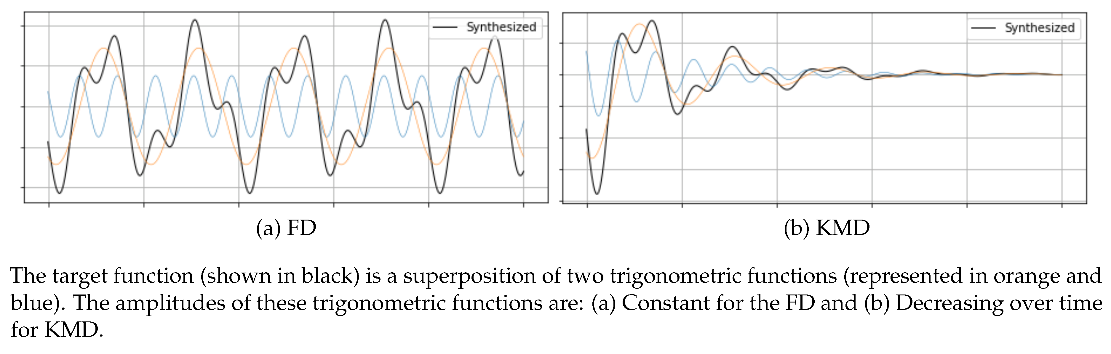
Figure 2.
Illustration of multiple valid KMDs with divergent predictions.
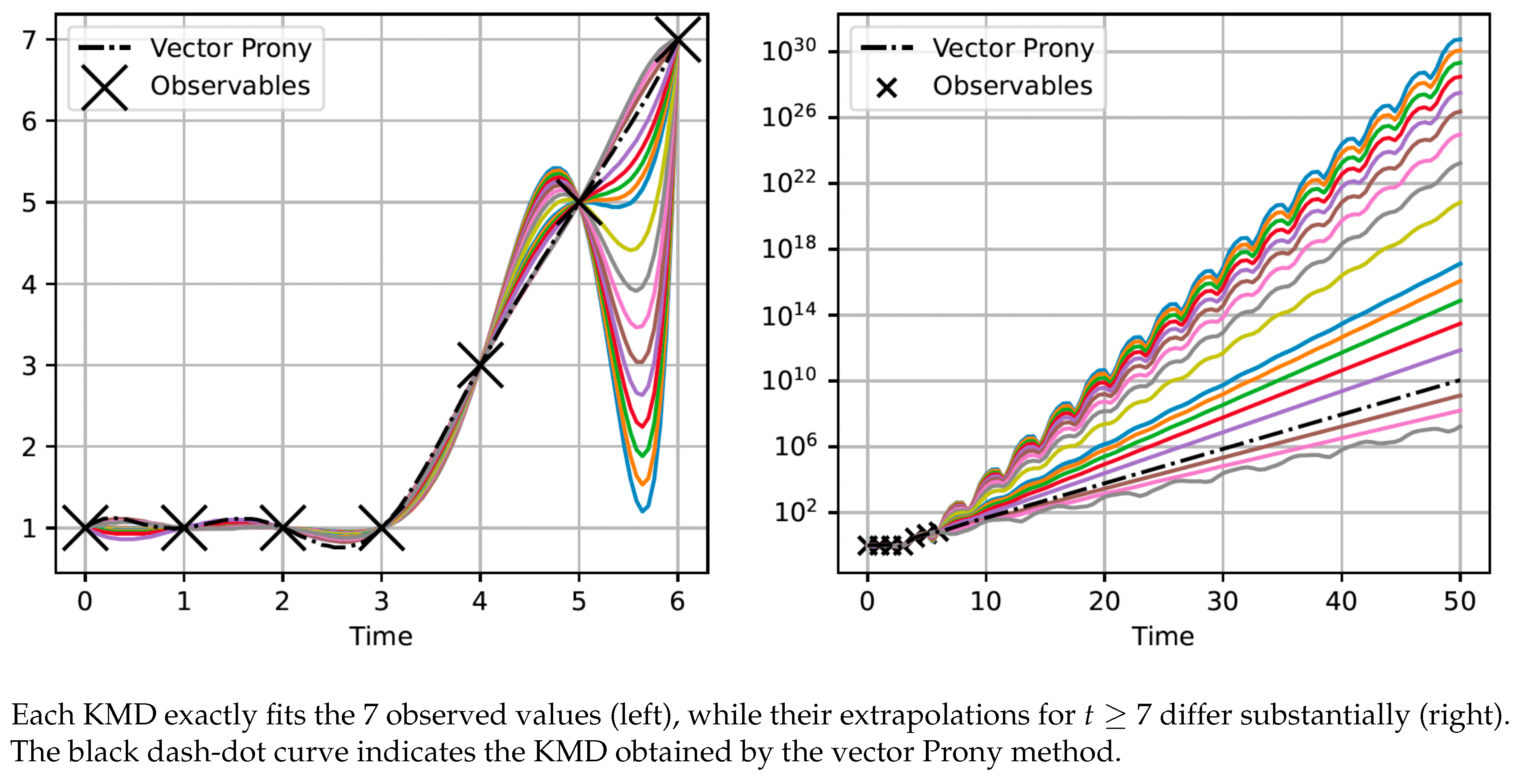
Figure 3.
Results of simulations for Scenarios 1 and 2.
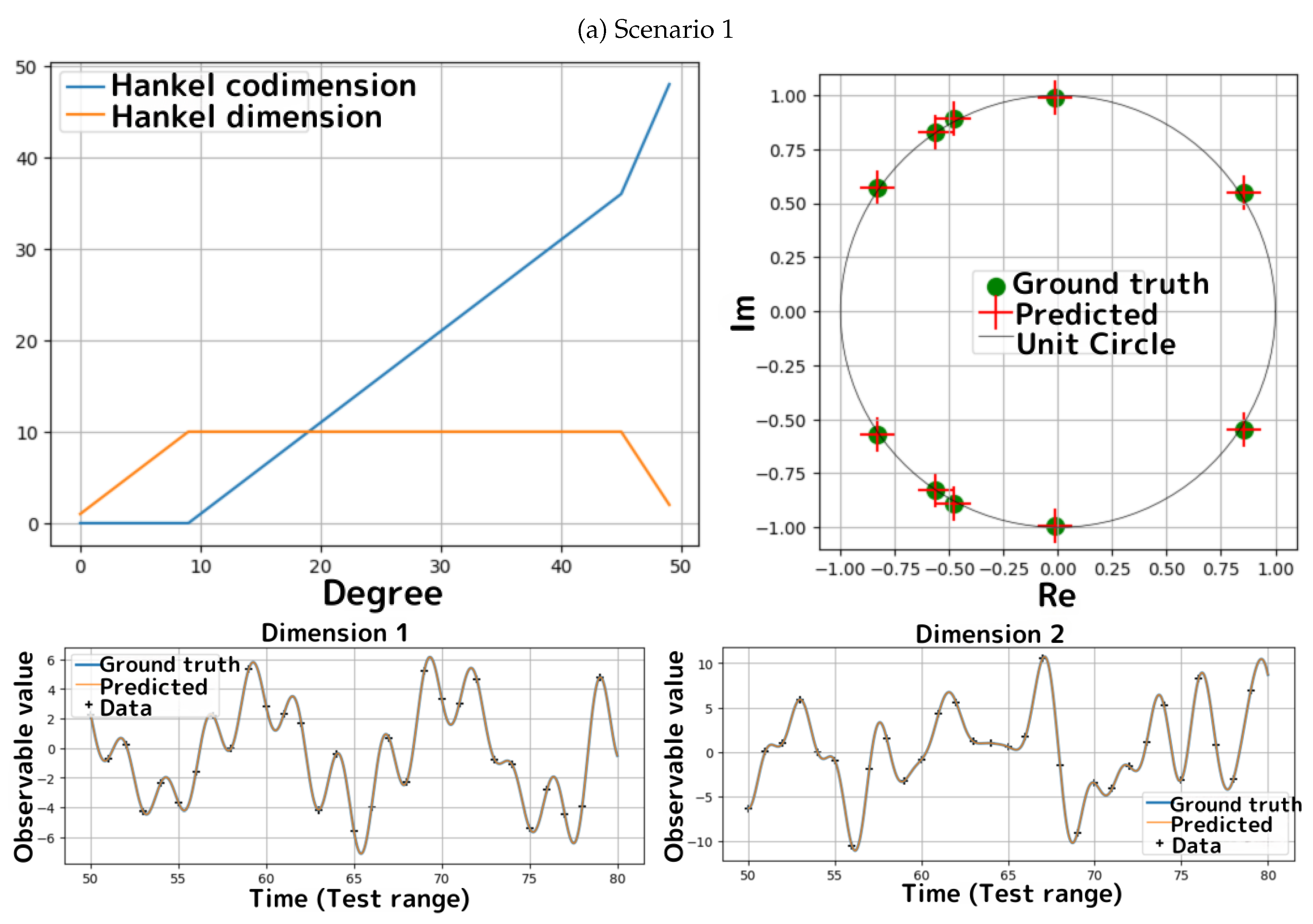
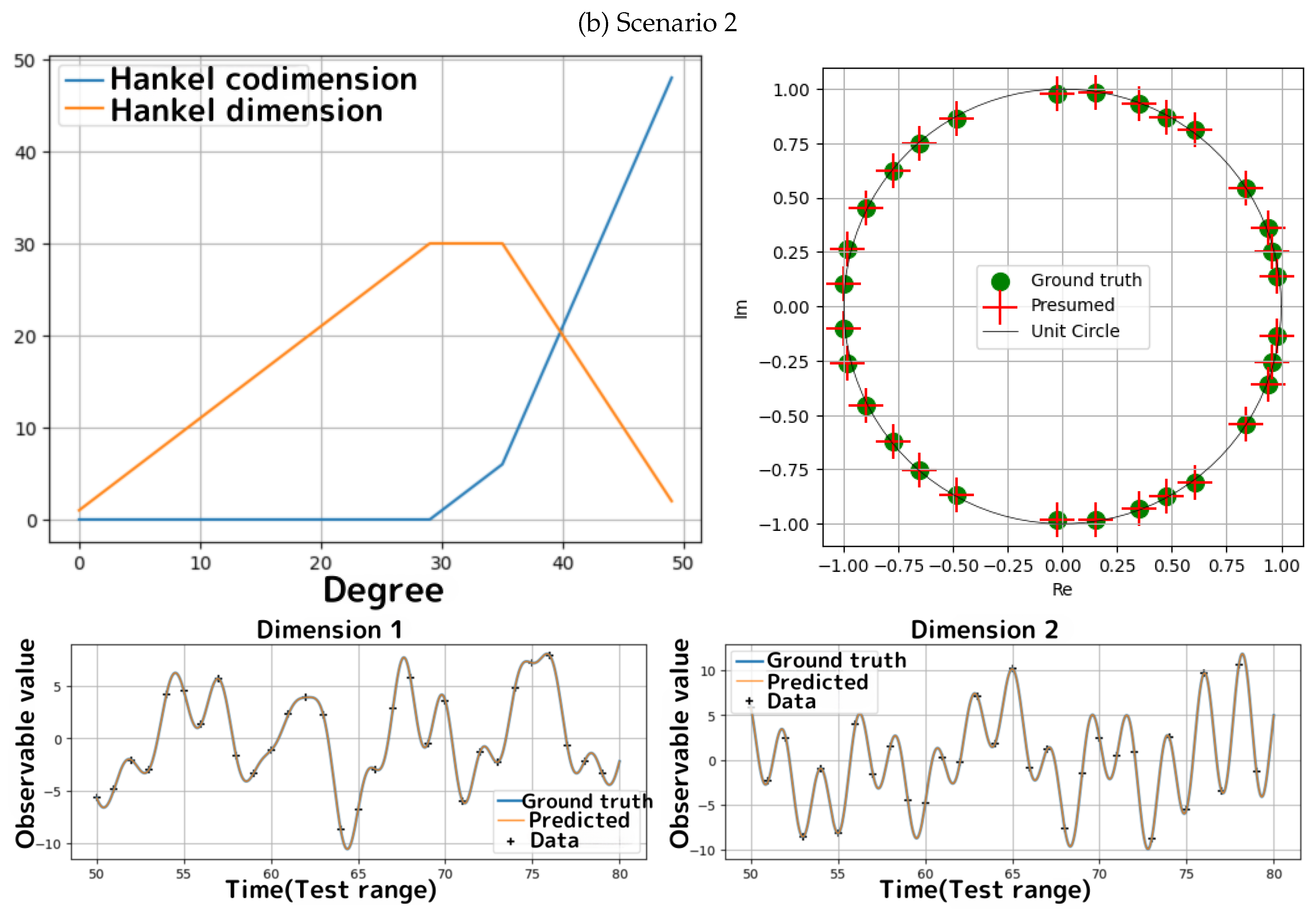
Figure 4.
Results of simulations for Scenarios 3 and 4.
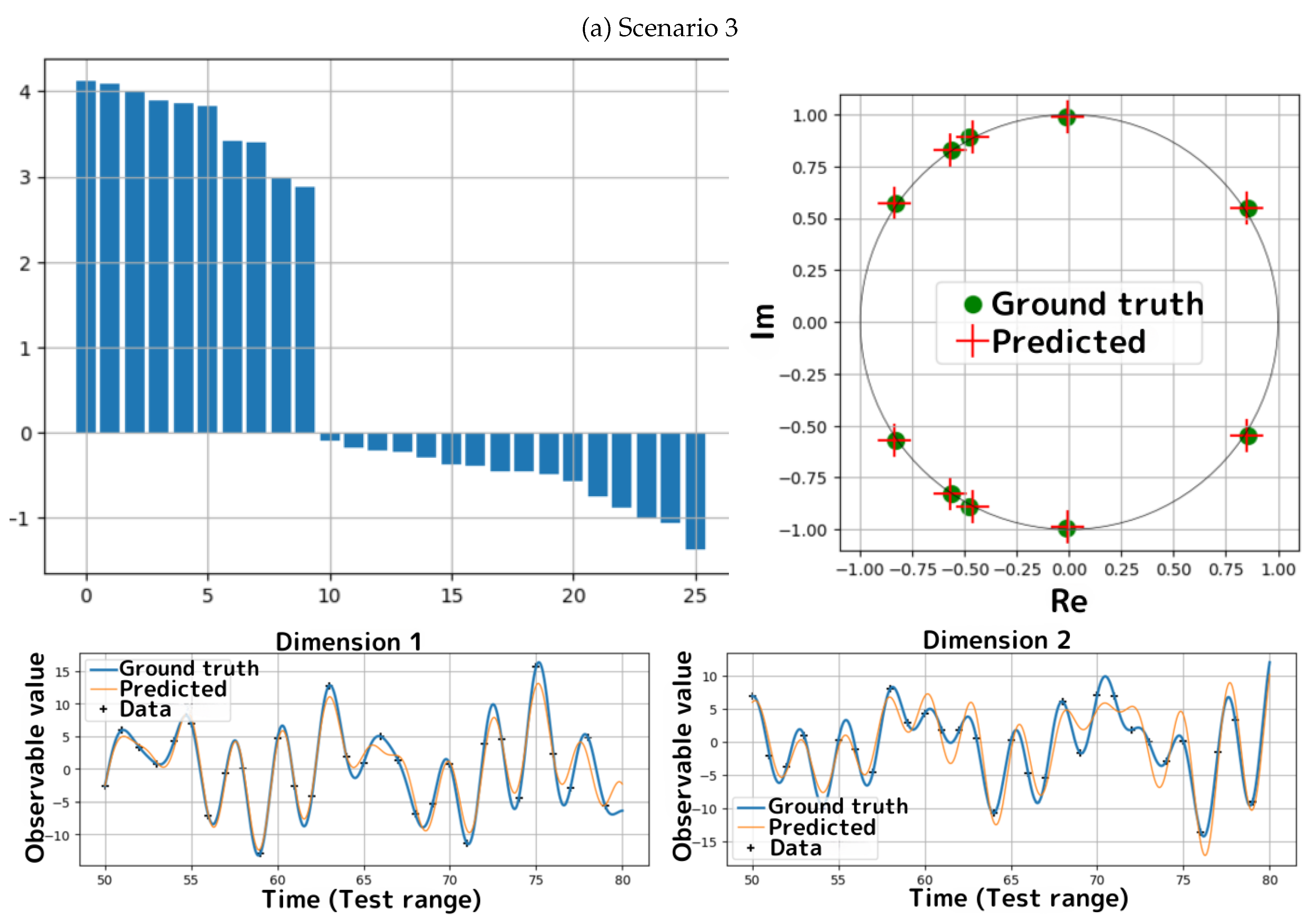
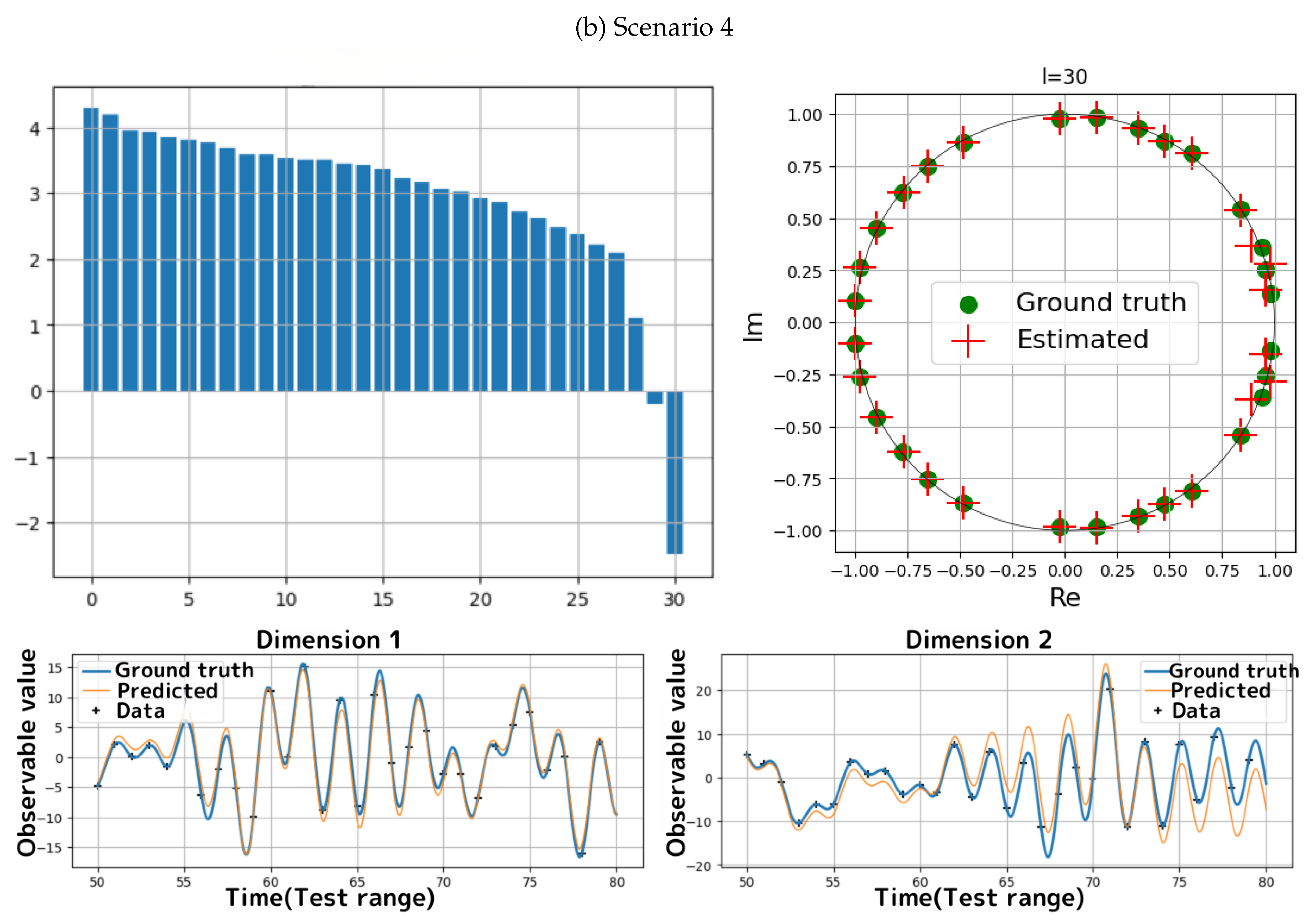

Table 1.
Notation summary.
| Notation | Description |
|---|---|
| ℓ | Koopman degree. |
| Column vectors of observables. | |
| Koopman eigenvalues of an ℓ-degree DKMD. | |
| Koopman modes of an ℓ-degree DKMD. | |
| Observable matrix . | |
| Mode matrix . | |
| Submatrix for . | |
| The ith row vector of . | |
| Vandermonde matrix (Definition 2). | |
| Hankel matrix (Definition 6). | |
| kth Hankel dimension of , defined as (Definition 10). | |
| kth Hankel codimension of , defined as (Definition 10). | |
| L | The smallest ℓ such that . |
| Entry of a matrix at row i and column j. | |
| Frobenius norm of : . | |
| Moore–Penrose pseudoinverse of ; minimizes . | |
| Transpose of . | |
| Conjugate transpose of . | |
| Subspace spanned by the column vectors of . | |
| Matrix obtained by appending the n columns of to . | |
| Orthogonal complement of a subspace . | |
| The ith component of a vector . | |
| n-dimensional zero row vector . | |
| Column vector defined as for . | |
| Block diagonal matrix with diagonal blocks . |
Table 2.
Time complexity of the algorithms in the theoretical and practical scenarios.
| Algorithms | Theoretical | Practical | ||
|---|---|---|---|---|
| QRD | EqS | SVD | EqS | |
| Algorithm 1 | 1 | 0 | 1 | 0 |
| Algorithm 2 | 1 | 0 | 1 | 0 |
| Algorithm 3 | 1 | 1 | 1 | 1 |
| Algorithm 4 | 0 | 0 | ||
Table 3.
Simulation scenarios.
| Scenario | Type | # Major | # Minor | Noise |
|---|---|---|---|---|
| number | eigenvalues | eigenvalues | inclusion | |
| 1 | 10 | 0 | No | |
| 2 | 30 | 0 | No | |
| 3 | 10 | 90 | Yes | |
| 4 | 30 | 70 | Yes |
Disclaimer/Publisher’s Note: The statements, opinions and data contained in all publications are solely those of the individual author(s) and contributor(s) and not of MDPI and/or the editor(s). MDPI and/or the editor(s) disclaim responsibility for any injury to people or property resulting from any ideas, methods, instructions or products referred to in the content. |
© 2025 by the authors. Licensee MDPI, Basel, Switzerland. This article is an open access article distributed under the terms and conditions of the Creative Commons Attribution (CC BY) license (http://creativecommons.org/licenses/by/4.0/).
Copyright: This open access article is published under a Creative Commons CC BY 4.0 license, which permit the free download, distribution, and reuse, provided that the author and preprint are cited in any reuse.


