
Submitted:
14 December 2025
Posted:
15 December 2025
You are already at the latest version
Abstract
Accurate numerical simulation of debris flows is essential for hazard assessment and early-warning design, yet high-fidelity solvers remain computationally expensive, especially when large ensembles of scenarios must be explored under epistemic uncertainty in rheology, initial conditions, and topography. At the same time, field observations are typically sparse and heterogeneous, limiting the direct use of purely data-driven approaches. In this work, we develop a Deep-Learning Fourier Neural Operator (FNO) as a fast and accurate surrogate for one-dimensional shallow-water debris-flow simulations, and we demonstrate its application to characterizing the Rendinara–Morino debris-flow system in central Italy. A validated finite-volume solver with HLLC and Rusanov fluxes, Voellmy-type basal friction, hydrostatic reconstruction, and robust wet–dry treatment is used to generate a large ensemble of synthetic simulations over longitudinal profiles representative of the study area. The parameter space of bulk density, initial flow thickness, and Voellmy friction coefficients is systematically sampled, and the resulting space–time fields of flow depth and velocity form the training dataset. A two-dimensional FNO in the (x,t) plane is trained to map coordinates, rheological parameters, bed elevation, and initial conditions to the full evolution of depth and velocity. On a held-out validation set, the surrogate attains mean relative L2 errors below about 6% for flow depth and 10–15% for velocity, including prediction on an unseen topographic profile, while providing speed-ups of up to 36× (several orders of magnitude) compared to the numerical solver. These results show that combining physics-based synthetic data with operator-learning architectures enables the construction of site-specific, computationally efficient surrogates for debris-flow hazard analysis in data-scarce environments.
Keywords:
debris flows
; shallow-water equations
; numerical solver
; Fourier Neural Operator
; synthetic data
; deep learning
; artificial intelligence
; machine learning
; digital twin-model
1. Introduction
Debris flows represent one of the most hazardous and complex mass-movement processes in steep mountainous environments. Their dynamics arise from nonlinear interactions among topographic forcing, granular–fluid rheology, sediment availability, and hydrological triggers, making accurate prediction intrinsically challenging [1,2,3]. A broad hierarchy of numerical models has therefore been developed to simulate debris-flow propagation, ranging from one-dimensional depth-averaged approaches to fully two- and three-dimensional continuum formulations [4].
Mathematical and numerical modeling plays a crucial role in the study of debris flows, enabling researchers to investigate their development, perform forecasting, and assess potential impacts. These models rely on differential equations derived from conservation laws (mass, momentum, and energy), often complemented by empirical or theoretical closure relations. Among the most sophisticated techniques is Computational Fluid Dynamics (CFD) [5,6], which is widely employed to simulate sediment transport under both laminar and turbulent regimes. However, fully three-dimensional models entail substantial computational demands, motivating the frequent use of simplified approaches such as the Shallow Water equations [7,8].
Discretizing the computational domain, typically through mesh-based techniques using simple geometric elements, is essential for evaluating physical quantities such as stress, velocity, and flow depth. Common discretization strategies include the Finite Element Method (FEM) [9], the Finite Volume Method (FVM) [10] and the Smoothed-particle hydrodynamics (SPH) [11] . Despite significant advances, numerical solvers often become computationally demanding or suffer from stability constraints, especially in landscapes with strong slope variability, wet–dry transitions, and rapidly evolving flow fronts [12,13].
Comparative case studies show that different numerical codes can reproduce observed runout patterns with varying sensitivity to rheological parameters and topographic resolution [14,15,16]. However, many advanced numerical solvers are distributed as proprietary software requiring paid licenses or subscriptions (e.g., FLO-2D PRO, RAMMS, DAN3D), sometimes at substantial cost [17,18,19]. At the same time, observational debris-flow datasets remain extremely sparse, typically comprising a few instrumented basins or post-event surveys [2]. This data scarcity limits the applicability of purely data-driven machine-learning approaches, which generally require large and diverse training datasets.
Recent reviews identify surrogate modelling, and in particular operator-learning methods, as a promising pathway to overcome these challenges [20,21]. Surrogate models reduce computational costs by approximating the mappings encoded by numerical solvers while retaining physical consistency when trained on synthetic or real data [22]. Within this context, Fourier Neural Operators (FNOs) have emerged as powerful architectures capable of learning mappings between infinite-dimensional function spaces and efficiently approximating the solution operators of parametric PDEs [23,24,25]. FNOs have already demonstrated excellent performance in modelling advection–diffusion systems and geophysical transport processes, producing stable, mesh-independent, and near-instantaneous predictions of full space–time fields.
In debris-flow modelling, surrogate approaches are especially attractive because they can integrate solver-generated synthetic training data, thereby circumventing the scarcity of field observations. A practical strategy is to rely on robust low-dimensional solvers to generate large ensembles of physically consistent simulations, which can then be compressed by operator-learning architectures. Although one-dimensional models represent the simplest level of the debris-flow modelling hierarchy, they offer two decisive advantages: numerical robustness and extremely efficient generation of large datasets. These features make them ideal for training operator-learning models that require broad parametric coverage, providing a controlled environment in which to develop and validate scalable surrogate strategies. Extensions to 2D and 3D solvers can naturally follow once the framework is established.
In this work, we address three fundamental challenges: the scarcity of high-quality observational debris-flow data; the high computational cost and occasional instability of classical numerical solvers; and the need for surrogate models capable of scaling to higher spatial dimensionality.
To mitigate data scarcity, we generate a comprehensive synthetic dataset using a validated one-dimensional shallow-water debris-flow solver with Voellmy-type rheology [7,26,28]. This dataset is used to train a two-dimensional Fourier Neural Operator that maps , bed elevation, and rheological parameters to the full temporal evolution of the flow. In this study, the surrogate is developed and analyzed with a specific application in mind: the characterization of the Rendinara–Morino debris-flow system for hazard assessment.
Although the surrogate model inherits the physics encoded in the numerical solver, it ultimately provides a new computational capability: access to solver-quality predictions at negligible marginal cost. This enables large-scale ensemble simulations, sensitivity analyses, and near-real-time hazard forecasting, tasks that traditional solvers struggle to perform efficiently even at modest spatial resolution.
A further objective is to explore the feasibility of constructing location-specific surrogate models. Because each debris-flow catchment displays unique morphological, hydrological, and rheological signatures, we argue that dedicated operator learners trained on basin-specific synthetic datasets can deliver high-accuracy, site-adapted predictions. In this sense, the FNO surrogate acts as a lightweight, operational proxy for the numerical solver, tailored to a particular landscape and parameter regime. Ultimately, such models may supplement or replace conventional solvers in many practical applications, providing real-time forecasting and uncertainty quantification in data-scarce environments.
The remainder of this paper is organized as follows. Section 2 presents the governing equations and Section 3 the numerical solver. Section 4 describes the synthetic dataset generation. Section 5 introduces the Fourier Neural Operator architecture and training strategy. Section 6 reports model performance, while Section 7 discusses implications and limitations. Finally, Section 8 summarizes the main findings.
2. One-Dimensional Governing Equations for Debris-Flow Modelling
Debris flows travelling along confined channels can be effectively represented using depth-averaged one-dimensional shallow-flow equations [1,2]. The formulation follows from the integral balance of mass and momentum under the standard assumption that vertical accelerations are negligible and hydrostatic pressure dominates [12]. The flow state is described by the depth and the depth-averaged velocity , collected in the conservative variables
The governing equations take the conservative form
where includes (i) hydrological inflow, (ii) gravitational forcing associated with bed topography, and (iii) basal resistance. Introducing an external inflow per unit channel length , the system becomes
with the bed elevation, the basal shear stress, and the flow bulk density. The gravitational forcing is expressed as , equivalent to for shallow slopes. Different rheological formulations may be used to evaluate , including Voellmy–Salm [26], Bingham, and Herschel–Bulkley models.
3. Finite-Volume Numerical Solver
The governing equations are solved using a finite-volume Godunov scheme [13], equipped with well-balanced source-term discretization, basal friction, mixture-density diagnostics, and a robust treatment of wet–dry transitions. Two numerical fluxes are implemented: the HLLC approximate Riemann solver [27] and the Rusanov (local Lax–Friedrichs) flux [28,29].
3.1. HLLC Numerical Flux
Let and denote the left and right conservative states, with corresponding fluxes and . The HLLC flux is given by
where , , and denote estimates of the left, contact, and right wave speeds. The intermediate states are [13]
3.2. Rusanov Numerical Flux
3.3. Well-Balanced Hydrostatic Reconstruction
To preserve the lake-at-rest steady state, the solver employs the hydrostatic reconstruction of [7]. The reconstructed depths at interface are
guaranteeing positivity and well-balancedness. The discretized bed-slope source term is
3.4. Treatment of Wet–Dry Transitions
Debris-flow propagation commonly involves advancing fronts, inundation of dry beds, and deposition. Since the shallow-flow system degenerates as , a positivity-preserving strategy is used. A cell is classified as dry when , in which case
For shallow but non-dry cells,
the depth is retained while the velocity is set to zero. At interfaces where both reconstructed depths satisfy
the numerical flux is set to zero. If only one side is dry, it is replaced by before flux evaluation. This treatment ensures positivity and avoids unphysical oscillations.
3.5. Diagnostic Bulk Density
Although the Voellmy–Salm rheology does not require the mixture density explicitly, a diagnostic field is computed from the water, coarse-solid, and fine-solid volume fractions:
The resulting values are bounded within user-defined physical limits,
3.6. Voellmy–Salm Basal Friction
Basal resistance is modelled through the classical Voellmy–Salm rheology [26], combining Coulomb friction and a turbulent drag term:
The resulting source term is
3.7. Temporal and Spatial Accuracy
The solver is first-order accurate in space, using piecewise-constant reconstructions, and first-order accurate in time through explicit Euler integration:
3.8. CFL Condition
The time step satisfies the Courant–Friedrichs–Lewy (CFL) condition,
Our solver uses a default time step of and . For long profiles of about , the resulting CFL number is approximately , which is extremely conservative from a numerical standpoint. Such a low CFL value ensures strong numerical stability and significantly reduces the risk of spurious oscillations or divergence, although it may lead to higher computational cost.
3.9. Validation of the Numerical Solver
The numerical solver is validated through a classical one-dimensional benchmark test for the shallow-water equations: the dam-break problem over a flat bed, for which Ritter’s analytical similarity solution is available [30]. The test is performed by varying the spatial resolution . A first-order finite-volume scheme is employed, with numerical fluxes computed using either the Rusanov or the HLLC approximate Riemann solver. Time integration is carried out using an explicit forward–Euler method, with the time step automatically constrained by the CFL stability condition.
Whenever bed slopes are involved, the hydrostatic reconstruction is employed to maintain non-negativity of the water depth and to improve the balance between flux and source terms near wet–dry interfaces.
The numerical error is quantified exclusively through the norm, defined for a generic field as
which provides a robust global measure of accuracy, especially in the presence of discontinuities such as rarefaction fans and moving wet–dry fronts.
3.10. Dam-Break Test Against Ritter’s Analytical Solution
The benchmark verifies the shock-capturing capability of the solver through a classical dam-break over a flat bed. Initially,
Friction, rheology, bed evolution and internal viscosity are disabled so that the flow is governed solely by the frictionless shallow-water equations.
The exact self-similar solution by Ritter is expressed in terms of
yielding
The numerical solution at a prescribed comparison time is sampled on the computational grid and compared with the analytical profiles through the error in water depth:
Figure 1 and Figure 2 report the water-depth profiles at s for the same set of grid resolutions and for both flux functions. The analytical solution is shown as a dashed line, while the legends list, for each , the corresponding error and CPU time.
The results exhibit a clear first-order convergence trend: refining leads to a proportional reduction of , and the numerical profiles approach the analytical solution as expected. The HLLC flux produces slightly sharper rarefaction waves than Rusanov, whereas the latter is marginally more diffusive but somewhat cheaper in terms of CPU time. In all cases, the wet–dry front is captured without spurious oscillations.
The validation campaign shows that the implemented first-order finite-volume solver accurately reproduces the dam-break dynamics described by Ritter’s analytical solution and exhibits the expected first-order convergence under spatial refinement, while maintaining a linear CPU-time scaling with the number of grid cells. The comparison between flux functions confirms that the HLLC scheme is less diffusive than Rusanov, yet comparably stable. These results demonstrate that the solver behaves consistently with the theoretical properties of first-order shallow-water finite-volume schemes and provides a reliable baseline for debris-flow modelling. Given this validation, the solver is considered sufficiently accurate and robust to generate the synthetic dataset used in Section 4.
4. Study Area and Synthetic Dataset
This section presents the characterisation of the Morino–Rendinara area, which we aim to represent using the FNO model. The objective is to describe the geomorphological and physical attributes of this debris-flow system in a form suitable for integration within an FNO framework.
Building on this characterisation, we then describe the procedure used to construct the synthetic dataset for model training. This involves defining the relevant parameter space and implementing the numerical framework required to generate the 1D simulations. By capturing the key physical controls and the spatial heterogeneity of the Morino–Rendinara environment, the resulting synthetic dataset provides a representation of the system. This ensures that the FNO model is trained on scenarios that preserve the underlying geomorphological complexity while enabling efficient learning of the processes governing debris-flow initiation and propagation.
4.1. Geographic Zone: The Morino–Rendinara Debris–Flow System
The synthetic dataset developed in this work is inspired by the debris–flow event that occurred in March 2021 in the Morino–Rendinara area (Abruzzo Region, central Italy), along the Rio Sonno channel, a tributary of the Liri River.[4] The study area is located near the hamlet of Rendinara, within the Municipality of Morino, in the upper part of the Roveto Valley on the eastern side of the Liri River valley.[4] The valley is mainly characterised by Messinian siliciclastic deposits, locally overlain by fractured carbonate rock masses; intense fracturing and meteoric erosion have led to the accumulation of extensive slope debris, deeply incised by the present-day drainage network.[4]
The landslide system feeding the debris flow reaches a maximum length of about 900 m, with a head zone at approximately 850 m a.s.l. and a toe at about 403 m a.s.l. near the Liri River.[4] Upstream, the instability is controlled by a highly fractured carbonate aquifer that feeds numerous high–discharge springs located at the contact with underlying clayey formations. The resulting water supply strongly influences the saturation state of the fine–grained sediments, favouring the triggering and persistence of debris–flow conditions within the Rio Sonno channel.[4] During the March 2021 event, several thousand cubic metres of material were mobilised, partially obstructing the Liri riverbed and temporarily altering the local hydrogeological regime.[4]
In the back–analysis [4] the Morino–Rendinara debris flow was simulated using the RAMMS software, based on a Shallow–Water formulation coupled with a Voellmy–type rheological model. The calibration relied on field evidence of the runout path and of the accumulated thickness near the confluence between Rio Sonno and the Liri River, together with parametric variations of the main physical and rheological parameters (density, released volume, and Voellmy friction coefficients) summarised in their Table 3.[4]
4.2. Dataset Parameter Space and Numerical Setup
The 1D dataset used in this work is constructed by means of a depth–averaged Shallow–Water debris–flow solver explained before, applied to a set of synthetic longitudinal profiles representative of the Rio Sonno channel (profile 1 Figure 3) and its surroundings. Eight longitudinal topographic profiles were extracted from the high–resolution DEM and orthophoto of the Morino–Rendinara area, in order to reproduce representative sections of the debris–flow path and adjacent slopes. These profiles sample a range of slope gradients and morphological conditions encountered along the debris–flow system.
Figure 3 shows the spatial location of the eight profiles superimposed on the orthophoto and DEM. The profiles were traced along straight-line transects connecting pairs of points chosen to represent typical longitudinal geometries of the Rio Sonno channel and nearby hillslopes.
The parameter ranges are chosen to be consistent with the values adopted in the back-analysis of the Morino–Rendinara event.[4] In particular:
- Bulk density of the mixture, , is sampled uniformly in the interval , in accordance with the two density levels (1200 and 1300 kg/m3) tested in their simulations.[4]
- Released volume / initial thickness. Pasculli et al. consider released volumes of 100 and 200 m3 [4]. In the 1D solver, the parameter spans values uniformly distributed in m], and is thus tuned to produce 1D volumes that are consistent, in order of magnitude, with the 2D released masses reported in Table 3 of Pasculli et al.[4]
- Voellmy friction parameters. The dry (Coulomb-type) friction coefficient and the viscous–turbulent coefficient are varied coherently with the ranges suggested for simulations of granular (solid-like) and earth-flow (fluid-like) behaviour.[4] Specifically, is sampled in , while is drawn from the interval m/s2 for granular flows and m/s2 for earth-flow-type behaviour, as reported in Table 1 of Pasculli et al.[4]
Two rheological regimes are therefore considered (solid-like and fluid-like), which differ only in the adopted range for while sharing the same density and ranges. For each regime, all possible combinations of are generated. The corresponding 1D simulations are then run up to a fixed final time s, i.e. comparable with the maximum transient duration analysed in the study.[4]
The solver outputs, for each run, the arrays t, x, h, u, and (time, position, flow depth, depth-averaged velocity, and bed elevation). These fields are resampled in time with a fixed sampling interval s. Let be the number of equally spaced nodes and the number of resampled time instants; after transposition to , the following 2D fields are constructed:
- constant parameter fields: , , , and , all spatially and temporally uniform;
- dynamic fields: bed elevation , flow depth , and velocity .
All fields are stacked along a “channel” dimension, resulting in a multi-channel array of shape
where is the number of stored variables (constant parameters plus dynamic fields). Finally, after shuffling the list of all successful simulations, the dataset was split into training and validation subsets by assigning a fixed fraction of the simulations to validation. The dataset creation phase produced a total of 1298 samples, of which 1038 were used for training and 260 for validation, corresponding to the commonly adopted 80%–20% split in machine learning workflows. The complete process of data generation, simulation, and storage required 3 hours and 34 minutes. All operations were carried out on a LAPTOP-IHS73QQ5 equipped with an AMD Ryzen 5 5625U (2.30 GHz) processor, 8 GB of RAM, a 64-bit operating system, and integrated Radeon graphics.
5. Fourier Neural Operator
This section presents the Fourier Neural Operator (FNO) adopted as a data-driven surrogate for the one-dimensional shallow-water debris-flow simulations described in Section 4.
5.1. Mathematical Formulation of the Fourier Neural Operator
Neural operators (NOs) are a family of machine learning models designed to approximate operators mapping one function space into another [20,21]. They learn parametric approximations of infinite-dimensional operators
based on discrete training pairs , while maintaining a mesh-independent behavior [25].
Among these models, the Fourier Neural Operator (FNO) is particularly effective for PDEs because it captures long-range interactions through spectral convolutions computed in Fourier space [23]. Before introducing the detailed mathematics, it is useful to examine the general architecture.
Figure 4 illustrates the structure of the FNO. Panel (a) shows the overall pipeline: the input function is first lifted to a higher-dimensional latent representation through a pointwise linear operator P. It then flows through a sequence of T Fourier layers, each responsible for mixing information globally across the domain, and finally the output field is obtained by a projection Q back to physical space. This pipeline corresponds conceptually to learning the operator .
Panel (b) zooms into the internal structure of a single Fourier layer. This diagram anticipates the mathematical formulation discussed below: the input field is first decomposed into Fourier modes via , which correspond to the sinusoidal components illustrated in the figure. These modes are then modified by the learned spectral multiplier R, acting only on the low-frequency coefficients (represented by the colored central block). After the inverse transform , this global interaction is combined with a local linear transformation (the bypass arrow in the figure), and the result passes through a nonlinear activation . In this way the diagram visually captures the combined local–nonlocal structure of the FNO update rule.
The conceptual representation in Figure 4b corresponds directly to the mathematical structure of a general nonlocal operator, which can be written as
The FNO does not learn the kernel explicitly; instead, its action is represented implicitly in Fourier space, where convolution-type operators reduce to multiplications of Fourier coefficients.
A single FNO layer implements the update:
which mirrors exactly the two branches shown in Figure 4b: the spectral branch (nonlocal) and the linear pointwise branch (local).
The field is first mapped to frequency space using the Fourier transform corresponding to the leftmost block of panel (b):
Only low-frequency modes are modified with the spectral convolution which matches the central block R in the figure.:
The modified spectrum returns to physical space unsing the inverse transform corresponding to the rightmost block:
Finally, local non- linear update:
combining the bypass W branch with the spectral branch exactly as shown in panel (b).
This hybrid design makes the FNO highly effective at learning PDE solution operators, which typically involve both local dynamics and long-range correlations [24].
5.2. Training Procedure and Model Optimization
The Fourier Neural Operator is trained using standard gradient–based optimization. All components of the architecture, including the two–dimensional Fourier transform, spectral multipliers, pointwise linear operators, and nonlinear activations, are fully differentiable and therefore compatible with automatic differentiation. Although Figure 4 depicts only the forward propagation through the lifting layer, the sequence of Fourier layers, and the projection layer, the backward pass mirrors the same structure in reverse, allowing gradients to flow through every element of the computational graph.
Each sample is defined on a two–dimensional grid and is stored on disk in a non–normalized format containing the physical fields
From these raw quantities, an input tensor of shape is constructed, which is fully normalized before being passed to the network. The eight input channels are:
- : normalized spatial coordinate,
- : normalized temporal coordinate,
- : bulk density, min–max scaled from to ,
- : initial volume, min–max scaled from to ,
- : friction coefficient, min–max scaled from to ,
- : slope parameter, min–max scaled from to ,
- : bed elevation, normalized per simulation as ,
- : normalized initial thickness, obtained by scaling the initial velocity profile with its spatial maximum.
Hence, all inputs reaching the model are already normalized and share a comparable dynamic range.
The target variables are the physical flow depth and velocity, and . Unlike the inputs, these are not min–max scaled; instead, they are standardized via global statistics computed exclusively on the training set. Let , and , denote the mean and standard deviation of h and u, the dataset converts the physical targets to normalized variables
The network is trained to predict the pair at all space–time locations; physical fields are reconstructed at inference time (and within the loss) through the inverse standardization.
Given a normalized input field and the corresponding normalized target , the FNO model maps a to a latent representation via a fully connected lifting layer P, propagates it through T Fourier layers, and finally projects it back to the two–channel output space through a projection operator Q:
The latent width is fixed to 128 channels in all layers, and we use Fourier blocks, as specified in the configuration . For each Fourier block , a spectral convolution acts on a truncated set of low–frequency modes
corresponding to and . Each spectral convolution is complemented by a convolution in physical space and a GELU activation, except for the last block. To mitigate boundary effects, the latent field is padded by 15 cells in space and 30 time steps using replicate padding before the Fourier transform, and cropped back to the original domain at the end of the network.
The discrepancy between prediction and ground truth is measured in physical units by a specialized loss function. Given predicted and reference normalized fields and , the routine first denormalizes both to obtain the physical fields and through the stored statistics . A relative loss is then computed separately for depth and velocity:
Explicitly,
These normalized relative errors for depth and velocity are those analysed in Section 6.1.
The total data misfit used in training is the weighted sum
with and in all experiments.
By evaluating the loss in physical space rather than on normalized variables, the optimization directly targets discrepancies in meaningful physical units.
The gradient of the loss with respect to all trainable parameters is computed through reverse–mode automatic differentiation. Here, P denotes a linear lifting operator that maps the input fields to a higher–dimensional feature space, Q is a linear projection (readout) operator that maps the final feature representation back to the output space, is the pointwise linear operator in the k-th Fourier layer acting in the physical domain, and collects the learnable spectral multipliers (Fourier-domain weights) of the k-th Fourier layer. During backpropagation, the error signal travels through each Fourier layer in reverse, crossing the nonlinear activation, the pointwise operator, the inverse and forward Fourier transforms, and the spectral multipliers[23]. The parameters are updated using a custom Adam optimizer with learning rate . The optimization follows a mini–batch stochastic procedure. At each epoch, the training set is iterated with a batch size of 10; for every mini–batch, normalized inputs are propagated through the network, the predictions are denormalized to physical space, the loss is evaluated, and gradients are propagated through the entire architecture before performing a parameter update. Validation is carried out every five epochs on a separate dataset using a batch size of 1.
The model was trained for 50 epochs, requiring a total of 6 hours and 25 minutes. The training was executed entirely on the same system configuration used for dataset creation.Model selection is based on the relative error for the flow depth h over the entire spatio–temporal domain, as defined in Eq. (39). After each validation step, the checkpoint corresponding to the lowest validation error on h is stored as the best model.
6. Results
In this section we evaluate the behaviour of the Fourier Neural Operator (FNO) during training and its predictive accuracy on synthetic debris–flow simulations. We first analyse the learning dynamics and the evolution of the validation errors, and then discuss visual examples of the predicted spatio–temporal fields for flow depth, velocity and free surface. Finally, we show the generalisation capability of the model on an unseen test profile.
6.1. Training Dynamics and Validation Errors
Figure 5 shows the evolution of the total training and validation loss as a function of the epoch. Both curves decrease rapidly during the first five epochs, with the validation loss dropping from approximately to . Afterwards the losses continue to decrease more gradually and reach a nearly flat regime after about 30 epochs, without any indication of overfitting. The modest gap between training and validation loss suggests good generalisation of the FNO to unseen simulations within the same parameter ranges.
To disentangle the contributions of flow depth and velocity, Figure 6 reports the relative validation errors for h and u separately, computed over all spatial locations and times of the validation set according to the definitions in Eq. (39). The norms are computed over all spatial locations and times of the validation set. The error on the flow depth decreases from about at epoch 0 to less than after 30 epochs, and eventually stabilises around . The velocity error is consistently larger but follows a similar trend, decreasing from roughly to values close to at the end of training. This confirms that the FNO attains very good accuracy on h, while the prediction of u remains more challenging. For the overall validation set, the relative errors are
The systematic difference between the two fields is quantified in Figure 7, which plots the ratio
on the validation set. After an initial value close to unity at epoch 0, the ratio quickly increases and fluctuates between and for the remainder of the training. This behaviour reflects the fact that the FNO learns to reduce the error on h more aggressively than on u, so that, on average, the velocity predictions remain roughly twice as inaccurate as the depths in relative sense. This is physically reasonable: the velocity field is intrinsically more scattered and irregular than the flow depth, with sharper local gradients, sign changes and high–frequency oscillations, especially during rapid acceleration phases. Capturing these details is naturally more demanding for a spectral operator such as the FNO, and thus a larger error on u is expected.
6.2. Flow–Depth Evolution Along Training Profiles
We now examine the ability of the FNO to reproduce the spatio–temporal evolution of the flow depth along representative longitudinal profiles from the validation set. For each example the model receives only the input fields described in Section 5.2 and predicts the full space–time field , which we analyse at , 500, and 1000 s.
Figure 8, Figure 9 and Figure 10 show the results for three different profiles (ID=04, 05 and 08). Across all profiles the FNO prediction almost coincides with the reference solution at the initial time, correctly reproducing the location and thickness of the released reservoir. At intermediate times the debris wave has propagated downstream and exhibits multiple local maxima associated with slope variations. The surrogate captures both the position and amplitude of these lobes with only small discrepancies near the sharpest peaks. By s the flow has mostly deposited and the depth profiles are dominated by residual accumulations, which are also accurately reproduced.
6.3. Flow–Velocity Evolution Along Training Profiles
The performance of the FNO on the velocity field is illustrated in Figure 11, Figure 12 and Figure 13. These examples highlight both the strengths and the limitations of the surrogate in capturing rapid kinematic variations. For each profile we focus on three early stages of the simulation, at , 40 and 70 s, when the flow is still highly mobile and velocities attain their largest magnitudes. Later times, such as s, are not shown in the velocity plots because the flow has already come essentially to rest well before that time and is very close to zero everywhere, so that the corresponding curves would not provide additional information.
Figure 11 shows the velocity evolution along profile ID=04. During the acceleration phase at s and s the model correctly predicts the magnitude and location of the high–velocity front as well as the extent of the moving region. At s (Figure 11c), when multiple localised jets appear in the reference solution, the FNO reproduces the overall pattern but tends to slightly smooth secondary peaks.
Figure 12 reports the corresponding results for profile ID=05. The agreement is again very good for the early high–velocity stages, with accurate amplitudes and positions of the surges. At intermediate times the FNO slightly underestimates the maximum velocities near the strongest peak, while still capturing its spatial extent.
A third example is provided in Figure 13 for profile ID=08, which exhibits a slightly different topographic setting. The FNO maintains good accuracy in predicting the timing and amplitude of the initial high–velocity wave and its downstream propagation, again with a mild smoothing of the smallest late–time fluctuations.
6.4. Free–Surface Evolution over Fixed Topography
An important diagnostic for hazard assessment is the position of the free surface relative to the bed , especially in relation to local slope breaks and depressions. Figure 14, Figure 15 and Figure 16 compare the reference and predicted free surfaces for profiles ID=04, 05 and 08, together with the underlying bed elevation.
In Figure 14 the initial condition corresponds to an upstream reservoir resting on an otherwise dry bed. The FNO accurately reconstructs both the absolute elevation and the sharp lateral transition between wet and dry regions. At s and s (Figure 14b and Figure 14c) the free surface becomes highly irregular, reflecting the interaction of the flow with the undulating bed; nonetheless, the predicted curve almost overlaps the reference one along the entire profile, including the small changes in curvature associated with topographic steps. A similar behaviour is observed for profiles ID=05 and 08, where the surrogate correctly predicts the filling and emptying of local hollows and the overall decrease of the free–surface elevation as the flow migrates downstream and eventually deposits near the outlet. The excellent agreement between predicted and reference free–surface profiles confirms that the FNO has effectively learned the coupling between flow depth and bed elevation.
6.5. Generalisation to an Unseen Test Profile
To evaluate the capability of the FNO to generalise beyond the set of longitudinal profiles employed during training and validation, we perform inference on an additional topographic transect that was never presented to the network. The spatial location of this transect within the study area is shown in Figure 17, where the test profile is superimposed on the orthophoto and the underlying DEM. This new transect crosses a geomorphologically complex portion of the basin, with varying slopes and local depressions, providing a suitable benchmark for assessing the robustness of the learned operator under previously unseen geometric conditions.
Figure 18 shows the evolution of the flow depth along the unseen test profile at , 500, and 1000 s. The surrogate faithfully reproduces the initial reservoir and the subsequent formation of multiple surges as the flow travels downslope. At s the reference solution exhibits a complex pattern with several peaks of different heights; despite having never encountered this exact topography, the FNO captures the number, approximate position, and amplitude of these surges, with only modest underestimation of the tallest peak and smoothing of the smallest downstream lobes. By s, when deposition dominates, the predicted depths remain in very good agreement with the numerical solution, including the location and thickness of the final accumulation. For this unseen profile, the relative errors for the flow depth are
Figure 19 reports the velocity evolution at , 40, and 70 s. As in the training examples, we purposely exclude a snapshot at s, because the flow is essentially at rest well before that time and the velocity field contains no additional information of dynamical relevance. The FNO accurately reconstructs the high–velocity front, its downstream propagation, and the emergence of secondary peaks, although with a slight smoothing of the sharpest gradients and a modest underestimation of the maximum speeds. Despite these minor differences, the predicted spatial patterns remain highly coherent with the numerical solution, confirming thatthe surrogate maintains its predictive ability also for previously unseen topographies.
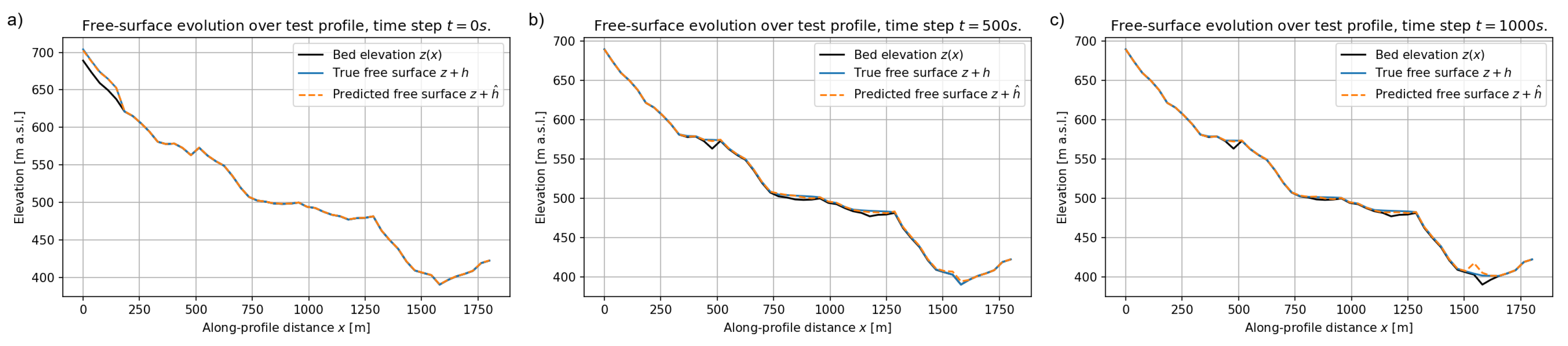
Finally, the corresponding free–surface elevation is shown in Figure 20. Also in this case, the predicted free surface closely follows the reference at all times, demonstrating that the learned operator remains accurate when extrapolated to a new geometric configuration. Figure 20b and Figure 20c highlight the ability of the FNO to reproduce the filling and emptying of local depressions and the gradual downstream migration of the wave crest. The excellent overlap between predicted and reference curves indicates that the coupling between flow depth and bed geometry is robustly captured.
6.6. Inference Performance Comparison
During inference, the FNO model achieved a total execution time of 0.285 seconds for the complete procedure, including the forward pass and denormalization. In comparison, the traditional numerical solver required 10.463 seconds to perform the same task. This demonstrates a performance improvement of more than 36× in favor of the neural operator for inference.
While the solver provides the baseline numerical reference, the FNO enables significantly faster evaluations once trained, making it particularly suitable for scenarios where rapid predictions are essential. All results were obtained using a CPU-based system, but the entire workflow could equally be executed on a machine equipped with a dedicated GPU. In such a configuration, both dataset generation and training times would likely decrease substantially due to higher computational throughput.
However, the proportional advantage observed during inference, where the FNO is dramatically faster than the traditional solver, would remain essentially the same, as this speed-up derives from the intrinsic difference between learned operators and numerical solvers rather than from the underlying hardware.
7. Discussion
The results presented in Section 6 demonstrate that a Fourier Neural Operator trained exclusively on synthetic one-dimensional shallow-water simulations can reproduce debris-flow dynamics with very good accuracy over a broad range of rheological parameters and topographic configurations. In particular, the mean relative error on the flow depth stabilises below approximately on the validation set, while the error on the velocity remains of the order of 10–. For an unseen topographic profile, the relative errors stay within comparable bounds, with error consistent with training errors for both h and u. These findings indicate that the learned operator generalises well within the parameter ranges spanned by the synthetic dataset and can cope with modest extrapolation to new longitudinal geometries.
7.1. Surrogate Performance and Physical Consistency
The spatio–temporal comparisons in Section 6.2–Section 6.4 show that the FNO accurately reconstructs the propagation, deformation, and deposition of the debris surge along the training and validation profiles. The surrogate captures not only the position of the main wave front but also secondary lobes associated with local slope changes. The reconstruction of the free surface over fixed topography is particularly encouraging: for all considered profiles, the predicted free-surface elevation almost coincides with the reference solution throughout the simulation, including the filling of depressions and the final depositional patterns. This suggests that the FNO has learned a physically consistent coupling between the flow depth and the bed geometry, despite being trained purely from data.
As expected, the prediction of the depth-averaged velocity is more challenging than that of the flow depth. The systematic gap – (Figure 7) reflects the fact that exhibits sharper local gradients, sign changes, and transient high-frequency oscillations, especially during the early acceleration phases. A spectral operator such as the FNO, which truncates high-frequency Fourier modes, naturally tends to smooth the smallest velocity fluctuations. Nonetheless, the model still reproduces the main kinematic features of the advancing front and its attenuation in time. For many hazard-related applications, where depth, runout distance, and arrival time are the primary quantities of interest, the achieved accuracy appears fully adequate.
An important qualitative outcome is the absence of overfitting, as indicated by the close tracking between training and validation losses (Figure 5). This is consistent with the operator learning paradigm: the FNO is not fitting individual trajectories but approximating the underlying solution operator of the governing PDEs parametrised by rheological coefficients, initial depth, and bed elevation. The good performance on an unseen profile further supports the interpretation that the network has learned a robust parametric map rather than memorising the training runs.
7.2. Inference Efficiency and Performance Relative to the Numerical Solver
From a practical perspective, the primary advantage of the proposed surrogate lies in its computational efficiency, as demonstrated by the direct comparison between inference times of the trained FNO and the traditional finite-volume solver. During inference, the neural operator required only to generate the full space–time fields and perform the subsequent denormalisation, whereas the numerical solver needed to complete the corresponding simulation. This corresponds to a speed-up exceeding a factor of 36, fully consistent with the qualitative considerations previously discussed and providing empirical confirmation of the transformative potential of operator-learning approaches for rapid scenario evaluation.
It is important to emphasise that these timings were obtained on a CPU-based system. Although migrating the workflow to GPU hardware would accelerate both dataset generation and network training, the relative inference advantage of the FNO over the classical solver would remain essentially unchanged. This disproportion stems not from hardware acceleration but from the intrinsic difference between learned operators, which require only a single forward pass with fixed computational cost, and numerical solvers, whose cost grows with grid resolution, stiffness of the equations, and simulation time. Consequently, even in GPU-accelerated environments, the FNO surrogate would continue to provide dramatic speed-ups, reinforcing its suitability for large ensemble simulations, real-time scenario screening, and operational early-warning systems.
7.3. Implications for Large-Scale and Probabilistic Debris-Flow Hazard Analysis
A more quantitative evaluation of the computational efficiency of the FNO highlights its potential impact on debris-flow hazard assessment. Once trained, the FNO can generate full space–time fields at essentially negligible marginal cost, achieving speed-ups of several orders of magnitude relative to the finite-volume solver. This efficiency becomes particularly valuable when large ensembles of simulations are required for example, to propagate epistemic uncertainty in rheological properties, released volume, or initial saturation conditions. Under these circumstances, computational demands that would be prohibitive for classical solvers become tractable with a trained FNO, enabling Monte Carlo analyses, global sensitivity studies, and near real-time probabilistic hazard mapping.
7.4. Site-Specific Surrogates and Integration with Probabilistic Modelling
Another implication is the feasibility of site-specific surrogates. The synthetic dataset used in this work is tailored to the Morino–Rendinara debris-flow system, with parameter ranges informed by previous back-analyses of the March 2021 event [4]. By focusing on a single catchment, we restrict the parameter and topographic space that the operator must represent, which in turn facilitates high accuracy with a relatively compact network.
This “basin-specific” philosophy aligns with operational practice in engineering hazard assessment, where analyses are typically performed at the scale of an individual valley or infrastructure corridor. In such settings, a dedicated FNO trained on synthetic simulations for that catchment could serve as a lightweight proxy for the original solver, providing instantaneous predictions for early warning systems, scenario screening, or interactive decision-support tools.
The present results also complement recent efforts to use synthetic data for probabilistic debris-flow modelling [22]. In that study, synthetic simulations informed a Bayesian neural network for predicting accumulation volumes, whereas here we use synthetic simulations to train an operator that predicts full space–time fields of depth and velocity. Combining these approaches, for example, using an FNO to generate fast ensembles of fields that are subsequently post-processed by probabilistic models targeting specific impact metrics, could offer a flexible and efficient framework for quantitative risk analysis.
7.5. Limitations and Perspectives for Future Work
Although the proposed framework already demonstrates strong predictive skill and excellent computational efficiency, two main areas of development remain open: extensions of the numerical model and of the underlying physical parametrisation, and expansion and refinement of the dataset towards site-specific and territorial applications.
7.5.1. Extensions of the Physical Model and Numerical Solver
The present study relies on a one-dimensional depth-averaged shallow-water formulation with Voellmy-type basal friction. This setting is well suited for synthetic ensemble generation in confined channels, but it still represents an idealised description of debris-flow dynamics. A more comprehensive numerical framework is envisioned for development, integrating not only additional physical processes, such as internal viscosity, morphodynamic evolution through the Exner equation, spatially varying sediment density, and grain-size segregation and transport, but also a progressive extension of the governing equations and solver architecture from one-dimensional domains to fully two- and three-dimensional geometries. Furthermore, adaptive mesh refinement tailored to local topography and curvature, departing from a uniformly spaced discretization, will be introduced. Moving towards 2D and 3D formulations will allow the model to capture lateral spreading, channel bifurcations, and more complex topographic interactions that cannot be represented in a purely longitudinal framework. The consolidation of these modules, together with an extended suite of verification tests (e.g. analytical benchmarks, uniform-flow equilibrium checks, viscous diffusion tests, and density–Exner consistency evaluations), will enable the creation of richer synthetic datasets that resolve not only flow depth and velocity, but also coupled variations in bed elevation, material composition, and bulk density. These developments will naturally enhance the realism of the training data and substantially expand the operational range of the operator-learning model.
7.5.2. Dataset Expansion, Calibration, and Territorial Scalability
The current surrogate is trained on a finite number of synthetic simulations based on representative profiles of the Morino–Rendinara system. While this ensures physical consistency, the next step towards robust operational performance is to broaden the dataset both geomorphologically and parametrically. This includes incorporating additional field-derived profiles, refining local geomorphological information, and sampling more densely across initial conditions, rheological parameters, and material properties. A more diversified dataset will improve calibration against real landscapes and strengthen generalisation within the basin. Moreover, this strategy provides a scalable pathway for constructing families of site-specific models: by replicating the workflow in other catchments and expanding the corresponding synthetic datasets, it becomes possible to develop territorial Fourier Neural Operators tailored to each zone of interest. Such fast, localised surrogates could then be integrated into early-warning systems, enabling rapid scenario exploration and near real-time hazard assessment at the basin scale.
8. Conclusions
In this work we have developed and evaluated a Fourier Neural Operator (FNO) as a data-driven surrogate for one-dimensional shallow-water debris-flow simulations with Voellmy-type basal friction. FNO is shown to effectively learn the underlying physics of the process, accurately capturing the nonlinear dynamics and wave propagation mechanisms. The surrogate is trained exclusively on synthetic data generated by a validated finite-volume solver applied to longitudinal profiles representative of the Morino–Rendinara debris-flow system. The numerical solver incorporates HLLC and Rusanov fluxes, hydrostatic reconstruction, a robust wet–dry treatment, and diagnostic bulk-density computation, and has been verified against Ritter’s analytical solution for the dam-break problem. On this physically grounded basis, we constructed a large ensemble of synthetic runs by systematically sampling the parameter space of bulk density, initial thickness, and Voellmy friction coefficients over multiple topographic transects.
The resulting FNO learns a mesh-independent operator mapping normalised space–time coordinates, rheological parameters, initial conditions, and bed elevation to the full evolution of flow depth and velocity. On the validation set, the mean relative error on the flow depth stabilises at values below , while the error on velocity typically lies in the range –. For an unseen topographic profile not used during training or validation, the relative errors for both h and u remain in the range – in and norms. The surrogate accurately reproduces the spatio–temporal development of the debris surge, including wave propagation, the formation of secondary lobes, and final deposition, as well as the free-surface elevation over fixed topography. These results indicate that the FNO has effectively learned a physically consistent solution operator for the adopted 1D model.
From an applied perspective, the key advantage of the proposed FNO surrogate is its computational efficiency. Once trained, the model produces full space–time fields at negligible marginal cost, achieving speed-ups of several orders of magnitude with respect to the finite-volume solver. This makes it possible to generate large ensembles of debris-flow scenarios for uncertainty quantification, sensitivity analysis, and probabilistic hazard assessment, which are difficult to realise with traditional solvers alone. In addition, the workflow adopted here is inherently site-specific: it exploits synthetic simulations tailored to the geomorphological and rheological characteristics of the Morino–Rendinara system. This suggests a general strategy for building basin-specific operator learners that act as lightweight, operational proxies for more complex numerical models in early-warning and decision-support contexts.
The study also highlights current limitations and directions for further research. The 1D shallow-water formulation with Voellmy friction provides a computationally convenient but idealised representation of debris-flow dynamics, especially in complex channel networks and fan environments. The velocity field remains more challenging to predict than the flow depth, with systematic underestimation of the sharpest peaks and smoothing of small-scale features. Moreover, the synthetic dataset, while physically informed, samples only a subset of possible geomorphological and rheological conditions.
Future work will focus on three main extensions. First, we plan to expand the numerical model by incorporating additional physical processes, such as internal viscosity, morphodynamic evolution via the Exner equation, spatially varying density, and grain-size segregation, and by extending the solver from one-dimensional to fully two- and three-dimensional geometries. Second, we aim to enlarge and diversify the synthetic datasets through denser sampling of initial and boundary conditions and through the inclusion of additional field-derived profiles, enabling stronger calibration against observations. Third, we envisage the development of territorial families of Fourier Neural Operators trained on multiple catchments, to support near-real-time debris-flow forecasting and scenario exploration at regional scale.
Overall, the present results demonstrate that physics-based synthetic data and operator-learning architectures can be combined into a powerful framework for debris-flow modelling in data-scarce environments. The proposed FNO surrogate bridges the gap between high-fidelity numerical solvers and the computational demands of probabilistic hazard analysis, providing a promising building block for next-generation, fast and flexible debris-flow forecasting systems.
Author Contributions
Conceptualization, M.S. and A.P.; methodology, M.S.; software, M.S. and A.P.; validation, A.P., N.S. and M.M.; formal analysis, M.S.; investigation, M.S., A.P.; resources, A.P., N.S. and M.M.; data curation, M.S. and M.M.; writing—original draft preparation, M.S; writing—review and editing, M.S. and A.P.; visualization, M.S. and A.P; supervision, A.P. and N.S.; project administration, N.S.; funding acquisition, N.S., All authors have read and agreed to the published version of the manuscript.
Funding
This work was supported by the Italian Ministry of University and Research (MUR) under the National Recovery and Resilience Plan (NRRP–Mission 4, Component 2, Investment 1.3–D.D. 1243, 2/8/2022), within the RETURN Extended Partnership–Multi-Risk sciEnce for resilienT commUnities undeR a changiNg climate (Project Code: PE_00000005, CUP: B53C22004020002). The research was conducted as part of the project “LANdslide DAMs (LanDam): characterization, prediction and emergency management of landslide dams”.
Data Availability Statement
The synthetic datasets generated and analyzed during the current study, as well as the training and inference scripts for the Fourier Neural Operator, are available from the corresponding author on reasonable request.
Conflicts of Interest
The authors declare no conflict of interest.
References
- Iverson, R.M. The Physics of Debris Flows. Rev. Geophys. 1997, 35(3), 245–296. [CrossRef]
- Arattano, M.; Franzi, L. Influence of Rheology on Debris-Flow Dynamics. Nat. Hazards Earth Syst. Sci. 2015.
- Pasculli, A.; Cinosi, J.; Turconi, P.; Sciarra, N. Learning Case Study of a Shallow-Water Model to Assess an Early-Warning System for Fast Alpine Muddy-Debris-Flow. Water 2021, 13(6), 750–780. [CrossRef]
- Pasculli, A.; Zito, C.; Sciarra, N.; Mangifesta, M. Back Analysis of a Real Debris Flow, the Morino–Rendinara Test Case (Italy), Using RAMMS Software. Land 2024, 13(12), 2078. [CrossRef]
- Pasculli, A. Viscosity Variability Impact on 2D Laminar and Turbulent Poiseuille Velocity Profiles; Characteristic-Based Split (CBS) Stabilization. In Proceedings of the IEEE Conference, 2018.
- Chung, T.J. Computational Fluid Dynamics, 4th ed.; Cambridge University Press: Cambridge, UK, 2006; p. 1012.
- Audusse, E.; Bouchut, F.; Bristeau, M.-O.; Klein, R.; Perthame, B. A fast and stable well-balanced scheme with hydrostatic reconstruction for shallow water flows. SIAM J. Sci. Comput. 2004, 25, 2050–2065. [CrossRef]
- Gallouët, T.; Hérard, J.-M.; Seguin, N. Some approximate Godunov schemes to compute shallow-water equations with source terms. Comput. Fluids 2003, 32, 479–513.
- Zienkiewicz, O.C.; Taylor, R.L. The Finite Element Method for Solid and Structural Mechanics, 6th ed.; Elsevier: London, UK, 2006; p. 631.
- Paik, J. A high resolution finite volume model for 1D debris flow. J. Hydro-Environ. Res. 2015, 9, 145–155. [CrossRef]
- Pasculli, A.; Minatti, L.; Sciarra, N.; Paris, E. SPH modeling of fast muddy debris flow: Numerical and experimental comparison of certain commonly utilized approaches. Italian Journal of Geosciences 2013, 132(3), 350–365. [CrossRef]
- Bouchut, F. Nonlinear Stability of Finite Volume Methods for Hyperbolic Conservation Laws; Springer: Berlin, Germany, 2004.
- Toro, E.F. Riemann Solvers and Numerical Methods for Fluid Dynamics, 3rd ed.; Springer: Berlin, Germany, 2009.
- Cesca, M.; D’Agostino, V. Comparison Between FLO-2D and RAMMS in Debris-Flow Modelling: A Case Study in the Dolomites. WIT Trans. Eng. Sci. 2008, 60, 197–206.
- Schraml, K.; Thomschitz, B.; McArdell, B.W.; Graf, C.; Kaitna, R. Modeling Debris-Flow Runout Patterns on Two Alpine Fans with Different Dynamic Simulation Models. Nat. Hazards Earth Syst. Sci. 2015, 15, 1483–1492. [CrossRef]
- Mikoš, M.; Bezak, N. Debris Flow Modelling Using RAMMS Model in the Alpine Environment With Focus on the Model Parameters and Main Characteristics. Front. Earth Sci. 2021, 8, 605061. [CrossRef]
- FLO-2D Europe. Condizioni di Vendita e Politica di Rinnovo della Licenza Software FLO-2D PRO. Available online: https://www.flo-2deurope.com.
- WSL Institute for Snow and Avalanche Research SLF. RAMMS::Debrisflow Licensing and Shop Information. Available online: https://ramms.ch.
- Hungr Geotechnical Inc. DAN3D Order and License Types. Available online: https://hungr-geotech.com.
- Kovachki, N.; et al. Neural Operators for Solving Partial Differential Equations. Acta Numer. 2023, 32, 1–153.
- Lu, L.; Jin, P.; Karniadakis, G.E. Learning Nonlinear Operators via DeepONet. Nat. Mach. Intell. 2021, 3, 218–229. [CrossRef]
- Pasculli, A.; Secchi, M.; Mangifesta, M.; Cencetti, C.; Sciarra, N. A Novel Probabilistic Approach for Debris Flow Accumulation Volume Prediction Using Bayesian Neural Networks with Synthetic and Real-World Data. Geosciences 2025, 15(9), 362. [CrossRef]
- Li, Z.; Kovachki, N.; Azizzadenesheli, K.; et al. Fourier Neural Operator for Parametric PDEs. In Proceedings of the International Conference on Learning Representations (ICLR); 2021.
- Li, Z.; et al. Fourier Neural Operator: A Generalist Neural Operator. arXiv 2022, arXiv:2202.09417.
- Kovachki, N.B.; Li, Z.; Liu, B.; et al. Neural Operator: Learning Maps Between Function Spaces. J. Mach. Learn. Res. 2023, 24, 1–97.
- Voellmy, A. Über die Zerstörungskraft von Lawinen. Schweiz. Bauztg. 1955, 73, 159–165.
- Toro, E.F.; Spruce, M.; Speares, W. Restoration of the Contact Surface in the HLL Riemann Solver. Shock Waves 1994, 4, 25–34. [CrossRef]
- Rusanov, V.V. Calculation of Interaction of Non-Steady Shock Waves with Obstacles. USSR Comput. Math. Math. Phys. 1961, 1, 304–320.
- Minatti, L.; Pasculli, A. Dam break Smoothed Particle Hydrodynamic modeling based on Riemann solvers. In Advances in Fluid Mechanics VIII, WIT Transactions on Engineering Sciences; WIT Press: 2010; Vol. 69, 145–156.
- Ritter, A. Die Fortpflanzung der Wasserwellen. Zeitschrift des Vereins Deutscher Ingenieure 1892, 36, 947–954.
- Kashtalyan, K.; et al. Machine-Learning Surrogates for Geophysical Flows: A Review. Earth-Sci. Rev. 2023, 238, 104345.
- Bi, X.; Li, Z.; Azizzadenesheli, K.; Anandkumar, A. Physics-Informed Fourier Neural Operators for Learning Shallow Water Equations. arXiv 2022, arXiv:2205.01436.
- Shen, Z.; et al. Fourier Neural Operators for Fast Flood and Hydrodynamic Modelling. Adv. Water Resour. 2024, 181, 104566.
- Raissi, M.; Perdikaris, P.; Karniadakis, G.E. Physics-Informed Neural Networks: A Deep Learning Framework for Solving Forward and Inverse Problems Involving Nonlinear PDEs. J. Comput. Phys. 2019, 378, 686–707. [CrossRef]
- Holl, P.; Thuerey, N.; et al. Learning to Simulate Complex Physics with Graph Networks. In Proceedings of the 37th International Conference on Machine Learning (ICML); 2020.
- Mergili, M.; Fischer, J.-T.; Krenn, J.; Pudasaini, S.P. r.avaflow v1, an Advanced Open-Source Computational Framework for the Propagation and Interaction of Two-Phase Mass Flows. Geosci. Model Dev. 2017, 10, 553–569. [CrossRef]
Figure 1.
Dam-break test with HLLC flux. Water-depth profiles at s for . The dashed line corresponds to Ritter’s analytical solution.
Figure 1.
Dam-break test with HLLC flux. Water-depth profiles at s for . The dashed line corresponds to Ritter’s analytical solution.
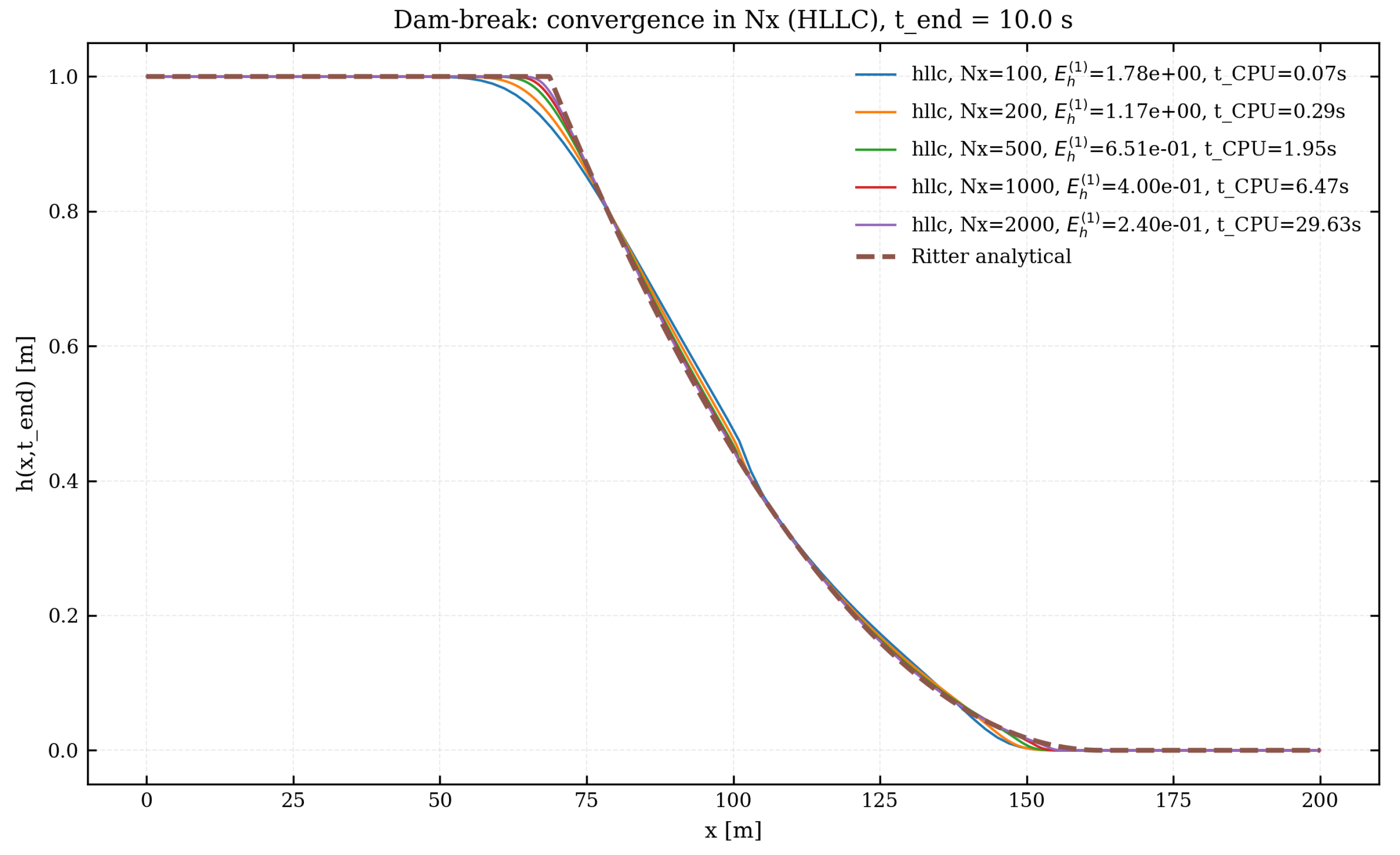
Figure 2.
Dam-break test with Rusanov flux. Water-depth profiles at s. The dashed line corresponds to Ritter’s analytical solution.
Figure 2.
Dam-break test with Rusanov flux. Water-depth profiles at s. The dashed line corresponds to Ritter’s analytical solution.
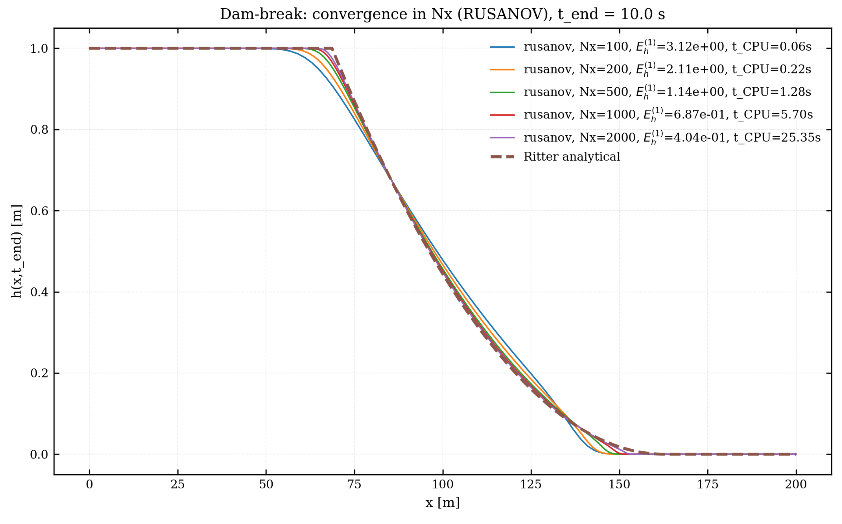
Figure 3.
Locations of the eight topographic profiles used in the numerical simulations, traced over the orthophoto and DEM of the Morino–Rendinara debris–flow system. The blu profile (profile 1) represent the Rio Sonno channel. The colour code identifies the eight transects. Black dots mark the profile endpoints, and the north orientation is indicated on the right.
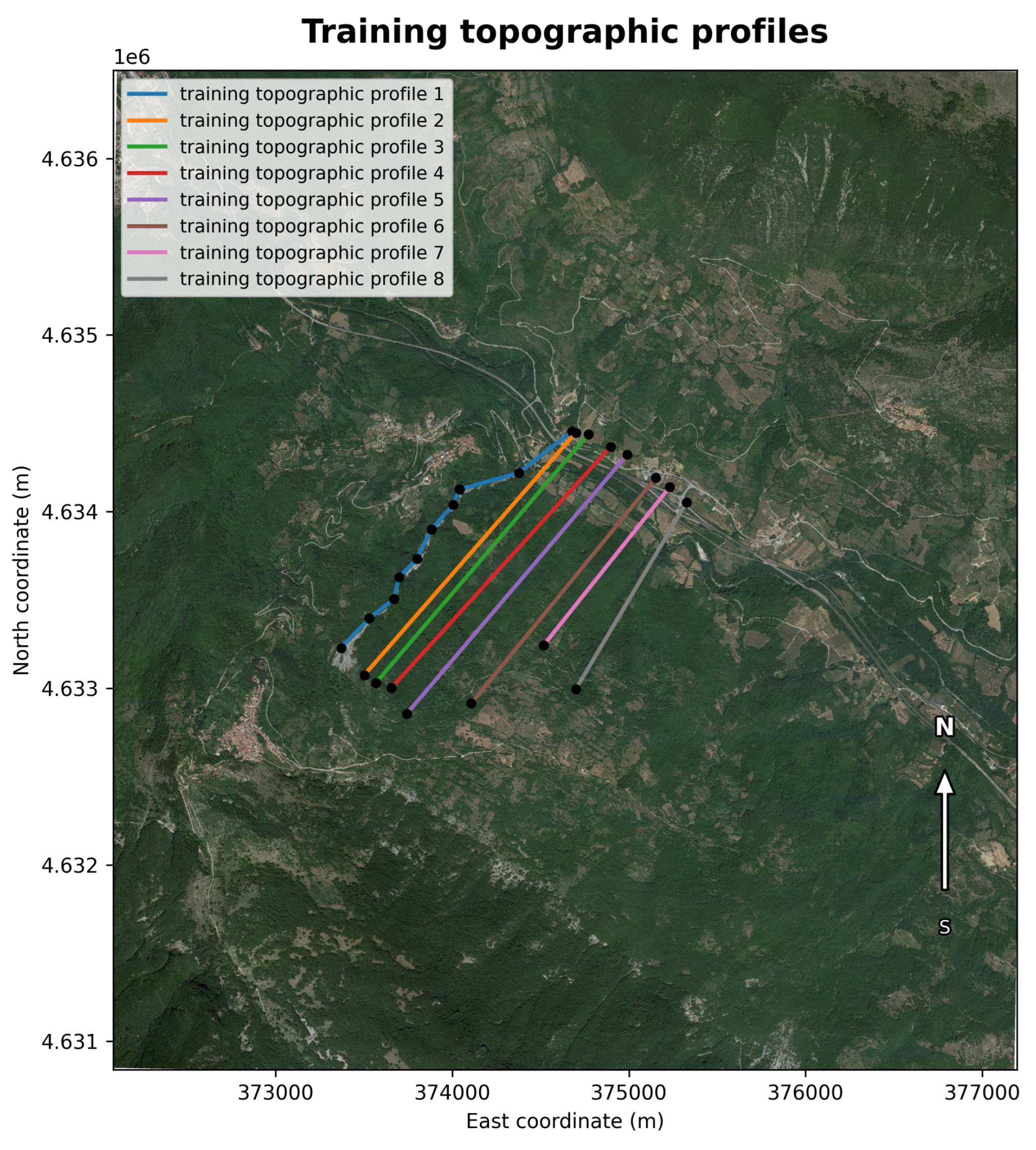
Figure 4.
(a) Architecture of the Fourier Neural Operator: the input field is lifted to a latent representation via P, propagated through T Fourier layers, and projected back to obtain the output through Q [23]. (b) Internal structure of a Fourier layer: Fourier transform , learned spectral weights R, inverse transform , pointwise linear map W, and activation . The spectral pathway models nonlocal interactions while W accounts for local effects [23].
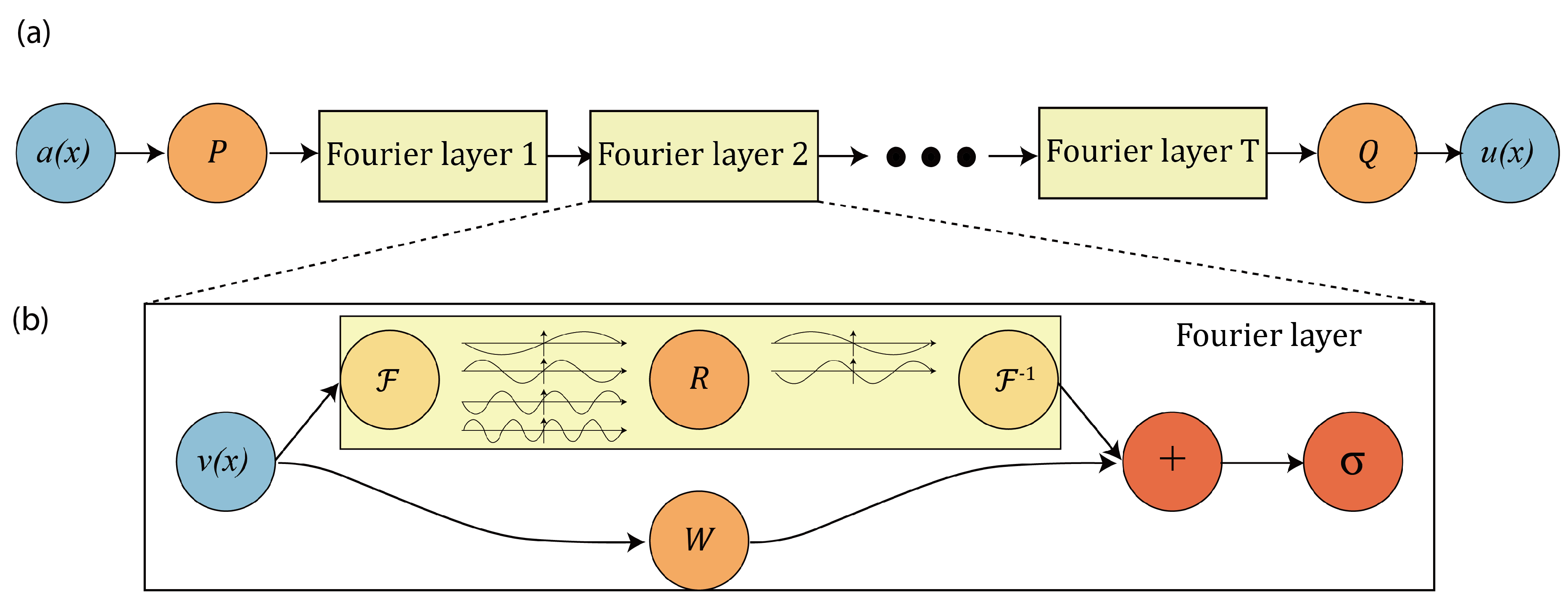
Figure 5.
Total training and validation loss as a function of the epoch during FNO optimisation.
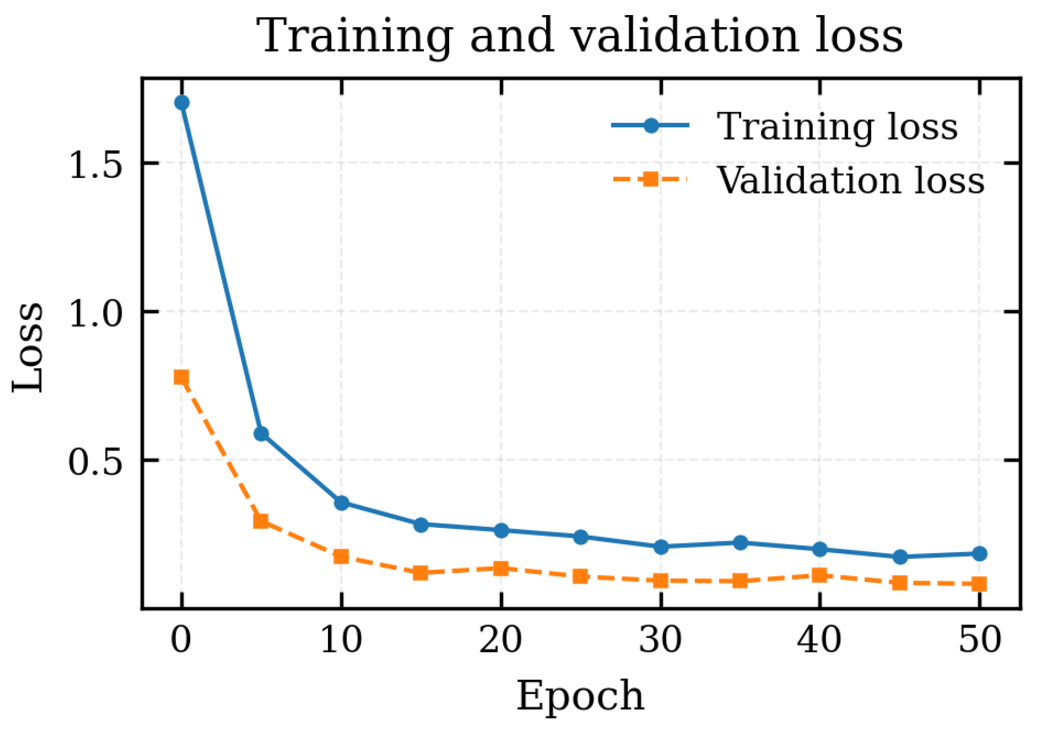
Figure 6.
Relative validation errors for flow depth h and velocity u as a function of the epoch.
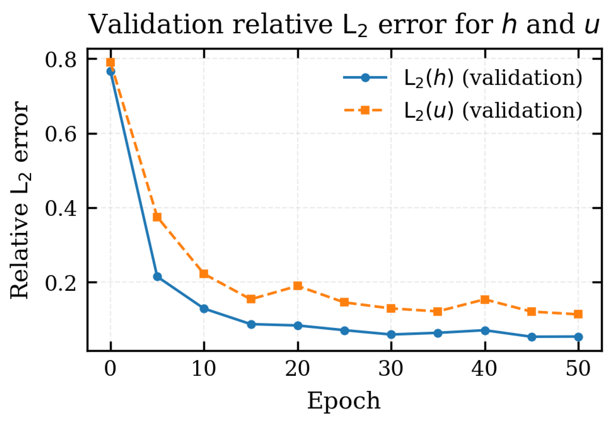
Figure 7.
Ratio between the relative validation errors on velocity and depth, , as a function of the epoch.
Figure 7.
Ratio between the relative validation errors on velocity and depth, , as a function of the epoch.
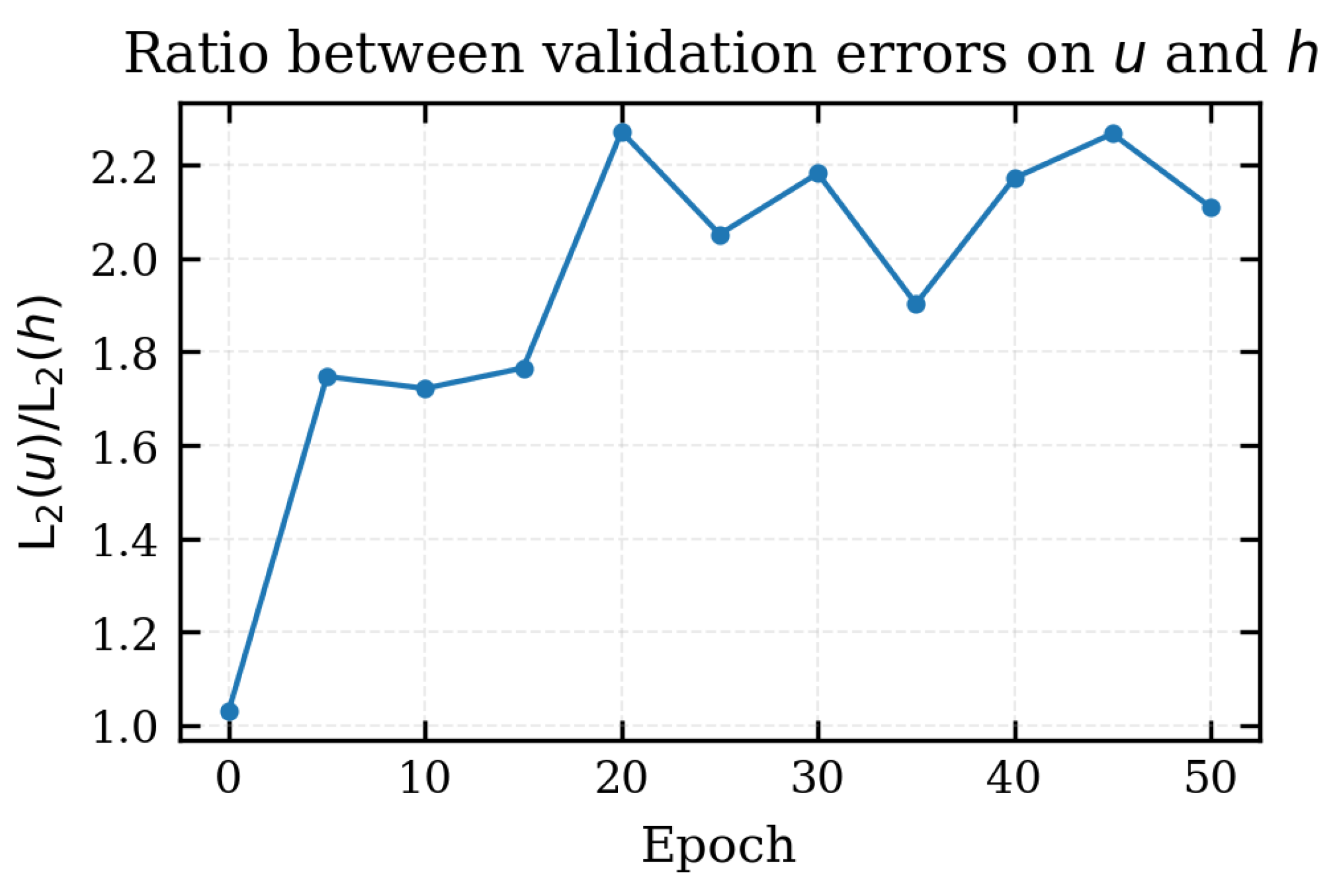
Figure 8.
Flow depth along validation profile ID=04 at (a) s, (b) s, and (c) s. Blue solid lines: reference numerical solution ; orange dashed lines: FNO prediction .
Figure 8.
Flow depth along validation profile ID=04 at (a) s, (b) s, and (c) s. Blue solid lines: reference numerical solution ; orange dashed lines: FNO prediction .
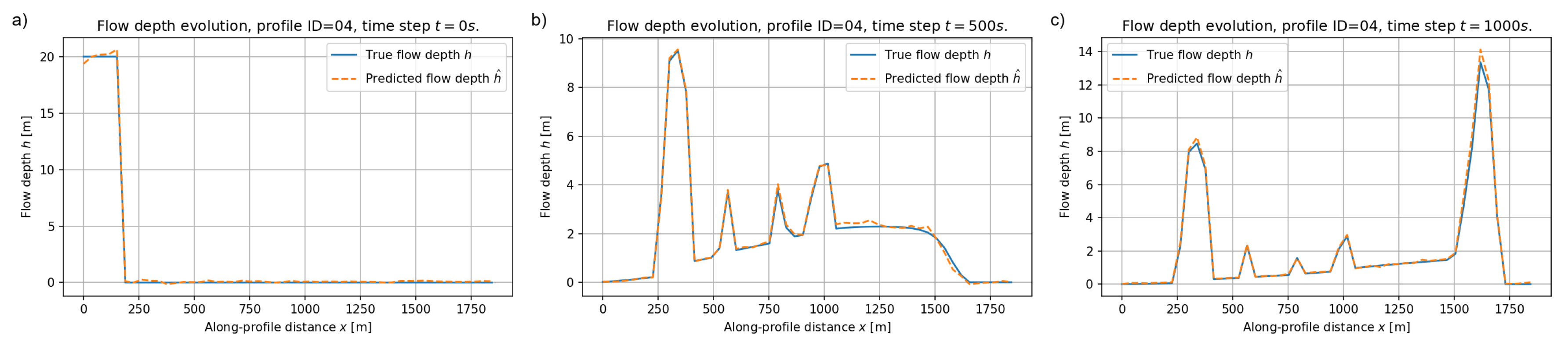
Figure 9.
Flow depth along validation profile ID=05 at (a) s, (b) s, and (c) s. Blue solid lines: reference depth ; orange dashed lines: predicted depth .
Figure 9.
Flow depth along validation profile ID=05 at (a) s, (b) s, and (c) s. Blue solid lines: reference depth ; orange dashed lines: predicted depth .
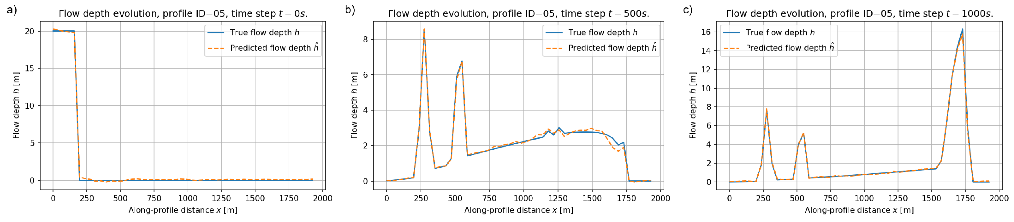
Figure 10.
Flow depth along validation profile ID=08 at (a) s, (b) s, and (c) s. Blue solid lines: reference depth ; orange dashed lines: predicted depth .
Figure 10.
Flow depth along validation profile ID=08 at (a) s, (b) s, and (c) s. Blue solid lines: reference depth ; orange dashed lines: predicted depth .
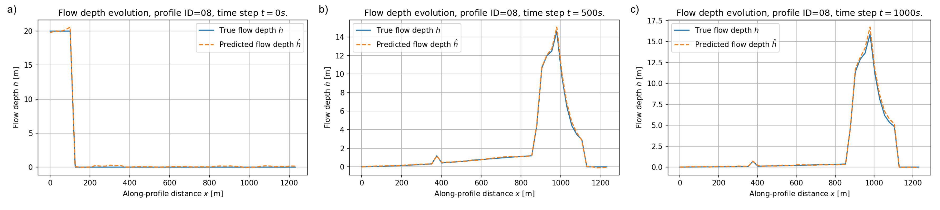
Figure 11.
Depth–averaged velocity along validation profile ID=04 at (a) s, (b) s, and (c) s. Blue solid lines: reference velocity ; orange dashed lines: FNO prediction .
Figure 11.
Depth–averaged velocity along validation profile ID=04 at (a) s, (b) s, and (c) s. Blue solid lines: reference velocity ; orange dashed lines: FNO prediction .
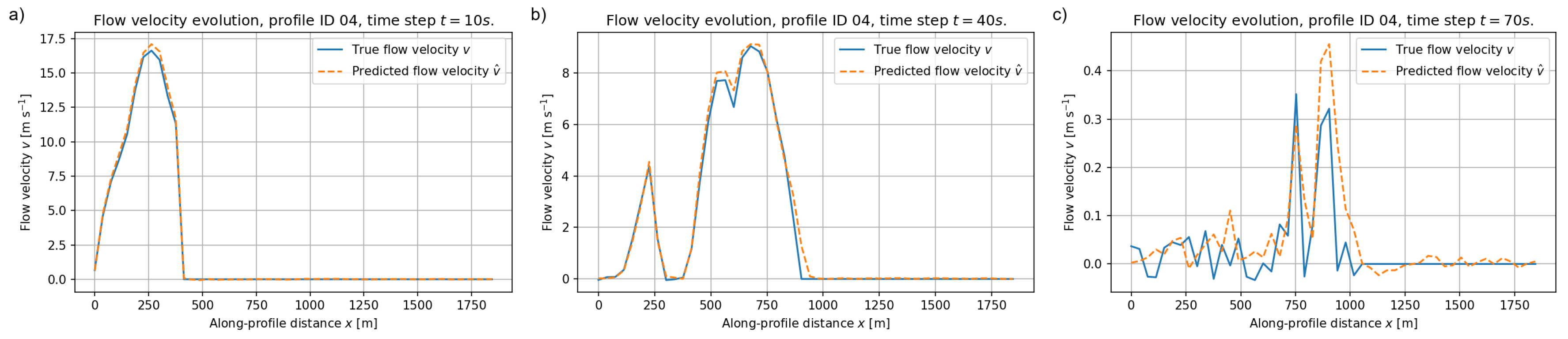
Figure 12.
Depth–averaged velocity along validation profile ID=05 at (a) s, (b) s, and (c) s. Blue solid lines: reference solution ; orange dashed lines: FNO prediction .
Figure 12.
Depth–averaged velocity along validation profile ID=05 at (a) s, (b) s, and (c) s. Blue solid lines: reference solution ; orange dashed lines: FNO prediction .
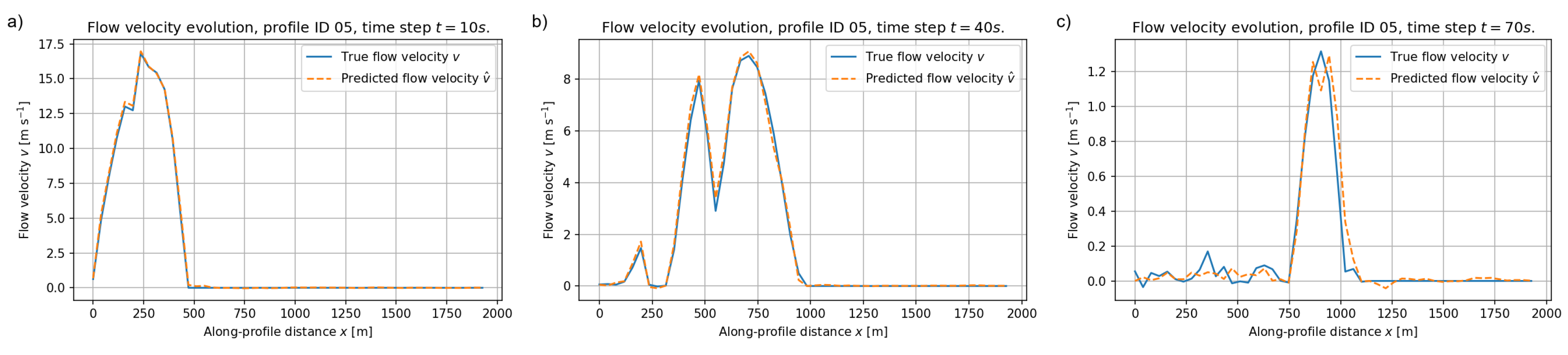
Figure 13.
Depth–averaged velocity along validation profile ID=08 at (a) s, (b) s, and (c) s. Blue solid lines: reference velocity ; orange dashed lines: FNO prediction .
Figure 13.
Depth–averaged velocity along validation profile ID=08 at (a) s, (b) s, and (c) s. Blue solid lines: reference velocity ; orange dashed lines: FNO prediction .
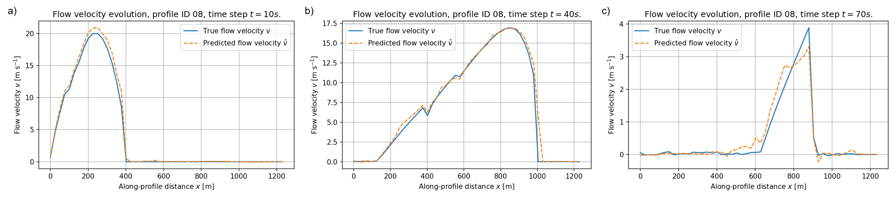
Figure 14.
Free surface over topography for validation profile ID=04 at (a) s, (b) s, and (c) s. Black line: bed elevation ; blue solid line: reference free surface ; orange dashed line: predicted free surface .
Figure 14.
Free surface over topography for validation profile ID=04 at (a) s, (b) s, and (c) s. Black line: bed elevation ; blue solid line: reference free surface ; orange dashed line: predicted free surface .
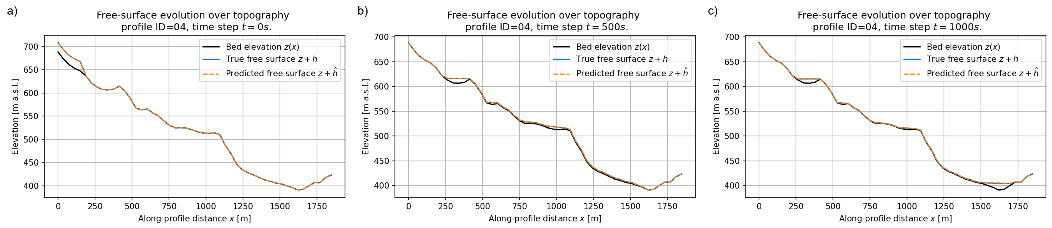
Figure 15.
Free surface over topography for validation profile ID=05 at (a) s, (b) s, and (c) s. Black line: bed elevation ; blue solid line: reference free surface ; orange dashed line: predicted free surface .
Figure 15.
Free surface over topography for validation profile ID=05 at (a) s, (b) s, and (c) s. Black line: bed elevation ; blue solid line: reference free surface ; orange dashed line: predicted free surface .
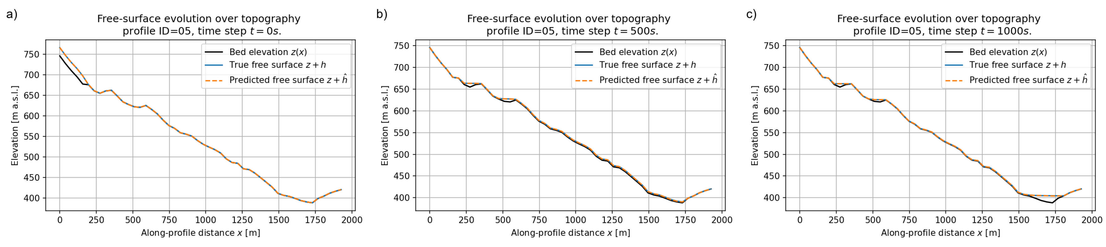
Figure 16.
Free surface over topography for validation profile ID=08 at (a) s, (b) s, and (c) s. Black line: bed elevation ; blue solid line: reference free surface ; orange dashed line: predicted free surface .
Figure 16.
Free surface over topography for validation profile ID=08 at (a) s, (b) s, and (c) s. Black line: bed elevation ; blue solid line: reference free surface ; orange dashed line: predicted free surface .
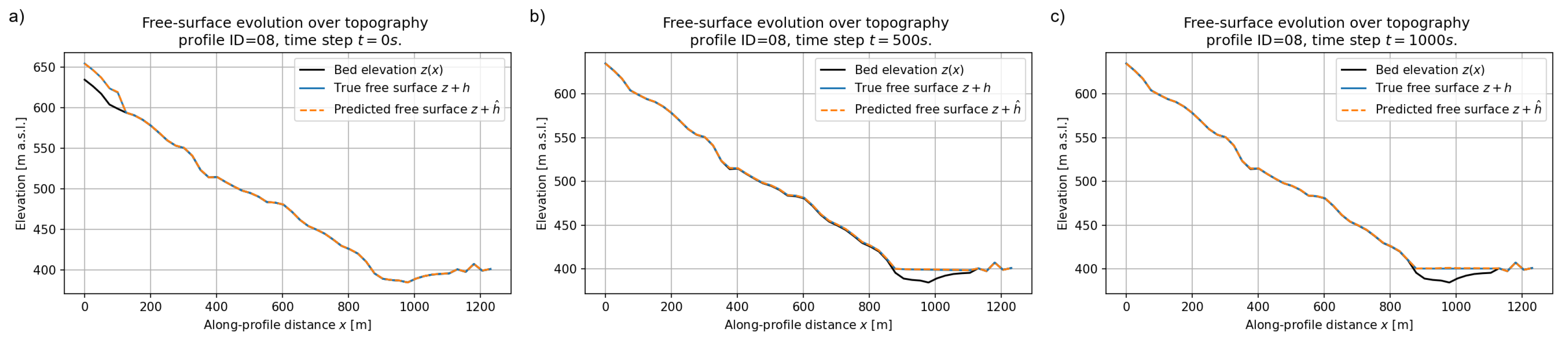
Figure 17.
Location of the unseen test profile (blue line) within the study area, plotted over the orthophoto and DEM.
Figure 17.
Location of the unseen test profile (blue line) within the study area, plotted over the orthophoto and DEM.
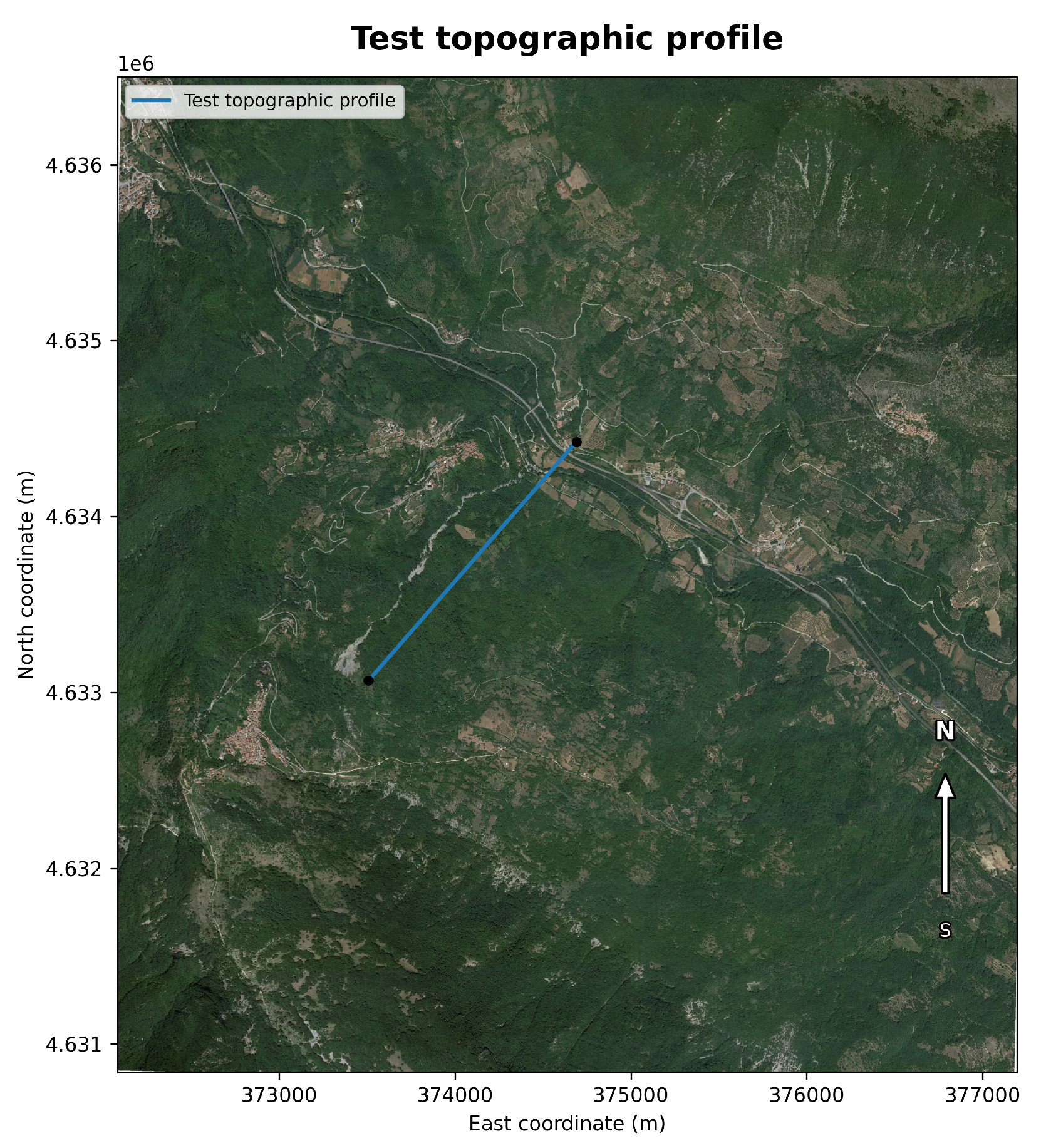
Figure 18.
Flow depth along the unseen test profile at (a) s, (b) s, and (c) s. Blue lines: reference depth ; orange dashed lines: FNO prediction .
Figure 18.
Flow depth along the unseen test profile at (a) s, (b) s, and (c) s. Blue lines: reference depth ; orange dashed lines: FNO prediction .
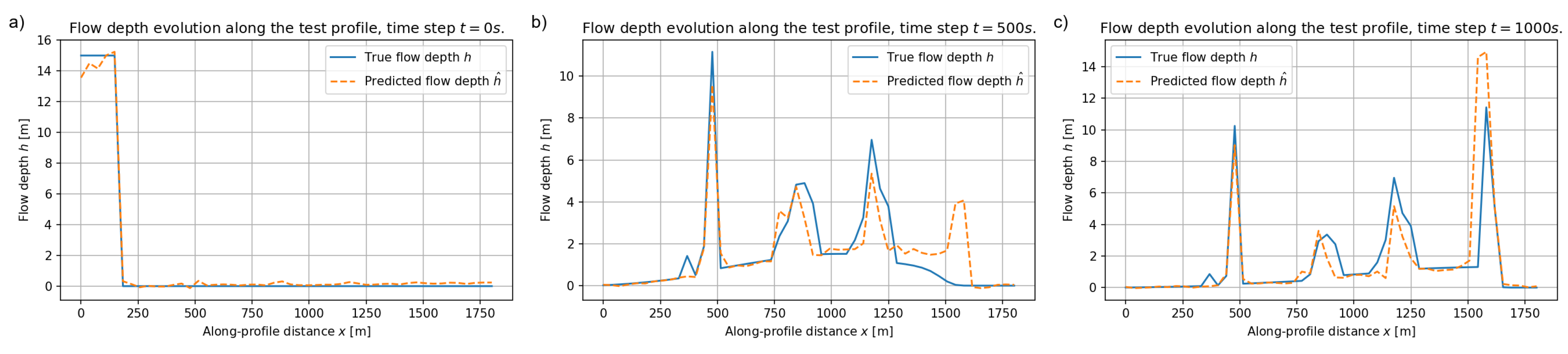
Figure 19.
Depth–averaged velocity along the unseen test profile at (a) s, (b) s, and (c) s. Blue lines: reference velocity ; orange dashed lines: prediction .
Figure 19.
Depth–averaged velocity along the unseen test profile at (a) s, (b) s, and (c) s. Blue lines: reference velocity ; orange dashed lines: prediction .
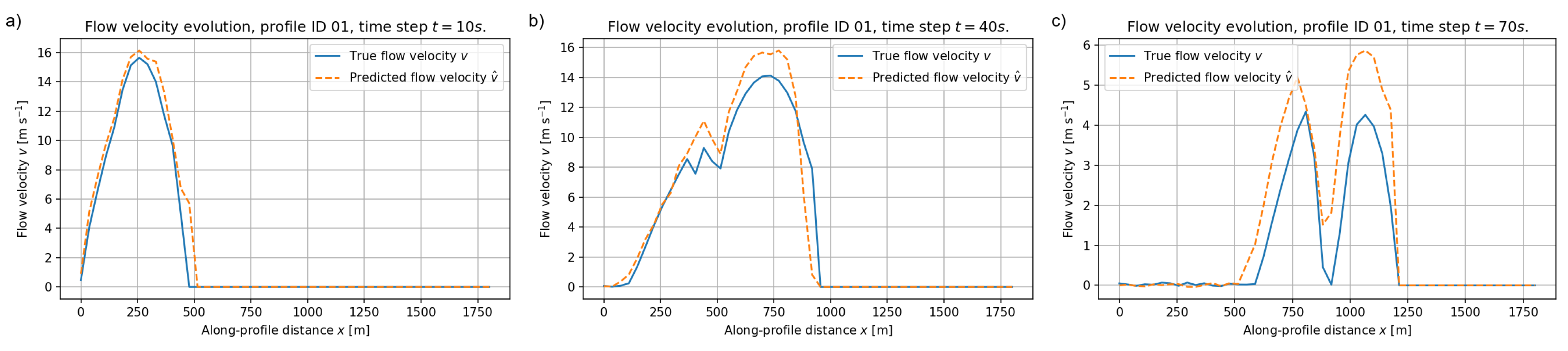
Figure 20.
Free surface over the unseen test profile at (a) s, (b) s, and (c) s. Black lines: bed elevation ; blue lines: reference free surface ; orange dashed lines: predicted free surface .
Figure 20.
Free surface over the unseen test profile at (a) s, (b) s, and (c) s. Black lines: bed elevation ; blue lines: reference free surface ; orange dashed lines: predicted free surface .
Disclaimer/Publisher’s Note: The statements, opinions and data contained in all publications are solely those of the individual author(s) and contributor(s) and not of MDPI and/or the editor(s). MDPI and/or the editor(s) disclaim responsibility for any injury to people or property resulting from any ideas, methods, instructions or products referred to in the content. |
© 2025 by the authors. Licensee MDPI, Basel, Switzerland. This article is an open access article distributed under the terms and conditions of the Creative Commons Attribution (CC BY) license (http://creativecommons.org/licenses/by/4.0/).
Copyright: This open access article is published under a Creative Commons CC BY 4.0 license, which permit the free download, distribution, and reuse, provided that the author and preprint are cited in any reuse.


