Submitted:
12 December 2025
Posted:
16 December 2025
You are already at the latest version
Abstract
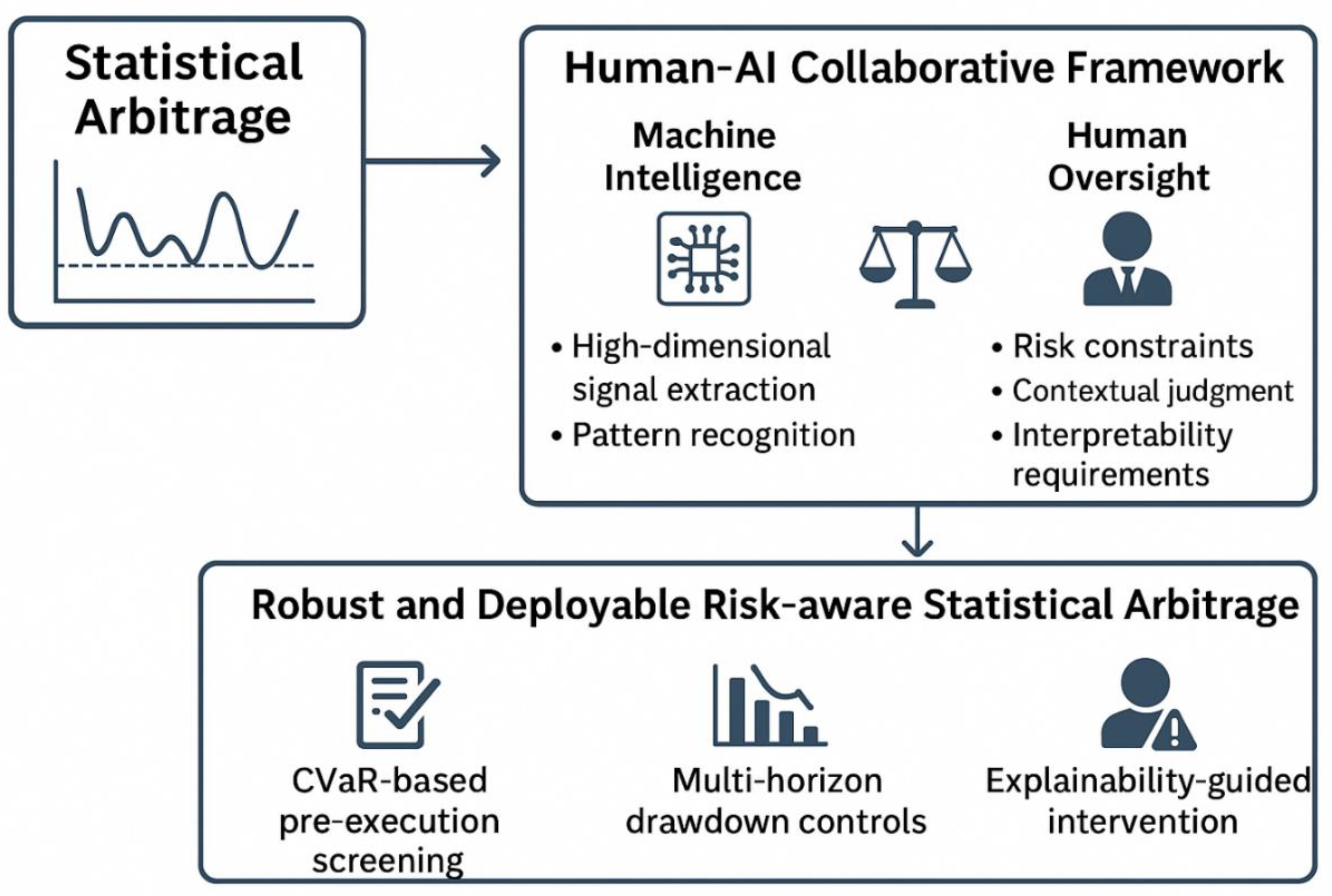
This paper presents a structured synthesis of the statistical arbitrage literature, tracing the evolution of the field from classical mean-reversion and cointegration frameworks to contemporary machine learning and reinforcement learning architectures. Through a comparative analysis of prior empirical studies across equity, ETF, and cryptocurrency markets, the paper finds that although rising market efficiency and structural complexity have weakened the persistence of traditional signals, statistical arbitrage retains meaningful potential when supported by adaptive modeling and robust risk management. To address challenges related to tail-risk exposure, model fragility, and declining interpretability, this study proposes a human–AI collaborative execution framework. In this system, machine intelligence focuses on high-dimensional signal extraction and pattern recognition, while human oversight enforces risk constraints, contextual judgment, and interpretability requirements. This complementary structure is operationalized through CVaR-based pre-execution screening, multi-horizon drawdown controls, and explanability-guided intervention, forming a resilient and practically deployable architecture for risk-aware statistical arbitrage.
Keywords:
statistical arbitrage
; pair trading
; risk-adjusted performance
; mean reversion
; machine learning
; CVaR
; model interpretability
1. Introduction
According to the Efficient Market Hypothesis (EMH), asset prices fully incorporate available information, leaving little room for persistent abnormal returns (Fama, 1970). Nonetheless, decades of empirical evidence on statistical arbitrage—especially pair trading based on cointegration and mean-reverting spreads—demonstrate that temporary pricing deviations can and do emerge in practice (Gatev et al., 2006). These deviations, although often short-lived, form the conceptual foundation of systematic arbitrage strategies designed to exploit relative mispricing across related assets.
Over time, however, fundamental changes in market structure—such as the proliferation of algorithmic trading, the rise of cryptocurrency markets and the increasing complexity of global financial networks—have challenged the assumptions underlying traditional linear and parametric models. In response, researchers and practitioners have progressively adopted machine learning and deep learning techniques, including LSTM and reinforcement learning, with a focus on tail risk control (e.g., CVaR) and model interpretability, to capture nonlinear patterns, adapt to regime shifts and scale strategies across large universes of assets. While these methods often enhance predictive power, they simultaneously introduce new vulnerabilities, including overfitting, reduced transparency and heightened exposure to extreme market events.
This paper explores the evolution of statistical arbitrage through four interconnected dimensions: theoretical origins, methodological transformation, cross-market applications and emerging integration with human judgement. Rather than positioning machine learning as a wholesale replacement for classical approaches, we argue that a hybrid, human-AI framework offers a more balanced and resilient path forward. By synthesising existing methods, highlighting their respective strengths and limitations, and placing explicit emphasis on risk-adjusted performance and interpretability, this study aims to inform the development of more robust and responsible algorithmic trading systems.
In light of the above structural framework, this study is designed to address several core research questions that guide the subsequent analysis. (1) How can machine learning-driven statistical arbitrage frameworks overcome the diminishing profitability, linear constraints, and structural fragility inherent in traditional mean-reversion models? (2) How do AI-empowered statistical arbitrage strategies perform across different financial markets—such as equities, foreign exchange, cryptocurrencies, ETFs and derivatives—under heterogeneous market microstructures and volatility regimes? (3) In what specific ways can human expertise complement artificial intelligence to enhance the robustness, interpretability, and regulatory compliance of AI-based statistical arbitrage systems? By systematically exploring these questions, the paper establishes a coherent analytical pathway that bridges theoretical evolution and methodological innovation, thereby laying the foundation for the contributions summarized below.
Overall, this study contributes to the literature by (1) highlighting the evolution of statistical arbitrage from a linear mean-reversion (cointegration) paradigm to a multifaceted, data-driven framework capable of capturing more complex market dynamics; (2) demonstrating that while traditional strategies exhibit diminishing returns due to increasing market efficiency and transaction costs, AI-based approaches show stronger potential, particularly in volatile and less mature markets such as cryptocurrencies; (3) emphasizing that the effective implementation of modern statistical arbitrage requires a multi-stage workflow involving robust data preprocessing, dynamic risk management, and careful consideration of market microstructure, frictions, and regulatory constraints; and (4) proposing a human-AI collaborative statistical arbitrage framework in which artificial intelligence models are complemented by human expertise to enhance stability, regulatory compliance, and decision transparency.
2. Theoretical Foundations and Core Issues
In its traditional definition, statistical arbitrage was initially defined as an arbitrage strategy based on quantitative methods and statistical models. Its core logic lies in exploiting the mean-reversion characteristics of price series to capture temporary mispricing (Gatev et al., 2006). This traditional definition of statistical arbitrage is grounded in the premise of limited failures of the weak-form efficient market hypothesis—markets may deviate from fundamental-based pricing in the short term but will revert to the mean over the long term. Its typical methodology can be broadly summarized as the “mean reversion-cointegration-pair trading” paradigm: First, cointegration tests are used to identify pairs of stocks exhibiting long-term equilibrium relationships. If the spread or ratio between them deviates from historical equilibrium levels, pair trades are executed (establishing a long position in the undervalued asset and a short position in the overvalued asset, thereby capturing low-risk or even risk-free arbitrage profits when prices revert) (Elliott et al., 2005; R. F. Engle & Granger, 1987). Formally, the simplest two-asset pair trade can be expressed as constructing a spread, (or logarithmic spread), assuming this spread follows a stationary mean-reverting process. In the continuous limit, it is often modeled as an Ornstein-Uhlenbeck process:
The speed of mean reversion κ > 0 ensures the recoverability of deviations, thereby generating “realizable arbitrage signals.” This modeling approach forms the theoretical foundation of classical statistical arbitrage, focusing on mean reversion and adopted by a series of modeling studies. Traditional statistical arbitrage models primarily rely on linear econometric methods and stationarity tests, emphasizing the dynamic process of market imbalance followed by reversion to mean. This provided the foundational framework for early quantitative hedge fund strategies.
With the continuous development of modern markets, market structures have become increasingly complex, and investor behavior has grown more diverse. Consequently, research and practice in statistical arbitrage have gradually moved beyond the classical paradigm of “mean reversion-cointegration-pair trading,” giving rise to several modern extensions. The original statistical arbitrage was built upon the assumption of highly rational investors and did not overemphasize the analysis of human psychology. Contemporary scholars, however, have introduced behavioral finance perspectives into traditional theories, addressing the “human blind spots” overlooked by conventional finance. Relevant researchers argue that investors’ cognitive biases and bounded rationality may lead to the alternating presence of momentum and reversal effects (Jegadeesh & Titman, 1993). Within this framework, statistical arbitrage no longer relies solely on mean reversion assumptions but simultaneously accounts for trend persistence, forming a dual mechanism of “mean reversion-momentum.” Furthermore, modern researchers emphasize the significant impact of market frictions (transaction costs, liquidity constraints, short-selling restrictions, etc.) on the feasibility of statistical arbitrage (Avellaneda & Lee, 2010; Jarrow et al., 2012). Unlike the frictionless markets assumed in earlier models, modern statistical arbitrage models often require dynamic optimization and risk control methods to comprehensively account for execution delays, impact costs, and leverage constraints, ensuring the strategy’s effectiveness in practice. Furthermore, with the rapid growth of computational power in this information era, statistical arbitrage has progressively integrated high-frequency trading and machine learning techniques into its practical strategies.
2.1. The Economic Significance of Statistical Arbitrage
Beyond its usage in generating profits in financial markets, the existence of statistical arbitrage also has a profound influence in the study of economic. According to Fama’s classic definition (1970), the EMH posits that financial markets accurately and unbiasedly reflect all available information, which means systematic excess returns is actually unattainable. However, empirical evidence from statistical arbitrage clearly demonstrates that quantitative methods can consistently identify and exploit mispricing across assets, yielding substantial arbitrage profits (Balladares et al., 2021; Hogan et al., 2004). This implies that market price movements are not entirely random but exhibit short-term and medium-term deviations and predictability, directly challenging the logical premises of weak-form and even semi-strong-form market efficiency. More importantly, statistical arbitrage constitutes a systematic strategy that provides repeatable and testable evidence of arbitrage profitability, thereby constituting a methodological rebuttal to the Efficient Market Hypothesis. In short, statistical arbitrage uses quantitative models to expose systemic market inefficiencies rather than isolated anomalies. This not only challenges the tradtional foundations of the theory of perfectly efficient markets but also provides rich empirical evidence for the subsequent rise of behavioral finance and market friction theories. From an economic perspective, the significance of statistical arbitrage lies in revealing the actual existence of information asymmetry and investor bounded rationality in financial markets, thereby driving a re-examination and revision of market efficiency theory.
2.2. Key Issues and Controversies
In the preceding discussion, statistical arbitrage has been defined as a systematic trading approach based on the mean reversion hypothesis, capturing pricing deviations with pair trading as its typical strategy. On the other hand, its scope has expanded beyond the traditional “spread reversion framework.” In modern extensions, behavioral finance and market frictions have been incorporated, which emphasizes the roles of investor bounded rationality, liquidity friction, and risk compensation. However, regardless of the perspective taken, statistical arbitrage faces controversies both academically and in practical application.
First is the persistence of mean reversion: As the core of traditional statistical arbitrage theory, mean reversion does not consistently hold across all market conditions and time horizons in practice. In the short term, delayed price reactions and overshooting can create arbitrage opportunities (Jegadeesh & Titman, 1993). However, over the long term, long-term memory and structural risk may distort or even delay the mean reversion process. Prices may remain elevated for extended periods or fail to converge toward the mean, rendering the strategy ineffective (Hong & Stein, 2007; Ramos-Requena et al., 2020; Serrano & Hoesli, 2012). This implies that: Mean reversion may not exist in the long run, it is just a localized, temporary phenomenon. Whether statistical arbitrage can sustain itself through such strategies in the long run remains questionable to us.
Second, in terms of return effectiveness: As modern market efficiency advances and investors grow more sophisticated, arbitrage opportunities have diminished steadily year on year. Traditional statistical arbitrage strategies, such as simple pair trading, have shown clear signs of weakness in practical application, with their returns converging gradually over time. In their systematic tests of pair trading, Do and Faff (2010) found that the performance of many strategies is highly dependent on the sample period and market conditions in place, this makes it difficult to achieve robust returns across different time periods. Stephenson et al. (2010) further argued that simple pair trades struggle to sustain stable and significant returns in the current market environment. Therefore, more innovation should be found to fuel statistical arbitrage.
3. Methodological Evolution: From Classical Models to Artificial Intelligence
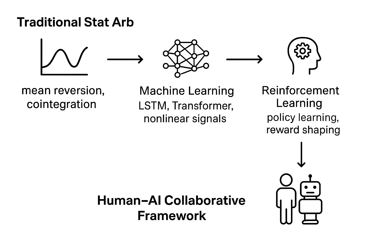
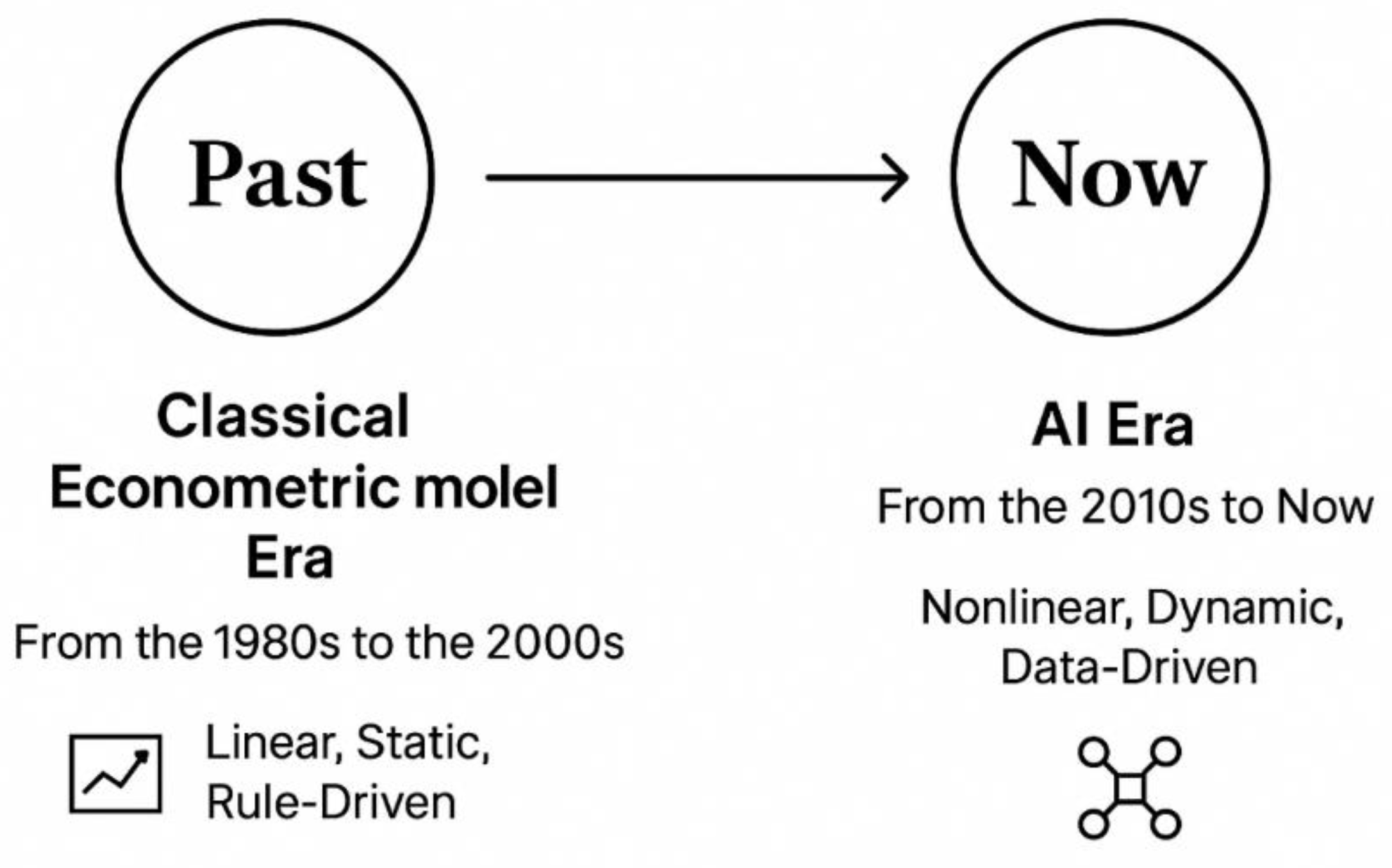
The previous sections thoroughly discussed the theoretical basis and core contradictions of statistical arbitrage. In the long run, these characteristics remain almost unchanged. In recent years, they have changed little and evolved slowly. On the contrary, the iterative development of statistical arbitrage methods is closely related to the transformation of the financial market structure, the breakthrough of measurement technology and the progress of computing power. In this era of rapid artificial intelligence and information technology, its evolution is rapid and change. From a comprehensive academic and practical perspective, this evolution can be clearly divided into two main stages: the era of classical econometric models (1980s-2000s) and the era of artificial intelligence (2010s-now). The era of classical econometric models is based on linear hypotheses and structured modeling frameworks, while the era of artificial intelligence broke the previous technical boundaries through large-scale multi-dimensional data-driven nonlinear learning. These two eras have jointly promoted the return of statistical arbitrage from simple computation to a multi-dimensional intelligent decision-making model.
Exhibits 1.
The evolution of statistical arbitrage across eras.
2.3. Statistical Arbitrage in the Era of Classical Econometric Model
The core logic of statistical arbitrage in the era of classical econometric models can be generally summarized as: “Identify stable statistical relationships between assets, Model the mean-reversion process of spreads, Design arbitrage signal triggering mechanisms.” Its technical framework centers primarily on these three key breakthroughs. To transform statistical arbitrage from the theoretical premise of “market imperfect efficiency” into an executable quantitative trading strategy, one must follow six progressive steps: Data Preprocessing, Statistical Relationship Identification, Factor and Dimension Optimization, Dynamic Forecasting and Signal Capture, Volatility and Risk Control, and Deepening Multivariate Dependencies. Through ongoing refinement via methodologies such as econometrics and mathematics, the strategy ultimately satisfies three core criteria: statistical significance, out-of-sample robustness, and adaptability to market friction. In the sections that follow, these six steps will be deconstructed in sequence in line with technical logic, elaborating on how robust technical methods boost the rationality and effectiveness of quantitative strategies—thereby facilitating more straightforward implementation and enabling the achievement of meaningful returns.
The rise of classic statistical arbitrage models was no accident, but rather the combined result of the “quantitative revolution” and rapid breakthroughs in econometrics during the 1970s. At that time, the academic groundwork for statistical arbitrage was primarily laid in econometrics laboratories at U.S. universities (led by institutions like MIT and UC San Diego), while its practical application took root in quantitative hedge funds on Wall Street. The U.S. stock market had already developed relatively sophisticated trading mechanisms, yet investor sophistication remained relatively low (primarily relying on fundamental analysis). Coupled with the rapid advancement of computing power, these factors provided crucial conditions for the successful implementation of statistical arbitrage. The development of classic statistical arbitrage models during this period was primarily established by leading econometricians, such as 2003 Nobel laureate Robert F. Engle (University of California, San Diego) and Clive W.J. Granger (University of East Anglia, UK, long-term researcher in the US), along with Danish econometrician Søren Johansen (University of Copenhagen, closely collaborating with US academia). Their research laid the cornerstone for the traditional econometric era.
2.3.1. Data Preprocessing
Data preprocessing is a foundational step in constructing statistical arbitrage strategies, as it addresses critical data quality issues. The priority of data preprocessing lies in systematically addressing the four critical inherent flaws in financial market data: non-stationarity, outlier interference, dimensional heterogeneity, and high-frequency noise pollution. Failing to resolve these flaws will significantly impact the subsequent construction of investment strategies. Therefore, data preprocessing must adhere to principles of statistical rigor and financial market applicability, enhancing data quality through multiple steps. Key methods include data cleaning, stationarity adjustment, normalization, and noise reduction. Collectively, these ensure data authenticity, stability, and signal-to-noise ratio, laying a solid foundation for statistical arbitrage model construction.
Data Cleaning: During the process of collecting financial data, outliers may easily occur due to reasons like liquidity gaps, extreme investor trading behavior, or trading software malfunctions. Missing values may arise from individual stock suspensions or data interface interruptions. Data cleaning adheres to the principle of accurately identifying anomalies and reasonably filling missing values to prevent subsequent statistical models from being compromised by data issues. The most common method for identifying outliers is Median Absolute Deviation (MAD), which measures dispersion based on the median (rather than the mean) of the data. This significantly mitigates the interference from extreme values (Rousseeuw & Croux, 1993). The formula is:
The smaller the MAD value, the lower the degree of data dispersion. For missing data, the most commonly used method is K-Nearest Neighbor Interpolation (Troyanskaya et al., 2001). Its core logic involves using the information from the K most similar “complete samples” to the sample with the missing value to estimate the missing value. This approach significantly resolves the issues caused by data missingness.
Stationarity: As the name suggests, data stationarity addresses the issue of “non-stationarity” in data. Non-stationary sequences can cause spurious regression in traditional econometric models, undermining their reliability. One core method involves using the ADF test to determine whether a time series contains a “unit root,” thereby establishing its stationarity (presence of a unit root indicates non-stationarity, absence indicates stationarity) (Dickey & Fuller, 1979). Its core formula is:
Null hypothesis H₀: γ = 0 (unit root exists → sequence is non-stationary);
If the calculated test statistic (t-value) is less than the critical value, reject H₀ → no unit root, sequence is stationary;
If t-value ≥ critical value, cannot reject H₀ → unit root exists, sequence is non-stationary and requires differencing to achieve stationarity.
Standardization and Noise Reduction: In statistical arbitrage data preprocessing, “standardization” and “noise reduction” are two inseparable and closely interconnected processes, hence they are introduced together here. Standardization primarily addresses weighting biases caused by inconsistent units of measurement, while noise reduction eliminates interference from high-frequency data. Together, they ensure the accuracy of subsequent modeling steps (e.g., factor screening, similarity calculations). The core of standardization is transforming all features into a distribution with “mean 0 and standard deviation 1.” The most typical method is Z-score standardization. The Z-score standardization formula is:
For high-frequency data denoising, the most commonly used method is the Kalman filter for dynamically estimating true prices (De Moura et al., 2016). Its core logic involves dynamically iterating to estimate the optimal true price through “state equations” and “observation equations.” In short, it combines two equations to derive a third, achieving a synergistic effect where 1+1 > 2.
2.3.2. Statistical Relationship Identification
The core of statistical arbitrage lies in recognizing quantifiable mean-reversion asset correlations, that is to identify the possible statistical relationships between assets. Only assets exhibiting these characteristics can ensure a strategy’s sustainable profitability. Simultaneously, statistical relationships must undergo rigorous validity testing to prevent overfitting or in-sample coincidental strategies that could cause the strategy to collapse in actual trading. In the era of classical models, we often capture the linear relationships between assets.
Classic Linear Relationship (Cointegration): To test whether two assets exhibit a long-term cointegration relationship, the Engle-Granger two-step method (R. F. Engle & Granger, 1987) is typically employed. It is broadly divided into two steps:
Step 1: Dual-asset cointegration regression, with the basic formula as follows:
Step 2: Residual Stationarity Test (ADF Test Core Formula (0)), whose basic formula is:
To examine the cointegration relationship among two or more assets, the Johansen maximum likelihood method (Johansen, 1988) is typically employed. Its fundamental VAR model is:
2.3.3. Factor and Dimension Optimization
After completing the basic works, the next step is naturally to customize and optimize the model. In statistical arbitrage, this step corresponds to optimizing factors and dimensions. In this phase, we focus on two core directions: “screening effective factors” and “streamlining dimensions.” This approach allows us to extract strong, uncorrupted core signals from messy data, enabling subsequent models to operate with greater precision and deliver more reliable outcomes.
Factor Screening: Grinold and Kahn (2000) proposed using the Information Content (IC) to screen high-information factors (Vergara & Kristjanpoller, 2024), with the formula defined as:
Among these, |IC| > 0.1 and p < 0.05 indicate a high-information factor.
Dimension Reduction: In the dimension reduction process, PCA (Caneo & Kristjanpoller, 2021) is commonly used for linear relationships. The core of PCA dimension reduction involves calculating the covariance matrix of the data, solving for its eigenvalues and eigenvectors, then selecting principal components that collectively explain over 80% of the cumulative variance. These principal components replace the original high-dimensional data, achieving dimension reduction while preserving key information. For non-linear relationships, t-SNE is frequently employed. Its primary steps involve mapping the “similarity” (often expressed probabilistically) of data points in high-dimensional space to a low-dimensional space. This ensures similar data points cluster closely together in the low-dimensional space, while dissimilar points remain distant. Consequently, this achieves dimensionality reduction for high-dimensional non-linear data.
2.3.4. Dynamic Forecasting and Signal Capture
After completing the preliminary work, dynamic forecasting and signal capture constitute the subsequent analytical phase based on optimized core features. This represents the critical stage for strategy implementation, achieving the core transition from “static rules” to “intelligent decision-making.” The following sections will break down this crucial phase in detail.
In classical static signal components, cointegration spreads form their core foundation. The specific methodology generally involves first identifying financial assets with long-term correlations, then calculating the price spreads between them. The spread formula is:
Then, based on the mean and volatility of the spread, a fixed threshold is set (typically 1.5 times the standard deviation above or below the mean). When the spread breaches this threshold, an arbitrage signal is triggered (Elliott et al., 2005). This approach implements relatively stable static rule-based trading based on the core principle that “spreads will eventually revert to the mean.”
2.3.5. Volatility and Risk Control
For a quantitative strategy to be valuable, its profitability must be sustainable. Precise assessment of market volatility and effective mitigation of extreme risks are central to achieving this sustained profitability. As a critical step for stable returns in quantitative strategies, this process provides robust assurance for strategy implementation through quantitative risk measurement and dynamic portfolio rebalancing. Regarding quantitative risk and risk management, this section will delve into two key aspects: risk measurement and dynamic control.
Risk Measurement: In the process of quantifying risk, volatility modeling is a commonly used approach. The most typical methods involve characterizing volatility through GARCH models and SV models. The GARCH model equation is:
The SV model is often used as a supplement to the GARCH model. When combined into a GARCH-SV model, it retains the GARCH model’s ability to capture volatility clustering while incorporating the SV model’s description of random changes in volatility, enabling the calculation of a more accurate asset volatility.
With volatility available, risk can be measured using Value at Risk (VaR) and Conditional Value at Risk (CVaR) methods.
In this method, F is the distribution function of asset returns, and this equation represents a 95% probability that losses will not exceed this value (this equation measures the maximum potential loss).
This method measures the average level of extreme losses (at a confidence level σ) that occur when losses exceed VaR.
In short, the GARCH-SV model calculates more precise volatility, while methods using VaR and CVaR quantify the maximum possible loss of an investment and the average level of loss under extreme conditions.
Dynamic Control: After obtaining the aforementioned risk quantification results, we directly link the quantified risk to actual positions using a specific formula, providing a clear basis for dynamic position control. This formula is:
The target risk here essentially refers to the predetermined maximum risk an investor can tolerate. Dividing this by the current asset volatility yields the position size, which represents the actual capital allocation ratio. Using this approach, we can adjust holdings through quantitative strategies based on our risk tolerance (Bollerslev, 1986).
In the proposed framework, CVaR is used both as a performance metric and as an operational constraint: trading signals that imply a projected portfolio CVaR above institutional limits are suppressed or flagged for manual approval. Embedding CVaR in optimization or as a hard constraint reduces tail exposure at execution.
For any machine-learning-based statistical arbitrage implementation, we recommend a minimum set of robustness checks to mitigate overfitting and selection bias. These include: (a) nested cross-validation for hyperparameter tuning and unbiased performance evaluation; (b) rolling-window re-estimation (e.g., a three-year window with a monthly step) to assess stability across different market regimes; (c) block bootstrap procedures (for example, 20-day blocks with at least 1,000 resamples) to construct confidence intervals under serial dependence; (d) Deflated Sharpe Ratio adjustments to correct for multiple testing and potential non-Gaussian return distributions; and (e) explanability and feature-sanity checks (such as SHAP or permutation importance), whereby signals are considered reliable only when their primary drivers have plausible economic interpretations.
Together, these procedures provide a structured approach for improving the reliability and practical credibility of machine learning-based trading strategies.
2.3.6. Deepening Multivariate Dependencies
In the preceding steps, we identified relationships among assets and completed optimization. In this step, we will further refine the characterization of the nonlinear, dynamic, and networked complex relationships among multiple assets. This enables us to depict the interconnections between assets more realistically, thereby enhancing the accuracy of our strategies. We will analyze this process in two distinct parts: classical dynamic dependencies and modern network dependencies.
Classic Dynamic Dependencies: In classic dynamic dependencies, we commonly employ the two-step DCC-GARCH method (R. Engle, 2002) to obtain real-time correlation coefficients between assets. The process primarily consists of these two steps:
Firstly, for each asset, analyze its own volatility using a GARCH model. Through this step, we can isolate the pure shock signal (i.e., standardized residual) for each asset—that is, remove the influence of the asset’s own volatility to extract the external shocks it experiences. Finally, aggregate all these “standardized residuals” into a single vector.
Secondly, constructing a pseudo-variance matrix by integrating “long-term average covariance,” “residual impact from the previous period,” and “the pseudo-variance matrix from the previous period.” Set two parameters to control the weighting of new information versus historical data, enabling the matrix to dynamically adjust over time. Subsequently, standardize this pseudo-variance matrix to obtain a dynamic correlation coefficient matrix. Each element within this matrix represents the correlation coefficient between the corresponding two assets at the current time step.
Modern Network Dependencies: When modeling the nonlinear, asymmetric, and network-based dependencies between assets that are influenced by other assets, we often employ the Pair-Copula method. Through Pair-Copula decomposition, we ultimately derive a joint distribution model for multiple assets—that is, a complete mathematical model capturing the collective fluctuations of all assets. Simultaneously, we can uncover specific dependency details—such as identifying core nodes and determining which assets influence the correlation between any two assets. This yields a clear, traceable network. Therefore, we can precisely calculate extreme risk probabilities better, quantify conditional correlation impacts and optimize the complex portfolios to achieve more effective and more profitable investment outcomes.
2.3.7. Summary of This Era
The era of classical econometric models for statistical arbitrage provided systematic tools for identifying arbitrage opportunities through its rich and rigorous modeling techniques. However, constrained by its ability to capture nonlinear complex relationships, many aspects have gradually been replaced by faster and more efficient machine learning methods. But we can never ignore the approaches from this period. They lay the foundation for the long-term development of statistical arbitrage and offer abundant insights for future generations, which proves to be really useful in future research.
2.4. The Extension in the Era of AI
In the past two decades, the breakthrough development of artificial intelligence technology has profoundly changed the operating logic of the financial market. Driven by the double exponential growth of computing power and the breakthrough of machine learning algorithms, the statistical arbitrage strategy has completed the leapfrog transformation from a traditional measurement model to an intelligent system. Early statistical arbitrage relies on artificially defined variables and linear hypothetical frameworks, just like measuring winding rivers with a straight ruler, it is difficult to capture nonlinear fluctuations in the market; while AI technology realizes the autonomous mining of multi-dimensional data integration and nonlinear relationships through neural networks and deep learning architecture, so that arbitrage strategies can break through traditional boundaries.
The current AI-driven statistical arbitrage system shows three core advantages: first, when processing high-dimensional financial data, AI models show pattern recognition capabilities far beyond traditional linear methods. Through algorithms such as neural networks, gradient boosting trees and random forests, the system can automatically capture nonlinear interactions and potential structures between variables, so as to find arbitrage signals with predictive value in massive asset data. Krauss, Do and Huck (2017) compared the performance of deep neural networks, gradient boosting trees and random forests in statistical arbitrage with S&P 500 stocks as a sample. The results show that the deep learning model is significantly better than the traditional strategy in terms of revenue forecasting accuracy and economic performance. This discovery proves the effectiveness of AI in complex market signal recognition and provides a new technical path for the signal construction of statistical arbitrage.
Secondly, in statistical arbitrage, the dynamism and timing characteristics of signals are particularly critical. Traditional methods usually assume the linear regression or static mean regression relationship between returns and spreads, while deep learning models based on structures such as long- and short-term memory networks (LSTM) and Transformer can better capture the nonlinear dynamics and delay effects of time series. The revolutionary aspect of LSTM lies in its Memory Cell and three core Gates—Forget Gate, Input Gate, and Output Gate. These Gates work collaboratively to achieve the “filtering, updating, and outputting” of historical information, ultimately capturing nonlinear dependencies. The main functions of the three Gates are as follows:
Forget Gate: Deciding which historical information to discard, sifting through history like organizing a drawer.
First screening new information (Input Gate decision):
Then generate candidate information (candidate memory cell):
At last update Memory Cell (Core Step):
Output Gate: Determines which information to output to the next frame.
Filter output information:
Generate the current hidden state:
Flori and Regoli (2021) found that after embedding the LSTM model into the paired trading framework, the profitability and stability of the strategy are significantly improved, especially under the condition of controlling transaction costs and risk exposure. This study verifies the advantages of the deep sequence network in predicting the dynamics of asset spreads and optimizing the timing of entry and exit, and provides important methodological support for the construction of a dynamic statistical arbitrage system. It directly shows that relying on artificial intelligence to capture nonlinear complex relationships has a significant effect on improving the profitability of statistical arbitrage models.
Moreover, with the expansion of the scale and dimension of financial market data, the parallel computing power of AI algorithms enables statistical arbitrage to expand from single asset pairing to multi-asset and even cross-market combination strategies. Huck (2019) shows the feasibility of applying machine learning models to large-scale data sets for arbitrage signal screening and combination optimization. The study pointed out that the use of machine learning algorithms for feature screening and nonlinear mapping not only improves the scalability of strategies, but also significantly enhances the ability to identify arbitrage opportunities in high-dimensional space. This means that the AI-driven statistical arbitrage system can maintain robustness under large sample conditions, laying the foundation for institutional investors to achieve systematic and large-scale deployment.
Although AI has improved the intelligence of strategy generation, its strong fitting ability also brings a serious risk of backtesting overfitting and selective bias. AI models often perform large-scale parameter search and feature optimization in historical data. This kind of “data mining” training is very likely to lead to a significant attenuation of strategies out-of-sample. The “Deflated Sharpe Ratio” proposed by Bailey and López de Prado (2014) provides a correction framework for quantitative strategy performance evaluation to correct the exaggerated returns caused by multiple tests and non-normal yield distribution. They pointed out that without statistical correction of the overfitting, the model may be completely invalid in actual investment. This challenge is particularly critical to AI-driven statistical arbitrage, because the higher the complexity of the model, the greater the risk of overfitting. Therefore, future research needs to introduce stricter cross-verification mechanisms, rolling sample testing and robustness testing in the model training stage to ensure the mobility and stability of strategies in the real market. Below, we are going to talk about the most commonly used four machine learning methods, analyzing how machine learning contribute to the development of statistical arbitrage.
2.4.1. Supervised Learning and Unsupervised Learning
Supervised learning employs labeled datasets to train models, enabling them to learn the mapping relationship between inputs and outputs (Krauss et al., 2017). In the research and practice of statistical arbitrage, the core value of supervised learning is reflected in capturing complex nonlinear patterns, thus improving the accuracy of arbitrage signals. Supervised learning model such as random forest and deep neural networks, can not only effectively make up for the limitations of traditional simple linear models, but also identify more complex price dynamic characteristics. By improving the ability to identify nonlinear price movements, this kind of machine learning method enhances the accuracy of the signals and reduces the noise interference significantly, which makes the strategy much more robust. Moreover, supervised learning methods can also maintain good generalization capabilities in the continuous updated data flow. Different from supervised learning, unsupervised learning almost doesn’t rely on pre-existing labeled information. Instead, it could uncover latent structures and relationships without external guidance on its own (Han et al., 2023). When constructing a multi-asset arbitrage strategy, unsupervised learning is proved to be effective in uncovering hidden interdependencies across large scopes of assets. It provides basic evidence of correlations which do support the statistical arbitrage. In fact, this machine learning method helps us save a lot of human resources. With the supplementary methods provided by this, the process of constructing a strategy will be even more accurate.
2.4.2. Reinforcement Learning
Reinforcement learning primarily operates through constructing an “environment-agent-reward” interaction framework, which enables agents to continuously optimize decision strategies through ongoing interaction with dynamic environments (Coache et al., 2023; Jaimungal et al., 2022). In machine learning-based statistical arbitrage, reinforcement learning enables real-time position adjustments and adaptive optimization of profit-taking and stop-loss thresholds. It allows strategies to better adapt to market fluctuations and will undoubtedly perform a more stable investment.
2.4.3. Deep Learning
In the artificial intelligence-driven statistical arbitrage system, deep learning models (especially LSTM) are widely used to predict spread changes and potential mean return opportunities between assets. Unlike traditional linear regression, LSTM can capture nonlinear dynamic relationships in the time dimension. Its core idea is to retain or forget historical information through the gate structure, thus forming a nonlinear mapping of future price trends. A simplified prediction function can represent:
In the function, is the input feature (such as spread, yield, turnover), and b are model parameters, and is the nonlinear activation function (commonly used as sigmoid or tanh). The function learns the mapping relationship through the training sample, so that the output is used as a prediction of the direction or magnitude of the next spread. The training target of the model is usually in the form of minimized mean square error (MSE):
Among them, is the real observed value. By continuously optimizing , the model learns potential arbitrage signals in historical data and uses them for strategy execution on off-sample data.
Fischer and Krauss (2018) verified the effectiveness of this method in the empirical study of the European Journal of Operational Research. They found that the statistical arbitrage strategy built by LSTM’s directional prediction of S&P 500 stocks has significantly higher risk-adjusted returns than traditional methods, which shows that deep learning has outstanding application value in capturing nonlinear market structure and timing dependencies.
2.4.4. Summary of the Extension in This Era
We can briefly conclude the development of this era with three “from” and three “to”, that is from linear to nonlinear approaches, from rule-driven to data-driven methodologies and from single-asset analysis to multi-market coordination. If looking ahead, the future trajectory of statistical arbitrage may focus on three key areas: leveraging multimodal data fusion to transcend the limitations of traditional financial data dimensions, establishing cross-market coordination mechanisms, and most critically, enhancing the interpretability of AI-driven statistical arbitrage to meet regulatory requirements. Advancements in these domains will empower future statistical arbitrage strategies with heightened profitability and market compliance, making it more competitive in financial market.
3. Cross-Market Applications and Empirical Performance
Statistical arbitrage, as an important and decisive strategy within quantitative investing, is mostly about capturing pricing errors systematically to generate returns. However, financial markets vary widely in terms of their trading mechanisms, level of development, and investor sophistication. For instance, stock markets have a long history and relatively mature trading systems; cryptocurrency markets, being newer, exhibit extreme volatility; while derivatives markets feature complex products with uniquely specialized pricing logic. These differences necessitate distinct strategies when implementing statistical arbitrage across different markets. Next, we will analyze the performance of statistical arbitrage across its four primary testing grounds based on real-world outcomes: the stock market, foreign exchange market, cryptocurrency market, derivatives market, and the specific manifestations of statistical arbitrage within ETF and LETF markets.
3.1. Stock Market
As the most fundamental component of traditional financial markets, the stock market provides a broad and typical experimental setting for statistical arbitrage due to its mature trading mechanisms and ample liquidity. Among statistical arbitrage strategies in equity markets, pair trading stands as the most classic and widely applied form. Past research has confirmed that in strategies targeting S&P 500 constituents within the U.S. stock market, pair trading strategies constructed based on stock price correlations can achieve annualized returns of 9% to 12% when the S&P 500 cannot rise consistently (Gatev et al., 2006). This data sufficiently demonstrates the high effectiveness of mean-reversion-based pair trading in stock markets (Elliott et al., 2005; Gatev et al., 2006). Furthermore, from a market micro perspective, the liquidity premium most prominently manifested in stock markets exerts a double-edged sword effect on statistical arbitrage. Menkveld (2013) research indicates that while high-frequency trading intensifies short-term volatility in stock markets, it simultaneously accelerates the pace of price deviation and reversion. This indirectly increases the frequency of arbitrage opportunities in stock markets, creating greater potential for statistical arbitrage. As the market where statistical arbitrage finds its widest application, it offers high operability and the greatest profit potential. With the continuous integration of artificial intelligence and machine learning methods into statistical arbitrage, the prospects for statistical arbitrage in the stock market are undoubtedly promising and hold significant potential.
3.2. FX Market
Regarding arbitrage in the foreign exchange market, the most typical form is triangular arbitrage. This involves exploiting the exchange rates between three currencies to earn profits through multiple currency exchanges. But one big problem in this market is that arbitrage opportunities in the forex market tend to vanish quickly and are susceptible to policy interventions and transaction costs, making it relatively difficult to consistently capture such opportunities and achieve stable profits (Ciacci et al., 2020). Nevertheless, with the significant enhancement of modern computing power in foreign exchange markets, statistical arbitrage in foreign exchange markets continues to hold a prominent position. It will remain a big battlefield for statistical arbitrage.
3.3. Crypto Market
Relative to stock markets, the crypto market has evolved a trading ecosystem that stands markedly apart from traditional financial markets—shaped by its unique decentralized nature, low transaction barriers, and highly volatile price dynamics. Vergara & Kritjanpoller (2024) show that integrating cointegration tests with Deep Reinforcement Learning into a statistical arbitrage framework can substantially mitigate extreme volatility in this type of market. DRL effectively captures timely trend shifts via dynamic interaction with market conditions, whereas cointegration analysis anchors the intrinsic long-term relationships among assets which does support real-time portfolio adjustment strategies (sustain precise capture of pricing discrepancies even when faced with severe price turbulence). As an emerging market which is developing extremely fast, cryptocurrency trading is characterized by its underdeveloped operational mechanisms, fragmented participation, and unpredictable fluctuations. In brief, the crypto market is just at a beginning and still has a long way to go. But without doubt, it has strong potential for future statistical arbitrage.
3.4. Derivative Market
The derivative market stands out as the most challenging to enter due to its complex product design and diverse pricing mechanisms. As the intersection of almost all the financial markets, the derivative market’s distinct branches naturally require entirely different strategies. Below I will provide detailed explanations of the two most representative types of derivative statistical arbitrage, and analyzed them in detail. First, for ESG derivatives arbitrage, Kanamura (2025) researched on sustainability arbitrage pricing reveals that the price boundaries for ESG derivatives are more stringent compared to traditional derivatives. Arbitrage strategies constructed under these constraints can double the Sharpe Ratio. Furthermore, ESG derivative arbitrage strategies exhibit a strong positive correlation with macroeconomic trends compared to other derivatives. This sufficiently demonstrates the significant returns and risk diversification characteristics of ESG derivative arbitrage. Developing statistical arbitrage strategies for ESG derivatives undoubtedly holds promising prospects for the future. And for cryptocurrency derivatives, comparative research by C. Alexander et al. (2024) reveals that the derivatives market for cryptocurrencies is significantly smaller than that of traditional financial derivatives. This is closely tied to the limited capital pool and liquidity stratification within cryptocurrency markets. These factors impose certain constraints on the upper limit of statistical arbitrage opportunities in this market. However, with the rapid growth of the cryptocurrency industry in recent years, arbitrage potential in cryptocurrency derivatives is gradually expanding.
3.5. ETF&LETF Market
As an extension of the stock market, ETFs and LETFs exhibit smoother performance and lower risk compared to individual stocks. Due to their strong correlation with index movements, arbitrage strategies involving ETFs and LETFs demonstrate the strongest positive correlation with macroeconomic trends. For the ETF arbitrage, research findings indicate that the emergence and disappearance of intraday ETF arbitrage opportunities are closely tied to market liquidity conditions (Marshall et al., 2013). Intraday ETF arbitrage opportunities are almost entirely driven by market liquidity, making it effective to assess the feasibility and profitability of statistical arbitrage strategies based on market liquidity. Pricing discrepancies in LETFs are actually quite common in the market due to the nonlinear relationship between LETF returns and their underlying assets, which provides us with a lot of opportunities. Studies point out that dynamic semiparametric factor models can continuously identify arbitrage opportunities between LETFs, their underlying assets, and options (Nasekin & Härdle, 2019), which proves to be very useful in practice.
4. Practical Challenges and Solutions Based on Human-AI Collaboration
As one of the most influential quantitative strategies in the current financial market, statistical arbitrage has attracted wide attention from the academic community and the industry with its continuous brilliant performance in recent years, but its development environment is undergoing profound changes - the rapid evolution of the financial market structure, the intensification of competition, and algorithm and machine learning transactions. The wide application of the system has brought new challenges to the traditional statistical arbitrage model (Avellaneda & Lee, 2010).
4.1. Challenges in the Real Trading
In order to maintain the profitability and stability of the strategy in such a dynamic environment, there are three key areas where practical challenges must be addressed.
The first is transaction cost management. In traditional statistical arbitrage strategies, usually, transaction costs haven’t been regarded as a primary consideration. But in the trend of high-frequency trading, it’s more and more important to include transaction cost into consideration. Transaction costs, including slippage, impact costs, liquidity constraints, and securities lending fees, often put a significant undermining effect on strategy’s feasibility (Frino et al., 2017; Piotrowski & Sladkowski, 2004). For strategies that neglect transaction costs in practical application, their effectiveness will be reduced. Therefore, the transaction cost should be considered as an important factor in future’s statistical arbitrage strategies.
Second is the improvement of the robustness of the model. In the past, there were many examples of the difference in the actual efficiency of statistical arbitrage due to poor model robustness. In today’s increasingly narrow statistical arbitrage space, it is more important to improve the robustness of the model. Gatev et al. (2006) found that window length significantly impacted profitability of the strategy, while the choice of pairing method critically determines backtesting outcomes. Simultaneously, overfitting frequently occurs in statistical arbitrage models. Strategies derived from misinterpreted signals prove ineffective in practice. Murphy and Gebbie (2021) further highlight that statistical arbitrage often exhibits extreme instability when applied to out-of-sample data. Both parameter estimation bias and overfitting risks substantially undermine strategy effectiveness. A reliable statistical arbitrage model can not only perform well at a specific historical stage, but also needs to be stable under different market conditions (Lütkebohmert & Sester, 2021). In practice, many models are prone to failure when encountering new situations in the real market due to over-reliance on historical data fitting. Traditional parametric methods usually require a large amount of data and assume that the data conforms to strict distribution, which makes it more sensitive to historical noise. In response to this problem, Murphy and Gebbie (2021) proposed the direction of improvement of non-parametric technology - this method does not rely on strict distribution assumptions, but directly extracts laws from structural characteristics such as data sorting and rank. Although it may slightly reduce the prediction accuracy, it can significantly reduce the model The risk of “collapse” in major market fluctuations makes the strategy more adaptable in different market environments. With the development of statistical arbitrage, the field of improving model robustness is constantly developing and improving.
Finally, there is the impact of market friction and regulatory constraints. Market friction is reflected in many aspects: trading costs themselves, liquidity shortages (especially small-cap stocks or inactive stocks), margin requirements, short-selling restrictions, and even current interest rate levels will gradually compress the profit margin of arbitrageurs (Hogan et al., 2004). Since the return of statistical arbitrage often comes from small price spreads, even a slight increase in friction may cause the strategy to change from “profitable” to “uneconomical”. What is more complicated is the regulatory factor - with the increase in the proportion of artificial intelligence and machine learning in strategy design, the “black box” characteristics of the model make it difficult for regulators to understand the logic of specific transaction decisions, which not only increases the difficulty of compliance, but also may cause risks due to the failure to meet the requirements of transparency. Greenwald and Stein (1991) once pointed out that regulatory measures such as the melting mechanism aimed at stabilizing the market, although they can suppress excessive fluctuations when the market is turbulent, they may also unexpectedly interrupt arbitrage activities: suspending trading or limiting price fluctuations will not only delay the implementation of the strategy, but also may eliminate the inefficient pricing opportunity that could have been used. Therefore, when designing a statistical arbitrage framework, regulatory risks must be taken into account and a balance must be found between compliance and strategic effectiveness.
To sum up, transaction cost management, model robustness optimization, and response to market friction and regulatory constraints cooperate to maintain competitiveness in the current as well as future statistical arbitrage strategy, each of them are indispensable. These practical improvements cannot just make strategies more “resistant” in the real market, but it also provides a new perspective for theoretical research (From cost control to model verification to regulatory adaptation). Based on the analysis and summary of past research and the observation of the current situation, this article summarizes a set of artificial intelligence and human collaborative statistical arbitrage trading systems that can reasonably cope with these practical challenges, which will be mentioned in the following content.
4.2. Construction of Statistical Arbitrage Trading Model Coordinated by AI and Human Beings
In recent years, statistical arbitrage methods based on Machine Learning (ML) and Deep Reinforcement Learning (DRL) have achieved in feature extraction, signal generation and execution automation. A significant breakthrough has greatly improved the efficiency and adaptability of quantitative strategies. However, in the real market environment, such models still have some structural defects. Therefore, in the following content, this paper will analyze the shortcomings of statistical arbitrage strategies based on machine learning and study the irreplaceable role of human intelligence in statistical arbitrage at present, and make an attempt to build a system that uses human wisdom to make up for AI statistical arbitrage strategies.
4.2.1. Limitations of Statistical Arbitrage with Machine Learning as the Main Body
At present, according to the existing models, statistical arbitrage transactions based on artificial intelligence machine learning mainly have the following five main problems:
First of all, the problems of market non-stability and non-sample failure are prominent. The structure, liquidity and participant behavior of the financial market will evolve over time, and machine learning models often assume that the data distribution is stable in the training stage, resulting in the rapid failure of signals after actual deployment (Ning, 2024)
Secondly, the model optimization target generally focuses on expected returns, ignoring the impact of tail risks and black swan events. The deep learning model may perform well in the stable period, but it exposes the effect of nonlinear loss and risk amplification in extreme market conditions (Chow et al., 2018; Rockafellar & Uryasev, 2002).
Third, the lack of interpretability of the model makes it difficult to be fully trusted by the compliance and risk control team. For complex neural network trading systems, it is often not possible to clearly explain the contribution path of economic logical sources or strategic factors of trading signals (Mosqueira-Rey et al., 2023).
Fourth, the algorithm model is easily affected by data anomalies, delays and opponent interference, such as being misled by noise news, wrong data matching or manipulation behavior, which triggers abnormal transactions.
Lastly, there are institutional risks in the fully automated execution system. When market liquidity plummets or fluctuations are sudden, automated trading programs may further amplify the market shock due to the lack of human intervention, forming the so-called “systemic risk at the algorithm level” (OECD & FSB, 2024).
To sum up, the statistical arbitrage model, which mainly relies on artificial intelligence, still has obvious compliance and stability problems, and many problems can be greatly improved by relying on human wisdom.
4.2.2. Compensatory Advantages and Irreplaceability of Human Wisdom
Against the background of the above defects, the participation of human experts shows the irreplaceable ability of artificial intelligence in many key links such as (1) Macro judgment and institutional experience: Humans can quickly identify the potential impact of policies, geopolitical events or regulatory changes on the market structure, and make overall judgments across markets and assets. (2)
Contextual understanding and commonsense reasoning: The understanding of news text, company announcements and industry background enables humans to distinguish between “false noise” and “substantial information” to avoid the model triggering wrong signals due to semantic misinformation. (3) Risk control and rule setting: Humans can set rigid constraints on strategies, including the upper limit of a single position, the daily VaR/CVaR limit and the maximum pullback threshold, etc., to prevent the model from being overexposed to risks in pursuit of profits. (4) Black swan event intervention: When there are extreme fluctuations or algorithm abnormalities in the market, humans can immediately trigger the “emergency stop mechanism” and implement phased closing, adjusting execution parameters and other operations. (5) Explanatory review and economic rationality test: Human experts can judge whether the signal has economic logic based on the characteristic contribution or factor importance analysis (such as SHAP value) of the model output, so as to prevent the model from overfitting.
It can be seen that human beings have provided compensatory wisdom that is difficult for machine learning to replicate in risk judgment, abnormal situational intervention and value rational supervision (Yuan, 2024; Mosqueira-Rey et al., 2023).
4.2.3. The Design of Statistical Arbitrage System of Human-Computer Collaboration
Based on the concept of “artificial intelligence-led plus human intelligence-assisted”, this study proposes an operable human-computer collaborative statistical arbitrage system (AI-led, Human-in-the-loop Statistical Arbitrage Frame work). The system achieves a balance of efficiency, stability and regulatory compliance through the organic combination of algorithm automation and human supervision mechanism.
First, the AI-led module: The AI module is responsible for the signal generation and execution optimization of the core. Through multi-factor feature engineering, nonlinear modeling and risk-sensitive reinforcement learning (RL), the model can capture the mean regression relationship in multi-market and multi-frequency data. In the training process, conditional risk value (CVaR) constraints are embedded to limit tail losses while maximizing returns (Chow et al., 2018; Rockafellar & Uryasev, 2002)
Second, the human supervision and risk correction module: Human experts mainly supervise and intervene at the key nodes of model operation. For example: (1) Risk threshold setting: the risk control team regularly adjusts rigid indicators such as position, volatility, VaR, etc. (2) Manual signal verification: manual review and approval of high-trust but high-risk transaction signals. (3) Emergency stop mechanism: When the system detects market fluctuations or liquidity crises, it automatically triggers the manual intervention program. (4) Regular explanatory review: signal logic, factor contribution and economic rationality of human analysis model to prevent algorithm black boxing.
Lastly, there should also be a feed closed loop and continuous learning: After each review of manual intervention and abnormal events, the system reincorporates the relevant records into the training sample for model relearning and parameter recalibration, forming a continuous improvement closed loop of “AI-led - human correction - AI relearning”, so as to continuously improve the robustness and robustness of the strategy.
4.2.4. Operational Human-AI Control Algorithm
To make the proposed human-AI collaborative architecture operationally concrete, we present an illustrative control algorithm. The algorithm integrates (i) ML-produced trading signals and confidence scores, (ii) portfolio-level tail-risk constraints (e.g., projected CVaR), and (iii) a human-supervision layer that enacts suspend/scale/approval actions. This specification is illustrative (parameter values are institution-dependent) but is intended to demonstrate how human governance and formal risk constraints can be embedded into an execution pipeline without changing the upstream signal-generation model.
Let denote the candidate signal at time t (direction and proposed size), [0,1] the model confidence score, the model-projected portfolio CVaR at confidence level if were executed, the current single-day portfolio drawdown, and the 7-day cumulative drawdown. Let , be drawdown thresholds, a minimum confidence threshold, and a maximum allowable projected CVaR multiplier (relative to institution baseline). All thresholds are hyperparameters to be calibrated to an institution’s risk appetite.
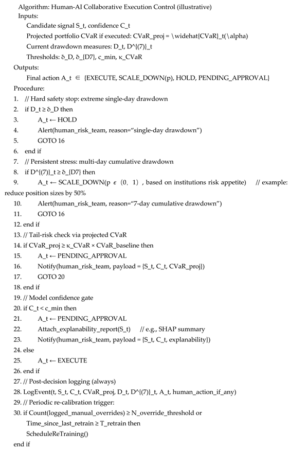
The algorithm implements layered risk controls: (i) immediate hard stops on extreme single-day drawdown to prevent catastrophic loss propagation; (ii) multi-day persistent stress controls () to limit exposure under trending adverse regimes; (iii) a projected CVaR gate that assesses the tail-loss implication of executing a candidate signal given current portfolio composition and market conditions; and (iv) a model-confidence gate that routes low-confidence signals to human review. Layering reduces the probability that a single failure mode (e.g., a miscalibrated confidence score) will produce an unchecked catastrophic action.
Using as a pre-execution filter aligns the deployment process with the paper’s emphasis on tail-risk control: signals implying an unacceptable increment in projected CVaR are subject to manual approval or suppression before execution. The multiplier can be set relative to an institution baseline CVaR or to absolute regulatory limits.
When a signal is escalated for manual approval (either due to low confidence or excessive projected CVaR), the system should attach a brief explanability digest (e.g., top SHAP feature contributions or a short permutation-importance summary). This supports human evaluators in assessing whether the signal has economically plausible drivers rather than spurious data artifacts.
Every execution decision and manual override is logged with context (signal, confidence, projected CVaR, drawdowns, human action). Logged events enable two governance functions: (i) ex-post auditability and compliance reporting; and (ii) creation of a curated set of human-labelled events that can be incorporated into periodic retraining to reduce repeated misclassification or model drift. The retraining trigger may be based on counts of manual overrides or on calendar intervals .
Thresholds , , and are institution- and strategy-dependent. Recommended starting values (illustrative only) are: =3% (single-day drawdown), (7-day cumulative), =0.6 (confidence), and =1.2 (no more than 20% increase over baseline CVaR). These should be stress-tested under alternative scenarios and refined via rolling-window backtesting.
Any human-intervention policy introduces latency and potential missed opportunities. The governance design should balance operational risk reduction against execution slippage and capacity constraints. For high-frequency contexts, the framework can be adapted to lighter-touch rules (e.g., automated scaling multipliers) while preserving audit logging and periodic human review.
This algorithm operationalizes the human-AI governance principles advocated above: it preserves the analytical advantages of ML signal generation while imposing explicit, auditable risk controls and human judgment checkpoints that address tail-risk, interpretability and regulatory transparency. Implementing such controls is consistent with the robustness checklist and CVaR-centric risk posture discussed in Section 3 and Section 5 of this manuscript.
Exhibits 2.
The Structure of the Human-AI model.
4.2.5. The Robustness of Human-AI Collaboration and Its Prospects
In summary, under the framework of collaborative statistical arbitrage dominated by artificial intelligence, assisted by human expertise, and continuous learning of human behavior in artificial intelligence models in human intervention, statistical arbitrage can take into account the efficiency of high-frequency strategies and the stability in extreme situations. Artificial intelligence provides efficient and systematic decision-making capabilities at the level of signal generation and execution; while human intelligence provides irreplaceable guarantees for risk identification, institutional compliance and explanatory verification. The cooperation between the two can not only effectively prevent algorithm overfitting and signal drift, but also maintain system stability through manual intervention in the black swan event, so as to achieve a balance between income, stability and compliance (Ning, 2024; Yuan, 2024; OECD & FSB, 2024).

Table 1.
Comparison of Traditional, ML-Based and Human-AI Collaborative Statistical Arbitrage Frameworks.
Table 1.
Comparison of Traditional, ML-Based and Human-AI Collaborative Statistical Arbitrage Frameworks.
| Dimension | Traditional Statistical Arbitrage | Machine Learning-Based Statistical Arbitrage | Human-AI Collaborative Framework (This study) |
| Core Decision Logic | Rule-based, econometric or parametric assumptions | Data-driven black-box or semi-black-box models | Hybrid: Algorithmic prediction + human strategic judgment |
| Interpretability | High (transparent mathematical structure) | Low to medium(model-dependent) | Medium to high (AI + human oversight + explanability tools) |
| Tail Risk Control | Weak or indirect | Medium (depends on optimization constraints) | Strong (explicit CVaR screening + drawdown monitoring + human intervention) |
| Robustness to Structural Breaks | Low | Medium (If retrained frequently) | Strong (explicit CVaR screening + drawdown monitoring + human intervention) |
| Response to Extreme Events | Poor | Unreliable/unstable | Adaptive and flexible (human-in-the-loop decision override) |
| Overfitting Risk | Low to medium | High (especially in deep models) | Controlled (human validation + stress scenario filtering) |
| Regulatory Transparency | Medium | Low | High (traceable logic + explainable risk process) |
| Ethical/Accountability Layer | Limited | Ambiguous | Clear (human accountability embedded in decision chain) |
| Practical Implementability | High | Medium to high | High (combines automation with portfolio manager control) |
| Long-term Stability | Medium | Uncertain | High (multi-layer risk governance loop) |
Note: This comparison highlights that while traditional and purely machine learning–based statistical arbitrage strategies each possess distinct advantages, they also suffer from critical limitations under conditions of heightened uncertainty and tail-risk exposure. The proposed Human–AI collaborative framework integrates computational efficiency with human risk awareness, thereby enhancing interpretability, robustness, and regulatory friendliness. This hybrid architecture is particularly suited for modern financial environments characterized by regime shifts, extreme volatility, and heightened demand for transparent decision-making.
5. Conclusion
The practice of statistical arbitrage has undergone a profound transformation, shifting from predominantly linear, econometric formulations toward increasingly data-driven and algorithmic paradigms. Machine learning and reinforcement learning significantly expand the analytical toolkit available to quantitative traders, enabling the detection of complex, nonlinear dependencies and the construction of highly scalable strategies. Yet this evolution also intensifies critical challenges, including model overfitting, opacity in decision-making processes and vulnerability to extreme market conditions. Simultaneously, fundamental constraints such as transaction costs, liquidity limitations and regulatory requirements continue to exert a decisive influence on realised performance.
5.1. Summary
In this context, we advocate a pragmatic human-AI collaborative approach, in which advanced models are complemented by human judgement capable of enforcing risk thresholds, interpreting regime shifts and enhancing accountability. Such integration not only improves robustness but also addresses growing demands for transparency and governance in algorithmic decision-making.
More broadly, this paper argues that the future of quantitative trading and risk management does not lie in the pursuit of fully autonomous systems, but rather in the intelligent integration of algorithmic efficiency and human strategic oversight. By embedding CVaR-based screening and discretionary intervention into the decision-making process, the Human–AI collaborative framework moves beyond optimization toward responsibility, transparency, and resilience. In this sense, it provides a conceptual blueprint for next-generation risk governance in data-intensive financial markets. Further empirical development of this architecture across asset classes and market conditions represents a promising direction for future research.
Looking forward, three research directions appear especially promising: the development of adaptive, risk-aware learning algorithms capable of controlling tail exposure; the incorporation of richer, multimodal data sources to enhance contextual awareness; and continued progress in explainable artificial intelligence to support regulatory alignment and institutional trust. Advancing along these paths will contribute not only to more effective trading strategies, but also to a safer, more transparent and more sustainable application of automation within modern financial markets. This perspective is particularly aligned with the growing emphasis on risk governance and model accountability in contemporary financial regulation.
5.2. Limitations
This study offers a conceptual synthesis and operational framework but does not present exhaustive institution-level backtests. The framework’s thresholds and governance mechanisms require calibration to specific trading universes and institutional constraints. Future empirical work should perform large-scale, out-of-sample validation and make code/data publicly accessible to strengthen reproducibility.
Acknowledgments
I hereby express my sincere gratitude to all authors of the literature cited in this thesis, whose rigorous research findings and profound academic insights have laid a solid theoretical foundation for the completion of this study.
References
- Alexander, C., Chen, X., Deng, J., & Wang, T. (2024). Arbitrage opportunities and efficiency tests in crypto derivatives. Journal of Financial Markets, 71, 100930. [CrossRef]
- Avellaneda, M., & Lee, J.-H. (2010). Statistical arbitrage in the US equities market. Quantitative Finance, 10(7), 761–782. [CrossRef]
- Balladares, K., Ramos-Requena, J. P., Trinidad-Segovia, J. E., & Sánchez-Granero, M. A. (2021). Statistical Arbitrage in Emerging Markets: A Global Test of Efficiency. Mathematics, 9(2), 179. [CrossRef]
- Bollerslev, T. (1986). Generalized autoregressive conditional heteroskedasticity. Journal of Econometrics, 31(3), 307–327. [CrossRef]
- Caneo, F., & Kristjanpoller, W. (2021). Improving statistical arbitrage investment strategy: Evidence from Latin American stock markets. International Journal of Finance & Economics, 26(3), 4424–4440. [CrossRef]
- Ciacci, A., Sueshige, T., Takayasu, H., Christensen, K., & Takayasu, M. (2020). The microscopic relationships between triangular arbitrage and cross-currency correlations in a simple agent based model of foreign exchange markets. PLOS ONE, 15(6), e0234709. [CrossRef]
- Coache, A., Jaimungal, S., & Cartea, Á. (2023). Conditionally Elicitable Dynamic Risk Measures for Deep Reinforcement Learning. SIAM Journal on Financial Mathematics, 14(4), 1249–1289. [CrossRef]
- De Moura, C. E., Pizzinga, A., & Zubelli, J. (2016). A pairs trading strategy based on linear state space models and the Kalman filter. Quantitative Finance, 16(10), 1559–1573. [CrossRef]
- Dickey, D. A., & Fuller, W. A. (1979). Distribution of the Estimators for Autoregressive Time Series with a Unit Root. Journal of the American Statistical Association, 74(366a), 427–431.
- Do, B., & Faff, R. (2010). Does Simple Pairs Trading Still Work? Financial Analysts Journal, 66(4), 83–95. [CrossRef]
- Elliott, R. J., Van Der Hoek , J., & Malcolm, W. P. (2005). Pairs trading. Quantitative Finance, 5(3), 271–276.
- Engle, R. (2002). Dynamic Conditional Correlation: A Simple Class of Multivariate Generalized Autoregressive Conditional Heteroskedasticity Models. Journal of Business & Economic Statistics, 20(3), 339–350.
- Engle, R. F., & Granger, C. W. J. (1987). Co-Integration and Error Correction: Representation, Estimation, and Testing. Econometrica, 55(2), 251. https://doi.org/10.2307/1913236. [CrossRef]
- Frino, A., Mollica, V., Webb, R. I., & Zhang, S. (2017). The impact of latency sensitive trading on high frequency arbitrage opportunities. Pacific-Basin Finance Journal, 45, 91–102. [CrossRef]
- Gatev, E., Goetzmann, W. N., & Rouwenhorst, K. G. (2006). Pairs Trading: Performance of a Relative-Value Arbitrage Rule. Review of Financial Studies, 19(3), 797–827. [CrossRef]
- Greenwald, B. C., & Stein, J. C. (1991). Transactional Risk, Market Crashes, and the Role of Circuit Breakers. The Journal of Business, 64(4), 443. [CrossRef]
- Han, C., He, Z., & Toh, A. J. W. (2023). Pairs trading via unsupervised learning. European Journal of Operational Research, 307(2), 929–947. [CrossRef]
- Hochreiter, S., & Schmidhuber, J. (1997). Long Short-Term Memory. Neural Computation, 9(8), 1735–1780.
- Hogan, S., Jarrow, R., Teo, M., & Warachka, M. (2004). Testing market efficiency using statistical arbitrage with applications to momentum and value strategies. Journal of Financial Economics, 73(3), 525–565. [CrossRef]
- Hong, H., & Stein, J. C. (2007). Disagreement and the Stock Market. Journal of Economic Perspectives, 21(2), 109–128.
- Jaimungal, S., Pesenti, S. M., Wang, Y. S., & Tatsat, H. (2022). Robust Risk-Aware Reinforcement Learning. SIAM Journal on Financial Mathematics, 13(1), 213–226. [CrossRef]
- Jarrow, R., Teo, M., Tse, Y. K., & Warachka, M. (2012). An improved test for statistical arbitrage. Journal of Financial Markets, 15(1), 47–80. [CrossRef]
- Jegadeesh, N., & Titman, S. (1993). Returns to Buying Winners and Selling Losers: Implications for Stock Market Efficiency. The Journal of Finance, 48(1), 65–91.
- Johansen, S. (1988). Statistical analysis of cointegration vectors. Journal of Economic Dynamics and Control, 12(2–3), 231–254. [CrossRef]
- Krauss, C., Do, X. A., & Huck, N. (2017). Deep neural networks, gradient-boosted trees, random forests: Statistical arbitrage on the S&P 500. European Journal of Operational Research, 259(2), 689–702. [CrossRef]
- Lin, B., & Tan, Z. (2023). Exploring arbitrage opportunities between China’s carbon markets based on statistical arbitrage pairs trading strategy. Environmental Impact Assessment Review, 99, 107041. [CrossRef]
- Lütkebohmert, E., & Sester, J. (2021). Robust statistical arbitrage strategies. Quantitative Finance, 21(3), 379–402. [CrossRef]
- Marshall, B. R., Nguyen, N. H., & Visaltanachoti, N. (2013). ETF arbitrage: Intraday evidence. Journal of Banking & Finance, 37(9), 3486–3498. [CrossRef]
- Murphy, N., & Gebbie, T. (2021). Learning the dynamics of technical trading strategies. Quantitative Finance, 21(8), 1325–1349. [CrossRef]
- Nasekin, S., & Härdle, W. K. (2019). Model-driven statistical arbitrage on LETF option markets. Quantitative Finance, 19(11), 1817–1837. [CrossRef]
- Piotrowski, E. W., & Sladkowski, J. (2004). Arbitrage risk induced by transaction costs. Physica A: Statistical Mechanics and Its Applications, 331(1–2), 233–239. [CrossRef]
- Ramos-Requena, J. P., Trinidad-Segovia, J. E., & Sánchez-Granero, M. Á. (2020). Some Notes on the Formation of a Pair in Pairs Trading. Mathematics, 8(3), 348. [CrossRef]
- Rousseeuw, P. J., & Croux, C. (1993). Alternatives to the Median Absolute Deviation. Journal of the American Statistical Association, 88(424), 1273–1283.
- Serrano, C., & Hoesli, M. (2012). Fractional Cointegration Analysis of Securitized Real Estate. The Journal of Real Estate Finance and Economics, 44(3), 319–338. [CrossRef]
- Stephenson, J., Vanstone, B., & Hahn, T. (2021). A Unifying Model for Statistical Arbitrage: Model Assumptions and Empirical Failure. Computational Economics, 58(4), 943–964. [CrossRef]
- Troyanskaya, O., Cantor, M., Sherlock, G., Brown, P., Hastie, T., Tibshirani, R., Botstein, D., & Altman, R. B. (2001). Missing value estimation methods for DNA microarrays. Bioinformatics, 17(6), 520–525. [CrossRef]
- Vergara, G., & Kristjanpoller, W. (2024). Deep reinforcement learning applied to statistical arbitrage investment strategy on cryptomarket. Applied Soft Computing, 153, 111255. [CrossRef]
- Zhang, W., Li, S., Guo, Z., & Yang, Y. (2023). A hybrid forecasting model based on deep learning feature extraction and statistical arbitrage methods for stock trading strategies. Journal of Forecasting, 42(7), 1729–1749. [CrossRef]
- Kanamura, T. (2025). Sustainability arbitrage pricing of ESG derivatives. International Review of Financial Analysis, 104, 104177. [CrossRef]
- Bailey, D. H., & Lopez De Prado, M. (2014). The Deflated Sharpe Ratio: Correcting for Selection Bias, Backtest Overfitting and Non-Normality. SSRN Electronic Journal.
- Fischer, T., & Krauss, C. (2018). Deep learning with long short-term memory networks for financial market predictions. European Journal of Operational Research, 270(2), 654–669. [CrossRef]
- Flori, A., & Regoli, D. (2021). Revealing Pairs-trading opportunities with long short-term memory networks. European Journal of Operational Research, 295(2), 772–791. [CrossRef]
- Huck, N. (2019). Large data sets and machine learning: Applications to statistical arbitrage. European Journal of Operational Research, 278(1), 330–342. [CrossRef]
- Krauss, C., Do, X. A., & Huck, N. (2017). Deep neural networks, gradient-boosted trees, random forests: Statistical arbitrage on the S&P 500. European Journal of Operational Research, 259(2), 689–702. [CrossRef]
- Chow, Y., Ghavamzadeh, M., Janson, L., & Pavone, M. (2018). Risk-Constrained Reinforcement Learning with Percentile Risk Criteria. Journal of Machine Learning Research, 18, 1–51.
- Rockafellar, R. T., & Uryasev, S. (2000). Optimization of Conditional Value-at-Risk. Journal of Risk, 2(3), 21–42. [CrossRef]
- Ning, B. (2024). Advanced Statistical Arbitrage with Reinforcement Learning. arXiv preprint arXiv:2403.12180. [CrossRef]
- Rockafellar, R. T., & Uryasev, S. (2002). Conditional Value-at-Risk for General Loss Distributions. Journal of Banking & Finance, 26(7), 1443–1471. [CrossRef]
- Yuan, H. (2024). Alpha-GPT 2.0: Human-in-the-Loop AI for Quantitative Investment. arXiv preprint arXiv:2402.09746.
- Mosqueira-Rey, E., Hernández-Pereira, E., Alonso-Ríos, D., Bobes-Bascarán, J., & Fernández-Leal, Á. (2023). Human-in-the-loop Machine Learning: A State of the Art. Artificial Intelligence Review, 56, 3005–3054. [CrossRef]
- OECD & Financial Stability Board (FSB). (2024). OECD–FSB Roundtable on Artificial Intelligence (AI) in Finance: Summary of Key Findings.
Disclaimer/Publisher’s Note: The statements, opinions and data contained in all publications are solely those of the individual author(s) and contributor(s) and not of MDPI and/or the editor(s). MDPI and/or the editor(s) disclaim responsibility for any injury to people or property resulting from any ideas, methods, instructions or products referred to in the content. |
© 2025 by the authors. Licensee MDPI, Basel, Switzerland. This article is an open access article distributed under the terms and conditions of the Creative Commons Attribution (CC BY) license (http://creativecommons.org/licenses/by/4.0/).
Copyright: This open access article is published under a Creative Commons CC BY 4.0 license, which permit the free download, distribution, and reuse, provided that the author and preprint are cited in any reuse.


