Impact of Economic Drivers and Climate Change Policies on the Stability of French Pension System

Nicolas Houlie

doi:10.20944/preprints202512.1286.v1

Submitted:

12 December 2025

Posted:

15 December 2025

You are already at the latest version

Abstract

In this paper, I present a machine learning (ML) model, trained using the dataset pre-sented by the “Conseil d’Orientation des Retraites” (COR), that simulates pension ex-penditures for France for the period 2025-2070 for 12 scenarios. Six of these scenarios are presented for the first time in this study, and another six were proposed by the Network for Greening the Financial System (NGFS) initiative. The main result of this study in-dicates that Life Expectancy at 65 (LE@65) is not the most significant variable for planning pension expenditures over the next decades. LE@65 is only the most important ex-penditure driver under some conditions (e.g. productivity < 0.7%). For higher values of productivity, LE@65 is only a second-order variable, which is superseded by others, such as GDP and then social costs. Additionally, I show that GDP growth is crucial to the system stability, while the type of production and inflation trends also play a significant role. At last, predictions based on the NGFS scenarios suggest that climate change policies will have a substantial impact on the French pension system through a series of shocks on GDP until 2050.

Keywords:

French pension system

;

Conseil Orientation des Retraites

;

pensions

;

climate change

;

NGFS

Subject:

Business, Economics and Management - Economics

Introduction

The reform of the pension system is one of the favorite topics of the national political elite in France for four decades (Blanchet, 2010; Boulhol, 2019; Boulhol and Queisser, 2023; Sterdyniak et al., 1999). Indeed, for all political groups, it does symbolize what should be preserved at all costs or reformed drastically. In comparison to other system, the French pension system is specific as 1/ it was a long awaited system (Aleksandrova, 2020; Blanchet, 2020; Dumons, 1994; Dumons and Pollet, 1991; Thiveaud, 1997), 2/ it was established in the aftermath of World WW2 by political forces which survived the nazi occupation and 3/ the capitalization is quasi-absent, the solidarity between generations is pushed to its maximum: current workers’ pay for the retirement costs of currently retired population with very few amount invested in long-term equity investment (Bayar, 2013; Chardon-Boucaud and Ramuzat, 2022). I note that since the reform made in the nineties, the financing of the system is provided by multiple sources of funding such as consumption taxes, wealth taxes, and social contribution computed from individual wages. If the recourse to alternative sources of financing (e.g. foreign tourists, levied taxes with clear attribution, etc.) make sense when it is intended to lower the tax burden of the private sector, it is however making the financing negotiations rounds harder to complete and harder to pilot (e.g. an account link between consumption and tourism is made with French pensions expenditures)¹.

It is well accepted that it is challenging to model the cost of pensions over various time horizons because for instance of the changes in the system (reforms, lower taxes) initiated since the 1990s, a large number of soon-to-be retirees’ response to reforms, and careers of workers are more disrupted than before. Nevertheless, various French institutional bodies started to model expenses using microsimulation tools in 1990s (Bellanger and Goujon, 2020; Blanchet, 2011; Blanchet et al., 2011; Duc et al., 2015; Duc et al., 2013) including the “Direction Générale du Trésor” through the ageing report of 2018-2024 exercises that are submitted to the European Commission every three years. The outcome of these initiatives confirmed that the challenge to estimate the long-term expenses was indeed immense (Figure 1 for a comparison of models published by two institutions over the same time span). For the models shown in Figure 1, the differences between models is approximately 0.25% of GDP (€ 6.5 billion per year in 2023; I will use these values later in the article to produce more robust training datasets).

In parallel to the modelling effort by the government services, and in an attempt to canalize the political debate after the 1993 reform which led to a delay in the effective retirement age (Bozio, 2006, 2008; Duc, 2015), the French government has created the “Conseil d’Orientation des Retraites” (COR). The COR is an institution that gathers experts, union representatives, and parliamentary members, to advise the government on the stability of the pension system. I note the data provided to the COR to model the pension expenditures largely come from institutions that depend directly on the government (e.g., INSEE). Although the data used in the models are independently and professionally collected, the economic scenarios used are proposed by the government itself. For instance, only one GDP trend is given for the simulations, and only some evolutions of productivity (n=4) are considered. Also, the trends of variables are linearly developing (i.e., models with increasing and then decreasing productivity are not available today). At last, scenarios with increasing social contributions (from companies and households) and scenarios including climate change impact are not available. One can imagine this limitation of the dataset is due to the available resources allocated to this exercise, to the differing political views on the future but ultimately the completeness of the scenarios envisaged is therefore reduced.

Following the approach proposed by (Houlié, 2025) for predicting House Prices using macro-economic indicators, I use ML to simulate both the government’s and the economic system’s behavior impact on the stability of the pension system. The Machine Learning (ML) model obtained, based on data published by the COR, enables the use of alternative data (GDP values, productivity series, etc.). I used the trained model to simulate 1/ six macro-economic scenarios that are not included in the existing COR scenario dataset and 2/ six scenarios which are based on the GDP output published by the NGFS in 2025. The output of those models suggests it is possible to predict expenditures by disturbing the COR original datasets in order to simulate other scenarios, and that Climate Change cannot be ignored when considering the stability of the system.

Data

Original dataset

For the training of the models, I have used the dataset published by the COR on its website in June 2025. This dataset is dated of 2024. The COR was established in 2000, and chose the oldest data point available is of 2002. Periods of significant economic growth (1950-2001) are therefore not available to train the model. As stated before, each COR scenario follows a trajectory that relies on the assumptions made by the political sphere. Hence, some trajectories are arbitrarily designed (e.g., public expenses progression, contribution of the state, GDP curves, productivity curves), although they contain a segment of observed data (black circles in Figure 2).

All scenarios assume no increase in legal immigration (and the social contribution associated with it), no birthrate increase, and no pandemic can happen in the period 2040-2070, which implies the population will tend to decrease by 2070 (from 2025 to 2070: average of -0.1% per year, a total decrease of 1.1% by 2070). This is in contradiction with the estimates for France made by World Population Prospects report published in 2024 (~68 millions²) or with Eurostat estimates (69.66 millions 2070³) for the year 2070. One expects such uncertainty in the country’s population to affect total workers, GDP estimates, and taxes levied, regardless of the ratio between active and retired populations. As consumption taxes are used to finance the pension system, we expect the population, migrants and tourists amount consuming in France to contribute to their part to the system.

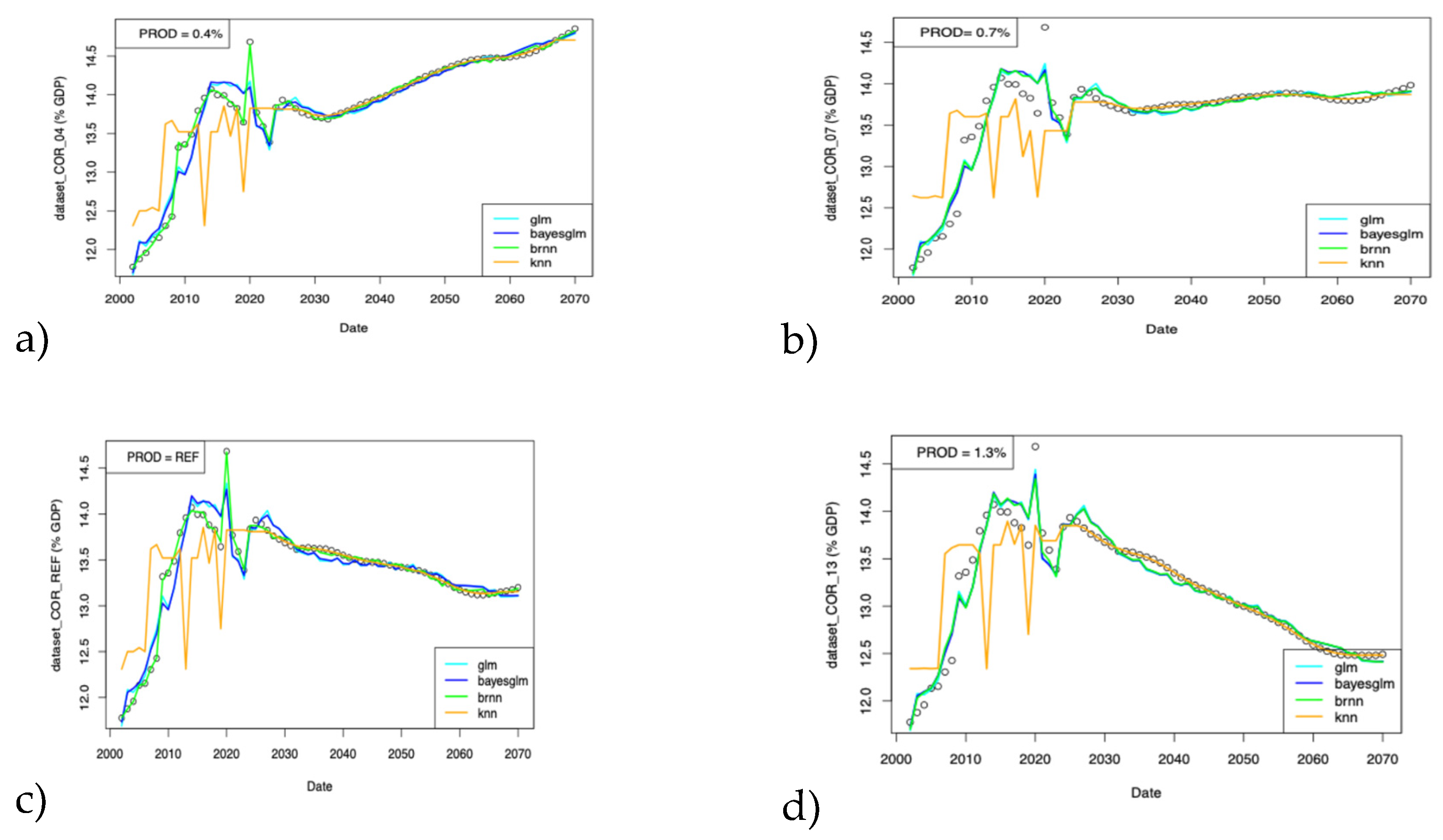
The four main COR scenarios are assuming productivity of 0.4%, 0.7%, 1.0 and 1.3%. Until recently the productivity for France was known to be close to 1.3%. Therefore, one can assume that three of the four scenarios are pessimistic regarding this variable over a long-term horizon and difficult to predict on the short-term as observed during the COVID crisis (Askenazy et al., 2024; Coquet and Heyer, 2025).

Figure 3. Excerpt of data from the COR_REF scenario dataset. In this scenario, the social contributions are aimed to decrease until 2070, when a value of ~28.5% value is aimed. This evolution will happen while both measures of GDP will increase steadily, and state contribution will decrease to 1%. In this scenario, expenses are expected to decline steadily until 2070, reaching approximately 13% of GDP. Colors range from red (2002) to violet (2070).

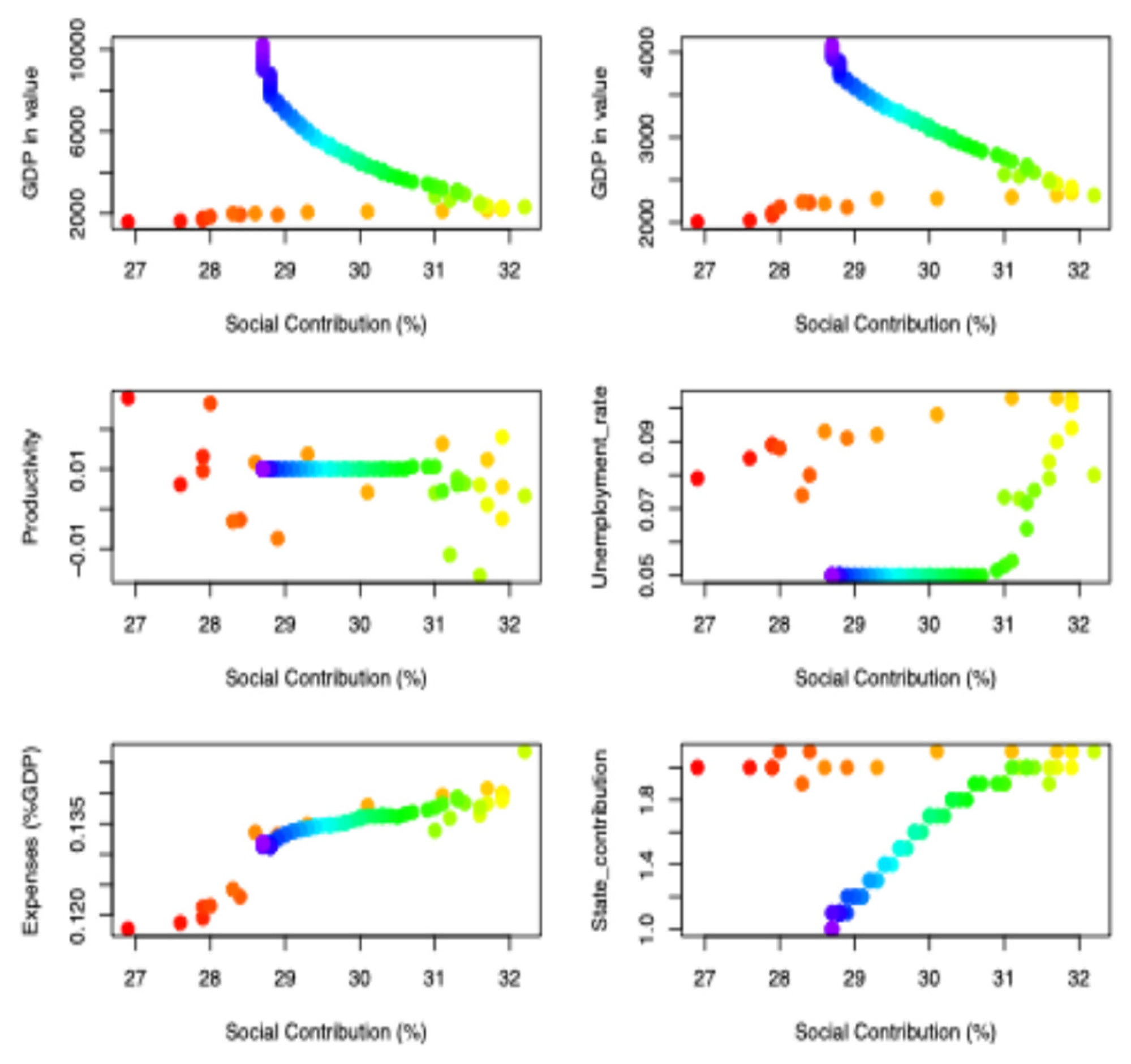
The reference scenario (“REF”, 1.0% productivity) presents some assumptions on the contribution of companies and employees and states which are interesting to point out. First, while the wealth produced increases steadily and productivity remains at 1% per year, social contributions decrease steadily. Second, the inflation is kept at about 2% per year, which is well aligned with the European Central Bank mandate. At last, the cause underlying the percentage of GDP ratio decrease is not explained by the government and might conflict with the view of French workers which see the pensions as a differed salary.

Dataset used for training

Each data of each variable was normalized⁴, and no other transformation has been applied. From the large dataset available with the COR dataset, I have selected ten variables to estimate the pension cost expressed as a percentage of GDP. Those variables encompass both demographic and economic contexts, which help to nourish the political and media debate. Variables chosen are the following: Productivity, Unemployment_rate, Migration_count, Fecondity, _Expectancy_at_65_women, Life_Expectancy_at_65_men, GDP (value), Social_contribution, State_contribution, GDP (volume).

Results

Observations

Before modelling the data, an exploration of the dataset allows for some observations to enrich the political debate. First, the pensions expenditures are not always correlated life expectancy at 65 (LE@65) as stated repeatedly in the public debate (Figure 4 and Table 1). In fact, only one COR scenario (productivity = 0.4% per year) shows an increase of expenditures increase with the life expectancy at 65 (for both men and women). This first observation suggest that when economic productivity increases, social contributions and salaries progress faster than the expenditures necessary to stabilize pension system. Nowadays, productivity gains are close to 1% and were, until recently, assumed as 1.3% in European pension simulations (Eurostats). The recent decrease in productivity, which followed the COVID pandemic in France, is expected to resolve itself compared to other European countries (see INSEE report). A vivid job market also likely tends to increase the wages which in turn increases the social contribution amount.

Correlation coefficients between life expectancies and pension costs for each productivity level across the scenarios are shown in Table 1. Those scenarios confirm that the economic activity allows for the stability of the system and less the distribution of ages across the population: a largely young and non-productive population would not allow for the sustainability of the system.

Regression model

For the sake of comparison with models later presented in the study and for users less prone to sophisticated methods, I have made two linear models which are showing the dependence of the pension expenditures to each variable. The first version of the model takes the data-as-is (Table 2) as the second version is using log-normal version of the data (Table 3).

The explanatory power of both models is good (RMS<0.01; Figure 5), and residuals are well below the differences between models shown in (Figure 1). Some features can be observed and should be compared with more sophisticated model outputs. Both models indicated a different dependance to LE@65 for men and women: LE@65 for men is increasing with costs while the increase of LE@65 for women tends to decrease the expenditures. As the pension costs depend on both of the situation of men and women during their career and their marital status at the time of the death of the first spouse, I could expect that women tend to benefit less from the retirement system as their husband tend to survive longer times (the difference between LE@65 decrease from 4.5 to 3.7 years between 1994 and 2024 according to INSEE). For example, in some configurations, the minimum wage pension may be smaller than the reversion pension received after the death of their husband and may create this effect. There is therefore a need to pilot the LE@65 for men and women independently.

Models also suggest that GDP in volumes is a strong contributor to the system evolution, and that GDP in values (including the price effect) has an opposite impact. This suggests that the number of workers involved in the social contribution (~60% of the total of pension spent) is important, somewhat more important than the increase in the value of the economy transferred during a year (GDP in value). Conversely, this observation could be supported by the recent trend of deindustrialization of the country over the same period which may tend to produce less volume of goods but with more value and less workers.

First ML models

Training based on single scenarios

I have first trained the models using each COR scenario dataset independently. For each four scenario (distinguished on productivity series), I have tested 4 methods to train the model: generalized linear model “glm”, bayesian generalized linear model “bayesglm”, bidirectional recurrent neural network “brnn”, and k-nearest neighbor “knn”. The visual inspection of the results (Figure 2) suggests that from the four strategies, only “knn” is underperforms in fitting individual COR scenarios. After excluding the “knn” methodology, I conclude that model can reach the same performance whatever the 3 methodologies used.

Figure 6. Performance of various methods for the four main scenarios (a-d) presented in the June 2025 COR report.

The analysis of the most important variables is shown in Table 4, for the Bayesian GLM methodology. From the four datasets used as a training set, one dataset led to a model favoring the LE@65 within the two first most important parameters. The other models favour either social contributions or GDP in value. LE@65s are still important, but fall rather in second place by some percentage points.

Training on complete dataset

To detect potential overfitting of the models because of the lack of data, I then joined the four main COR datasets to train a model on a larger dataset. This operation allows for increasing the size of the dataset, and if successful will allow to predict expenditures for context corresponding to in-between scenarios (e.g. productivity at 0.9%, scenario expenses for time-varying GDP growth).

A set of new trainings is then completed for the same methodologies (Figure 7) and for a training dataset prepared with 75/25 ratios.For each methodology, 1000 re-trainings were made with the 75% complete dataset (data of the four main scenarios) and compared with the prediction obtained using the test dataset (25% of complete dataset). As for the previous model the “knn” methodology shows the worst performance as it is not able to model well the scenario with productivity at 1.3%. The other 3 methodologies are able to “jump” from one scenario to another after being trained with the dataset made of the combination of the four main scenarios. Theses results suggest it is possible to use those models to predict new scenarios: for instance we could take the COR scenario corresponding to the 1.3% productivity for 10 years and then switch to the reference scenario for the rest of the time windows. Model capabilities shown in Figure 7 suggest expenditures of discontinuous scenarios could be well estimated.

As for previous models, I have completed a variable importance analysis. I remind here that the polarity (sign of the contribution) of each variable is not addressed here. For instance, the contribution of higher GDP in volume is anticorrelated with expenses while, Life expectancy at 65 for men is correlated with expenses. None of the four methodologies suggests LE@65s are the most important parameters. This result highlights a weakness of the usual political debate about the pension system, which assumes that the GDP is of secondary importance, and only LE@65s are driving the stability of the system. Tehe GDP_vol is always within the three most important parameters whatever methodology is used.

The fact that GDP_vol has a stronger relative importance than GDP_val suggests that producing more goods is more important than producing more expensive goods (e.g. luxury, aerospace), and maybe the number of workers involved also plays a role in the system's stability.

Table 5. Average variable importance (%) after 1’000 data train-test dataset splits for each of the four methods (“brnn”, “GLM”, “knn” and “Bayesian GLM”) and 10 variables considered in this study. The three most important variables for each methodology are indicated by bold fonts. GDP_vol, GDP_val, LE@65 women, and LE@65 men represent more than >75% relative importance except for the GLM methodology (approx. 45%).

	BRNN		GLM		“knn”		Bayesian GLM
Variable	Value (%)	Unc. (%)	Value (%)	Unc. (%)	Value (%)	Unc. (%)	Value (%)	Unc. (%)
GDP VOL	100.0	0.2	72.0	3.5	100.0	0.2	100.0	0.3
LE@65 men	97.1	1.6	31.4	2.7	97.1	1.5	97.1	1.5
LE@65 women	84.6	1.4	30.0	2.7	84.6	1.3	84.6	1.3
Social contribution	81.7	2.9	100.0	0.0	81.3	2.8	81.6	2.9
GDP val	71.7	1.8	17.9	2.4	71.6	1.8	71.7	1.8
Productivity	15.3	2.6	1.1	1.7	15.3	2.6	15.2	2.6
Birth rate	5.1	1.0	2.2	1.5	5.1	1.0	5.2	1.0
Unemployment	1.2	0.7	29.4	2.3	1.3	0.7	1.2	0.7
Migration count	0.2	0.3	44.4	2.4	0.2	0.4	0.2	0.3
State contribution	0.1	0.3	1.5	1.8	0.1	0.2	0.1	0.2

New time-series of expenses based on the Bayesian-GLM-trained model

From this point in the study, I chose to use the Bayesian GLM model, which is amongst the best performing methods of the set tested so far, and because it is well adapted to the dataset used. Now the BGLM model is trained, it is possible to quantify the sensitivities of the model to shocks. I have chosen four variables (LE@65s, GDP in volume and GDP in value) to be shocked arbitrarily (Figure 8). Interestingly, such sensitivity analysis confirms the first linear model shown above: changes in LE@65 for men and women have opposite effects, as do GDP_vol and _val. A decrease in expenses may therefore come from a decrease in LE@65 for men, or a decrease in the GDP in value. I conclude from these sensitivity tests that all models so far are showing the same outcome with similar variable contributions.

Models based on 4 variables and using older data (1990-2001)

Models depends on the data used but when the size of dataset is decreased while model performance is preserved, it measms some of the data used so far was not necessary. As shown before, for the Bayesian GLM, 77% of the relative variable importance can be attributed to the GDPs and life expectancies variables. I test here it is possible to use less variables to explain the data as well as before. I then trained two others models which are using only four variables (GDP in volume and in value, and Life expectancies at 65 for both sexes). This operation allows for the time extent of the dataset to older years, beyond the scope covered by the COR.

In order to prepapre the data, some operation were necessary to be completed. As in the 90s the life expectancy was increasing linearly for both men and women, it was easy to extrapolate those time-series for those two variables. For GDP, it was more challenging as only GDP in value was available from the FRED database. However, one must admit that GDP variables are highly linear with time. GDP in volume had to be reconstructed by polynomial fit (degree 3) and extrapolation for the period [1990-2001]. The model had to be trained again (red curve to be compared to observed data in Figure 9).

It is clear that those models may be less data-rich than the ones previously presented. However, the performance of the models is acceptable with a 0.3% GDP of scattering around the reference model expenditures (Figure 9). They allow 1/to extend the time span covered and 2/to expand this approach to other countries such as Switzerland (AVS model) without losing too much explanatory power.

Predictions based on six politico-economic scenarios

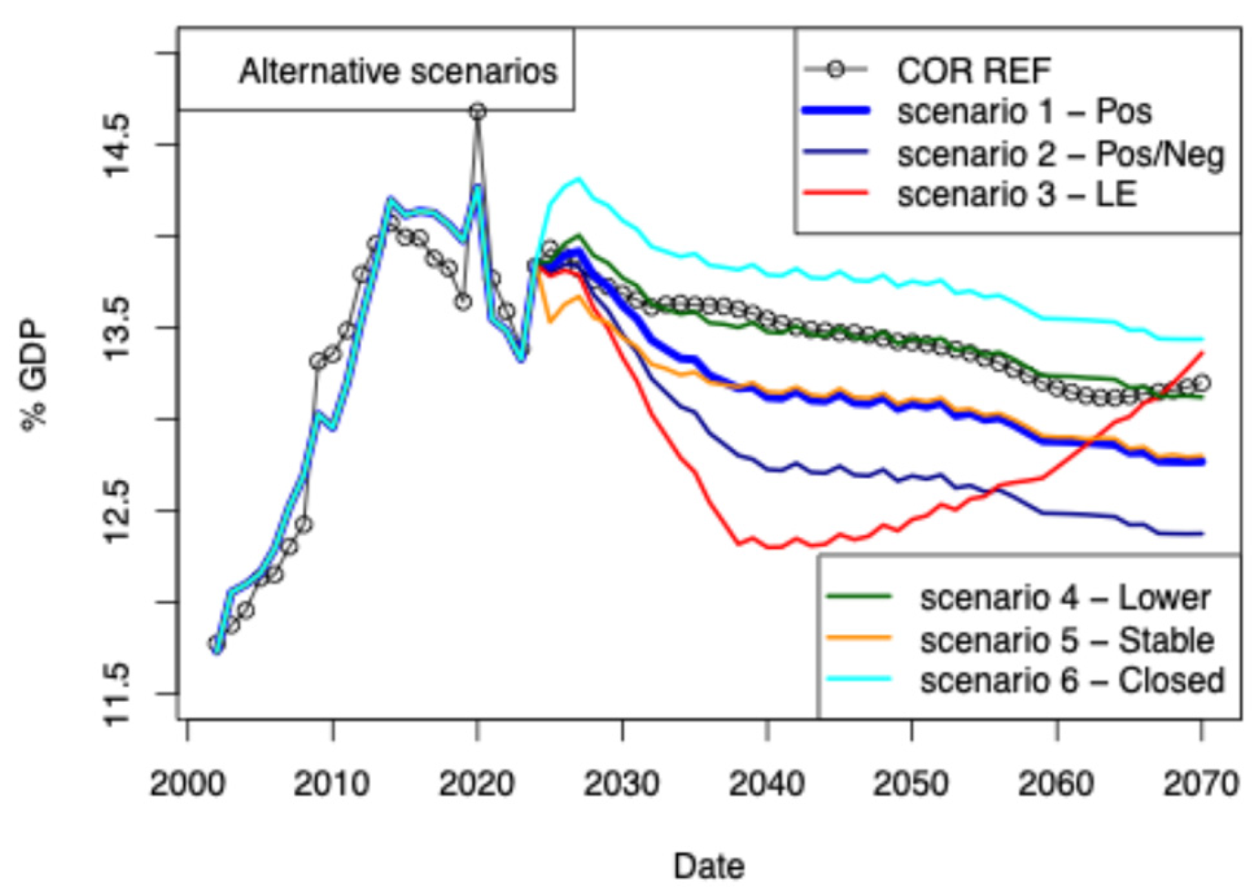
I present 6 scenarios which are designed to cover the topics mentioned in the media: migration, life expectancy, and economic performance (Table 6). The first two scenarios focus on varying the GDP curves and shock them with respect to the reference scenario. Those explore the impact of the GDP on the pension expenses. The third scenario focuses on keeping the Life Expectancy constant at the value of 2023. The last three scenarios aim to describe the impact of migration at three levels: a lower level (“Lower”, 100’000 people per year), the same level as today (“Stable”, 150’000 people per year), and a final level that forces migration to be close to 20’000 people per year (“Closed”). The 6th scenario also includes an impact on the GDP as we expect a high negative migration to have an impact on the GDP (lower national consumption, larger amount of imports).

Figure 10. Impact of the six scenarios presented in this section. Descriptions of the model are detailed in the main text. All models suggest the expenses will decrease from 2030. Spreads between models are multiples of 0.5% GDP per year (approx. 15bn euros per year in 2025). This value suggests the uncertainty of the predictions is close to this value.

Scenario 1 “Negative GDP shock then recovery”

Here we simulate a slow decrease of 5 % GDP in volume over 15 years which is then stopped and the progression is then similar to the reference scenario. This increase of GDP is associated with an inflation of 5% on top of the central scenario value, which is then stopped, and the progression is then similar to the reference scenario.

Scenario 2 “Positive GDP shock plus deflation”

This scenario is a “shock scenario” corresponding to an increase of GDP (+ 10% distributed over 15 years) and a decrease of prices (- 10% distributed over 15 years) over 3 election cycles and then a return to the reference GDP curves proposed by the French government.

Scenario 3 “Life expectancy stagnates”

In this scenario, both Life expectancies at 65 (LE@65) for men and women are maintained at their 2025 value until 2040 and then resume their progression afterwards. All other variables are kept unchanged implying that country wealth keeps progressing as in the central COR scenario. Context of this scenario: appearance of a new disease, loss of access to medication (shortage, or price barrier), or slower technical progress.

Scenario 4 “Migration is lower”

In this scenario, the migration level is decreased to 100’000 people per year for > 2025. All the other variables are kept at values of the central scenario. No shock on GDP is introduced.

Scenario 5 “Growth led by migration”

The migration level is maintained to 150’000 people per year until 2070, inducing a GDP_volume shock of 5% from 2025, and then a eolution of GDP corresponding to the original reference scenario. The GDP shock is unique and is not continued in time. One could argue this is not completely realistic but as the right level of GDP change is not known, I chose to keep this GDP shock as discrete.

Scenario 6 “Closing the borders”

This scenario corresponds a significant political shift, which, triggers a population migration away from the country, resulting in both a shock to GDP (decrease of consumption, leading to a deflation of prices ) and a decline in the population number (“solde migratoire negative”). The lower migration is inducing a strong decrease of prices over a year (-5%) and then a progression corresponding to the original reference scenario.

Those six economico-political scenario do not claim to be realistic, they just show the various possibles by linking political decisions to macro-economic indicators and their impact on the pension expenditures. As most of the political decision could have an impact on the GDP progression, those policies could be balanced by others (tax levies, confidence of households) which may also favour the increase of GDP. At last, those scenarios could be combined and lead to other conclusions at different horizons. One of the aspect which was not considered in those scenarios is climate change and this could be addressed at the NGFS (Network for Greening the Financial System) expressed their scenrios in percentage of GDP change. If we consider the French economy is following a global trend and its GDP would be as impacted as the global economy (french economy is well integrated) and considering the uncertainties on the GDP change estimates, it is possible to model climate change related scenarios using the model trained above using the BGLM methodologies.

Impact of Climate Change?

Over the next decades, we expect climate change to have an impact on the economies through shocks on the productivity, GDP and inflation. Due to climate change, we anticipate that crops will be disrupted, migrations will intensify, and economically productive areas will become deserted or increasingly difficult to maintain. All those local/regional effects may have a diffuse impact on the production, economic activity, prices, and public spending. Network for Greening the Financial System (NGFS) designed scenarios constraining the overall GDP impact for six paths of climate change adaption (Table 7). As the model trained using the COR data are sensitive to GDP trends, I have modelled the effect of the NGFS scenarios using the same model. The impact of models ranges from approx. 0.75% (Net Zero 2050) to 1.5% (current policies) of GDP per year (Figure 9). For the sake of simplicity, I have chosen to decrease the GDP in volume while we increased the GDP in value by the same percentage. Doing this corresponds to a loss of economic output while an increase in prices is observed over the same period. This scenario would be realistic for agricultural goods traded in international markets, which suffer from productivity losses attributed to climate change.

Figure 11. Impacts based on NGFS scenarios on the impact of Climate Change on GDP until 2050. Impact of the previous versions published by the same institution are also shown using grey color.

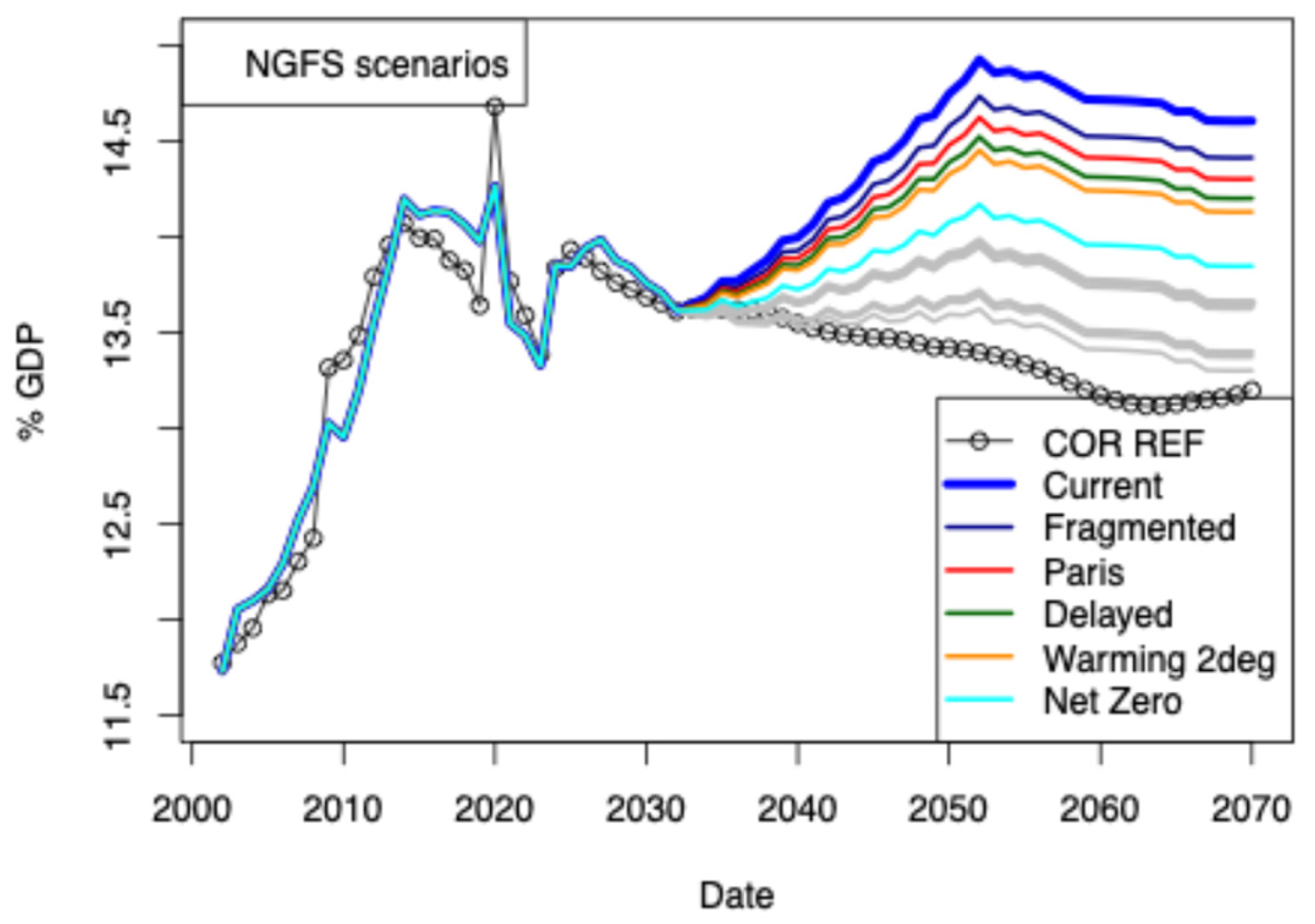
Adapting to climate change by keeping the same Current Policies has a similar effect to closing the border and shocking the GDP over a short time window: the GDP may never recover to its initial trend, leading to an impact of >0.1% GDP per year on the pension system. At the other extreme, the “Net Zero scenario” would have an effect on pension expenses that could be less than the difference between the pension system predictions made by the COR and the European Commission every year (approximately 0.25% of GDP). The other scenarios proposed by NGFS lie between those two extremes. The impact of those scenarios could be at least partially be combined with the first 6 scenarios presented in this study. However, the combination of extreme scenarios (scenario 6 + scenario A) should be carried out with caution as the training dataset do not contain such a large shocks, yet.

Discussion

Because received pensions are partially based on personal contributions computed from received wages, the system carries some inequalities (Aubert and Bachelet, 2012; Barnay, 2005; Bommier et al., 2003; Bonnet and Rapoport, 2020; Brocas, 2004; Buffeteau and Godefroy, 2005; Sterdyniak, 2005) which can only be addressed through solidarity of the working population. Solidarity is the only way to offer some protection from events potentially affecting us all (e.g. Climate Change impact), or affecting some of us very badly (e.g. life accident, illness). I need to underline that if GDP is important, one should consider that inequality of income exists (see Figure 9.8 in Piketty (2014)) and not all tax levied on various financial income are not yet attributed to financing the pension system. On the other hand, adding financing source may not help smooth political debate. One can admit, the diversification of financing sources completed in the 1990’s made the system more difficult to pilot as not all contributors are also participating to the current economic situation.

Salaries should also be looked at as there are the base of the system. As the wages in France did not progress more than 20% (constant euro; INSEE accessed on 26 Nov. 2025) for public (since 2009) and private sectors (since 1996), the social contributions did not increase beyond this rate and the consumption moderation (Aubert et al., 2012; Blake and Garrouste, 2012; Mohamed Ali Ben et al., 2022; Tréguier, 2021) did not help to increase the resources mobilized by the active population. One can consider that the question of pensions cannot be disconnected from the problem of wages unless it is considered by the community taxes should finance a part or the whole pension system (Bismarckian model). Such reform will not be exmepted of a strong debate in the country.

The economic impact of the pension dynamics on banks activity cannot be ignored. After all, a progression of the pension expenses may also induce an increase in saving levels. The French retirees save approx. 20% percent of their income as they do not have long-term investment opportunities. It is of course clear that this average number does not represent the disparity between pensioners. Increasing pensions for the richest pensioners may just increase their level of deposits in banks (> 60bn euros of new money per year) or induce an increase in volumes on equity and sovereign bond markets ultimately increasing stock prices and reducing coupons (e.g. cost of corporate and state financing). In case the deposits are not invested by pensioners themselves, in the current situation, banks may receive at least >1bn per year of return from investing this new money⁷. In conclusion, reducing the pensions could also harm the profitability of local banks and increase the cost of sovereign debt (it is likely this money is invested in sovereign bonds).

Regarding migration levels, some policies may harm the pension system over different time-scales. European Commission statistics (Link, accessed on 27 August 2025) shows that the migrants are more young than the European population for the age range 20-49 yrs⁸. Reducing natural immigration (i.e., preventing legal and illegal migrants from contributing to the pension system) is, therefore, reducing the resources of the system immediately (VAT is one of the direct sources of the financing of the system). Similarly, policies reducing family reunions also harm the long-term stability of the system (i.e., teenagers of today will contribute to the system from the start of their professional career). At last, “chosen immigration” policies can be a double-edged because social contributions of those very qualified workers may contribute more to the budget of the system but for shorter times (highly skilled workers migrate in a country at 25 or later and may have less kids than the less qualified population; source UN report).

Conclusion

Based on predictions using the models (ML and non ML) I have shown that LE@65s cannot be considered as the only driver leading to the stability of the pension system. First I have shown using various ML approaches that GDP trends play a crucial role in predicting pension cost trends. LE@65s are important but 1/ needs to be modelled for men and women independently and 2/ as pensioners are also contributing to the overall GDP through the payment of various taxes and consumption, aging of pensioner help sustain the pension system. Secondly, from the data provided by the COR it is clear that LE@65 is correlated with costs only in context of low productivity (likely < 0.7%) and a stagnation of the LE@65 would decrease the expenditures very quickly over the next decade. A new pandemia, medical progress stagnation or the impact of higher temperature on overall global population health status may then have a short-term positive impact on the pension system expenditures.

The models presented here are not perfect because the variety of economic scenarios proposed by the French government is not diverse enough. The various possible scenarios that would vary inflation, energy prices and types of fuels used to support the economy are not considered and transmitted to the COR. At last, I could not train the model using scenarios in which social costs are increased as those scenarios are not included in the original dataset. From the training of the COR dataset, I can conclude that if some reforms are needed, it cannot be disconnected from efforts make on improving the GDP long-term trends (long-term innovation, industrial production of a wide range of products).

There is room for improvement for the government in clarifying its policies regarding the population living on French territory. I am not able to conclude regarding the impact of immigration on the retirement system. The main reason is that it is unclear how foreigners (legal or not) are contributing to the system (VAT only or also social contributions). Overall, it seems also that the population trends for the next 4 decades are still open to debate (10M uncertainty in 2070). If one focuses on French-born workers, it is well known that more than >2 million French people (or 3 to 6% of the active population located in France) are located outside of France (50% are located in Europe), and a large portion of them do not contribute to either the French GDP or to the French pension system. Policies encouraging French citizens to return home even after an extended stay could be envisaged to increase productivity and stability of the social system especially if they are more skilled than the average population. Here again, and as expressed in other contexts (Domar, 1944), GDP is the underlying problem rather than the age distribution of the population. A clear strategic view from the government is today missing to explain how the GDP growth will be maintained at the current levels over the next 4 decades, how the overall population will contribute to it and what sources of financing should be preferred for financing the pension system.

References

Aleksandrova, A.V. Conceptual foundations of the french pension legislation at the initial stage of its formation (until the end of the 19th century). In University proceedings Volga region Social sciences; 2020. [Google Scholar]
Askenazy, P.; Cupillard, E.; Houriez, G.; Jauneau, Y.; Roucher, D. À la recherche des gains de productivité perdus depuis la crise sanitaire; INSEE, 2024. [Google Scholar]
Aubert, P.; Bachelet, M. Pension Inequalities and Redistribution within the French Public Pension System; Federal Reserve Bank of St. Louis: St. Louis, 2012. [Google Scholar]
Aubert, P.; Duc, C.; Ducoudré, B. Projeter l'impact des réformes des retraites sur les sorties d'activité: une illustration par le modèle PROMESS. Revue française des affaires sociales 2012, 2012/4, 84–105. [Google Scholar] [CrossRef]
Barnay, T. Harsh Working Conditions, Health and Retirement Entitlements. In Retraite et sociéte; 2005; pp. 170–197. [Google Scholar]
Bayar, Y. Financial sustainability of pension systems in the European Union. European Research Studies Journal 2013, XVI, 46–70. [Google Scholar] [CrossRef]
Bellanger, B.; Goujon, S. Du régime général au régime universel, la microsimulation comme outil d’aide à la décision. Courrier des statistiques 2020, 5. [Google Scholar]
Blake, H.; Garrouste, C. Collateral effects of a pension reform in France; Federal Reserve Bank of St. Louis: St. Louis, 2012. [Google Scholar]
Blanchet, D. Le débat sur la retraite en France: le critère intergénérationnel aide-t-il à trancher? Regards croisés sur l'économie 2010, 7, 125–135. [Google Scholar] [CrossRef]
Blanchet, D. Microsimulating French pension prospects: the Destinie model. Cahiers québécois de démographie 2011, 40, 209–238. [Google Scholar] [CrossRef]
Blanchet, D. Pensions in France: A look back at 30 years of debate and reform. Population et sociétés 2020, 1–4. [Google Scholar] [CrossRef]
Blanchet, D.; Buffeteau, S.; Crenner, E.; Le Minez, S. The microsimulation model Destination 2: Key Features and first results. Economie et Statistique 2011, 101–121. [Google Scholar]
Bommier, A.; Magnac, T.; Rapoport, B.; Muriel, R. Pensions and differential mortality in France; Federal Reserve Bank of St. Louis: St. Louis, 2003. [Google Scholar]
Bonnet, C.; Rapoport, B. Is There a Child Penalty in Pensions? The Role of Caregiver Credits in the French Retirement System. European journal of population 2020, 36, 27–52. [Google Scholar] [CrossRef] [PubMed]
Boulhol, H. Objectives and challenges in the implementation of a universal pension system in France. 2019. [Google Scholar]
Boulhol, H.; Queisser, M. The 2023 France Pension Reform. Intereconomics 2023, 58, 130–131. [Google Scholar] [CrossRef]
Bozio, A. Réformes des retraites: estimations sur données francaises; Ecole des Hautes Etudes en Sciences Sociales: Paris, 2006. [Google Scholar]
Bozio, A. Impact evaluation of the 1993 French pension reform on retirement age. Pensions 2008, 13, 207–212. [Google Scholar] [CrossRef]
Brocas, A.-M. Les femmes et les retraites en France: un aperçu historique. Retraite et société 2004, 43, 11–33. [Google Scholar] [CrossRef]
Buffeteau, S.; Godefroy, P. Retirement conditions according to age at leaving school: a prospective analysis for the 1945-1974 cohorts; Federal Reserve Bank of St. Louis: St. Louis, 2005. [Google Scholar]
Chardon-Boucaud, S.; Ramuzat, L. La protection sociale en France et en Europe en 2021, PANORAMAS DE LA DREES / SOCIAL. In Direction de la recherche, des études, de l’évaluation et des statistiques; 2022. [Google Scholar]
Coquet, B., Heyer, E., 2025. La productivité retrouve des couleurs. Policy Brief OFCE.
Domar, E.D. The "Burden of the Debt" and the National Income. The American Economic Review 1944, 34, 798–827. [Google Scholar]
Duc, C. Les réformes des retraites depuis 1993 augmentent à terme l’âge moyen de départ de deux ans et demi. In Études et Résultats; DREES, 2015. [Google Scholar]
Duc, C.; Housset, F.; Lequien, L.; Plouhinec, C. The Trajectoire microsimulation model: an estimation tool for pension reforms across all schemes. In Economie & statistique; 2015. [Google Scholar]
Duc, C.; Lequien, L.; Housset, F.; Plouhinec, C. Le modèle de microsimulation TRAJECTOiRE -- TRAJECTOIRE DE CARRIÈRES TOUS RÉGIMES. 2013. [Google Scholar]
Dumons, B. Protestantisme et «État-Providence»: Le débat sur les retraites ouvrières en France (1880-1914). Bulletin de la Société de l'Histoire du Protestantisme Français (1903-) 1994, 219–235. [Google Scholar]
Dumons, B.; Pollet, G. La naissance d'une politique sociale: les retraites en France (1900-1914). Revue française de science politique 1991, 627–648. [Google Scholar] [CrossRef]
Houlié, N. The Impact of Economic Policies on Housing Prices: Approximations and Predictions in the UK, the US, France, and Switzerland from the 1980s to Today. Risks 2025, 13, 81. [Google Scholar] [CrossRef]
Mohamed Ali Ben, H.; Ciriez, C.; Koubi, M.; Skalli, A. Retarder l’âge d’ouverture des droits à la retraite provoque-t-il un déversement de l’assurance-retraite vers l’assurance-maladie ? L’effet de la réforme des retraites de 2010 sur l’absence-maladie; Federal Reserve Bank of St. Louis: St. Louis, 2022. [Google Scholar]
Piketty, T. Capital in the 21st century; Harvard University Press, 2014. [Google Scholar]
Sterdyniak, H. Reforming the French Pension System: Social Choices and Policy Challenges. The Tocqueville review 2005, 26, 67–95. [Google Scholar] [CrossRef]
Sterdyniak, H.; Dupont, G.; Dantec, A. Les retraites en France: que faire? Revue de l'OFCE 1999, 68, 19–81. [Google Scholar] [CrossRef]
Thiveaud, J.-M. La lente construction des systèmes de retraite en France de 1750 à 1945. Revue d'économie financière 1997, 21–54. [Google Scholar] [CrossRef]
Tréguier, J. Départ à la retraite: femmes et hommes prennent-ils les mêmes décisions ? Revue économique 2021, 72, 881–928. [Google Scholar] [CrossRef]

Figure 1. Comparison of the pension expenditures for various models. The “Direction Générale du Trésor “ published through its Ageing reports of 2018, 2021, and 2024, expenditures estimates to 2070 (solid lines). The comparison with the model published by the COR for data up to 2023 is shown, revealing a spread of more than 1% GDP for 2030 and approximately 1% GDP for 2040, using the same source (i.e., INSEE). The standard deviation.

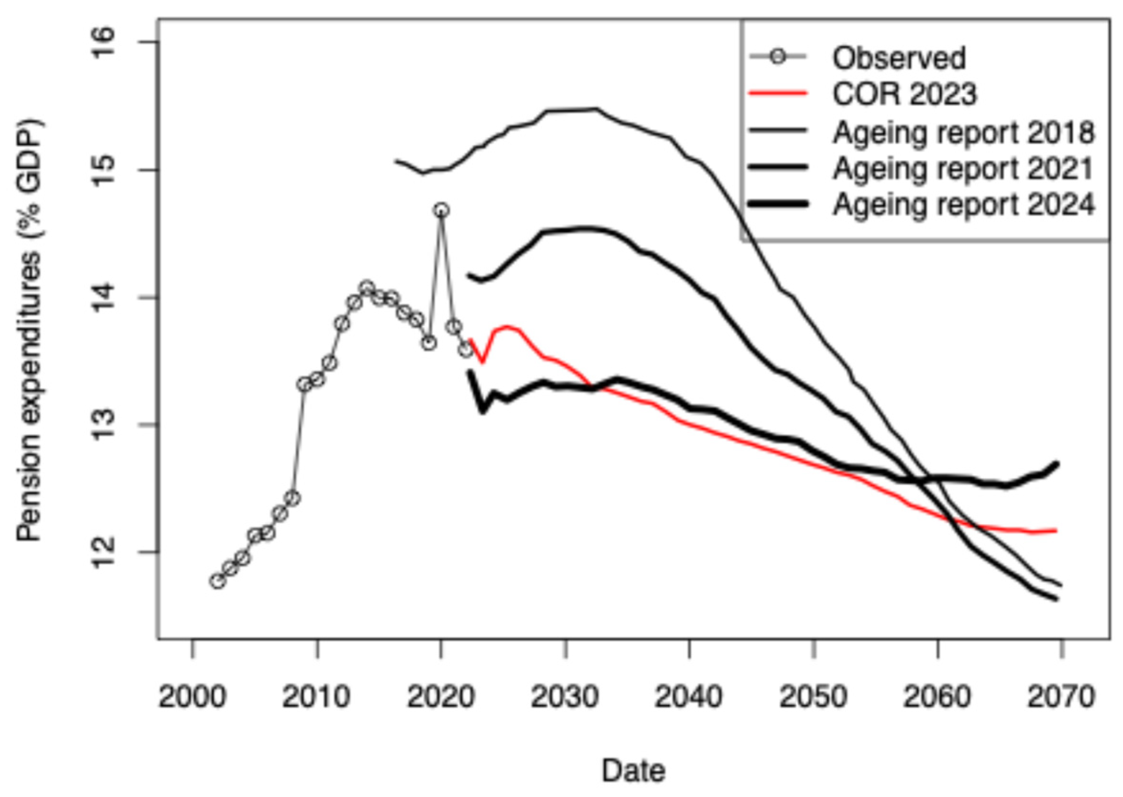
Figure 2. Four main spending trends from scenarios based on productivity scenarios. The expenses are expressed as percentages of GDP. For reference, the expected GDP in 2024 and 2027 are equal to 2588.5 and 4094.1 bn euros, respectively. Observed expenditures are shown using black dots.

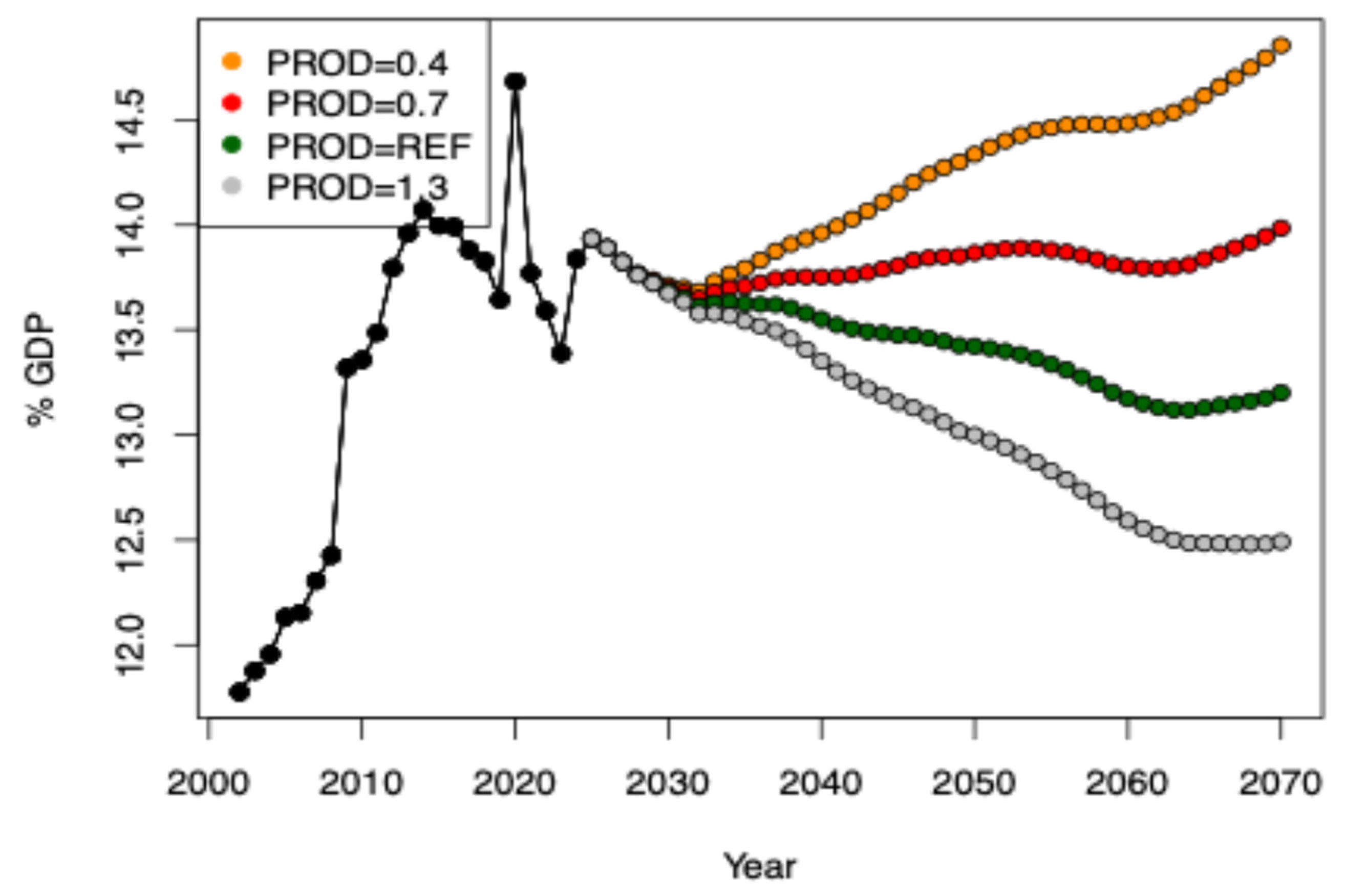
Figure 4. Pension expenditures expressed in % of GDP as a function of Productivity and Life expectancy at 65 for women and men. For reference the data of the year 2020 have been removed from the original dataset. Only one scenario (productivity at 0.4%) shows a positive relationship between GDP and expenditures.

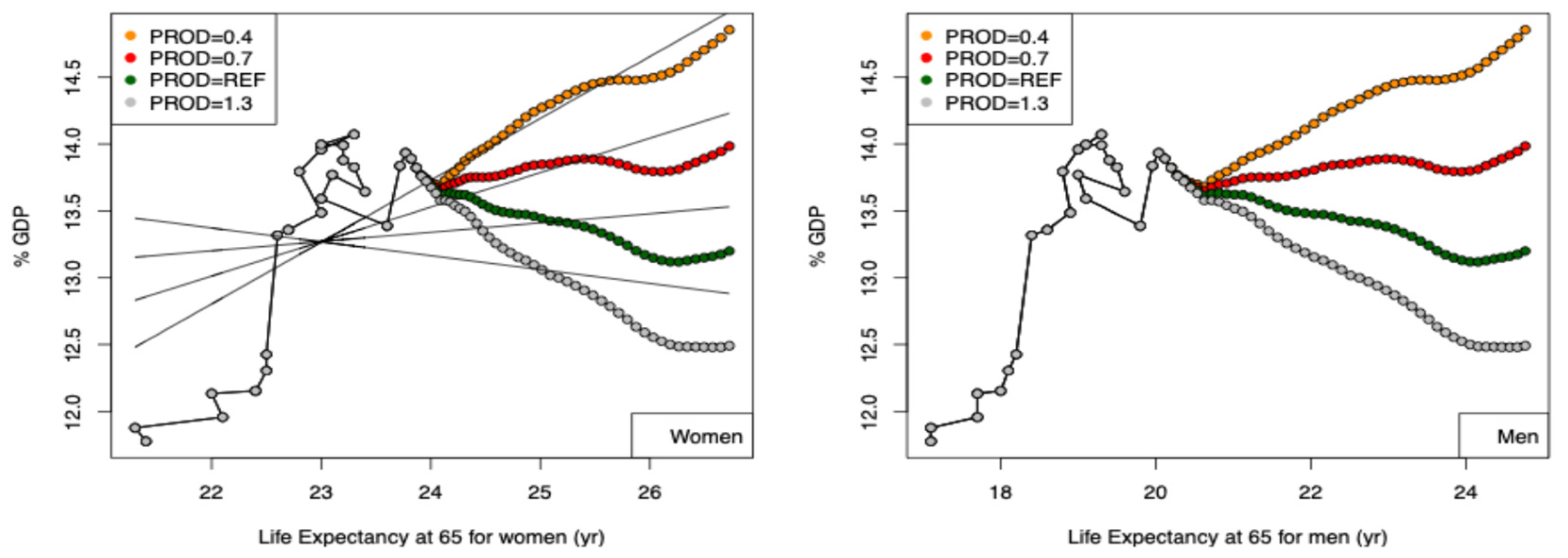
Figure 5. Results for the linear models. Recovered variables are indicated in Table 2 and Table 3. For the first model, standard deviation of values (N=68) equals to 0.13 and RMS = 8.10^-14.

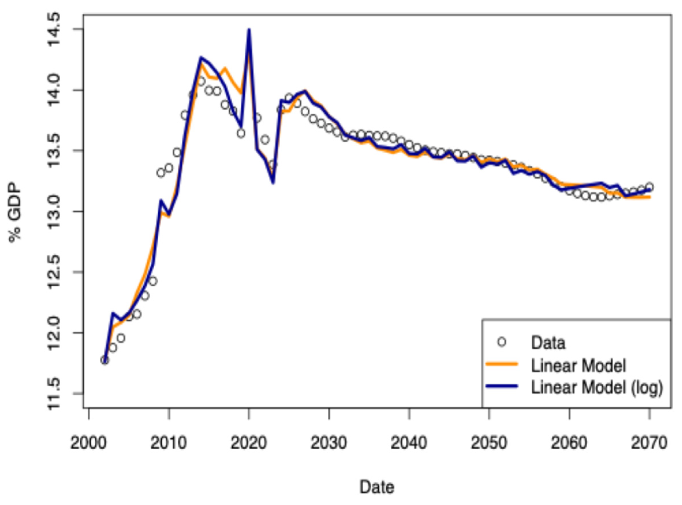
Figure 7. Training results for the four models resulting from the four productivity scenarios. The boundaries are the same as those used in the previous figure. N = 1000 tests for each method with 75% train-test ratio.

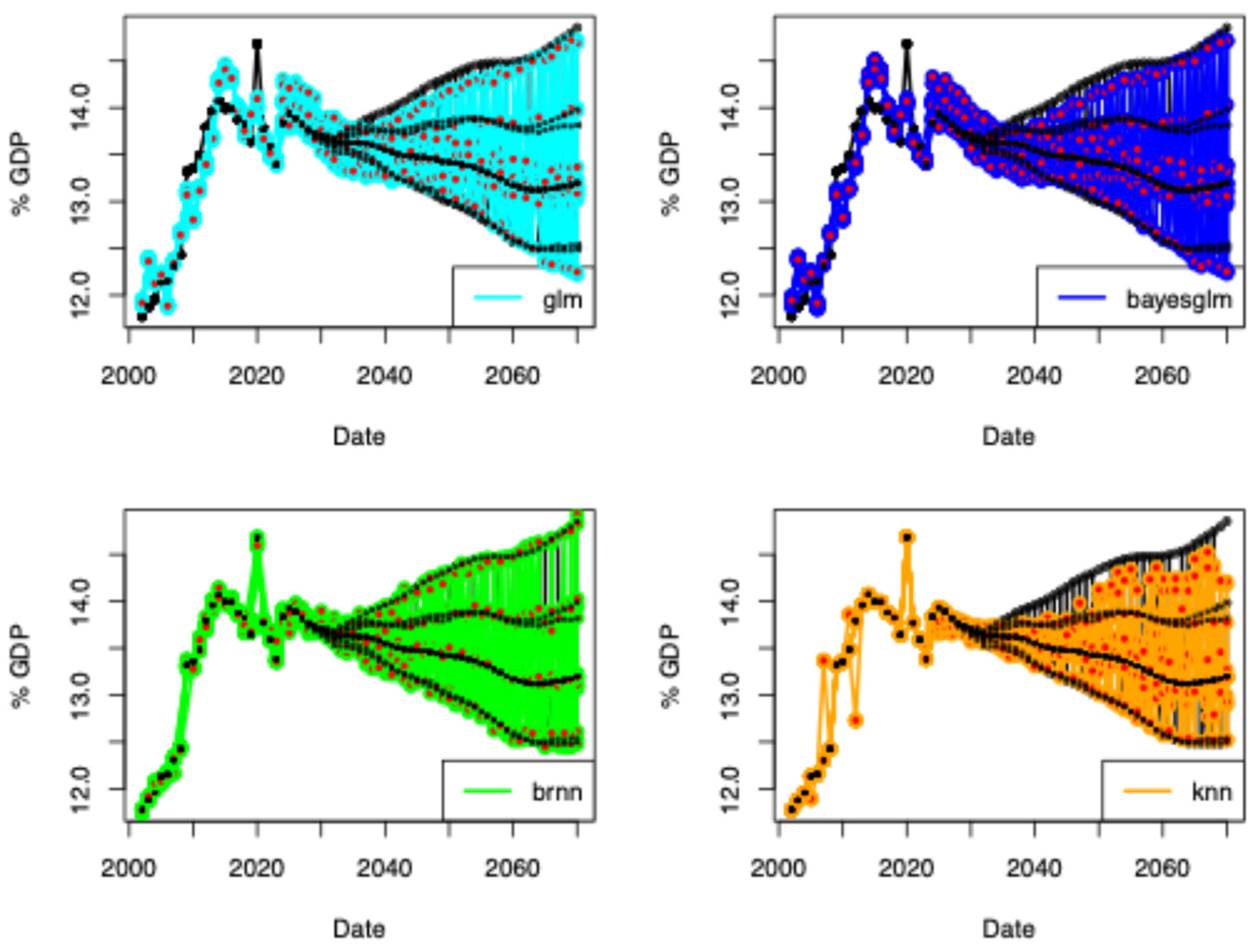
Figure 8. Sensitivity of the pension expenses (“bayesian glm” method) to the variables GDP_VOL, GDP_VAL, ESP_H, and ESP_F for the dataset based on the reference COR scenario.

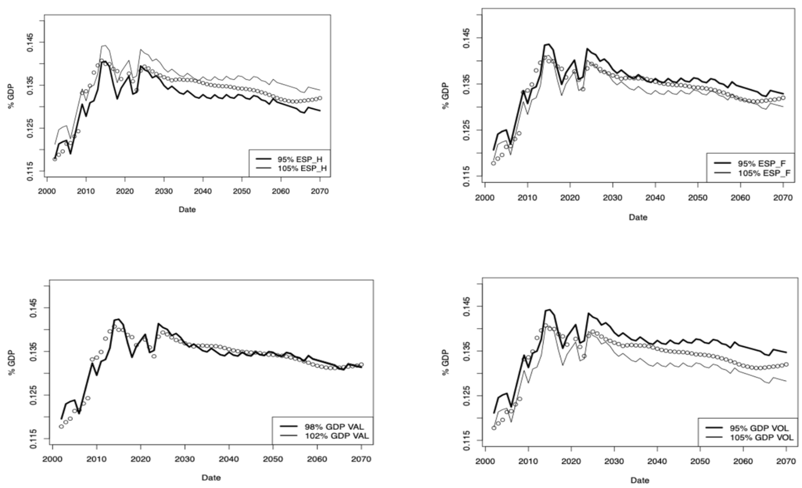
Figure 9. Two models using 4 variables to estimate the pension expenditures. Those models are using only the GDPs (value and volume) and Life expectancy at 65 time-series. For the model using older data (red curve), those variables are either extrapolated using polynoms of order 3 (GDP in volume and LE@65s) or used directly when available (GDP in value). The scattering of differences between the model that include data wrt to the reference COR model, is close +/- 0.3% GDP.

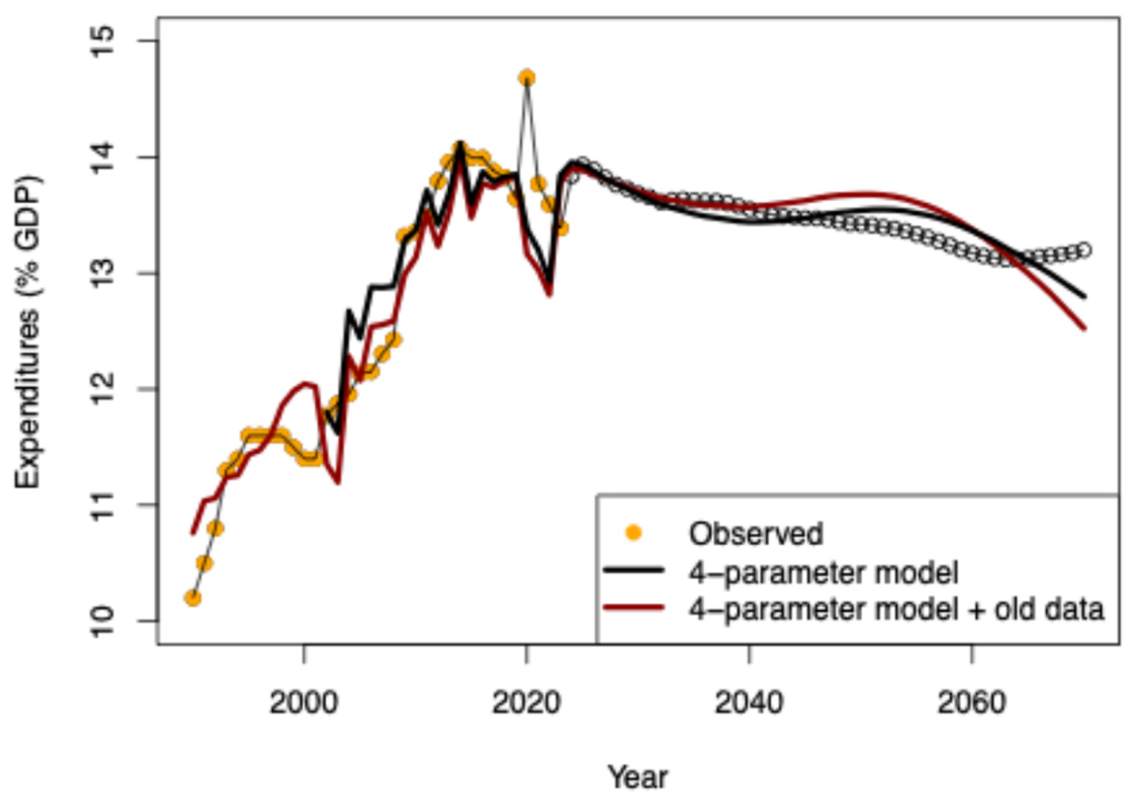
Table 1. Correlation coefficients between Expenses (% GDP) and life expectancy for women and men in the COR main scenarios. There is only a dependency on life expectancy for the most pessimistic scenarios (productivity progression < 1%). For reference, the productivity value within the 2024 European exercise on pension plans equals 1.3% (down from 1.5%).

Scenario Productivity (%)	Life Expectancy at 65 women	Life Expectancy at 65 men
0.4	0.85	0.83
0.7	0.60	0.57
1.0 (Reference)	0.13	0.10
1.3	-0.26	-0.30

Table 2. Results of the linear regression model for main variables considered in this study. The complete formula used in R is shown below⁵. Intercept = -2.80.10^-02.

Productivity	PIB_VOL	GDP_in_value	Life_Expectancy_at_65_women	State_contribution
-6.898e-02	-3.408e-05	1.360e-06	-1.159e-03	4.083e-03
Social_contribution	Migration_count	Unemployment_rate	Life_Expectancy_at_65_men	Fecondity
7.415e-03	9.244e-09	-2.257e-01	1.703e-02	3.313e-02

Table 3. Results of the linear regression model for main variables considered in this study. The complete formula used in R is shown below ⁶. Intercept = 0.484.

Productivity	PIB_VOL	GDP_in_value	Life_Expectancy_at_65_women	State_contribution
-5.097e-04	-0.1753943	0.0379265	-0.2406765	0.0195727
Social_contribution	Migration_count	Unemployment_rate	Life_Expectancy_at_65_men	Fecondity
0.1155438	0.0006357	-0.0150747	0.3328995	0.0613256

Table 4. Variable importances of four models trained on the four COR scenarios datasets. For scenarios with less productivity (0.4 and 0.7) social cost are the most efficient way of changing the impact of pension in % GDP. While productivity is increased, social contribution importance is decreased, and GDP and life expectancy contributions are increased. This test does not show the polarity of the impact of each variable on the output computed. The method used is here Bayesian GLM (blue curves on Figure 6). Variables indicated in bold font are those which showed negative correlations with expenditures in the log-normal model shown in Figure 5 and Table 3.

PROD = 0.4		PROD = 0.7		PROD = REF (1.0)		PROD = 1.3
Social contribution	100	Social contribution	100.0	GDP val	100	LE@65 men	100
LE@65 men	88.1	LE@65 men	94.3	LE@65 men	96.6	LE@65 women	95.5
LE@65 women	79.7	LE@65 women	87.8	LE@65 women	95.9	GDP vol	93.8
GDP vol	73.7	GDP vol	81.9	GDP vol	92.3	GDP val	85.9
GDP val	60.3	GDP val	72.9	Social contribution	71.3	Social contribution	71.8
Migration	29.5	Productivity	33.6	State contribution	14.3	Migration	66.4
Unemployment rate	28.0	State contribution	30.7	Unemployment rate	8.0	Unemployment rate	52.9
Productivity	16.2	Unemployment rate	29.2	Migration	2.5	State contribution	49.2
State contribution	2.3	Migration	5.2	Productivity	1.6	Productivity	45.0
Birth rate	0	Birth rate	0	Birth rate	0	Birth rate	0

Table 6. Six scenarios presented in the study. For all models, the variations are applied to the reference model (productivity rate of 1%).

	Scenario	Modification 1	GDP (Volume)	GDP (Value)
1	Negative Prod. shock plus inflation		-5% over 15 yrs then 0%	+ 5% over 15 years then -5%
2	Positive Prod. shock plus deflation		+5 % over 15 years then +0%	-2% over 15 years then +5%
3	Life expectancy stagnate	LE stagnates from 2040	No change	No change
4	Migration is lower	100’000 per year from 2035	No Change	No change
5	Growth led by migration	150’000 per year from 2035 (stable)	+5 % over 15 years then 0% in growth	No change
6	“Closing the borders”	20’000 per year from 2029	-5% over 15 yrs then 0% in growth	No change

Table 7. Global GDP losses (%) from chronic physical risk by 2050 under various scenarios, according to the Network for Greening the Financial System (NGFS). All GDP losses have been distributed from 2030 to 2050. Progression of GDP have been then matched with COR central scenario. Source: • *Delayed and divergent climate policy response among countries, leading to high physical and transition risks. **Assumes no additional climate policies are implemented until 2030 // https://www.ft.com/content/c00c13a0-492d-40dd-91e7-61d8a1910f6b.

	Scenario	Latest estimate	Previous estimate
A	Current policies	-14.8	-5.4
B	Fragmented world*	-12.9	-5.1
C	Paris Agreement targets	-11.8	-2.9
D	Delayed transitions**	-10.8	-2.8
E	Warming limited to 2degrees	-10.1	-2.6
F	Net Zero by 2050	-7.3	-1.9

Notes

1	A similar recourse to VAT financing has been voted by the Swiss population for financing the “first pilar” of the pension system.
2	https://www.ined.fr/fr/tout-savoir-population/chiffres/projections-mondiales/projections-par-pays/.
3	Eurostat: 2024 Ageing Report France – Country Fiche, Economic Policy Committee – Ageing Working Group, 15 december 2023, Ministry of Economy and Finance, French Treasury.
4	The data were normalized using the following formula: norm(a) = (a-min(a)) / (max(a)-min(a))
5	lm(D_PIB ~ PIB_VOL + GDP_in_value + Productivity + Life_Expectancy_at_65_women + Life_Expectancy_at_65_men + Social_contribution + State_contribution + Migration_count + Fecondity + Unemployment_rate, data = (dataset_COR_REF[,2:12]) )
6	lm(D_PIB ~ PIB_VOL + GDP_in_value + Productivity + Life_Expectancy_at_65_women + Life_Expectancy_at_65_men + Social_contribution + State_contribution + Migration_count + Fecondity + Unemployment_rate, data = log (dataset_COR_REF[,2:12]) )
7	Assuming the pension system is equal to 13% of the 2500 bn GDP and 20% of those savings are reinvested at 1.5% per year, the current return obtained from banks on these deposits is close to 1bn EUR per year. (2’500 bn of GDP/yr * 13% (average expenditures wrt GDP) * 20% (saving rate) * 1.5% (return on investment)= 975 million/yr return on new deposits). For reference, BNP made 11.2bn net income in 2023.
8	Migration and asylum in Europe – 2024 edition https://ec.europa.eu/eurostat/web/interactive-publications/migration-2024#about-this-publication, Catalogue number: KS-FW-24-005-EN-Q ISBN 978-92-68-19608-3 ISSN 2600-3368 doi:10.2785/43971

Disclaimer/Publisher’s Note: The statements, opinions and data contained in all publications are solely those of the individual author(s) and contributor(s) and not of MDPI and/or the editor(s). MDPI and/or the editor(s) disclaim responsibility for any injury to people or property resulting from any ideas, methods, instructions or products referred to in the content.

© 2025 by the authors. Licensee MDPI, Basel, Switzerland. This article is an open access article distributed under the terms and conditions of the Creative Commons Attribution (CC BY) license (http://creativecommons.org/licenses/by/4.0/).

Copyright: This open access article is published under a Creative Commons CC BY 4.0 license, which permit the free download, distribution, and reuse, provided that the author and preprint are cited in any reuse.