
Submitted:
12 December 2025
Posted:
12 December 2025
You are already at the latest version
Abstract
The Discrete Element Method is widely used in applied mechanics, particularly in situations where material continuity breaks down (fracturing, crushing, friction, granular flow) and classical rheological models fail (phase transition between solid and granular). In this study, the Discrete Element Method was employed to simulate stick-slip cycles, i.e., numerical earthquakes. At 2,000 selected, regularly spaced time checkpoints, parameters describing the average state of all particles forming the numerical fault were recorded. These parameters were related to the average velocity of the particles and were treated as the numerical equivalent of (pseudo) acoustic emission. The collected datasets were used to train the Random Forest and Deep Learning models, which successfully predicted the time to failure, also for entire data sequences. Notably, these predictions did not rely on the history of previous stick-slip events. SHapley Additive exPlanations (SHAP) was used to quantify the contribution of individual physical parameters of the particles to the prediction results.
Keywords:
machine learning
; discrete element method
; granular fault gouge
; numerical earthquakes
1. Introduction
Earthquakes are extremely complex geophysical phenomena. Despite decades of research, the processes governing earthquake initiation remain only partially understood. To date, no universal principle has been developed that would allow reliable prediction of the time and magnitude of future seismic events [1]. Short-term deterministic earthquake prediction is currently considered impossible. The general pattern of earthquake occurrence can, however, be described by stick–slip cycles [2]: periods of stress accumulation (stick) are followed by abrupt stress release (slip), reflecting the fundamental dynamics of seismic events.
Among the methods aimed at advancing the understanding of seismic phenomena, acoustic emission (AE) plays a particularly important role. AE can provide insight into processes occurring within fault zones. However, the relationship between acoustic energy and failure in the fault zone remains insufficiently understood. AE arises from material deformation and microcracking, releasing energy that propagates through the material as elastic waves. Owing to its versatility and non-destructive nature, AE is widely used for continuous real-time monitoring of fracture processes.
A major difficulty in earthquake physics research is the lack of sufficient direct observational data, since access to fault zones is limited. Laboratory experiments and numerical simulations can partially address this issue. In modeling failure processes, the Discrete Element Method (DEM) is particularly useful, as it enables tracking the motion of individual particles, interparticle forces, and process dynamics [3]. However, numerical simulations, especially those based on DEM, generate extensive datasets. Machine learning algorithms can effectively analyze such data, identifying hidden linear and nonlinear relationships, and opening new perspectives for earthquake research.
In several recent years, some studies have explored laboratory and numerical investigations of earthquakes, often combining acoustic emission analysis with machine learning techniques. A pioneering study by [4] demonstrated, using laboratory earthquake models, that supervised machine-learning algorithms trained on acoustic signals from stick–slip cycles can accurately predict the timing of subsequent slips. It was confirmed [5] that acoustic emission enables the prediction of both the timing and magnitude of laboratory earthquakes. Supervised learning methods have also contributed to the development of next-generation high-quality earthquake catalogs [6,7]. The Discrete Element Method was employed to predict macroscopic friction based on signals from individual particles [8]. In [9], it was showed that laboratory stick–slip shear experiments replicate the dynamics of natural earthquakes. When sufficient fault dynamics data are available, LightGBM, together with the SHAP value approach, was capable of accurately predicting the friction state of laboratory faults and the most critical input features for laboratory earthquake prediction [10]. Machine learning was also used [11] to show that statistical features of plate motion signals contain information about the slip duration and friction drop of laboratory earthquakes. The Isolation Forest algorithm from unsupervised machine learning was able to detect anomalies [12] in the numerical DEM model of stick-slip cycles. A DEM model was proposed [13] that takes into account an irregular, random pattern of stress increase and decrease in such a system to predict subsequent stick-slip events. In [14], an advanced machine learning was applied to meter-scale laboratory data and demonstrated that a trained model, using a network representation of the event catalog, can accurately predict the time to failure of mainshocks, from tens of seconds to milliseconds before occurrence.
This work is a continuation and complement to the work mentioned above. Here, is presented a DEM model that reproduces stick-slip cycles, hereinafter referred to as numerical earthquakes. Based on continuous (pseudo) acoustic emission monitoring, machine learning models - Random Forest and Deep Learning - were trained. The main goal was to predict the time to failure between successive numerical earthquakes.
2. Materials and Methods
2.1. Discrete Element Method
A fault model capable of reproducing stick–slip cycles was developed. Its construction employed the DEM introduced by [3]. DEM is a particle-based numerical approach used to simulate brittle and granular materials, in which the material is represented as an assembly of interacting discrete elements. The method enables analysis of the translation and rotation of each particle at every time step, where translational motion is governed by Newton’s equations of motion, integrated using a conventional molecular dynamics scheme. The number of particles depends on the model geometry and the packing algorithm, in which larger particles are placed first, and smaller ones subsequently fill the remaining voids. DEM models allow investigation of processes inaccessible to laboratory observation, providing detailed information on each particle throughout the simulation.
The general workflow of a DEM simulation involves preparing the model geometry, followed by execution of the program’s main computational loop. At each iteration, particle contacts are detected, interparticle forces and resulting displacements are computed, and the geometry is updated. This cycle repeats until the simulation is completed. At every time step, Newton’s second law is applied to all discrete elements to compute position and velocity changes induced by acting forces. Numerical stability is satisfied by the Courant time-step criterion [15,16], to have particle displacements sufficiently small. DEM is computationally demanding, and modeling complex phenomena requires simplifications to achieve reasonable computation times [17].
2.2. Numerical Model of a Fault
The proposed model measured 10 × 10 × 1 cm and consisted of 2,465 particles subjected to frictional interactions (Figure 1). Periodic boundary conditions were applied along the x-axis. The model was divided into horizontal layers with different properties, schematically representing the real fault structure [22]. The uppermost and lowermost layers represented undeformed host rock and consisted of particles with a radius of 0.2 cm. Two intermediate layers, representing damaged host rock, contained particles with radii from 0.1 to 0.3 cm. At the model center, a granular layer composed of particles with radii between 0.05 and 0.1 cm was introduced. Other researchers have employed DEM or FDEM fault models of comparable size [8,22,23].
The model was bounded at the top and bottom by rigid walls. A compressive force was applied along the y-axis, and a shear force acted along the x-axis. The simulation consisted of 200,000 time steps. The following unit system was adopted: length unit l = 1 cm, force unit F = 1 mN, and time unit t = 0.01 s. From these base units, derived quantities were defined: velocity v = l/t = 100 cm/s and mass m = 0.01 g.
Mature faults typically contain a granular layer formed by frictional wear and rock fragmentation. This layer significantly affects fault dynamics, stress distribution, and energy release processes [22,24,25]. Therefore, its presence was incorporated into the model.
Due to the high computational cost, the developed model is a simplified representation of a natural fault. Previous studies have shown that stick–slip phenomena in both experimental and numerical models follow the Gutenberg–Richter law and exhibit comparable b-values [24,26]. Furthermore, [27,28] demonstrated that earthquakes exhibit fractal characteristics, meaning that processes occurring at millimeter and centimeter scales are similar to those at meter and kilometer scales [29]. This justifies the use of small-scale laboratory and numerical models in earthquake research.
In fault zones, the grain-size distribution typically follows a power-law relationship, with a small number of large particles and a large number of smaller ones [30]. The presented DEM model exhibits a grain-size distribution within its internal layers comparable to that observed in natural fault zones (Figure 2).
2.3. Machine Learning
Supervised Machine Learning and Deep Learning are widely applied to regression tasks. Classical supervised machine learning algorithms are effective for small- to medium-sized structured datasets, offering low computational cost. In contrast, DL models perform better on large, complex datasets, and their interpretability is more challenging. In the present study, the performance of both approaches was tested in a regression problem.
2.4. Supervised Machine Learning – Random Forest
Supervised machine learning algorithm Random Forest (RF) was applied. RF was validated in similar studies [8,13,14]. RF consists of an ensemble of independent decision trees whose combined output forms the final prediction, applicable to both regression and classification tasks. By aggregating multiple trees, RF mitigates bias and overfitting typical of individual models. As an ensemble learning method, RF employs bootstrap aggregating (bagging), where multiple bootstrap samples are drawn with replacement from the original dataset. Each tree is trained independently. The final prediction is obtained by averaging individual tree outputs (for regression) or majority voting (for classification). Feature randomness further enhances model robustness. Effective RF performance requires tree independence, sufficient data diversity, and balanced tree depth. The algorithm tolerates randomly distributed noise but is sensitive to systematic errors. Although computationally slower and less interpretable than a single decision tree, RF substantially reduces overfitting, producing lower variance and prediction error. In this study, a Random Forest Regressor was implemented, and it constructed 500 regression trees using bagging with random feature selection at each split (max_features=“auto”), a fixed random seed (random_state=42) for reproducibility, and parallel training (n_jobs=-1) to utilize all CPU cores.
2.5. Deep Learning
A Deep Learning (DL) model was implemented using the Keras Sequential API [31,32,33], which represents a strictly feed-forward architecture where layers are stacked linearly, and data flow proceeds from the first layer to the last without branching or skip connections. Sequential models are particularly suitable for tabular regression tasks in which fully connected (dense) layers are sufficient to model nonlinear interactions between variables. The network consisted of two hidden layers with 64 neurons each, using the ReLU activation function to introduce nonlinearity and mitigate vanishing gradient effects. The output layer contained a single linear neuron to match the continuous nature of the regression target. Optimization was performed using the Adam algorithm with default hyperparameters, minimizing the mean squared error (MSE) loss. The network was trained for 120 epochs with a batch size of 32, using a 20% validation split. All input features were standardized via normalization (StandardScaler), ensuring stable gradient propagation and improving convergence.
2.6. Model Training and Testing
Some algorithms are sensitive to differences in feature magnitude and therefore require preprocessing through normalization or standardization, like DL. In contrast, tree-based models such as RF are inherently scale-invariant, eliminating the need for feature scaling. The dataset was divided into a training dataset (80%) and a testing dataset (20%); the model was trained on the training dataset to learn data relationships and evaluated on the testing dataset to assess predictive performance. To further minimize the risk of underfitting or overfitting, K-Fold Cross-Validation was applied, in which the dataset is partitioned into K folds (5-Fold in this case). Each fold serves once as a validation set, while the remaining folds are used for training. Model performance in the regression task was assessed using three standard metrics: the Coefficient of Determination (R2), Mean Absolute Error (MAE), and Mean Squared Error (MSE).
2.7. SHAP
The influence of input features on the target variable was analyzed using SHapley Additive exPlanations (SHAP), a unified framework for model interpretability based on Shapley values from cooperative game theory [34]. SHAP quantifies the contribution of each feature to a model’s prediction, providing consistent additive explanations at both the local (individual prediction) and global (overall feature importance) levels. For tree-based models such as Random Forests, the TreeSHAP implementation enables fast and exact computation of Shapley values, making SHAP an effective method for interpreting complex ensemble models.
3. Results
3.1. Detailed Simulation Settings
Four experiments were carried out: Experiment 1 (E1), Experiment 2 (E2), Experiment 3 (E3), and Experiment 4 (E4). The same DEM model described above was employed in each case. A Normal Confining Force (NFC) of 0.4 mN was applied, and the Shearing Velocity (SV) was set to 2 cm/s. The thickness of the granular layer was 0.5 cm. Each experiment used a different particle density: E1 – 2.6 g/cm3 (2600 kg/m3), E2 – 2.7 g/cm3 (2700 kg/m3), E3 – 2.8 g/cm3 (2800 kg/m3), and E4 – 2.9 g/cm3 (2900 kg/m3). These densities are comparable to those of typical crustal rocks. In each simulation, the Macroscopic Friction Coefficient (MFC) was measured. The dimensionless MFC was defined as the ratio of the shear force [mN] to the normal force [mN] at each simulation time step. The final, average MFC value (aMFC) was obtained as the mean of all MFC values recorded after the consolidation phase (Figure 3). Although density does not directly affect the friction coefficient, it may exert an indirect influence through its impact on mechanical properties. By varying the density values across the four experiments, distinct MFC curve patterns were obtained during the simulations (Figure 3). Data collected during each simulation was used for training and testing machine learning algorithms. Each simulation comprised 200,000 time steps. The time step values were as follows: E1 – t1 = 0.0000213 s; E2 – t2 = 0.0000217 s; E3 – t3 = 0.0000221 s; and E4 – t4 = 0.0000225 s. The total simulated durations were: E1 – 4.26 s; E2 – 4.34 s; E3 – 4.42 s; and E4 – 4.50 s.
3.2. MFC Curves During Stick-Slip Cycles
During the simulation (Figure 3), both the NFC and the SV were initially set to zero. The NFC increased linearly from 0 to the target value of 0.4 N over the time-step interval 0–5,000, representing the consolidation period. Thereafter, NFC remained constant until the end of the simulation. The SV increased from 0 to 2 cm/s between time steps 30,000 and 40,000, following the so-called ramp protocol, and then remained constant for the remainder of the simulation. The MFC was computed at each time step. For each simulation, aMFC was calculated only after the consolidation period and ramp protocol, that is, for the time-step interval 50,000–200,000, referred to as the Simulation Interval (SI). The following aMFC values were obtained (Figure 3): E1 – aMFC = 0.8006; E2 – aMFC = 0.7914; E3 – aMFC = 0.8069; and E4 – aMFC = 0.8009.
The data used for training and testing the machine learning algorithms were collected over the same time-step interval SI. The objective of applying machine learning algorithms was to predict the Time to Failure (TtF). The TtF was determined based on the first derivative of MFC within SI. Increases in MFC values were interpreted as the stick phase, whereas decreases corresponded to the slip phase. The TtF was defined as the time between consecutive sign changes of the first derivative from negative to positive—that is, the moment when MFC stopped decreasing and began to increase. This transition corresponds to the end of a slip phase and the start of a stick phase. Each interval between two successive changes in the derivative’s sign from negative to positive was treated as an individual numerical earthquake event. The duration of the slip phase was assumed to be relatively short compared to the stick phase; therefore, the TtF was measured from the beginning of the stick phase to the end of the subsequent slip phase.
3.3. (Pseudo) Acoustic Emission
As shown in Figure 3, the stick–slip cycles in each experiment exhibited irregular and unique characteristics. The aim was to predict the TtF not based on the history of previous cycles, but through continuous monitoring of the state of particles forming the numerical fault. During the simulation, four parameters were recorded at each time step (Table 1): the mean X component of particle velocity (vx_m), the mean Y component of particle velocity (vy_m), the standard deviation of the X component (vx_std), and the standard deviation of the Y component (vy_std).
Because local variations may not be reflected in mean values, the standard deviation was also included. These parameters were treated as (pseudo) Acoustic Emission (PAE). It was demonstrated [25] that in DEM simulations of stick–slip cycles, PAE can be effectively derived from quantities related to particle velocity.
3.4. Kinetic Energy Changes
The kinetic energy plot (Figure 4) from the four DEM simulations exhibits a characteristic, irregular sequence of peaks with varying amplitudes, typical of stick–slip cycles. The periods of NCF activation, corresponding to time steps 0–5000, are marked with vertical dashed lines. The linear increase in the applied NCF value was accompanied by a proportional rise in kinetic energy. Between time steps 5000 and 30,000, the kinetic energy decreased nearly to zero, as the NCF no longer induced particle motion. In the interval between time steps 30,000 and 40,000, the SV was initiated and increased linearly. After time step 40,000, the main simulation phase commenced. When the system entered stick-slip mode, alternating phases were observed: periods of stopped motion, corresponding to stress accumulation during the stick-slip phase, and sharp, sudden peaks of kinetic energy, corresponding to slip events.
The distribution of peak amplitudes qualitatively resembles the Gutenberg–Richter law, in which small events occur much more frequently than large ones, while occasional extreme values correspond to major events. Overall, the results indicate that the presented numerical model reproduces, in an approximate manner, the key statistical and dynamic characteristics observed in laboratory-scale earthquakes.
3.5. TtF Prediction Methodology
During the simulation, so-called checkpoints were established within the SI at every hundredth time step. This approach, known as the moving time window technique, was used to record PAE at each checkpoint. Data were not collected at every time step in order to avoid excessive data accumulation. In each of the experiments E1–E4, approximately 1 GB of data was collected in total. For comparison, collecting data at every second time step would have resulted in approximately 150 GB per simulation. The collected data were used to train a supervised machine learning algorithm RF and a DL neural network. The parameters (features) associated with PAE were treated as dependent variables, while the TtF was defined as the independent variable. Predictions were made solely based on continuous monitoring of PAE from individual time windows, so the models generated forecasts without utilizing the history of previous events.
Figure 5 compares the MFC within the SI for each experiment with the TtF. The TtF values were normalized with respect to their maximum value to enable direct comparison with the MFC curves.
As shown in Figure 5, after the completion of each numerical earthquake, the TtF curve rises sharply to its maximum value and then gradually decreases as the end of the numerical event approaches.
3.6. Achievements of Machine Learning Algorithms
RF and DL performed very well with the predictions, as shown in Table 2. Results are presented for the training and testing datasets for experiments E1-E4 for the R2, MAE, and MSE metrics. Metrics on the training datraset are given as means with standard deviation, as they were the result of 5-Fold Cross Validation. Very good R2 metrics above 90% were obtained. Experiment E3 was an exception, with a result below 90%. The MAE and MSE metrics had small values, indicating accurate predictions. Overall, RF performed slightly better than DF.
Figure 6 visually presents the predictions of the RF and DL algorithms on the test set. Ideally, all points would fall on the dashed straight line, indicating 100% prediction accuracy. It can be seen that the predictions are clustered close to the ideal prediction line, confirming the very good results of the metrics in Table 2.
The obtained results indicate that both machine learning algorithms, RF and DL, performed very well in predicting outcomes using only features derived from PAE. In most cases, the coefficient of determination (R2) exceeded 90% for both algorithms, on both the training and test datasets.
3.7. Computational Time – Training of RF and DL
DL is an incomparably more powerful tool than supervised machine learning, but it’s often not cost-effective. The actual training times of the RF and DL algorithms were compared (Figure 7). Training efficiency and computational time are important factors in determining which algorithm is more suitable for a given problem. For E1, the training time was 4.23 s for RF and 20.32 s for DL. For E2, the corresponding values were 3.15 s for RF and 21.31 s for DL; for E3, 4.23 s for RF and 21.34 s for DL; and for E4, 2.99 s for RF and 21.54 s for DL.
It was observed that the RF algorithm was approximately five to seven times faster than DL, and it achieved better metrics. In addition, a very simple DL architecture was used here, a more complex one would definitely be more time-consuming. This indicates that DL is highly effective for analyzing large datasets with complex and nonlinear dependencies, but its application to other problems is computationally inefficient. In such cases, supervised machine learning algorithms are more appropriate.
3.8. In-Depth Analysis of the Impact of Features on Predictions with SHAP
In the four configurations (E1–E4), a comparative analysis of the influence of features (independent parameters) was conducted for the Random Forest and Deep Learning using SHAP values (Figure 8). The order of parameters on the y-axis corresponds to their influence on the algorithm’s performance, ordered from highest to lowest. Across all experiments, the same pattern was observed – vx_m had the greatest impact on the performance of both the RF and DL models. In most cases, vx_std had the smallest impact. The second and third most influential parameters were the parameters related to velocity in the y-axis direction, i.e., vy_m and vy_std. Interestingly, this pattern was repeated for both the RF and DL models, despite the completely different characteristics of these models.
Regarding the x-axis of the SHAP plot, if the single data points had a high value (within a given feature), they were marked with a warm color. If they had a low value, then they were marked with a cool color. The position on the x-axis indicated the individual SHAP value calculated for each of the points. The results obtained in E1-E4 demonstrate high similarity, indicating that the observed dependency structure was not an artifact of a specific model architecture or data configuration. For both algorithms, low values of vx_m have a negative impact on model output, but data points are clustered close to the value 0. Conversely, high values of this feature have a high positive impact on model output, but data points are distributed irregularly along the axis. Regarding vy_m, the impact pattern is reversed compared with vx_m: high-value points have a strong negative impact, while low-value points have a strong positive impact. In the case of vx_std and vy_std, generally, small standard deviations give a low positive impact on model output, and high values of standard deviation give a low negative impact on model output.
3.9. Predicting the Entire Numerical Earthquake
In the analyses presented above, the training of the RF and DL algorithms in experiments E1–E4 was based on a random selection of data points for the training and testing datasets. Although this is a standard procedure in machine learning, such an approach does not address whether the trained algorithm is capable of predicting an entire data sequence. In the context of numerical earthquake prediction, the primary objective is to forecast the TtF for an entire event. Therefore, a modified training approach was employed in the next stage of the study. Specifically, 90% of the initial TtF values in each experiment were used for training, while the remaining 10% of the final TtF values were reserved for testing. This approach enabled the algorithms to evaluate their predictive capability across the entire data series, effectively forecasting complete future events. Figure 9 presents a visualization of the prediction results for the last 10% of data points (testing dataset) from a representative segment of the curve. Only RF was used because it performed better for this type of problem than DL, as in Table 2.
The R2 metric for each experiment was several percentage points lower than in Table 2, but overall, very satisfactory results were obtained. RF was able to predict and reproduce the TtF at every time step with satisfactory accuracy. Only in the case of E3 did intermittent predictions appear. These results demonstrate that RF is capable of predicting an entire series of events based on PAE monitoring.
4. Discussion
Scientific work is ongoing to better understand real seismic phenomena. However, at the current state of knowledge, the only earthquakes that can be predicted are those in the laboratory experiments [4,14] and those modeled numerically [8,13]. Machine learning helps in automatically finding patterns and relationships from huge datasets, especially nonlinear relationships. The methodology developed in this way can then be tested in the real world. This work is a continuation of scientific research in this area. A numerical DEM model reproducing stick-slip cycles was proposed. During the four numerical experiments, (pseudo) Acoustic Emission monitoring was carried out. This measurement was intended to detect the time to subsequent numerical earthquakes. Two machine learning approaches - Random Forest and Deep Learning - were applied to learn and identify the relationships between the (pseudo) acoustic signal and the time to the next events.
Main findings and conclusions:
- The present study was based on several simplifying assumptions; however, its objective was to provide a qualitative rather than quantitative description of the investigated phenomenon.
- Very good metrics were achieved on the training and testing datasets, with average R2 exceeding even 95% on training dataset and 97% with R2 exceeding even 97% on testing dataset. Overall, RF performed slightly better than DF.
- Model training times were compared and it turned out that the Random Forest model took up to seven times less time to train than a simple deep learning architecture, yet the Random Forest algorithm had better evaluation metrics on both the training and test sets. This demonstrates that it’s always important to compare different machine learning techniques to find the most efficient ones.
- SHAP analysis of the influence of independent parameters showed that among the four features constituting (pseudo) Acoustic Emission, the average particle velocity in the x-axis direction had the greatest impact on the algorithm’s predictions, both for Random Forest and Deep Learning.
- It has also been shown that the Random Forest algorithm can predict Time To Failure for entire sequences of numerical earthquakes with an R2 statistic of about 90%.
- The results achieved confirm that it is possible to predict earthquakes in numerical and laboratory experiments using machine learning. However, in numerical and laboratory systems, a virtually unlimited amount of data is available about the system being studied. This is what makes machine learning so efficient in such applications. In the case of real-world phenomena, the available data is limited, which limits the possibilities of machine learning.
- However, scientific research under controlled conditions is needed to develop a methodology that can then be verified on real phenomena.
Funding
This research was funded by NCN MINIATURA 6 grant (National Science Centre, Poland), grant number No. DEC-2022/06/X/ST10/01581. The author would also like to thank the statutory funds of the Institute of Geophysics, Polish Academy of Sciences, for their support.
Institutional Review Board Statement
Not applicable.
Data Availability Statement
Code and results are available in the Data Portal of the Institute of Geophysics, Polish Academy of Sciences (IG PAS): − licence: Creative Commons Attribution 4.0 International (CC BY 4.0); − DOI: https://doi.org/10.25171/InstGeoph_PAS_IG-Data_Predictions_of_Numerical_Earthquakes; − link: https://dataportal.igf.edu.pl/dataset/predictions_of_numerical_earthquakes
Acknowledgments
Prof. Guilhem Mollon is thanked for supplying the opportunity of a scientific stay in Lyon in June 2023. The work of the authors of ESyS-Particle Tutorial (Abe et al., 2014) is appreciated. The author would also like to thank the Scientific Information and Publishers Department of IG PAS for the language correction.
Special thanks are due to my Mother, Wiesława Klejment, and Uncle from Gdynia, Jan Domysławski, for their support.
Conflicts of Interest
The authors declare no conflicts of interest. The funders had no role in the design of the study; in the collection, analyses, or interpretation of data; in the writing of the manuscript; or in the decision to publish the results.
Abbreviations
The following abbreviations are used in this manuscript:
| AE | Acoustic Emission |
| DEM | Discrete Element MethodRandom Forest (RF) |
| RF | Random Forest |
| DL | Deep Learning |
| R2 | Coefficient of Determination |
| MAE | Mean Absolute Error |
| MSE | Mean Squared Error |
| SHAP | SHapley Additive exPlanations |
| E1 | Experiment 1 |
| E2 | Experiment 2 |
| E3 | Experiment 3 |
| E4 | Experiment 4 |
| NFC | Normal Confining Force |
| SV | Shearing Velocity |
| MFC | Macroscopic Friction Coefficient |
| aMFC | average Macroscopic Friction Coefficient |
| SI | Simulation Interval |
| TtF | Time to Failure |
| vx_m | mean X component of particle velocity |
| vy_m | mean Y component of particle velocity |
| vx_std | standard deviation of the X component |
| vy_std | standard deviation of the Y component |
| PAE | (pseudo) Acoustic Emission |
References
- Senatorski, P. Sejsmiczność, trzęsienia ziemi i lingwistyka [Seismicity, earthquakes and linguistics]. Przegląd Geofizyczny 2023, 68(3–4), 185–197. [Google Scholar] [CrossRef]
- Brace, W. F.; Byerlee, J. D. Stick-Slip as a Mechanism for Earthquakes. Science 1966, 153(3739), 990–992. [Google Scholar] [CrossRef]
- Cundall, P.A.; Strack, O.D.L. A discrete numerical model for granular assemblies. Geotechnique 1979, 29(1), 47–65. [Google Scholar] [CrossRef]
- Rouet-Leduc, B.; Hulbert, C.; Lubbers, N.; Barros, K.; Humphreys, C. J.; Johnson, P. A. Machine learning predicts laboratory earthquakes. Geophysical Research Letters 2017, 44, 9276–9282. [Google Scholar] [CrossRef]
- Bolton, D. C.; Shreedharan, S.; Rivière, J.; Marone, C. Acoustic energy release during the laboratory seismic cycle: Insights on laboratory earthquake precursors and prediction. Journal of Geophysical Research: Solid Earth 2020, 125, e2019JB018975. [Google Scholar] [CrossRef]
- Beroza, G.C.; Segou, M.; Mostafa Mousavi, S. Machine learning and earthquake forecasting—next steps. Nat Commun 2021, 12, 4761. [Google Scholar] [CrossRef]
- Kubo, H.; Naoi, M; Kano, M. Recent advances in earthquake seismology using machine learning. Earth, Planets and Space 2024, 76, 36. [Google Scholar] [CrossRef]
- Ren, C. X.; Dorostkar, O.; Rouet-Leduc, B.; Hulbert, C.; Strebel, D.; Guyer, R. A.; et al. Machine learning reveals the state of intermittent frictional dynamics in a sheared granular fault. Geophysical Research Letters 2019, 46, 7395–7403. [Google Scholar] [CrossRef]
- Mollon, G.; Aubry, J.; Schubnel, A. Laboratory earthquakes simulations—Typical events, fault damage, and gouge production. Journal of Geophysical Research: Solid Earth 2023, 128, e2022JB025429. [Google Scholar] [CrossRef]
- Huang, W.; Gao, K.; Feng, Y. Predicting Stick-Slips in Sheared Granular Fault Using Machine Learning Optimized Dense Fault Dynamics Data. J. Mar. Sci. Eng. 2024, 12, 246. [Google Scholar] [CrossRef]
- Wei, M.; Gao, K. Machine learning predicts the slip duration and friction drop of laboratory earthquakes in sheared granular fault. Journal of Geophysical Research: Machine Learning and Computation 2024, 1, e2024JH000398. [Google Scholar] [CrossRef]
- Klejment, P. Detecting Anomalies in Numerical Stick-Slip Cycles with the Unsupervised Algorithm Isolation Forest. Przegląd Geofizyczny 2024, vol. 69(iss. 3-4), 115–133. [Google Scholar] [CrossRef]
- Klejment, P. Non-history-based DEM model for predictions of numerical earthquakes. Geology, Geophysics and Environment 2025, vol. 51(3), 255–270. [Google Scholar] [CrossRef]
- Norisugi, R.; Kaneko, Y.; Rouet-Leduc, B. Machine learning predicts meter-scale laboratory earthquakes. Nat Commun 2025, 16, 9593. [Google Scholar] [CrossRef]
- O’Sullivan, C.; Bray, J.D. Selecting a suitable time step for discrete element simulations that use the central difference time integration scheme. Eng. Comput 2004, 21, 2–4, 278–303. [Google Scholar] [CrossRef]
- O’Sullivan, C. Particulate Discrete Element Modelling: A Geomechanics Perspective; Spon Press/Taylor and Francis: London, 2011. [Google Scholar]
- Klejment, P. Application of supervised machine learning as a method for identyfying DEM contact law parameters. Mathematical Biosciences and Engineering 2021, 18(6), 7490–7505. [Google Scholar] [CrossRef] [PubMed]
- Wang, Y.; Abe, S.; Latham, S.; Mora, P. Implementation of Particle-scale Rotation in the 3-D Lattice Solid Model. Pure and Applied Geophysics 2006, 163, 1769–1785. [Google Scholar] [CrossRef]
- Wang, Y.C. A new algorithm to model the dynamics of 3-D bonded rigid bodies with rotations. Acta Geotech 2009, 4(2), 117–127. [Google Scholar] [CrossRef]
- Weatherley, D.K.; Boros, V.E.; Hancock, W.R.; Abe, S. Scaling benchmark of ESyS-Particle for elastic wave propagation simulations. 2010 IEEE Sixth Int. Conf. E-Science, Brisbane, Australia; 2010; pp. 277–283. [Google Scholar] [CrossRef]
- Abe, S.; Boros, V.; Hancock, W.; Weatherley, D. ESyS-particle tutorial and user’s guide, 2014, Version 2.3.1. Available online: https://launchpad.net/esys-particle.
- Ferdowsi, B. Discrete element modeling of triggered slip in faults with granular gouge: Application to dynamic earthquake triggering. PhD thesis, ETH Zürich, 2014. [Google Scholar] [CrossRef]
- Ma, G.; Mei, J.; Gao, K.; Zhao, J.; Zhou, W.; Wang, D. Machine learning bridges microslips and slip avalanches of sheared granular gouges. Earth and Planetary Science Letters 2022, 579, 117366. [Google Scholar] [CrossRef]
- Dorostkar, O. Stick-slip dynamics in dry and fluid saturated granular fault gouge investigated by numerical simulations. Doctoral Thesis, ETH Zurich, 2018. [Google Scholar] [CrossRef]
- Dorostkar, O.; Carmeliet, J. Grain friction controls characteristics of seismic cycle in faults with granular gouge. Journal of Geophysical Research: Solid Earth 2019, 124, 6475–6489. [Google Scholar] [CrossRef]
- Dahmen, K.; Ben-Zion, Y.; Uhl, J. A simple analytic theory for the statistics of avalanches in sheared granular materials. Nature Phys 2011, 7, 554–557. [Google Scholar] [CrossRef]
- Kanamori, H.; Anderson, D. L. Theoretical basis of some empirical relations in seismology. Bull. Seismol. Soc. Am. 1975, 65, 1073–1095. [Google Scholar]
- Prieto, G.A.; Shearer, P.M.; Vernon, F.L.; Kilb, D. Earthquake source scaling and self-similarity estimation from stacking p and s spectra. Journal of Geophysical Research: Solid Earth 2004, 109(B8). [Google Scholar] [CrossRef]
- Rivière, J.; Lv, Z.; Johnson, P.A.; Marone, C. Evolution of b-value during the seismic cycle: Insights from laboratory experiments on simulated faults. Earth and Planetary Science Letters 2018, 482, 407–413. [Google Scholar] [CrossRef]
- Muto, J.; Nakatani, T.; Nishikawa, O.; Nagahama, H. Fractal particle sizedistribution of pulverized fault rocks as afunction of distance from the fault core. Geophys. Res. Lett. 2015, 42, 3811–3819. [Google Scholar] [CrossRef]
- Géron, A. Hands-On Machine Learning with Scikit-Learn, Keras, and TensorFlow, 2nd Edition; O’Reilly Media, Inc., 2019. [Google Scholar]
- Liu, Y.H. Python Machine Learning By Example: Build intelligent systems using Python, TensorFlow 2, PyTorch, and Scikit-Learn, 3rd Edition; Packt Publishing, 2020. [Google Scholar]
- Raschka, S.; Mirjalili, V. Python Machine Learning: Machine Learning and Deep Learning with Python, Scikit-Learn, and TensorFlow 2, 3rd Edition; Packt Publishing, 2019. [Google Scholar]
- Strumbelj, Erik; Kononenko, Igor. Explaining prediction models and individual predictions with feature contributions. Knowledge and information systems 2014, 41.3, 647–665. [Google Scholar] [CrossRef]
Figure 1.
Schematic representation of the DEM numerical model of the fault.
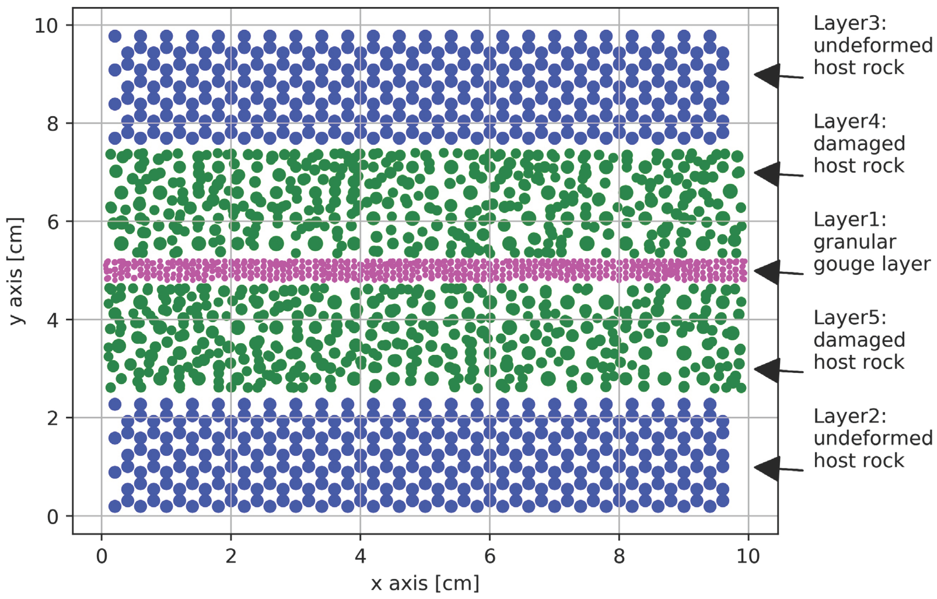
Figure 2.
Particle size distribution in the model following a power-law distribution.
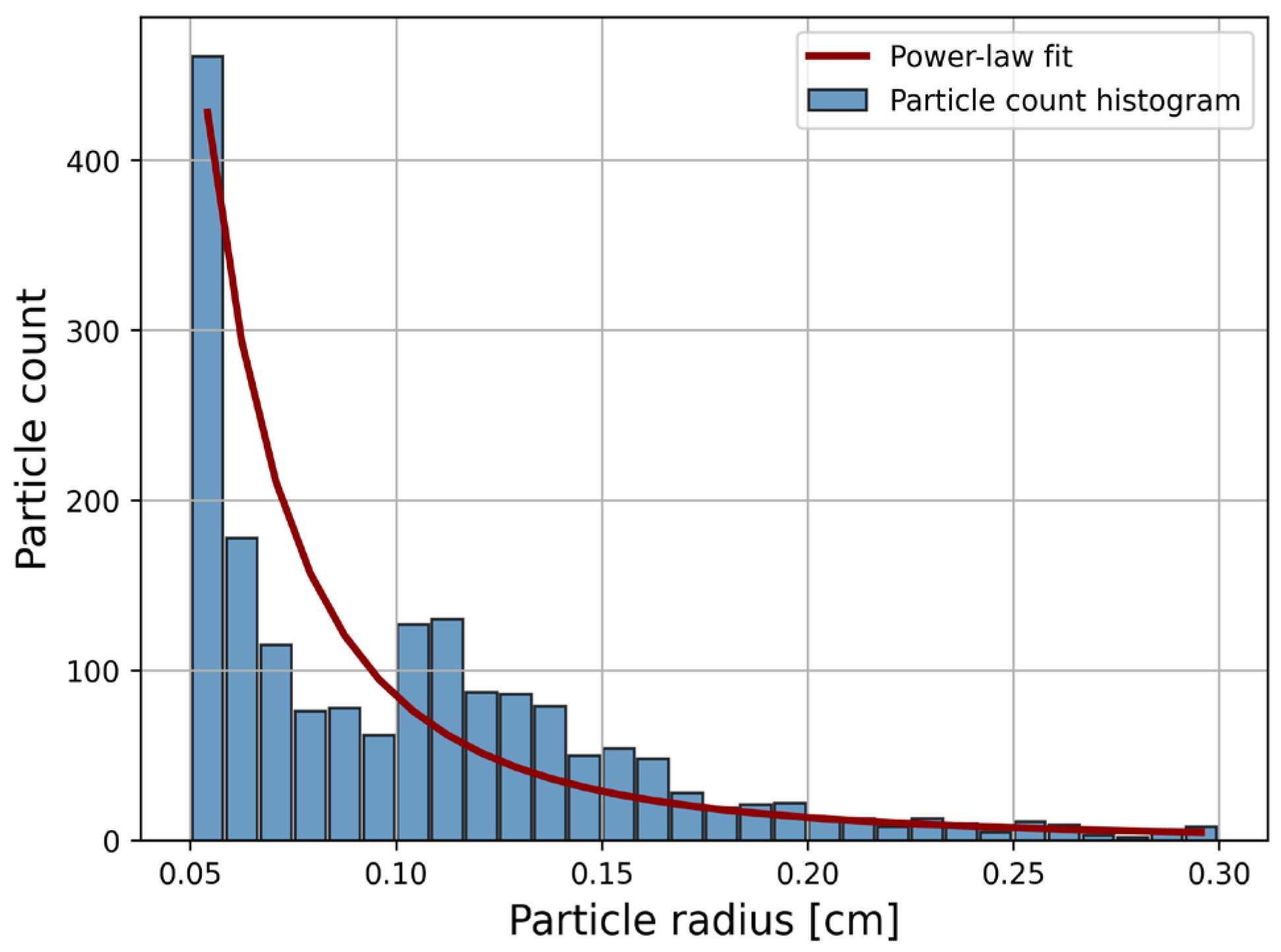
Figure 3.
MFC curves for experiments E1-E4: (a) Experiment 1; (b) Experiment 2; (c) Experiment 3; (d) Experiment 4.
Figure 3.
MFC curves for experiments E1-E4: (a) Experiment 1; (b) Experiment 2; (c) Experiment 3; (d) Experiment 4.
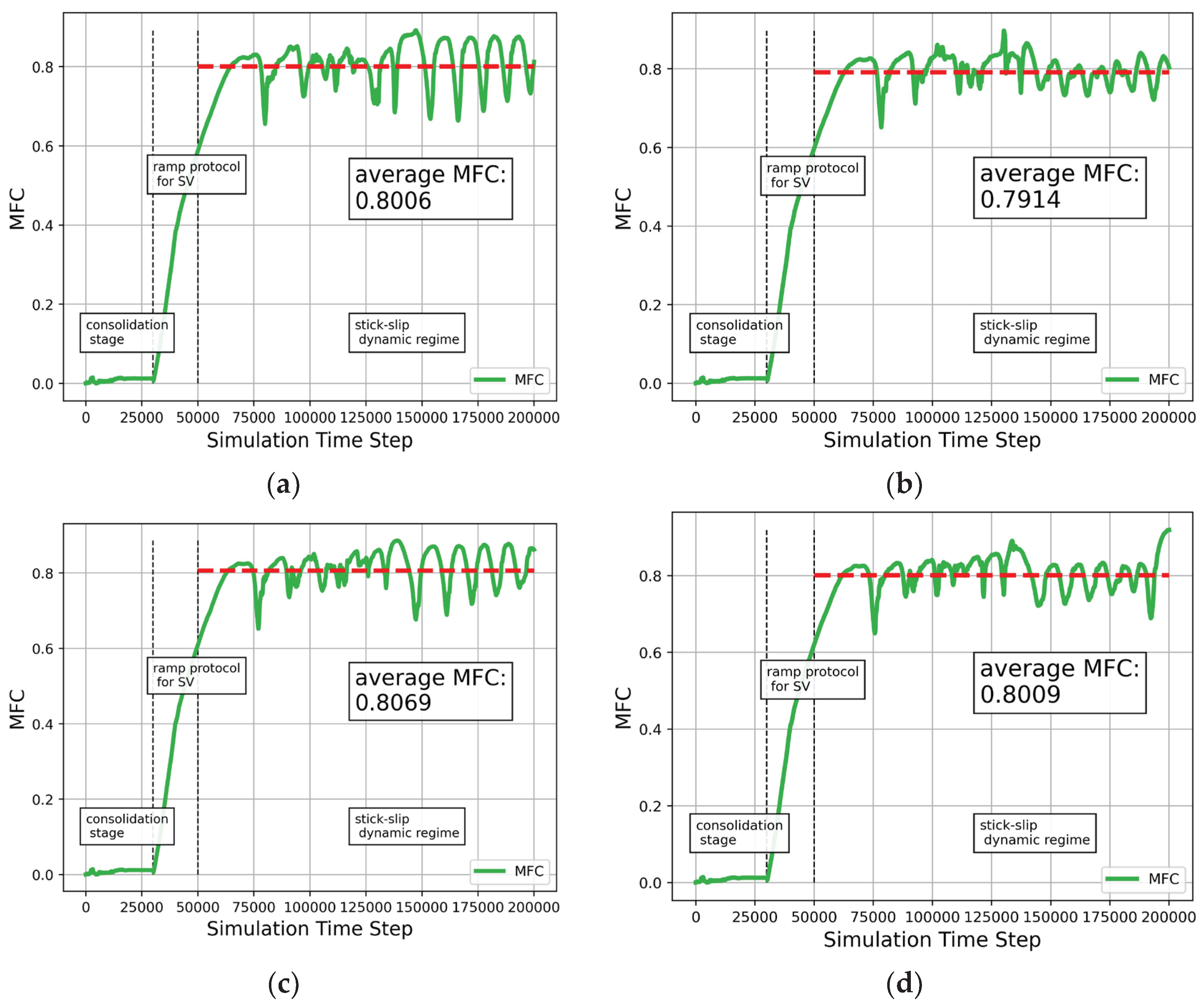
Figure 4.
Kinetic energy for experiments E1-E4.
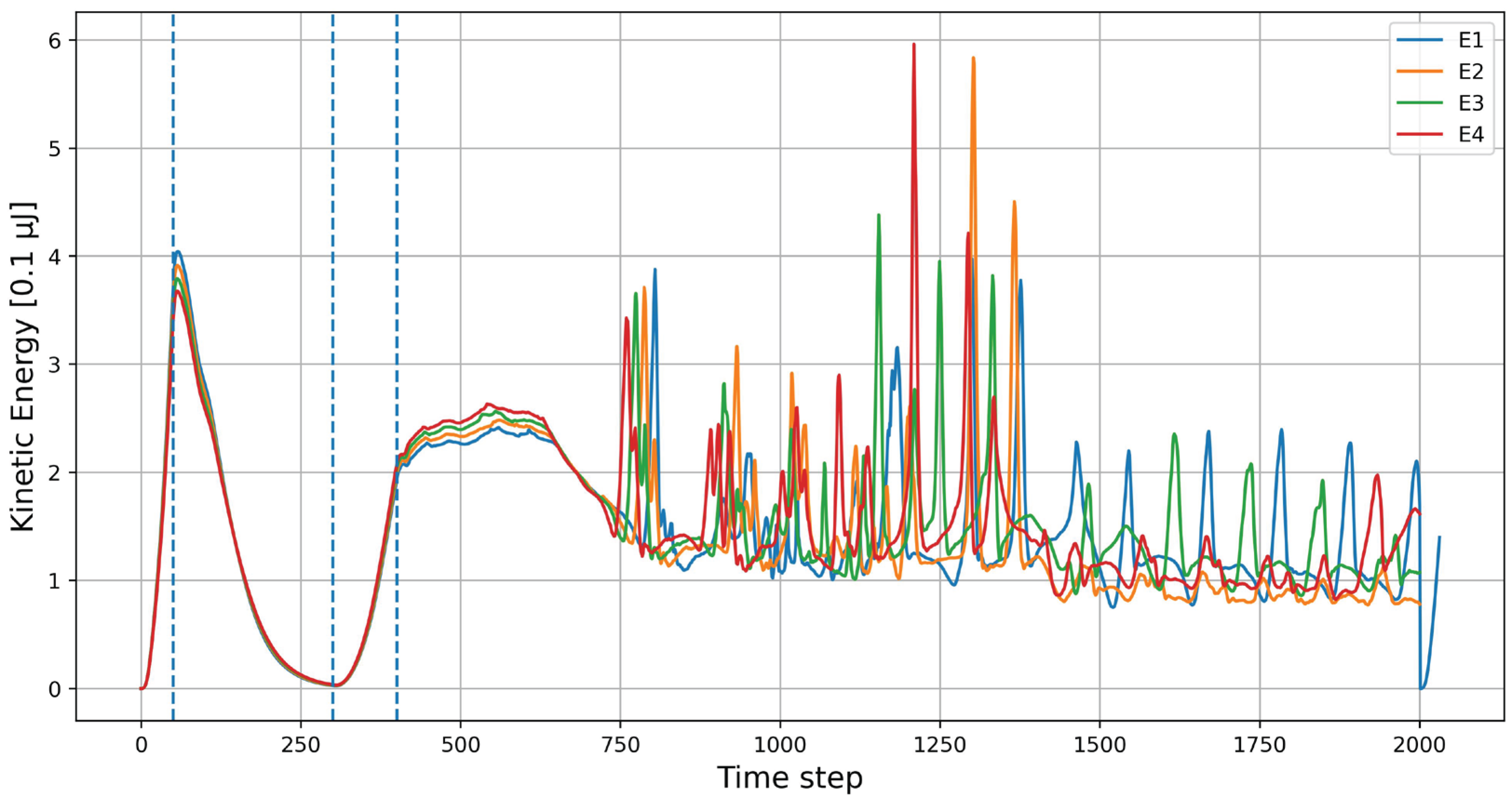
Figure 5.
Comparison between MFC and normalized TtF for: (a) Experiment 1; (b) Experiment 2; (c) Experiment 3; (d) Experiment 4.
Figure 5.
Comparison between MFC and normalized TtF for: (a) Experiment 1; (b) Experiment 2; (c) Experiment 3; (d) Experiment 4.
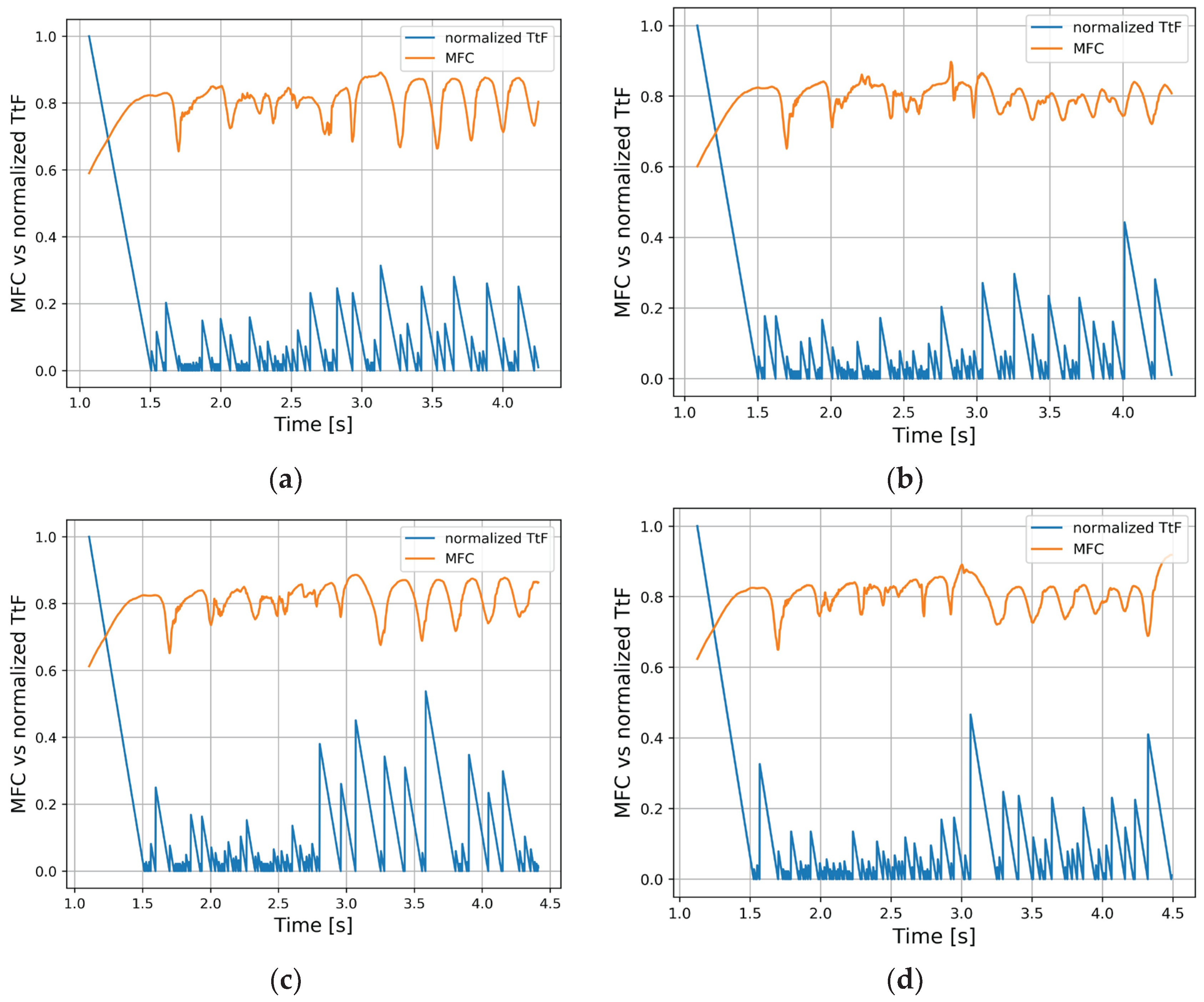
Figure 6.
Real vs Predicted Data on the test dataset for: (a) Experiment 1 – Random Forest; (b) Experiment 1 – Deep Learning; (c) Experiment 2 – Random Forest; (d) Experiment 2 – Random Forest; (e) Experiment 3 – Random Forest; (f) Experiment 3 – Random Forest; (g) Experiment 4 – Random Forest; (h) Experiment 4 – Random Forest.
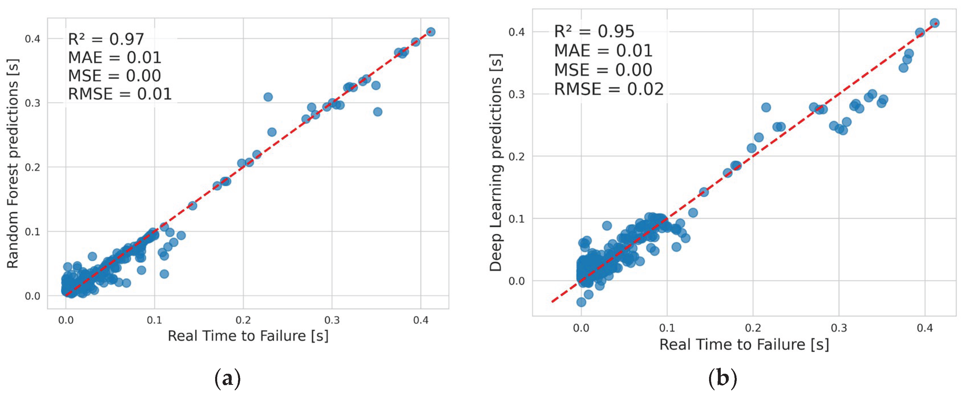
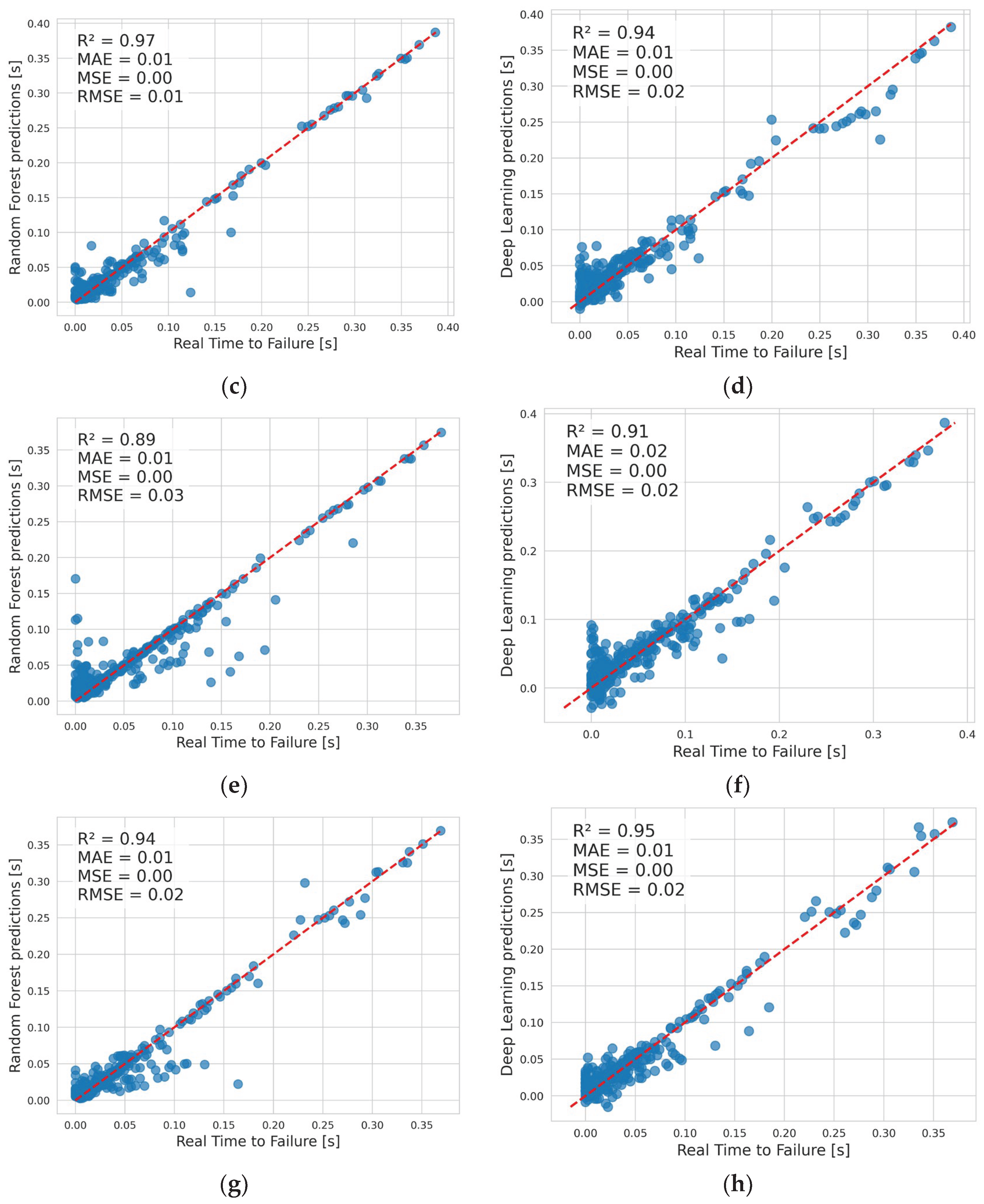
Figure 7.
Computational time for: (a) Experiment 1; (b) Experiment 2; (c) Experiment 3; (d) Experiment 4.
Figure 7.
Computational time for: (a) Experiment 1; (b) Experiment 2; (c) Experiment 3; (d) Experiment 4.
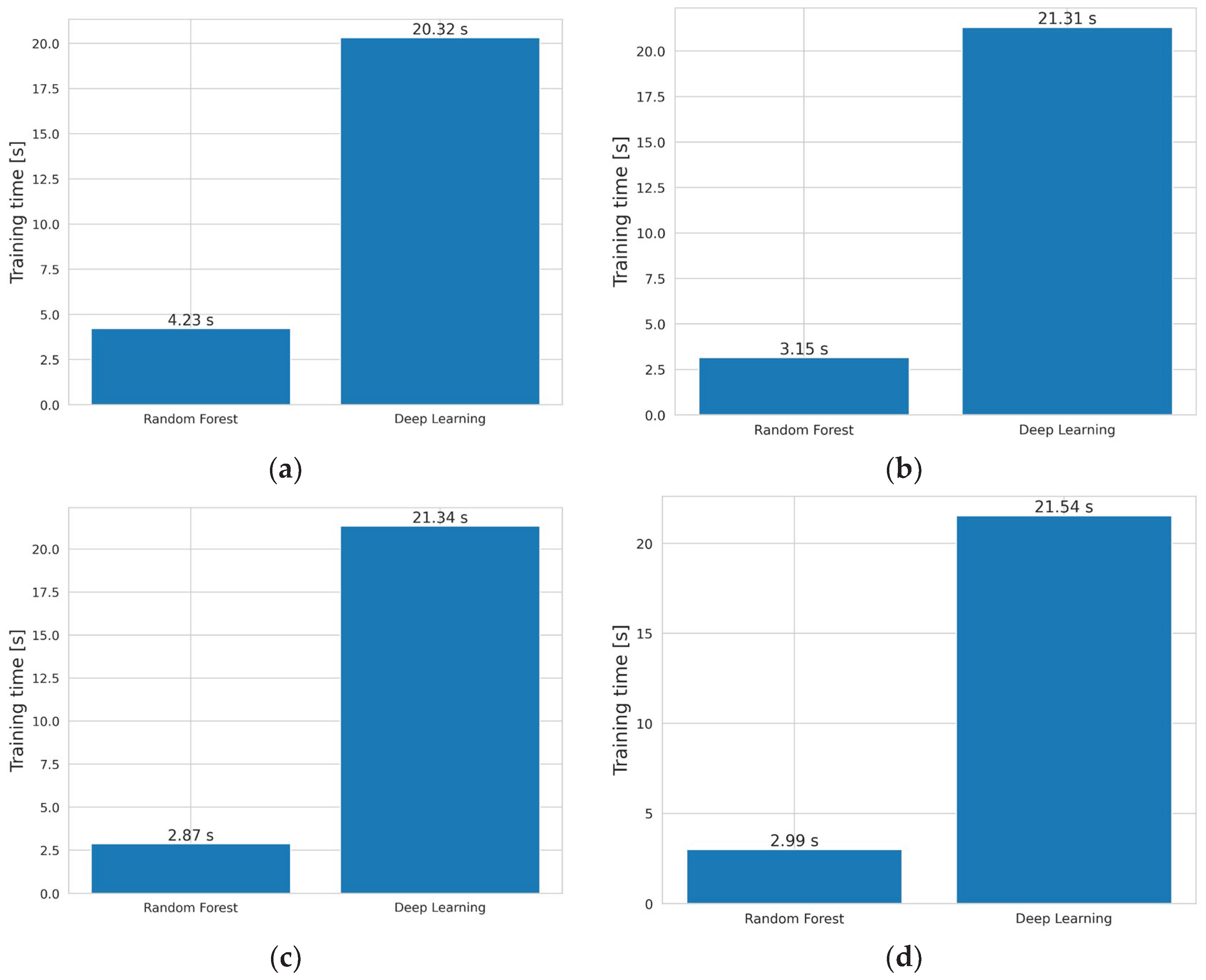
Figure 8.
SHAP values for: (a) Experiment 1 – Random Forest; (b) Experiment 1 – Deep Learning; (c) Experiment 2 – Random Forest; (d) Experiment 2 – Random Forest; (e) Experiment 3 – Random Forest; (f) Experiment 3 – Random Forest; (g) Experiment 4 – Random Forest; (h) Experiment 4 – Random Forest.
Figure 8.
SHAP values for: (a) Experiment 1 – Random Forest; (b) Experiment 1 – Deep Learning; (c) Experiment 2 – Random Forest; (d) Experiment 2 – Random Forest; (e) Experiment 3 – Random Forest; (f) Experiment 3 – Random Forest; (g) Experiment 4 – Random Forest; (h) Experiment 4 – Random Forest.
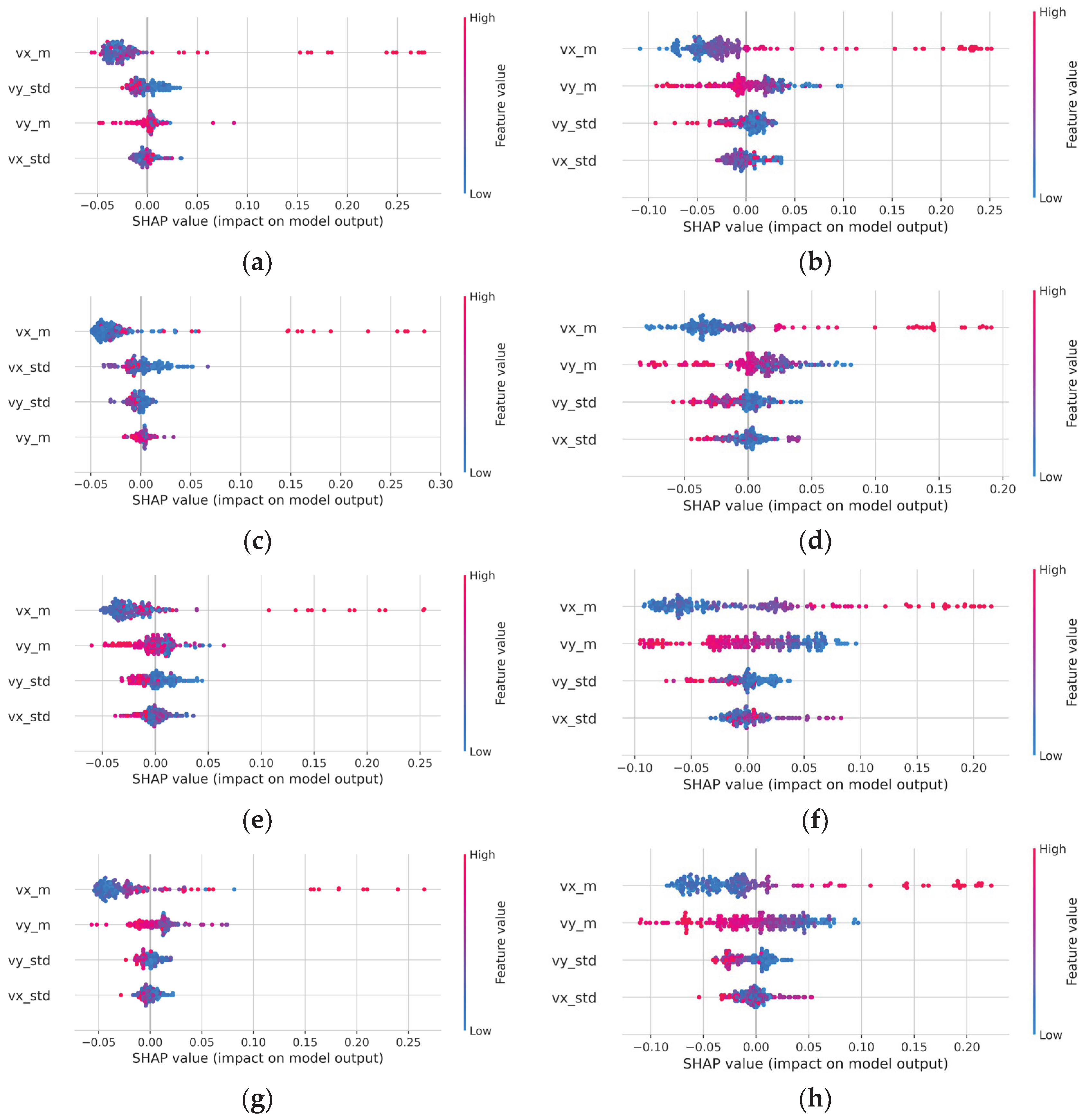
Figure 9.
Visualization of the prediction results for the last 10% of data points (testing dataset) for: (a) Experiment 1; (b) Experiment 2; (c) Experiment 3; (d) Experiment 4.
Figure 9.
Visualization of the prediction results for the last 10% of data points (testing dataset) for: (a) Experiment 1; (b) Experiment 2; (c) Experiment 3; (d) Experiment 4.
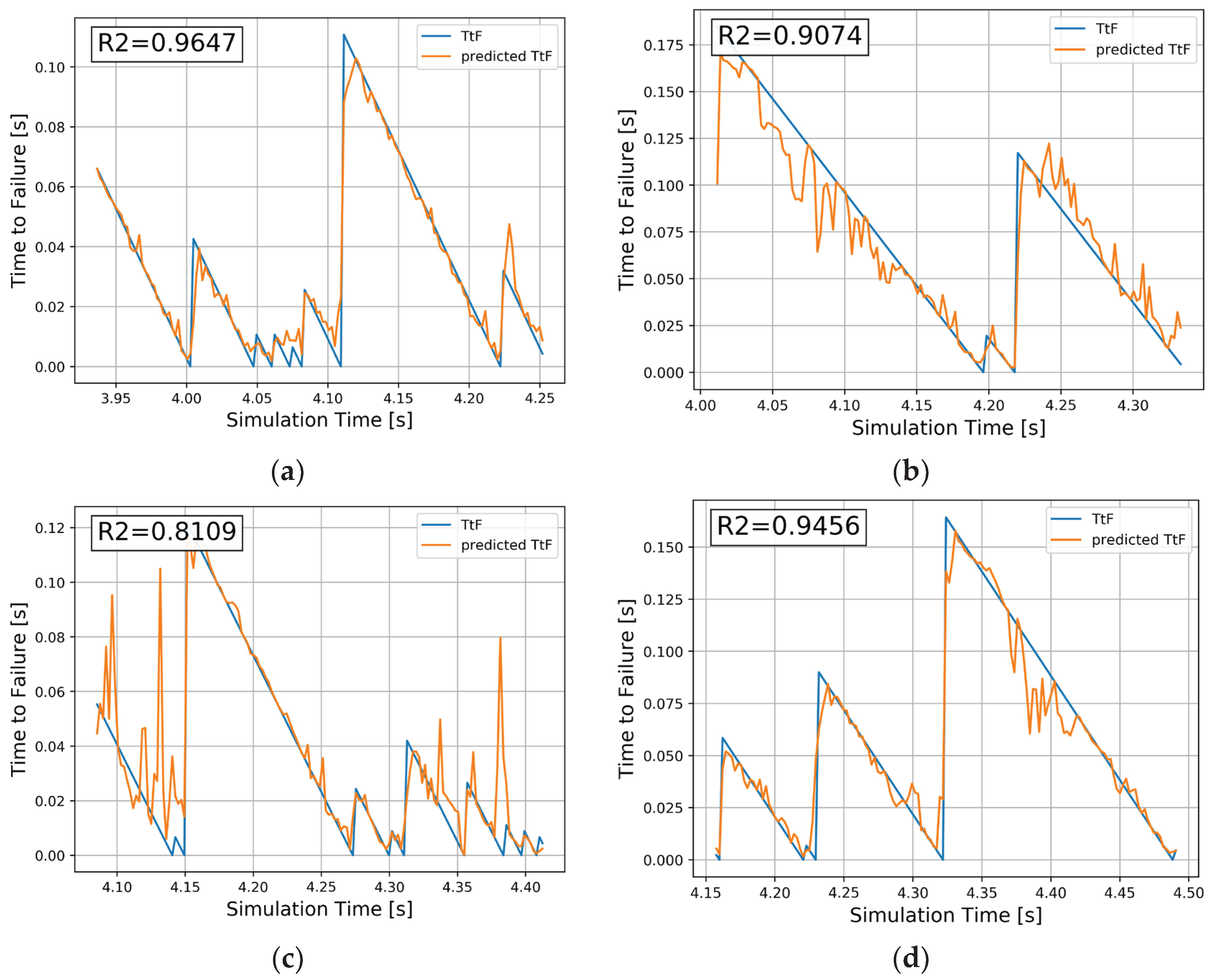

Table 1.
Features used for Time to Failure predictions.
|
Feature1 vx_m |
Feature2 vy_m |
| mean of the X component of the particles’ velocity |
mean of the Y component of the particles’ velocity |
|
Feature3 vx_s |
Feature4 vy_s |
| standard deviation of the X component of the particles’ velocity |
standard deviation of the Y component of the particles’ velocity |
Table 2.
Features used for Time to Failure prediction.
| Experiment | Evaluation metrics | ||||||
|---|---|---|---|---|---|---|---|
| R2 | MAE | MSE | |||||
| RF | DL | RF | DL | RF | DL | ||
|
Training dataset |
E1 | 0.9486 ± 0.0080 | 0.9238 ± 0.0143 | 0.0109 ± 0.0007 | 0.0174 ± 0.0022 | 0.0004 ± 0.0001 | 0.0006 ± 0.0001 |
| E2 | 0.9580 ± 0.0163 | 0.9333 ± 0.0082 | 0.0093 ± 0.00093 | 0.0159 ± 0.0025 | 0.0003 ± 0.0001 | 0.0005 ± 0.0001 | |
| E3 | 0.8906 ± 0.0242 | 0.8608 ± 0.0203 | 0.0137 ± 0.0014 | 0.0204 ± 0.0009 | 0.0007 ± 0.0002 | 0.0009 ± 0.0001 | |
| E4 | 0.9424 ± 0.0177 | 0.9359 ± 0.0105 | 0.0099 ± 0.0009 | 0.0143 ± 0.0013 | 0.0003 ± 0.0001 | 0.0004 ± 0.0001 | |
|
Testing dataset |
E1 | 0.9719 | 0.9434 | 0.0081 | 0.0137 | 0.0002 | 0.0004 |
| E2 | 0.9665 | 0.9572 | 0.0080 | 0.0108 | 0.0002 | 0.0003 | |
| E3 | 0.8858 | 0.8866 | 0.0132 | 0.0196 | 0.0007 | 0.0007 | |
| E4 | 0.9432 | 0.9306 | 0.0094 | 0.0147 | 0.0003 | 0.0004 | |
Disclaimer/Publisher’s Note: The statements, opinions and data contained in all publications are solely those of the individual author(s) and contributor(s) and not of MDPI and/or the editor(s). MDPI and/or the editor(s) disclaim responsibility for any injury to people or property resulting from any ideas, methods, instructions or products referred to in the content. |
© 2025 by the authors. Licensee MDPI, Basel, Switzerland. This article is an open access article distributed under the terms and conditions of the Creative Commons Attribution (CC BY) license (http://creativecommons.org/licenses/by/4.0/).
Copyright: This open access article is published under a Creative Commons CC BY 4.0 license, which permit the free download, distribution, and reuse, provided that the author and preprint are cited in any reuse.


