
Submitted:
11 December 2025
Posted:
12 December 2025
Read the latest preprint version here
Abstract
Classical real analysis rigorously defines convergence via ε − N criteria, yet it frequently regards the specific entry index N as a mere artifact of proof rather than an intrinsic property. This paper fills this quantitative void by developing a radius of convergence framework for the sequence space Seq(R). We define an index-based radius ρa(ε) alongside a rescaled geometric radius ρ∗a (ε); the latter maps the unbounded index domain to a finite interval, establishing a structural analogy with spatial radii familiar in analytic function theory. We systematically analyze these radii within a seven-block partition of the sequence space, linking them to liminf-limsup profiles and establishing their stability under algebraic operations like sums, products, and finite modifications. The framework’s practical power is illustrated through explicit asymptotic inversions for sequences such as Fibonacci ratios, prime number distributions, and factorial growth. By transforming the speed of convergence into a geometric descriptor, this approach bridges the gap between asymptotic limit theory and constructive analysis, offering a unified, fine-grained measure for both convergent and divergent behaviors.
Keywords:
radius of convergence
; real sequences
; liminf–limsup radii
; cauchy radius
; sequence classification
MSC: 40A05(primary); 26A03; 26A15 (secondary)
“When the values successively attributed to the same variable approach indefinitely a fixed value, so as to end up by differing from it by as little as one could wish, this last is called the limit of all the others.”— Augustin–Louis Cauchy (1789–1857)
1. Introduction
1.1. Real-Valued Sequences and Convergence
Real-valued sequences remain one of the most basic but versatile objects in analysis. Classical mathematical literature emphasize the –N definition of convergence, the derived notions of limit inferior and limit superior, and the extension of limits to the extended real line [1]. These tools give a robust qualitative classification of limit behaviour—convergent, divergent to , or oscillatory—and they underpin the standard partition of into convergent and various divergent subclasses [2]. At the same time, the classical framework deliberately abstracts away when a sequence enters a prescribed error band around its limit and focuses instead on the asymptotic fact that such an entry eventually occurs.
Beyond this qualitative viewpoint, several quantitative refinements have been developed. Constructive and computable analysis introduce moduli of convergence or Cauchy moduli, functions that witness how far into the sequence one must go in order to guarantee an -accurate approximation of the limit [3,4,5,6]. Numerical analysis, in turn, describes the speed of convergence of iterative processes via rates and orders of convergence (e.g., “linear,” “superlinear,” or “quadratic” order), capturing how successive errors compare to each other rather than to a fixed -tube [7,8,9]. These perspectives illustrate that quantitative information about convergence is both mathematically rich and practically important.
1.2. Motivation
The present paper is motivated by a parallel line of work on radii of continuity for real-valued functions, where one assigns to each point and tolerance a maximal radius within which the function oscillation around stays below [10]. Such radii encode local stability of functions in the metric space and lead to a fine-grained description of continuity that interacts naturally with algebraic operations and with classical moduli of continuity. From this vantage point, it is natural to ask whether an analogous “radial” description can be developed for sequences in , with the index n playing the role of a one-dimensional “space” variable along the tail of the sequence.
In classical analysis, the phrase “radius of convergence” appears almost exclusively in the context of power series, where one studies the largest spatial radius such that the series converges whenever and diverges whenever [1]. This notion is attached to analytic functions in the complex plane rather than to bare sequences [11]; it is a geometric property of where a series converges, not of how quickly its coefficients or partial sums stabilize. By contrast, the moduli of convergence mentioned above provide index-based information for sequences but are rarely organized or studied through an explicit “radius” vocabulary. Thus, there is a conceptual gap between geometric radii in function spaces and quantitative convergence data in sequence spaces. The goal of this paper is to bridge this gap by introducing and systematically studying radii of convergence for real-valued sequences within the context of constructive mathematical analysis [3,4,5].
1.3. Organization of the Paper
This paper is organized as follows. In Section 2 we provide the necessary mathematical background for the subsequent sections. In Section 3 we introduce the notion of a radius of convergence for sequences, beginning with one-sided liminf and limsup radii and then extending the discussion to the two-sided radius of convergence, the geometric radius, and the Cauchy radius. We then study the stability of these radii under algebraic operations on sequences. Next, in Section 4 we present examples of computing the radius of convergence for two clusters of sequences: four convergent sequences and four divergent sequences with infinite limits. We conclude the paper with a brief discussion in Section 5.
2. Preliminaries
In this subsection we collect the basic notation and standard facts about real-valued sequences that will be used throughout the paper.
Definition 2.1
(Sequence space ). We denote by the space of all real-valued sequences equipped with pointwise addition and scalar multiplication.
Definition 2.2
(Limit inferior, limit superior, limit profile and limit). Let . The limit inferior and limit superior of a are defined by and where in which The pair is referred as limit profile of When , we write and say that a is convergent.
Lemma 2.3
(Tail characterization of lim inf and lim sup). Let , and let be the tail infimum and tail supremum defined by and respectively. Then is increasing, is decreasing, and
In particular, if and only if the monotone sequences and converge to finite real limits.
Definition 2.4
(Cauchy sequence). A sequence is called Cauchy if for every there exists such that
Theorem 2.5
(Cauchy Equivalency Criteria). In the complete space , every Cauchy sequence is convergent, and conversely every convergent sequence is Cauchy.
Theorem 2.6
(Seven-block partition of by lim inf and lim sup). For each let be its limit inferior and limit superior. Define
Then the seven sets are pairwise disjoint and
In particular, every real-valued sequence belongs to exactly one of the blocks , according to the qualitative behaviour of its limit inferior and limit superior (unbounded on both sides, bounded but non-convergent, one-sided unbounded, diverging to or , or convergent) [2].
Lemma 2.7
(Infimum of an intersection). Let be nonempty sets with the following tail property:
Then:
(i)There exist integers such that and
(ii)
Lemma 2.8
(Asymptotic inversion of ). Let be a variable and put . Then, as ,
3. Theory of Radius of Convergence for Sequences
Write a paragraph and tell the readers what you are going to talk about.
3.1. One-Sided Liminf and Limsup Radii for a Single Sequence
We start our investigation by focusing on the limit profile of a given sequence and its associated radii, and their potential relationship:
Definition 3.1
(Liminf and limsup radii). Let be a real sequence with associated tail infimum and tail supremum and let .
(i) We define the liminf radius of a at level by:
(ii) We define the limsup radius of a at level by:
(iii) We refer to the pair as the radii profile of the sequence
Remark 3.2
By the standard properties of lim inf and lim sup, the sets are non-empty for every , hence the corresponding radii are finite integers.
Remark 3.3
As a direct result of Definition 3.1 and Theorem 2.6, there are seven different methods for the computation of radii profile given the limit profile.
Theorem 3.4
(Relations between liminf and limsup radii when the two–sided limit exists). Let be a sequence with associated limit profile and radii profile . Assume Then:
- If , then for every ,
- If , then in general there is no universal inequality between these radii and for given each of the three orderings can occur (see the proof for explicit examples).
- If , then for every ,
Proof.
By Lemma 2.3 the tail infimum and tail supremum satisfy for all N, with increasing and decreasing. We treat the three cases separately.
- (1) Case . Here , and by Definition 3.1 it yields that if , then for all , hence for all , so . Thus and taking infimum from both sides it follows that .
To see that the inequality can be strict, take . Then and , so and . Consequently,
- (2) Case . Then We now show that no universal inequality between and holds in this case, by providing convergent sequences that realize all three orderings for a fixed .
First, define
Then . Every tail contains zeros, so for all N, whence and . On the other hand, , so there exists a least with for all , giving . Thus
Second, define
Again . Every tail contains zeros and negative spikes, so for all N, and hence and . The tail infima satisfy , so there exists a least with for all , and thus . Hence
Finally, for the constant sequence we have for all N, so and . These three examples show that all three orderings between and can occur.
- (3) Case . Here , and by Definition 3.1 it yields that if , then for all , hence for all , so . Thus and taking infimum on both sides, it follows that .
To see that the inequality can be strict, take . Then and , so and , and hence
This completes the proof. □
Conjecture 3.5
(Limit profile vs. Radii profile). Let be a sequence with associated limit profile and radii profile . Then:
Counterexamples. We present two counterexamples each for one direction of implication (11):
(a) :
Let be defined by Then and . Next, for any and we have and Consequently:
(b) :
Let be defined by Then and . On the other hand, for given
Roughly speaking, there is no simple characterization beyond such tail-level regularity.
3.2. Two-Sided Radius of Convergence and Cauchy Radius
We continue our investigation by focusing on the two-sided radius of convergence, the Cauchy (uniform) radius of a given sequence , their potential relationship with each other and to the one-sided radii:
Definition 3.6
(Radius of convergence of a convergent sequence). Let be a convergent real sequence with limit . For we define the radius of convergence of a at level by:
Thus is the smallest index after which the entire tail of a remains within the –tube around its limit L (Figure 1).
Remark 3.7
Given the convergent sequences a, we may view and from Definition 3.1 as one-sided radii relative to the common limit , while in Definition 3.6 is the two-sided radius.
Definition 3.8
(Geometric radius). To emphasize the analogy with classical notions of radius (such as the radius of a ball in a metric space or the radius of convergence of a power series), one may equivalently work with the rescaled radius:
with the convention (Figure 2).
Remark 3.9
The transformation is strictly decreasing on and invertible via
so and encode exactly the same information about the convergence speed of a. In particular, larger values of correspond to smaller entry indices , so that behaves qualitatively like a geometric radius around the limiting point(Figure 2).
Theorem 3.10
(Block-wise two-sided radius of convergence). Let belong to one of the seven blocks of Theorem 2.6, and let be the two-sided radius of convergence of a at level (Definition 3.6). Then is well defined and finite for every if and only if ; for the two-sided radius is not defined, and on the convergent blocks we have that is nonincreasing on G and nondecreasing on .
Proof.
By Definition 3.6 the quantity is defined only when a converges in to a limit , and then
By Definition 2.2 and Theorem 2.6, the sequence a has an extended limit if and only if , i.e. if and only if a lies in one of the convergent blocks ; on the divergent blocks we have , so no extended limit exists and is left undefined there.
If , then and, for ,
whence , so is nonincreasing on G.
If (so ), then for we have
so , i.e. is nondecreasing on E. The case with is analogous, using the sets , and yields the same monotonicity conclusion. Collecting the block-wise information gives Table 1. □
Definition 3.11
(Cauchy radius). Let be a real sequence and . We define the Cauchy radius of a at level by:
Remark 3.12
As the direct result of Definition 3.11 and Theorem 2.5:
Theorem 3.13
(Two–sided radius via liminf / limsup radii). Let and suppose its extended limit exists, i.e. . For let be as in Definitions 3.1 and 3.6. Then:
Proof.
First, we proof the equality (21). We distinguish the cases , , and .
- (a) Finite limit . If , then for every we have for all , hence , so and . Thus . Conversely, if , then for each , so and . Accordingly, .
- (b) Infinite limit . Here, for any n we have iff for all . Hence . Moreover, implies , so .
- (c) Infinite limit . This case is analogous to (b) with all inequalities reversed; again one obtains .
Second, we prove equality (21). In all three cases the sets , , are nonempty tails of . By Lemma 2.7:
This completes the proof. □
Theorem 3.14
(Comparison of two–sided and Cauchy radii). Let be a convergent real sequence with limit , two–sided radius and Cauchy radius . Then, for every and every we have:
Proof.
Fix and , and let . Then for every we have and . If , the triangle inequality gives so . This proves the set inclusion:
Since and are tail sets in , by an application of Lemma 2.7 on inequality (24) we have:
This completes the proof. □
Corollary 3.15
Under the assumptions of the Theorem 3.14, for every we have:
3.3. Stability Under Algebraic Operations
We now collect the main structural properties of the radius of convergence, in terms of its assigned sequence a and other features as follows:
Theorem 3.17
(Stability of the radius of convergence). Let and be convergent real sequences with finite limits and , respectively. Denote by , their radii of convergence in the sense of Definition 3.6. Then the following assertions hold:
- (i)
- Monotonicity and characterization of convergence. For every ,
- (ii)
- Tail invariance under finite modification. If is a sequence with for all for some , then c converges to and
- (iii)
- Affine transformations. Let and , and define . Then and
- (iv)
- Sums. Define and . Then, and
- (v)
-
Products. Define (Hadamard Product) and . For setThen and
- (vi)
- Quotients. Let and be convergent real sequences with finite limits and . Define and Then and, for every ,
Proof. (i) If , then by definition. Now, taking infimum from both sides it follows that .
(ii) If for all and , then clearly . Moreover, by Definition 3.6,
Hence, , and taking infima gives
Since , we conclude
(iii) For and we have
Thus if and only if , and the stated identity for follows by taking infima over N.
(iv) Fix and put for . If , then we have and respectively. Hence
This shows that and therefore , as claimed.
(v) Fix and define as in the statement. Let . Then for every we have
In particular for all , and we may write
Hence, for ,
using in the third line and the definition of in the last line. Thus and the claimed inequality for follows.
(vi) Fix . Since , there exists such that implies . For such n, we can write
Hence a sufficient condition for is that both:
Let and . By Definition 2.13, for all we have , and for all we have . Therefore, for all , inequalities (32) hold and consequently . Hence , and taking infima gives
which proves (31).
This completes the proof. □
Remark 3.18
The inequalities (29)- (31) in Theorem 3.17 can be strict. As examples, it is sufficient to consider the following examples:
For the sum case, take and , so and hence . Solving gives whenever , so for any with we have . Because is constant, for every . Thus for such , so inequality (29) is strict.
For the product case, take and , so and . From we get when , and from we obtain in the same generic case. For (26), with and chosen so that , both radii satisfy and , hence . Since gives , we have for these , so (30) is strict.
4. Examples and Explicit Computations
We present the calculation of radius of convergence for several key classical sequences as follows:
4.1. Radii of Convergence for Classical Convergent Sequences
Example 4.1
(). Let be given by
Then . For we have , and the elementary estimate for yields
The function is strictly decreasing on with . Hence for every sufficiently small there exists a unique real number such that , and for all integers we have . In particular, implying:
Using the expansion as , we have
so solving yields the well-known asymptotic profile
and therefore
Example 4.2
(). Let be given by
It is classical that , hence . For we have
With this yields
Exponentiating and using we obtain
where we used for in the last step. Hence for every and every integer we have for all . In the notation of Definition 3.6, we have implying:
Moreover, from the classical expansion we infer the asymptotic profile
Example 4.3
(Fibonacci ratios ). Let be the Fibonacci numbers and consider
Using Binet’s formula [12]:
we obtain
Since , the ratios converge to and
Taking absolute values and using gives
Thus, for any , every integer
satisfies for all . Consequently
because . Since (42) shows , we obtain the logarithmic asymptotic
Example 4.4
(Leibniz partial sums for ). Define the sequence of partial sums of the Leibniz series by
Then as . Since this is an alternating series with monotonically decreasing terms , the alternating series test yields the sharp remainder bound
and the right-hand side is strictly decreasing in n. Consequently, for we have
Solving the inequality gives , that is,
Therefore the radius of convergence of at level is
and in particular
4.2. Radii of Convergence for Classical Divergent Sequences
Example 4.5
(Geometric progression ). Let be defined by
Then , so in Definition 3.6. Since is strictly increasing, for any the condition
is equivalent to . Hence
Solving for N gives , so the smallest admissible index is
In particular,
where “∼” denotes asymptotic equivalence, not an algebraic equality.
Example 4.6
(The Fibonacci sequence ). Let be the Fibonacci numbers with , and , and define
Then , so . By Binet’s formula,
and since we have for all
Because is strictly increasing, the set is
Example 4.7
(The prime numbers ). Let denote the n-th prime and set
Then , so and
Hence equals the number of primes not exceeding , plus one. Let be the prime counting function. Then
By the prime number theorem (PNT) [13],
and (65) is equivalent to the well–known asymptotic for the n-th prime. Substituting into (65) and using (64) yields
Note that (66) is a consequence of the PNT and its standard asymptotic inversion, not an exact algebraic formula.
Example 4.8
(Factorials ). Let be given by
Then , so and, as in the previous examples,
Thus is the smallest N with . To understand its growth, we use Stirling’s formula
which implies
Set and write heuristically . Taking logarithms and using (69), we obtain
Equation (70) is an asymptotic relation of the form , and its inversion must therefore be understood in the asymptotic sense of Lemma 2.8, not as an exact algebraic division. Applying Lemma 2.8 with and yields
Thus the radius function for the factorial sequence has the standard inverse– growth: it is “almost logarithmic’’ in , with a correction in the denominator. The exact inverse of can be written using the Lambert W–function, but only the leading asymptotics are needed here.
Table 2 presents the summary of radius of convergence of above sequences for the asymptotic cases:
5. Discussion
5.1. Summary of the Radius-of-Convergence Viewpoint in
In this paper we proposed a radius–of–convergence viewpoint for real sequences that complements the classical limit–based description. Starting from the liminf/limsup profile , we introduced the one–sided liminf and limsup radii and , the two–sided radius of convergence , the rescaled geometric radius , and the Cauchy radius . These constructions provide quantitative thresholds for entering an –tube either around the limit interval or around the circular area in , and they remain meaningful for finite and infinite limits alike. We established basic structural properties (monotonicity in , block–wise behavior across the seven–block partition, and stability under algebraic operations such as sums, scalar multiples, and products) and illustrated them on eight representative examples from convergent and –divergent clusters. Altogether, the radii offer a unified language to compare how fast different sequences converge, diverge, or oscillate inside the global space .
5.2. Relation to Classical Cauchy Convergence and Theory
The new radii are tightly linked to standard tools such as Cauchy convergence and the framework. For sequences with , the one–sided radii coincide and the two–sided radius is comparable to the Cauchy radius , so that the finiteness of these radii for every recovers the usual Cauchy criterion. For general sequences, the liminf and limsup radii encode how quickly the tails approach the lower and upper envelope of the limit set, and our comparison results show how is controlled by and , with explicit examples where the corresponding inequalities are sharp or strict. In this way, the radius–of–convergence viewpoint refines the qualitative information carried by lim inf and lim sup into a quantitative scale that still respects the classical Cauchy/limit dichotomy.
5.3. Future Work
The present study suggests several directions for further investigation. First, it would be natural to develop radii for transformed sequences and associated series, for example under linear filters, Cesàro means, discrete differentiation, or when passing from to the partial sums , and to compare these radii with classical notions of convergence acceleration. Second, the interaction between the radii and the seven–block classification, together with the underlying graph structures on blocks, deserves a more systematic analysis; this includes tracking how radii behave along edges of the block graph and identifying “radius–preserving’’ or “radius–contracting’’ transitions between blocks. Third, it would be interesting to extend the framework beyond real sequences, for instance to vector–valued sequences in normed spaces and to random sequences, where one could study Cauchy and convergence radii in almost sure, in–probability, or senses. We hope that these extensions will further clarify how radius–based descriptors fit into the broader landscape of convergence theory.
Funding
This research received no external funding.
Conflicts of Interest
The author declares no conflicts of interest.
References
- Rudin, W. (1976). Principles of mathematical analysis (3rd ed.). New York, NY: McGraw–Hill.
- Soltanifar, M. A classification of elements of sequence space Seq(R). Preprints 2025. [Google Scholar] [CrossRef]
- Bishop, E. Foundations of constructive analysis; McGraw–Hill: New York, NY, 1967. [Google Scholar]
- Bishop, E.; Bridges, D. S. Constructive analysis; Springer–Verlag: Berlin, Germany, 1985. [Google Scholar] [CrossRef]
- Troelstra, A. S., & van Dalen, D. (1988). Constructivism in mathematics: An introduction (Vols. 1–2). Amsterdam, The Netherlands: North-Holland / Elsevier.
- Weihrauch, K. Computable analysis: An introduction; Springer–Verlag: Berlin, Germany, 2000. [Google Scholar]
- Burden, R. L.; Faires, J. D. Numerical analysis, 9th ed.; Brooks/Cole, Cengage Learning: Boston, MA, 2011. [Google Scholar]
- Chasnov, J. R. Numerical methods for engineers [Lecture notes]. Hong Kong, China: Department of Mathematics, Hong Kong University of Science and Technology. 2020. Available online: https://www.math.hkust.edu.hk/~machas/numerical-methods-for-engineers.pdf.
- Rate of convergence. (2014). In Encyclopedia of Mathematics. European Mathematical Society. Retrieved from http://encyclopediaofmath.org/wiki/Rate_of_convergence.
- Soltanifar, M. An atlas of epsilon-delta continuity proofs in function space F(R, R). Preprints 2025. [Google Scholar] [CrossRef]
- Ahlfors, L. V. Complex analysis: An introduction to the theory of analytic functions of one complex variable, 3rd ed.; McGraw–Hill: New York, NY, 1979. [Google Scholar]
- Knuth, D. E. (1997). The art of computer programming: Vol. 1. Fundamental algorithms (3rd ed.). Reading, MA: Addison–Wesley.
- Ingham, A. E. The distribution of prime numbers; (Original work published 1932); Cambridge University Press: Cambridge, UK, 1990. [Google Scholar]
Figure 1.
Radius of convergence for a convergent sequence . The shaded horizontal strip is the -band around the limit . The earliest admissible index is ; for the tail still leaves the band (inadmissible), while for the tail from each such index onward is contained in the band.
Figure 1.
Radius of convergence for a convergent sequence . The shaded horizontal strip is the -band around the limit . The earliest admissible index is ; for the tail still leaves the band (inadmissible), while for the tail from each such index onward is contained in the band.
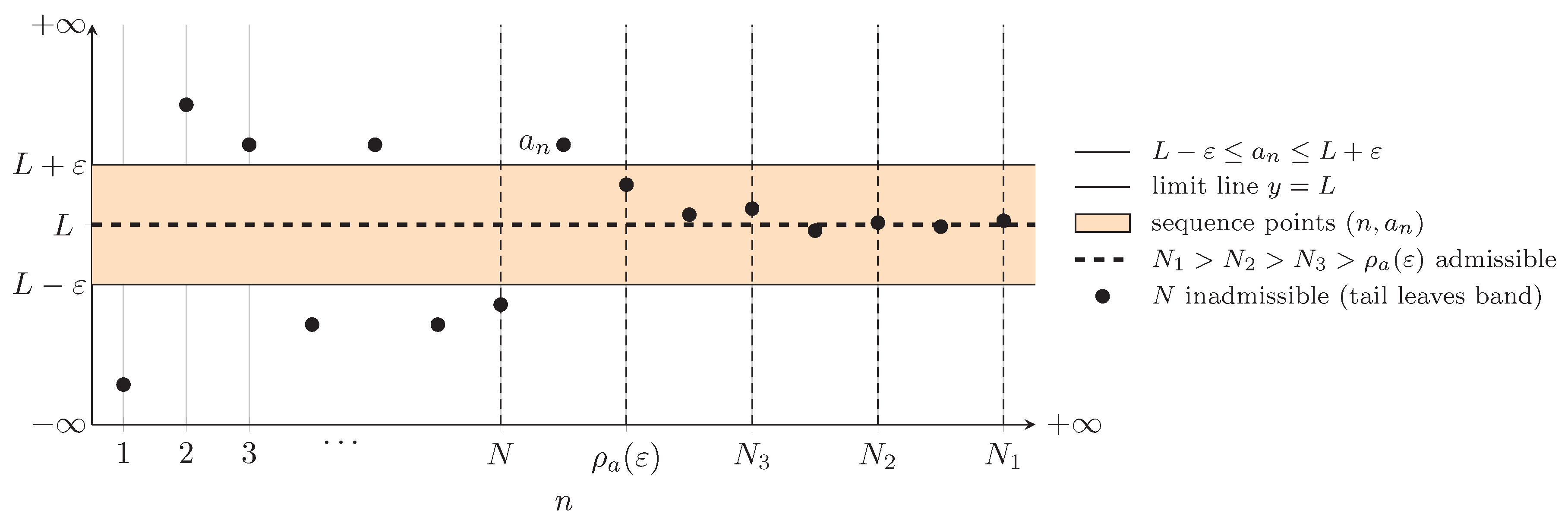
Figure 2.
Geometric representation of the rescaled radius of convergence. The white reference disk A has centre and radius (dashed boundary). For a fixed , the geometric radius determines the inner disk (orange region), with whenever . In this schematic we take for clarity: the early terms and the closest outsider (squares) lie in the annulus , while the tail terms and the remaining spiral points (dots) converge to the starred limit point inside the orange disk.
Figure 2.
Geometric representation of the rescaled radius of convergence. The white reference disk A has centre and radius (dashed boundary). For a fixed , the geometric radius determines the inner disk (orange region), with whenever . In this schematic we take for clarity: the early terms and the closest outsider (squares) lie in the annulus , while the tail terms and the remaining spiral points (dots) converge to the starred limit point inside the orange disk.


Table 1.
Block-wise behaviour of the two-sided radius of convergence .
| Block | Limit profile | Radius profile of |
| A | not defined (no extended limit) | |
| B | not defined (no extended limit) | |
| C | not defined (no extended limit) | |
| D | not defined (no extended limit) | |
| E | for all ; nondecreasing in | |
| F | for all ; nondecreasing in | |
| G | for all ; nonincreasing in |
Table 2.
Convergence and geometric radii for the classical sequences of Section 4(all relations are asymptotic).
Table 2.
Convergence and geometric radii for the classical sequences of Section 4(all relations are asymptotic).
| # | Name of Sequence | Convergence radius | Geometric radius |
| 1 | |||
| 2 | |||
| 3 | Fibonacci ratios | ||
| 4 | Leibniz partial sums for | ||
| 5 | Geometric progression | ||
| 6 | Fibonacci numbers | ||
| 7 | Prime numbers | ||
| 8 | Factorials |
Disclaimer/Publisher’s Note: The statements, opinions and data contained in all publications are solely those of the individual author(s) and contributor(s) and not of MDPI and/or the editor(s). MDPI and/or the editor(s) disclaim responsibility for any injury to people or property resulting from any ideas, methods, instructions or products referred to in the content. |
© 2025 by the authors. Licensee MDPI, Basel, Switzerland. This article is an open access article distributed under the terms and conditions of the Creative Commons Attribution (CC BY) license (http://creativecommons.org/licenses/by/4.0/).
Copyright: This open access article is published under a Creative Commons CC BY 4.0 license, which permit the free download, distribution, and reuse, provided that the author and preprint are cited in any reuse.


