Submitted:
11 December 2025
Posted:
14 December 2025
You are already at the latest version
Abstract
This article investigates the trajectory-tracking control of a differential-drive two-wheeled mobile robot (DDWMR) using its kinematic model. A nonlinear-to-linear transformation based on differential flatness is employed to convert the original nonlinear system into two fully decoupled linear subsystems, enabling a simple and robust controller design. Unlike conventional flatness-based methods that rely on exact feedforward linearization around a reference trajectory, the proposed approach performs plant linearization, ensuring reliable tracking across a wide range of trajectories. The resulting two-loop architecture consists of an inner nonlinear loop implementing state prolongation and static feedback, and an outer linear controller performing trajectory tracking of the linearized system. Simulation results on a circular reference trajectory demonstrate high tracking accuracy, with a maximum transient deviation of 0.28 m, a settling time of approximately 120 s, and a steady-state mean tracking error below 0.01 m. These results confirm that the plant-linearization-based framework provides superior accuracy, robustness, and practical applicability for DDWMR trajectory tracking.
Keywords:
wheeled mobile robot (WMR)
; nonlinear control
; trajectory tracking
; differential flatness
; computed torque control (CTC)
; smart mobility programming
1. Introduction
Mobile robot control has been an active research topic over the past three decades due to its wide range of practical applications, including mineral resource development, logistics and transportation, planetary exploration, agriculture, and defense, among others [1,2,3,4]. Beyond core algorithms and hardware, contemporary mobile robotics is increasingly shaped by sustainability and Environmental, Social, and Governance (ESG) requirements at the application level. IEEE 7000:2022 provides process-oriented guidance for value-based, ethically aligned engineering across the entire product lifecycle—from stakeholder value elicitation through design requirements, verification, and field operation of robotic systems [5]. In particular, the IEEE 7007:2021 provided and ontology based framework to support the responsible and sustianable development of autonomous systems [6]. The contribution of mobile robots has also been mapped to the United Nations Sustainable Development Goals (SDGs): improving the efficiency and safety of work, logistics, and manufacturing (SDGs 8, 9, 11); energy-efficient motion planning and resource-aware operation (battery usage, wear, maintenance) (SDGs 7, 12, 13); environmental and industrial safety monitoring (SDGs 3, 6, 13); and inclusive human–robot interaction and service accessibility (SDGs 10, 11) [7]. In this study, these considerations are incorporated explicitly: the chosen speed-and-heading control scheme enables sustainability metrics (cycle energy expenditure, braking/acceleration intensity, predicted actuator wear) to be embedded in the objective functions and controller constraints, while preserving requirements’ traceability—from value and risk levels to reference-signal filters and compensation channels. This strengthens the rationale for the selected compensation algorithms and multi-channel control aimed at improving the reliability and safety of WMR operation.
A distinctive feature of many mobile robotic systems is the presence of non-integrable (i.e., nonholonomic) kinematic constraints [8]. This, by itself, substantially complicates control synthesis; moreover, for nonholonomic mobile robots the necessary condition for smooth stabilization (Brockett’s condition) is often not satisfied [9], which makes trajectory-tracking and path-following particularly challenging. In recent years, a wide range of methods has been proposed and applied to nonholonomic mobile robots, including sliding-mode control [10,11,12], backstepping [13], and nonlinear model predictive control (NMPC), as well as feedback-linearization and Lyapunov-based designs.
1.1. Differential-Flatness–Based Trajectory Control
Among trajectory-tracking methods for nonlinear control systems, differential-flatness–based approaches play a particularly important role. If the controlled plant is differentially flat, the trajectory-tracking problem can be feed-back-linearized—that is, a difficult nonlinear design reduces to a comparatively simple and well-studied linear control problem. Historically, flatness theory emerged from trajectory planning and tracking; interest in flatness-based control persists because flat systems possess properties that make trajectory generation and implementation especially effective.
Not every control system is flat. A flat system is characterized by the existence of a flat (linearizing) output such that, at any instant, the full state vector and the control inputs are algebraic functions of this output and a finite number of its time derivatives. Intuitively, by observing only the flat output one can reconstruct the state and the input without direct measurement. The corresponding mappings act as an inverse model of the nonlinear plant, which explains the affinity between flatness-based controllers and inverse-model designs; more generally, flat systems are dynamically equivalent to a trivial controllable linear system (e.g., Brunovský form). In practice, flatness is established constructively by exhibiting a suitable flat output as a function of the state, the input, and finitely many input derivatives.
For wheeled mobile robots, several classes are known to be differentially flat under no-slip assumptions [14], or under appropriate inertia distributions for certain underactuated mobile manipulators [15]. In the differential-drive case, a common choice of flat output is the time trajectory of the midpoint of the axle connecting the drive wheels.
1.2. Differential-Flatness–Based Trajectory Control for Wheeled Mobile Robots
A number of differential-flatness–based trajectory-tracking methods have been proposed and experimentally validated for differential-drive wheeled mobile robots [16,17]. These methods share a common controller-design paradigm known as exact feedforward linearization. The approach, introduced by Hagenmeyer and Delaleau [18], rests on the following idea: for a flat system, there exists a mapping that reconstructs the current control input from the flat output and a finite number of its time derivatives. In practice, this mapping can be viewed as a physically realizable operator acting on the flat-output signal. In case the desired trajectory of the flat output is applied to the input of this operator, its output generates a control signal that under suitable regularity and invertibility conditions, drives the plant to follow the prescribed trajectory.
Importantly, even in the absence of disturbances, the resulting motion is determined by both the control signal and the initial state. When the plant’s initial condition exactly matches that implied by the desired flat-output trajectory, the plant’s flat output coincides with the reference. In realistic settings, initial conditions are only known within some tolerance; consequently, exact feedforward linearization requires the initial state to lie within a neighborhood of the nominal initial condition associated with the designed reference trajectory.
The described feedforward trajectory controller can only maintain the plant’s state locally in the vicinity of the desired trajectory. In the absence of a feedback loop, even arbitrarily small deviations caused by mismatch between the actual initial state and the reference, or by external disturbances—tend to grow over time, eventually reaching unacceptable levels; in other words, a purely feedforward scheme is unstable. Consequently, the feedforward path is complemented with a linear feedback structure (e.g., PD/PI/PID acting on tracking errors) to stabilize the closed loop and provide robustness around the reference trajectory.
Despite its inherent limitations, this flatness-based trajectory-tracking approach remains popular and often dominant in mobile robotics because it offers several practical advantages. Notably, an open-loop linearizing feedforward input can render the closed-loop behavior equivalent (locally) to a linear system in Brunovský canonical form, thereby reducing control of a nonlinear plant potentially with nonholonomic constraints to a standard linear design problem. In practice, feedforward linearization yields effective local regulation and tracking across a broad class of nonlinear plants; controllers devised in this framework typically maintain good performance even for intricate reference paths [17].
At the same time, exact feedforward linearization is only one member of the flatness-based toolkit, relying on a specific approximate linearization along the reference. In theory, any differentially flat system admits (coordinate) transformation and dynamic state feedback that convert it into an equivalent linear controllable system [19]; conversely, any nonlinear system that is dynamically feedback-linearizable is flat [20]. Trajectory-tracking architectures built on such (global) dynamic feedback linearization differ fundamentally from exact feedforward linearization: the linearized plant remains linear regardless of the current state, so these controllers do not rely on the actual trajectory staying arbitrarily close to the reference at all times, avoiding the principal drawback of the pure feedforward design.
The differences between exact feedforward linearization and linearization methods that convert a nonlinear flat plant into an equivalent linear controllable system stem from distinct underlying concepts. The “flat-output” viewpoint defining flat systems via the existence of a flat (linearizing) output—naturally aligns with exact feed-forward linearization, which reconstructs the input from the reference flat output and its finite derivatives. By contrast, the system-equivalence viewpoint central to flatness theory underpins dynamic feedback linearization, wherein a suitable change of coordinates combined with dynamic state feedback renders the plant equivalent to a linear system [19]. In fact, within this framework, the existence and properties of a flat output follow as consequences of equivalence to a trivial linear system; thus, defining flatness primarily via a flat output can be seen, theoretically, as Inverting cause and effect [20].
From a practical perspective, the equivalence-based theory of flat systems characterizes a class of transformations between control systems whose associated mathematical operations correspond to physically realizable signal processors. This perspective provides a constructive toolbox for building implementable linearizing controllers, beyond the locality inherent in exact feedforward designs.
Strikingly, although flatness theory for control systems crystallized in the 1990s (e.g., Fliess and co-authors; see the foundational work on the geometric notion of system equivalence [21]), practical trajectory-tracking methods for nonlinear flat systems predate these theoretical developments. A prominent example is CTC, also known as inverse-dynamics control, originally developed for serial robotic manipulators. As shown later in this paper, CTC realizes a static-feedback linearization that maps a non-linear plant into a trivial linear controllable form (Brunovský canonical form), thereby enabling standard linear tracking design with excellent performance and comparatively simple implementation. Notably, nonlinear flat systems such as the kinematic and dynamic models of a differential-drive wheeled mobile robot share an important structural feature with serial manipulators: the flat output coincides with a component of the state vector, which makes the linearizing construction particularly transparent.
Sun et al. conducted a comparative study of one of the most widely used mobile-robot control techniques—Model Predictive Control (MPC)—and differential-flatness-based control for quadrotor agile flight, demonstrating that flatness-based methods provide superior tracking performance [18,22]. Ongoing research continues to explore various differential-flatness-based control techniques, including MPC-based approaches [15,16], optimal control formulations [23], and hybrid combinations of multiple techniques [24,25].
The trajectory-tracking method proposed in this paper is closely related to CTC. The linearization procedure employed herein is conceptually analogous to static-feedback linearization used in MPC and in modern robust and adaptive control frameworks for manipulators and manipulator-like systems [26,27,28]. The authors have previously applied inversion-based modelling techniques [29], as well as trajectory tracking based on endogenous linearization of the dynamic differential-drive WMR model [30], and differential–geometric methods for manipulator control [31,32,33]. Building on these results, the authors aim to generalize the CTC trajectory-control scheme so that it can be applied to differentially flat systems such as wheeled mobile robots, while preserving its simplicity and high-performance properties.
The goal of this study is to linearize the kinematic model of a DDWMR, where linearization is understood as a physically realizable transformation of the nonlinear plant into an equivalent linear controllable system (i.e., a trivial linear system), rather than an approximate linearization in a neighborhood of a reference trajectory, as in exact feedforward linearization. Of particular interest is assessing whether the CTC-inspired linearization enables DDWMR motion to be controlled analogously to the motion of a point in the plane, which, in principle, allows achieving the maximal theoretically attainable trajectory-tracking accuracy.
1.3. Relevance to Sustainable Development Goal 11 (Sustainable Cities and Communities)
Smart and sustainable urban mobility refers to “a modern approach to urban transport that aims to improve the flow of people and goods, reduce congestion and environmental impact, while increasing efficiency, accessibility, and user convenience” (https://www.sciencedirect.com/topics/social-sciences/smart-urban-mobility). It builds on advanced communication systems [36] and transparent and highly customizable control solution for the mobile robots within the smart city ecosystem. Regarding the latter, the proposed linearization and trajectory-control framework contributes to SDG 11 by advancing autonomous mobile robotic systems that can support safer, more efficient, and more sustainable urban environments. Differential-drive WMRs equipped with energy-aware control architectures are suitable for logistics, inspection, mobility, and monitoring tasks in smart-city infrastructures. By improving motion reliability, resource efficiency, and operational safety, the presented method aligns with the development of resilient, technology-integrated, and sustainable cities. Similar approaches have been developed for smart usrban aerial mobility systems [37].
2. Problem Statement
2.1. Hardware-Implementable Transformations of Control Systems and System Equivalence
The trajectory-tracking method proposed in this work for a differential-drive wheeled mobile robot is based on a hardware-implementable transformation of the robot’s kinematic model that converts it into an equivalent trivial linear control system. To clarify the precise meaning of the terminology used, let us consider a simple example of a hardware-implementable transformation of a control system into an equivalent control system . Let be a control system with state space , control space , and dynamics given by (1), and let be a control system with state space , control space and dynamics given by (2).
Let the state spaces of systems and equivalent to each other in the geometric sense of the term; that is, suppose there exists a continuous, invertible mapping , that establishes a one-to-one correspondence between the points of the state spaces and . The control spaces and of these systems are likewise assumed to be mutually equivalent. Consider now the scheme of a hardware-implementable transformation of system B, shown in Figure 1. The block with inputs and is a signal processor that physically implements a prescribed algebraic mapping , while the block represents the hardware implementation of the inverse mapping .
Under certain conditions (see Note 1) imposed on the mappings and , which define the hardware-implementable transformation, as well as on the functions and , that specify the dynamics of control systems and , the block diagram inside the “black box” with input and output becomes equivalent (in the usual practical sense of the term) to control system . More precisely, if the initial state of control system related to the initial state by the relation , to to the system input defined on the time interval , is applied to the input of system and to the input of the transformed system B, then the state trajectories of the outputs of these systems, denoted in Figure 1 by , will coincide at any moment of time . Thus, the object inside the “black box” behaves exactly as the control object described by the mathematical model of system , and we may say that such a hardware-implementable transformation converts control system into control system . Throughout the remainder of this work, when referring to the equivalence of control systems, we shall mean a precisely defined mathematical concept associated with the sets of trajectories of control systems. Recall that a trajectory of a control system defined by the state space , the control space and the dynamical Equation (1), is an application , whose components satisfy the system’s dynamical equation.
To denote trajectories of control systems and their components, we will use the notation , implying that the components of the mapping and , called respectively the state trajectory and the control-input trajectory, satisfy condition (3), where is a finite or infinite time interval.
One may observe that when referring to the equivalence of two control systems, we are in fact speaking about the equivalence of the corresponding sets of trajectories generated by these systems.
Note 1. Under Conditions 1 and 2, the control systems and introduced in the example at the beginning of this section are equivalent.
Condition 1. For any point the mapping defined by formula (4), is a diffeomorphism. This requirement ensures the existence of a smooth, bijective correspondence between the admissible control inputs of the two systems.
Condition 2. For the functions and and for the mappings under consideration, relation (5) holds.
When these conditions are satisfied, the trajectories of control systems and are related by the diffeomorphic mapping , defined by expression (6).
Moreover, is an arbitrary trajectory of system and is the corresponding trajectory of system , then for any moment of time the equalities given in and (see Figure 2).
There exist several different approaches defining the notion of equivalence between control systems. In this article, we adopt the geometric approach first introduced in [21], which is based on analogies between control systems and continuous dynamical systems. Both control systems and continuous dynamical systems can be viewed as geometric objects of the same type—so-called systems. A system is defined as a pair , where – is a smooth manifold and is a tangent vector field on . It is worth noting that the dynamical equation of system (1) corresponds to the infinite system of differential equations given in (7).
where and . Thus, may be regarded as a tangent vector field defined on the infinite-dimensional manifold associated with ., and the control system under consideration may be viewed as the infinite-dimensional dynamical system corresponding to . In [21], an approach was first introduced in which control systems are defined as infinite-dimensional systems , equipped with a Fréchet topology, and a definition was given for an endogenous transformation that relates equivalent control systems represented as such infinite-dimensional systems. Naturally, from a practical standpoint, the cases of greatest interest are those in which a nonlinear control system is equivalent to a linear one. A control system that is equivalent to a so-called trivial linear control system (the definition of this class of linear systems is given below) is referred to as a flat control system.
Definition 1. A linear control system with control space and state space , whose state vector is of the form , and whose dynamics are given by (8), where is called a trivial linear control system.
We denote a trivial linear control system by , where the integer index represents the dimension of the control space, and the index denotes the number of components of the trivial linear system . In this article, we propose a linearisation procedure for the kinematic model of a differential-drive wheeled mobile robot, by which the robot’s kinematic model is transformed into the trivial control system . The linear control system admits a physical interpretation as the dynamics of a material point moving in the plane under the action of a planar force vector. Thus, the linearisation method described in this work reduces the control problem for a highly nonlinear plant to a simple linear control problem with an efficient solution. The proposed linearisation approach is carried out in two stages, which are presented in Section 3 and Section 4. Section 5 provides a description of the trajectory-tracking control system for the linearised kinematic model of the DDWMR.
2.2. Kinematic Model of a Differential-Drive Wheeled Mobile Robot and Class I Transformations
Consider the kinematic model of a differential-drive wheeled mobile robot moving on a horizontal plane. As state variables fully describing the robot’s position and orientation, it is convenient to choose the coordinates of point in a fixed “world” Cartesian coordinate frame together with the robot’s heading angle (see Figure 3). Let denote the velocity vector of point and let and denote the velocity vectors of the centers of the left wheel (point ) and the right wheel (point ), respectively.
We may regard points and as the endpoints of a rigid, thin rod (the imaginary “rear axle” of the robot), whose midpoint is point . All three points therefore belong to the same rigid body—the robot chassis. As is well known [34,35], for the velocity vectors and of any two points and of a rigid body, the relation given in (9) holds, where is the angular velocity vector of the body.
The robot’s angular velocity vector Ω is perpendicular to the floor plane. Accordingly, if we denote by the unit vector normal to the plane, then the angular velocity vector may be written as . In what follows, when referring to the angular velocity of the robot, we shall mean the scalar quantity , whose sign determines the direction of rotation of the robot’s chassis in the horizontal plane. In the absence of lateral slip of the drive wheels, the vectors and are perpendicular to the axle . As follows from Equation (9), applied to points and , the projections of and onto the axis satisfy equality (10) at any moment of time.
Using Equation (10), it is straightforward to show that the vector is parallel to the vectors and . Consequently, the velocity of point can be written as , where is the unit vector aligned with the robot’s heading direction. Furthermore, from the general relation (9) applied to points and equality (11) follows.
Equations (10) and (11) together imply Equations (12).
The above statement regarding the direction of the vector together with the fact that the time derivative of the heading angle, is precisely the angular velocity of the robot’s chassis, leads to the system of differential Equations (13).
Equations (13) can be regarded as the dynamical equations of a control system with state space and control space , representing the simplest kinematic model of a differential-drive wheeled mobile robot. The state vector of this model, , describing the robot’s position and orientation on the plane, is given by , and the control vector is . In what follows, we refer to the above-defined control system as kinematic model. This simplest DDWMR model is convenient for analytical manipulations; however, for computer simulations we employed a more detailed and realistic kinematic model, denoted as model , which is described below. In the absence of longitudinal slip, the velocities of the wheel centers and satisfy relations (14), where is the radius of the robot’s wheels, and and are the angular velocities of the right and left drive wheels, respectively (with and denoting the wheel shaft rotation angles, which may be measured using incremental rotary encoders).
Taking Formulas (14) and (12) into account, system (13) can be rewritten in the form given by (15).
We may regard system (15) as the representation of the coordinate-wise projections of the general dynamical equation of a control system for the state vector . The kinematic model of the robot, denoted as model is transformed into the “advanced’’ robot model by means of the control-signal transformation specified by formulas (16).
The general scheme of the transformation from system A to system B is shown in Figure 4.
We transform the kinematic robot model A into a control system with state space , where and control space whose state vector has the form , and whose dynamics are given by (17).
System Q is obtained by transforming the control signal of the robot’s kinematic model (where are aliases for ) into the control signal of system Q (where are aliases for ), analytically defined by equations (18).
This transformation is an example of a Class control-system transformation, the definition of which is given below. Recall that a control system , is equivalent to the system , , since both systems are described by the same infinite-dimensional system , where the tangent vector field is defined by . Let the control signal of a control system be -dimensional and written as, and let be a linear operator whose action on the signal is defined by equation (19).
It is evident that the control system , is equivalent to the original control system , . We shall refer to such transformations of control systems as Class transformations.
Figure 5.
Hardware-implementable scheme for transforming the DDWMR kinematic model A into the control system
Figure 5.
Hardware-implementable scheme for transforming the DDWMR kinematic model A into the control system
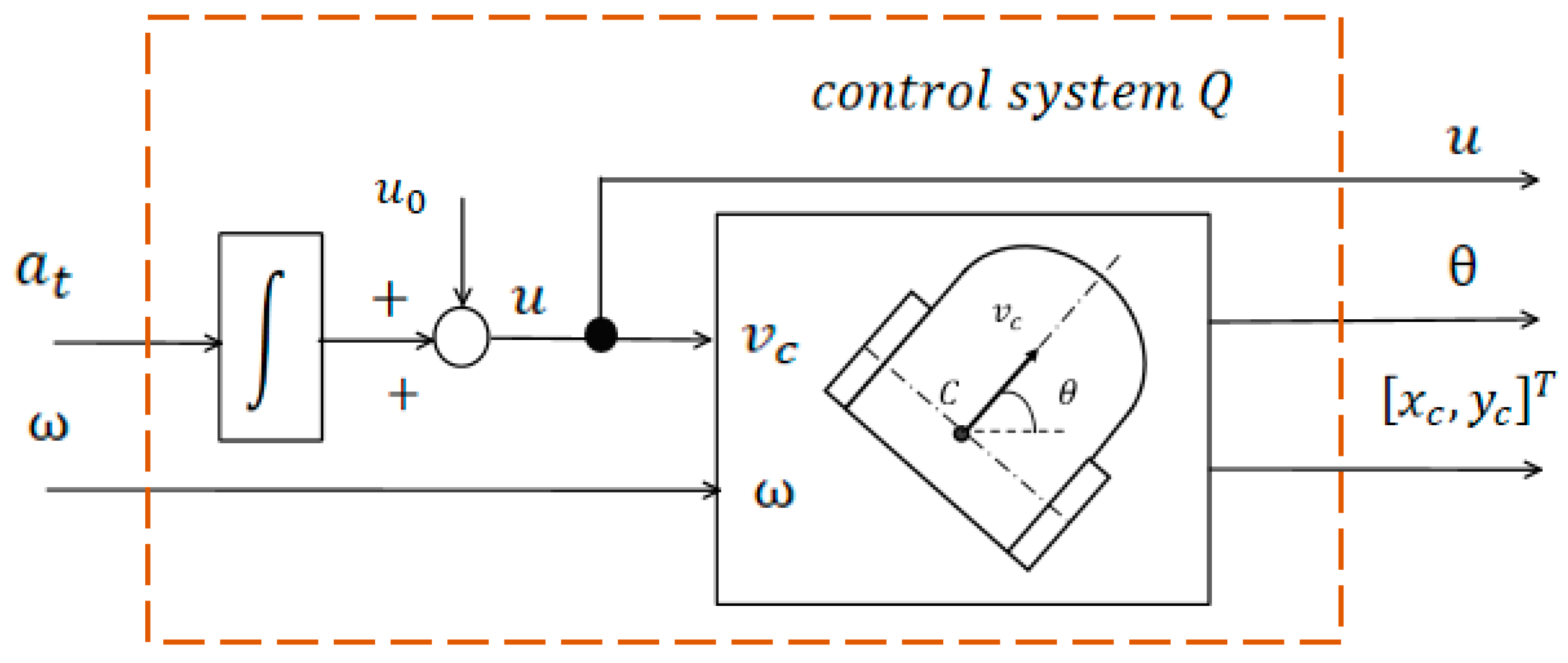
As will be shown in the next section, the control system can be interpreted as a kinematic control system governing the motion of a point in the plane. Accordingly, if we construct a physically implementable transformation that maps this system into the trivial control system , which describes force-based control of a material point moving in the plane, then we will be able to control the motion of the wheeled mobile robot in the same manner as controlling the motion of a point in the plane.
2.3. Linearisation of the DDWMR Kinematic Model
The problem of linearising the control system , defined in the previous section, reduces—as will be shown below—to the linearisation of a simple control system on the smooth manifold . Interestingly, the solution to this problem, presented below, leads directly to a hardware-implementable scheme for linearising the kinematic model of the wheeled mobile robot. First, observe that the kinematic equation , which describes the motion of a point in the plane, may be viewed as the dynamical equation of the trivial linear control system with state space and control space . We assume that the linear space is equipped with an orthonormal basis , б whose basis vectors correspond to the coordinate axes of the Cartesian frame in which the point moves. Any nonzero vector can be represented in the form (20).
where , and the mapping is defined for any by , with being the angle between the vector and . Clearly, for any nonzero vector there exist two possible representations of this form, given by expressions (21) and (22).
Formulas (21) and (22) can be viewed as two coordinate representations of mappings from the Euclidean plane onto the smooth manifold , which we denote by and . For the coordinates of a vector expressed in the form un(θ), the identities (4) clearly hold. These identities may be interpreted as defining the mapping, which serves as the inverse (on their respective domains of definition) to the mappings and
Note that the embedding of the smooth manifold into the three-dimensional Euclidean space is represented by the lateral surface of an infinite cylinder, on which one can introduce coordinates , as illustrated in Figure 6. By expressing vectors of the Euclidean plane in the form (20), we effectively identify each nonzero vector with a point on the surface of this infinite cylinder. Consequently, any state trajectory of system (with the exception of the degenerate trajectory of a stationary point) corresponds to two curves μ+ (γ) and μ- (γ) on the cylinder surface. Let us define a control system with state space , control space , and dynamics As will be shown below, the geometric relationship between trajectories in the phase spaces and , determines a correspondence between the trajectories of systems and as a whole, thereby inducing a transformation from system to system . This transformation is precisely what we refer to as the linearisation of system . Since system constructed on top of system the physically realisable hardware scheme that linearises system simultaneously linearises system . The smooth manifold is not homeomorphic to the plane , in particular, the cylinder cannot be continuously deformed into the Euclidean plane. For this reason alone, there cannot exist a one-to-one correspondence between the full trajectory sets of systems and . However, under the kinematic interpretation of system it becomes clear that not all trajectories of system are physically realisable. Therefore, it is meaningful to speak of an equivalence between the trajectory set of system and the set of physically realisable trajectories of system . To analyse the geometric relationship between the spaces and , we use the identification of vectors of with points on the plane endowed with the Cartesian frame . Define the region by the condition The mapping may then be visualised as the projection of an infinite cylindrical surface, cut by the plane , perpendicular to the cylinder axis , as shown in Figure 7. Each of the regions and , corresponding respectively to the upper and lower halves of the cylinder, is mapped onto the plane with the origin with coordinates removed. The intersection of the cylinder with the plane, which forms a one-dimensional manifold homeomorphic to , is mapped to the single point .
Thus, mapping ends each point of the manifold to a corresponding point on the Euclidean plane . Let denote the subset of the plane that is the image of regions and under mapping . Then the mappings and are defined by equations (1) and (2) respectively. Mapping is a diffeomorphism, and , as denotes the restriction of the mapping to the region . Similarly, the mappings and define a diffeomorphism between the regions and . Let be a parametrically defined curve on the plane , that does not pass through the point . Let us denote the image of the curve under the diffeomorphism , this image is a parametrically defined curve on the manifold given by relation . Likewise, let, and as denote the image of the curve under the mapping . The images of the curves under the mapping π are curves on the plane Х. Moreover, these curves are related by a symmetry transformation defined by an automorphism , introduced below. Specifically, for every the following relations , and hold (see Figure 7). The automorphism is defined by formulas (24), which specify the correspondence between the coordinates of an arbitrary point and the coordinates of its symmetric point .
To establish the correspondence between the trajectories of control systems and , we represent the trajectory in the state space of system in the form (25).
Differentiating both sides of equation (25) with respect to time yields Equation (26).
where is the control-input trajectory generating the state-space trajectory , and the function is defined by Equation (27).
Obviously, for any the vector is a unit vector orthogonal to the unit vector n(θ) n(\theta) . By taking the scalar product of both sides of equation (26) with the vector we obtain equation (28).
where is defined by (29).
The function , defined by equation (31), computes the projection of a vector onto the direction specified by a vector . Accordingly, represents the tangential component of the acceleration vector , and equation (29) admits the physical interpretation of being the projection of the vector differential equation onto the moving orthonormal basis on the plane , generated by the vectors and .
Similarly, by taking the scalar product of both sides of equation (30) with the vector which can be conveniently rewritten in the form (31).
where the function is defined by equation (32).
The function computes the instantaneous angular velocity of rotation of the velocity vector . It is straightforward to show that can equivalently be defined by expression (33), and this alternative definition will be used throughout the remainder of the paper.
where the function , defined by formulas (34), computes the instantaneous angular velocity of the velocity vector of a point moving in the plane, based on its instantaneous velocity and acceleration .
The two equations (28) and (30) are equivalent to the differential Equation (35) for the trajectory of system in the phase space .
where the function is defined by equation (36).
For a control-input trajectory of system prescribed on the time interval differential equation (26) constitutes an ordinary differential equation for which the corresponding initial value problem admits a unique solution for any initial condition . This initial value represents the state-space component of the trajectory of control system, while the associated control-input trajectory is determined by equation . Moreover, the differential equation (35), parameterized by the control-input trajectory of system , describes the operation of the hardware-implementable linearization scheme for the plant represented by the control system , shown in Figure 8. The relationship between the output of block and the input signals and are given by formula (30), while the functional dependence between the output signal and – is defined by Formula (34).
As noted above, the control system can be viewed as a superstructure built on top of system or more precisely, system is structurally equivalent to the interconnection of system B with an integrator (see Figure 9).
It follows that the hardware-implementable linearisation scheme developed for the control system (see Figure 10) is also applicable to the control system . Since, after linearisation, system becomes equivalent to an integrator, the control system is a flat control system which flat output is . It should be emphasised that not all trajectories of system admit a physical interpretation as trajectories of a material point moving in the plane; only those trajectories for which a corresponding trajectory of the control system , exists are physically realisable. Accordingly, the trajectories of system (and their counterparts in system ) for which no corresponding trajectory of system exists will be referred to as physically unrealizable trajectories.
The corresponding linearisation scheme for the simplest kinematic model of the robot , as follows from the results presented in the previous section, is shown in Figure 11.
The linearised kinematic model of the DDWMR is equivalent to the trivial linear control system , which can be interpreted as a force-control system governing the motion of a point in the plane. Consequently, the problem of controlling a nonlinear system is reduced to a simple linear trajectory-tracking problem with a clear physical interpretation. This linear problem admits a straightforward and efficient solution, which is described in the following section.
2.4. Trajectory-Tracking Control System for the Linearised Kinematic Model of the DDWMR
The linearised kinematic model of the DDWMR is equivalent to the trivial linear control system Recall that this linear system can be interpreted as a force-control system governing the motion of a unit-mass point moving in the plane. Accordingly, the feedforward trajectory-tracking problem for the DDWMR may be formulated as follows: given a reference signal , representing the desired time evolution of the point’s position in the plane, how can one transform it into a control signal , that ensures that the linearised system (and therefore the original DDWMR) follows the prescribed trajectory? Since for a unit-mass point the relation , holds at every instant of time, the answer becomes immediate. By setting we ensure that, for any along the trajectory, the actual acceleration coincides with the prescribed reference signal . Thus, the point mass follows the desired trajectory exactly, provided that the initial conditions match and no disturbances are present. Of course, the actual trajectory of the point is determined not only by the control signal , but also by the initial position and the initial velocity . The relationship between the actual trajectory and the reference signal of the trajectory-tracking control system is given by (37).
In the ideal case, when the initial state of the system exactly matches the initial state implied by the desired trajectory and when no disturbances are present, the actual trajectory coincides exactly with the desired trajectory defined by the reference signal . However, in the presence of any mismatch between the initial conditions of the plant and those associated with the reference trajectory, the tracking error will inevitably grow over time. Likewise, the purely feedforward trajectory-tracking scheme is highly sensitive to external disturbances and therefore unsuitable for practical use due to its inherent open-loop instability.
To overcome these limitations, the trajectory-tracking system can be modified by introducing a feedback loop with a linear controller that stabilises the closed-loop dynamics. The resulting structure ensures robustness with respect to initial-condition mismatches and perturbations. Figure 12 shows the block diagram of the modified trajectory-tracking system for the differential-drive mobile robot.
Disturbances are modelled by adding a noise term to the sum of the signals applied to the input of the linearising transformation block The linear signal transformer consists of two parallel, identical linear subsystems and . Consequently, the linear system equivalent to the modified trajectory-tracking scheme of the mobile robot can be viewed as the combination of two independent, identical one-dimensional linear subsystems. Figure 13 presents the block diagram of the -channel.
-channel of the trajectory-tracking control system for the linearised kinematic model of the DDWMR.
To analyse the behaviour of such a one-dimensional linear system, representing each channel of the trajectory-tracking scheme, it is convenient to employ the Laplace transform. In this framework, constant functions of the form are represented as , where denotes the Heaviside step function. We denote by the transfer function describing the linear signal transformers and . In addition, we introduce the notations and . Taking into account that and we obtain, for the Laplace-domain representations of the signals, the block structure describing the behaviour of each one-dimensional channel of the robot’s trajectory-tracking system, as shown in Figure 14.
–channel of the trajectory-tracking control system for the differential-drive mobile robot.
The analysis of the one–dimensional linear trajectory–tracking subsystem in the Laplace domain leads to expression (38), which describes the relationship between the Laplace transform of the system output component and the transform of the corresponding reference component.
where the complex-variable function is defined by expression (39).
Naturally, the function can be interpreted as the Laplace transform of the time-domain function . As follows from the definition of in (39), the function is the solution of the initial value problem for the differential equation (40) with the initial conditions given in (41).
In the differential equation (40), the symbol denotes the linear operator representing the action of the linear signal transformer defined by the transfer function. Term in Equation (38) represents the Laplace transform of the disturbance signal , passed through a linear filter described by the transfer function , defined in expression (42).
Thus, the output of the trajectory-tracking subsystem is a linear superposition of the three functions of the form (42).
As follows from a straightforward analysis of expression (43), the stability of the trajectory-tracking system is guaranteed provided that the linear signal transformers and satisfy Criterion 1, formulated below. It is also evident that, in order to minimise the influence of disturbances represented by the term the superposition (43)—the transfer function of the identical signal transformers and must satisfy Criterion 2.
Criterion 1. The linear operator , corresponding to the identical linear signal transformers and must stabilise the differential Equation (44).
Criterion 2. The transfer function of the linear signal transformers and must satisfy the disturbance-rejection condition (45).
As a result, the two linearisation criteria, achievability of the required dynamic form and satisfaction of the disturbance-rejection condition, ensure the correctness of the constructed transformation and form the foundation for designing the outer trajectory-tracking control loop, to be presented in the next section.
3. Analysis of the Resulting Control System
To validate the effectiveness of the proposed plant-linearization-based trajectory tracking controller, a set of simulations was conducted using a differential-drive two-wheeled mobile robot following a circular reference trajectory of radius = 1.5 m. The controller receives the desired velocity and acceleration obtained from the flat output and generates the required wheel angular velocities through the nonlinear to–linear transformation.
3.1. Trajectory Tracking Performance
Figure 15 illustrates both the reference (desired) circular trajectory and the actual robot trajectory obtained from the simulation. The robot initially starts away from the reference curve, after which the nonlinear inner loop drives the system toward the desired path. Following the transient phase, the actual trajectory converges smoothly to the reference circle and remains closely aligned with it throughout the remainder of the simulation. This combined figure highlights two important effects of the proposed controller: (1) reliable convergence to the circular path, and (2) high-precision steady-state tracking, where the deviation between the desired and the actual trajectories becomes practically negligible.
3.2. Angular Velocity and Heading Evolution
Figure 16 shows the evolution of the angular velocity Ω(t) and the heading angle θ(t). During the initial transient phase, the angular velocity exhibits expected oscillations as the controller brings the system toward the desired motion regime. After approximately 120 seconds, Ω(t) stabilizes near the nominal value corresponding to circular motion, and the heading angle increases linearly, confirming that the robot moves with a constant angular rate along the reference circle.
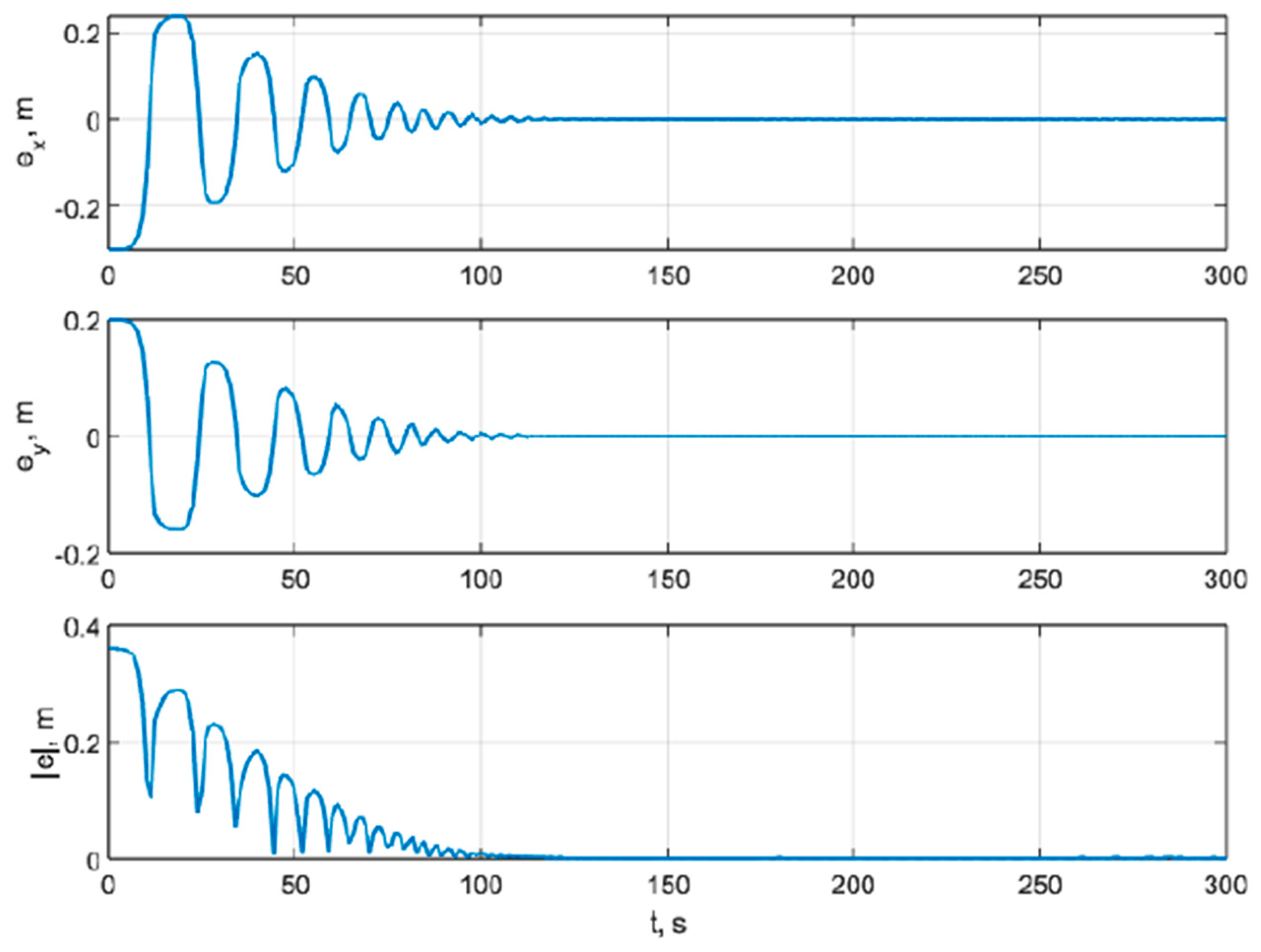
These plots confirm stability of the internal nonlinear loop and proper functioning of the linearized outer loop. The evolution of the position tracking errors is presented in Figure 17. The maximum transient deviations occur at the beginning of the motion due to the initial misalignment between the robot and the reference trajectory: maximum error in the x-direction: ≈ 0.22 m; maximum error in the y-direction: ≈ 0.25 m; maximum overall positional deviation: ≈ 0.28 m. These deviations decay rapidly, and by ≈ 120 s the tracking errors converge to zero. In the steady-state phase, the robot maintains sub-centimeter accuracy: m.
This figure clearly demonstrates the rapid error decay and excellent tracking precision achieved after convergence.
4. Discussion
The proposed trajectory-tracking method is closely related to the well-known CTC technique for serial manipulators, also referred to as inverse-dynamics control. At the conceptual level, both approaches rely on transforming a nonlinear plant via static-feedback linearisation into an equivalent trivial linear controllable system. As a result, the control problem for an nnn-dimensional nonlinear system reduces to the control of nnn independent one-dimensional decoupled linear subsystems. The resulting trajectory-tracking architectures are structurally identical: in both cases, a nonlinear inner loop performs linearisation, while a linear outer loop implements standard tracking laws using classical linear controllers. Consequently, together with the recognised advantages of CTC, which remains a highly active research area due to its excellent performance characteristics [26,27,28] the proposed method naturally inherits the limitations that are intrinsic to static-feedback linearisation.
A key drawback of CTC type methods is their limited robustness to model uncertainty: even small discrepancies between the real plant and the mathematical model used inside the linearising controller can lead to noticeable degradation of tracking performance. In this study, a simple kinematic DDWMR model was deliberately chosen to ensure transparency of the approach and ease of simulation. Nevertheless, our simulation experiments confirm the expected behaviour: the performance of the proposed controller is sensitive to parameter mismatches, similarly to classical CTC. This phenomenon is well-documented in the CTC literature, where modern research directions focus on adaptive and robust extensions, including the use of machine-learning-based compensation mechanisms [20].
Since the trajectory-tracking architecture proposed in this paper consists of two nested loops—a nonlinear inner loop that linearises the plant, and an outer loop that performs trajectory tracking of the linearised system—the outer loop can incorporate a wide range of modern control techniques, including robust, adaptive, optimal, or MPC-based controllers. This is a fundamental difference from most existing flatness-based methods for DDWMRs, which rely on approximate linearisation in the neighbourhood of a predefined reference trajectory (exact feedforward linearisation). Such schemes require a sufficiently accurate match between the initial state of the robot and the nominal initial condition of the reference trajectory, and they may exhibit performance loss or even instability in case the robot starts significantly away from the desired path.
By contrast, the method proposed here avoids these limitations because it performs plant linearisation, not trajectory linearisation. In other words, it is the nonlinear plant itself that is converted into an equivalent linear controllable system, rather than the entire trajectory-tracking closed loop. As highlighted earlier, current research trends increasingly focus on adaptive flatness-based techniques and on the application of MPC, optimal control, and hybrid control methods to flat systems [15,16,23,24,25]. Notably, many of these techniques become particularly effective and easier to implement when applied to differentially flat systems [20], making the proposed architecture compatible with a broad class of advanced control methods.
Another characteristic distinction of the proposed approach is that it yields a SISO (single-input–single-output) control structure for the linearised system. In contrast, most existing DDWMR trajectory-tracking methods rely on multivariable controllers with coupled control channels [25]. The SISO nature of the resulting linear system significantly simplifies controller design, tuning, and implementation, providing a conceptually straightforward yet highly effective solution.
5. Further Perspectives
Future research is expected to proceed in two directions. First, the proposed linearization-based trajectory-tracking method can be extended from the kinematic DDWMR model to its full dynamic model, as well as to other classes of mobile robots, including balancing robots, aerial vehicles, and multi-degree-of-freedom robotic platforms. Such generalizations would enable a broader assessment of the method’s applicability to complex nonlinear robotic systems. Second, an important avenue for further work is the development of robust and adaptive extensions of the proposed controller. Given its sensitivity to model uncertainties—an inherent limitation shared with classical computed torque control—future research will focus on designing robust, adaptive, and learning-enhanced compensation mechanisms that preserve the advantages of the linearized structure while improving resilience to parameter variations and external disturbances.
6. Conclusions
This work has presented a linearisation-based trajectory-tracking framework for differential-drive wheeled mobile robots, in which a nonlinear kinematic model is transformed via static-feedback linearisation into an equivalent SISO linear system. This transformation allows the nonlinear trajectory-tracking problem to be reformulated as a classical linear control task for two decoupled first-order subsystems, greatly simplifying the controller design while maintaining strong theoretical guarantees.
The proposed approach is conceptually related to com CTC and inherits its principal advantages: transparency of design, explicit control of the closed-loop dynamics, and high tracking accuracy for sufficiently well-modelled systems. Simulation results confirm these benefits: the robot successfully converges to the desired circular trajectory, achieving a maximum transient deviation of 0.28 m, a settling time of approximately 120 s, and a steady-state mean tracking error below 0.01 m. These results demonstrate that linearising the plant itself, rather than the trajectory-tracking loop, provides a simple yet powerful mechanism for achieving high-precision tracking in nonlinear mobile robots.
At the same time, as with CTC, the method exhibits sensitivity to modelling inaccuracies, highlighting the importance of further research into robustness and adaptation. Nevertheless, the proposed framework establishes a general and extensible foundation for trajectory-tracking control of differentially flat systems and demonstrates strong potential for both theoretical development and practical deployment.
Author Contributions
Conceptualization, D.A., A.Kr., and G.N.; methodology, A. Kr, G.N., and A.K.; software, A. Kr. and G.N.; validation, G.N., A.Kr., A.K., and D.A.; formal analysis, D.A. and T.H.; investigation, G.N., A.Kr., A.D., A.K., and D.A.; resources, D.A.; data curation, D.A.; writing—original draft preparation, G.N. and D.A.; writing—review and editing, D.A. and T.H.; visualization, G.N.; supervision, D.A. and T.H.; project administration, D.A.; funding acquisition, D.A. and T.H. All authors have read and agreed to the published version of the manuscript.
Funding
This research was funded by Ministry of Science and Higher Education of the Republic of Kazakhstan, grant number AP19679327.
Institutional Review Board Statement
Not applicable.
Informed Consent Statement
Not applicable.
Data Availability Statement
The data presented in this study are available on request from the corresponding authors.
Acknowledgments
This research was funded by the Ministry of Science and Higher Education of the Republic of Kazakhstan, grant number AP19679327 “Methods of machine learning for tasks of automatic control and inertial navigation of mobile robots”. T. Haidegger is a Consolidator Researcher, receiving financial support from the Distinguished Researcher program of Obuda University [38].
Conflicts of Interest
The authors declare no conflict of interest.
References
- Gao, J.; Li, Y.; Jin, J.; Jia, Z.; Wei, C. Design, Analysis and Control of Tracked Mobile Robot with Passive Suspension on Rugged Terrain. Actuators 2025, 14, 389. [Google Scholar] [CrossRef]
- Hu, H.; Long, D.; Liang, Y.; Wang, B.; Wang, X.; Su, R. Braking Control of Mobile Robots Using Integral Sliding-Mode Algo-rithm with Composite Convergence Regulation. Processes 2025, 13, 2887. [Google Scholar] [CrossRef]
- Banu, S.; Das, O.; Venkadeshwaran, K.; Gaurav, A.; Kapoor, T.; Pandey, N. Designing an Adaptive Control System for Robust Path Planning in Autonomous Mobile Robots. Multidiscip. Sci. J. 2025, 7, e2025ss0120. [Google Scholar] [CrossRef]
- Zeng, Z.; Chen, S.; Kong, X.; Li, X.; Zhang, C.; Yang, G. Revised Control Barrier Function with Sensing of Threats from Relative Velocity Between Humans and Mobile Robots. Sensors 2025, 25, 4005. [Google Scholar] [CrossRef]
- IEEE 24748-7000-2022; IEEE/ISO/IEC International Standard—Systems and Software Engineering—Life Cycle Manage-ment—Part 7000: Standard Model Process for Addressing Ethical Concerns During System Design. IEEE: New York, NY, USA, 2022.
- Houghtaling, M.A.; Fiorini, S.R.; Fabiano, N.; Gonçalves, P.J.S.; Ulgen, O; Prestes, E. Standardizing an Ontology for Ethically Aligned Robotic and Autonomous Systems. IEEE Trans. Syst. Man Cybern. Syst. 2023, vol. 54, 1791–1804. [Google Scholar] [CrossRef]
- Haidegger, T.; Mai, V.; Mörch, C.; Boesl, D.; Jacobs, A.; Khamis, A.; Lach, L.; Vanderborght, B. Robotics: Enabler and inhibitor of the sustainable development goals. Sustain. Prod. Consum. 2023, vol.43, 422–434. [Google Scholar] [CrossRef]
- Bloch, A.; Crouch, P.; Bailleul, J.; Marsden, J. “Nonholonomic Mechanics and Control” (Interdisciplinary Applied Mathematics); SpringerVerlag, New York, 2003. [Google Scholar]
- Luviano-Juárez, A.; Cortés-Romero, J.; Sira-Ramírez, H. Trajectory tracking control of a mobile robot through a flatness-based exact feedforward linearization scheme. J. Dyn. Syst. Meas. Control 2015, 137, 051003. [Google Scholar] [CrossRef]
- Chen, L.; Jia, Y. Variable-poled tracking control of a two-wheeled mobile robot using differential flatness. J. Robot. Netw. Artif. Life 2014, 1, 12–16. [Google Scholar] [CrossRef]
- Rigatos, G. Nonlinear Control and Filtering Using Differential Flatness Theory Approaches: Applications to Electromechanical Systems; Springer: Cham, Switzerland, 2016. [Google Scholar]
- Chen, L.; Jia, Y. Output Feedback Tracking Control of Flat Systems via Exact Feedforward Linearization and LPV Techniques. Int. J. Control Autom. Syst. 2019, 17, 606–616. [Google Scholar] [CrossRef]
- Nicolau, F.; Respondek, W.; Barbot, J.-P. Construction of flat inputs for mechanical systems. In Proceedings of the 7th IFAC Workshop on Lagrangian and Hamiltonian Methods for Nonlinear Control, Berlin, Germany, 18–21 October 2021. [Google Scholar]
- Nicolau, F.; Respondek, W.; Barbot, J.-P. How to minimally modify a dynamical system when constructing flat inputs? Int. J. Robust Nonlinear Control 2021, 31(18), 9538–9561. [Google Scholar] [CrossRef]
- Rodriguez-Guevara, D.; Favela-Contreras, A.; Beltran-Carbajal, F.; Sotelo, C.; Sotelo, D. A Differential Flatness-Based Model Predictive Control Strategy for a Nonlinear Quarter-Car Active Suspension System. Mathematics 2023, 11, 1067. [Google Scholar] [CrossRef]
- Li, Y.; Zhu, Q.; Elahi, A. Quadcopter Trajectory Tracking Control Based on Flatness Model Predictive Control and Neural Network. Actuators 2024, 13, 154. [Google Scholar] [CrossRef]
- Hamad, Q.M.; Raafat, S.M. A Flatness-Based Trajectory Tracking Control for Chemical Reactor. In Proceedings of the 21st In-ternational Multi-Conference on Systems, Signals & Devices (SSD 2024), Erbil, Iraq, 22–25 April 2024; pp. 819–825. [Google Scholar] [CrossRef]
- Lamraoui, H.C.; Bouzid, Y.; Nemra, A. Flatness-based nonlinear internal model control with disturbances compensation via improved extended state observer for remotely operated vehicle. International Journal of Control 2024, 98(6), 1480–1494. [Google Scholar] [CrossRef]
- Rigatos, G.; Wira, P.; Abbaszadeh, M.; Pomares, J. Flatness-based control in successive loops for industrial and mobile robots. In Proceedings of the 48th Annual Conference of the IEEE Industrial Electronics Society (IECON 2022), 2022; pp. 1–6. [Google Scholar] [CrossRef]
- Join, C.; Delaleau, E.; Fliess, M. Flatness-based control revisited: The HEOL setting. Comptes Rendus. Mathématique 2024, 362, 1693–1706. [Google Scholar] [CrossRef]
- Fliess, M.; Lévine, J.; Martin, P.; Rouchon, P. A Lie–Bäcklund approach to equivalence and flatness of nonlinear systems. IEEE Trans. Autom. Control 1999, 44, 922–937. [Google Scholar] [CrossRef]
- Sun, S.; Romero, A.; Foehn, P.; Kaufmann, E.; Scaramuzza, D. A Comparative Study of Nonlinear MPC and Differen-tial-Flatness-Based Control for Quadrotor Agile Flight. IEEE Transactions on Robotics 2022, vol. 38(no. 6), 3357–3373. [Google Scholar] [CrossRef]
- Beaver, Logan E.; Malikopoulos, Andreas A. Optimal control of differentially flat systems is surprisingly easy. Automatica 2024, 159, 111404. [Google Scholar] [CrossRef]
- Filho, J. O. Limaverde; Fortaleza, E. C. R.; Campos, M. C. M. A derivative-free nonlinear Kalman filtering approach using flat inputs. In International Journal of Control Taylor and Francis; 2021. [Google Scholar]
- Bröcker, Markus; Herrmann, Lukas. Flatness based control and tracking control based on nonlinearity measures. IFAC-PapersOnLine 2017, 50(Issue 1), 8250–8255. [Google Scholar] [CrossRef]
- Han, Y.; Ma, H.; Wang, Y.; et al. Neural Network Robust Control Based on Computed Torque for Lower Limb Exoskeleton. Chin. J. Mech. Eng. 2024, 37, 37. [Google Scholar] [CrossRef]
- Luo, R.; Hu, Z.; Liu, M.; Du, L.; Bao, S.; Yuan, J. Adaptive Neural Computed Torque Control for Robot Joints with Asymmet-ric Friction Model. IEEE Robotics and Automation Letters 2025, vol. 10(no. 1), 732–739. [Google Scholar] [CrossRef]
- Nguyen, Nguyet; Ba, Dang. A Computed Torque Controller for Robotic Manipulators Using Nonlinear Neural Net-work. 2022, 487–492. [Google Scholar] [CrossRef]
- Shadrin, G.; Krasavin, A.; Nazenova, G.; Kussaiyn-Murat, A.; Kadyroldina, A.; Haidegger, T.; Alontseva, D. Application of compensation algorithms to control the speed and course of a four-wheeled mobile robot. Sensors 2024, 24, 7233. [Google Scholar] [CrossRef]
- Krasavin, A.; Nazenova, G.; Alontseva, A.; Dairbekova, A. Tracking Control of a Two-Wheeled Mobile Robot Based on En-dogenous Linearization of the Dynamic Model. In Proceedings of the 2025 International Conference on Artificial Intelligence, Computer, Data Sciences and Applications (ACDSA), Antalya, Türkiye, 2025; pp. 1–6. [Google Scholar] [CrossRef]
- Kussaiyn-Murat, A.; Kadyroldina, A.; Krasavin, A.; Tolykbayeva, M.; Orazova, A.; Nazenova, G.; Krak, I.; Haidegger, T.; Alontseva, D. Application of discrete exterior calculus methods for the path planning of a manipulator performing thermal plasma spraying of coatings. Sensors 2025, 25, 708. [Google Scholar] [CrossRef]
- Alontseva, D. L.; Ghassemieh, E.; Krasavin, A. L.; Kadyroldina, A. T. Development of 3D Scanning System for Robotic Plasma Processing of Medical Products with Complex Geometries. Journal of Electronic Science and Technology 2020, Vol 18. No 3, 212–222. [Google Scholar] [CrossRef]
- Alontseva, D. L.; Ghassemieh, E.; Krasavin, A. L.; Shadrin, G. K.; Kussaiyn-Murat, A. T.; Kadyroldina, A. T. Development of Control System for Robotic Surface Tracking. International Journal of Mechanical Engineering and Robotics Research 2020, Vol. 9(No. 2), P. 280–286. [Google Scholar] [CrossRef]
- Lynch, K.M.; Park, F.C. Modern Robotics: Mechanics, Planning, and Control; Cambridge University Press: Cambridge, UK, 2017. [Google Scholar]
- Siciliano, B.; Sciavicco, L.; Villani, L.; Oriolo, G. Robotics: Modelling, Planning and Control; Springer: London, UK, 2009. [Google Scholar] [CrossRef]
- Takacs, A.; Haidegger, T. A method for mapping V2X communication requirements to highly automated and autonomous vehicle functions. Future Internet 2024, 16(4), 108. [Google Scholar] [CrossRef]
- Takacs, A.; Haidegger, T. Infrastructural requirements and regulatory challenges of a sustainable urban air mobility ecosystem. Buildings 2022, 12(6), 747. [Google Scholar] [CrossRef]
- Haidegger, T. P.; Galambos, P.; Tar, J. K.; Kozlovszky, M.; Zrubka, Z.; Eigner, G.; Rudas, I. J. Strategies and outcomes of building a successful university research and innovation ecosystem. Acta Polytechnica Hungarica 2024, Vol 21.(Issue 10), 13–35. [Google Scholar] [CrossRef]
Figure 1.
A hardware-implementable transformation of system into an equivalent control system via static state feedback.
Figure 1.
A hardware-implementable transformation of system into an equivalent control system via static state feedback.
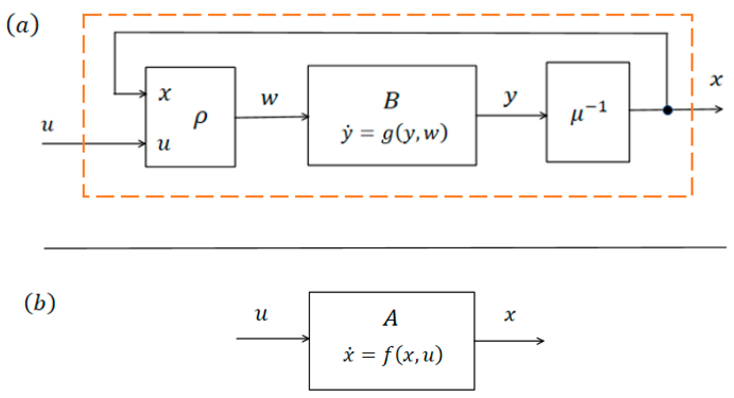
Figure 2.
Correspondence between the trajectories of equivalent control systems and , defined by the diffeomorphic mapping .
Figure 2.
Correspondence between the trajectories of equivalent control systems and , defined by the diffeomorphic mapping .
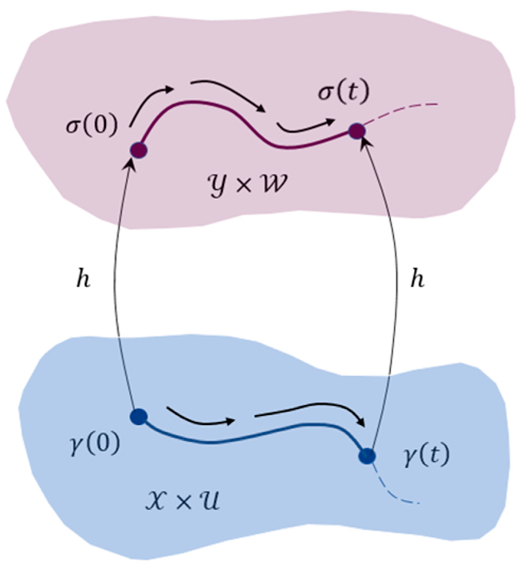
Figure 3.
Geometric parameters of the robot and its kinematic variables. Point (the nominal geometric center of the robot) lies at the intersection of the robot’s longitudinal axis of symmetry and the axis connecting the centers of the drive wheels.
Figure 3.
Geometric parameters of the robot and its kinematic variables. Point (the nominal geometric center of the robot) lies at the intersection of the robot’s longitudinal axis of symmetry and the axis connecting the centers of the drive wheels.
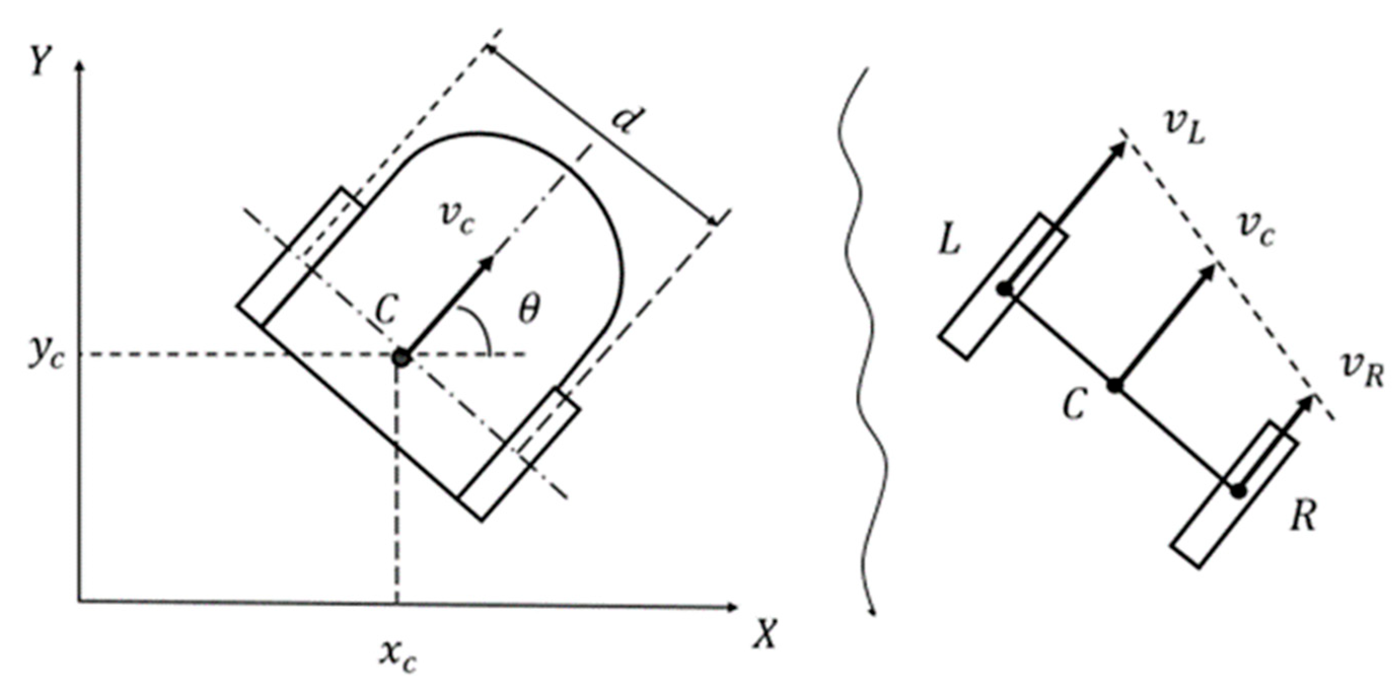
Figure 4.
Transformation of the differential-drive wheeled mobile robot kinematic model into model
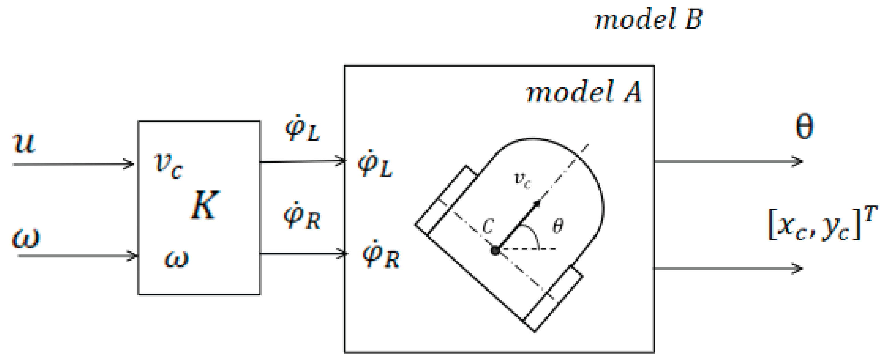
Figure 6.
Geometric interpretation of the coordinates on the manifold .
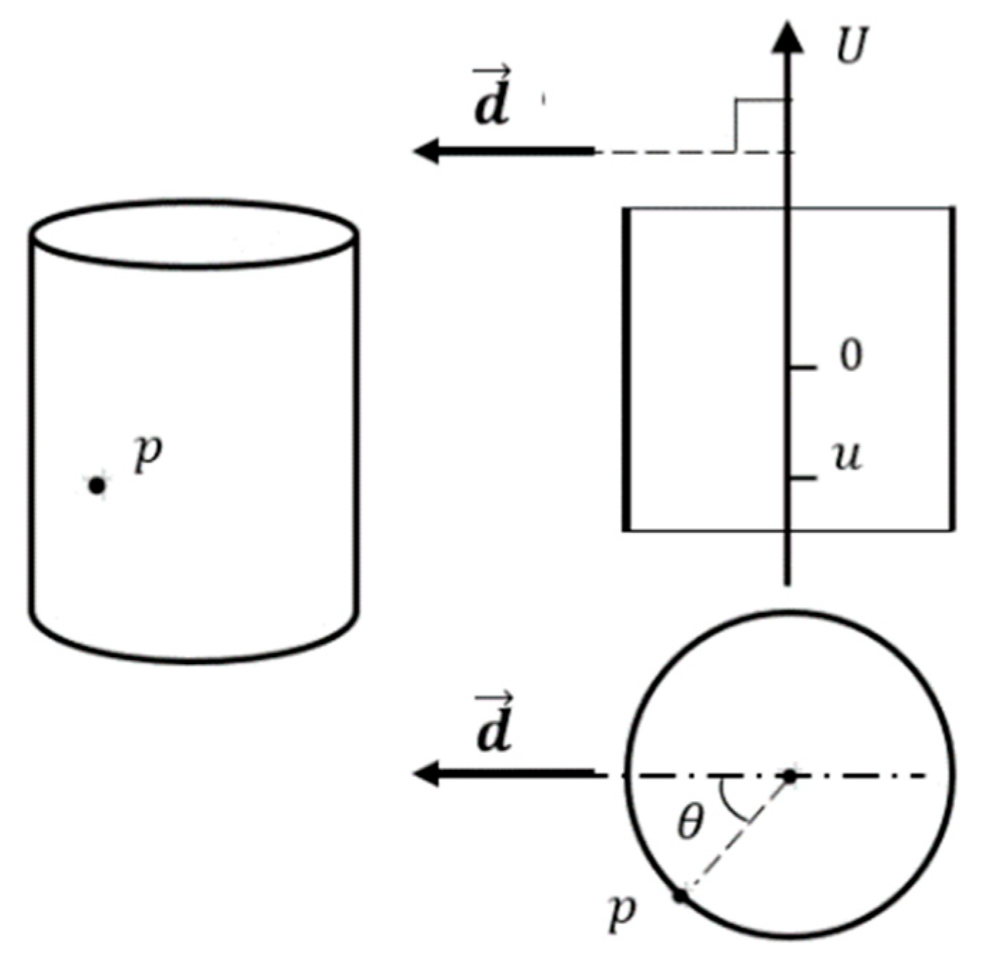
Figure 7.
The symmetry relation on the phase space induced by the automorphism .
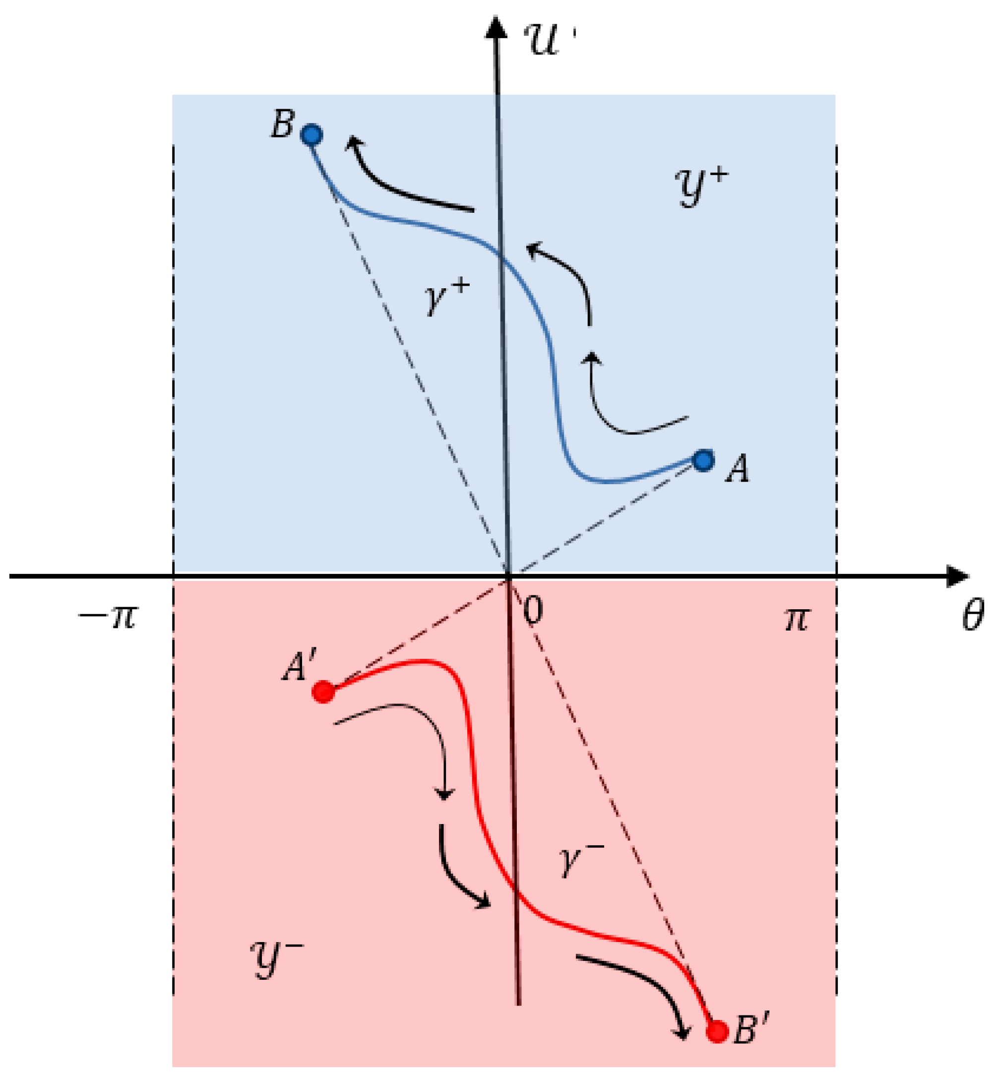
Figure 8.
Linearization scheme for the control system on the smooth manifold
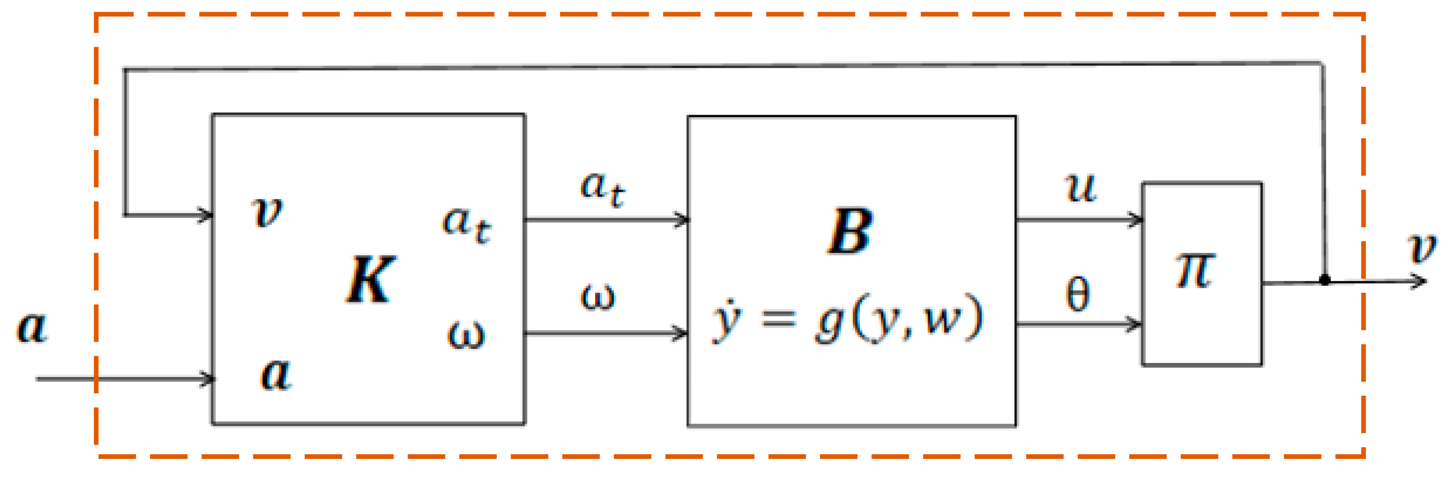
Figure 9.
Structural block diagram of the control system
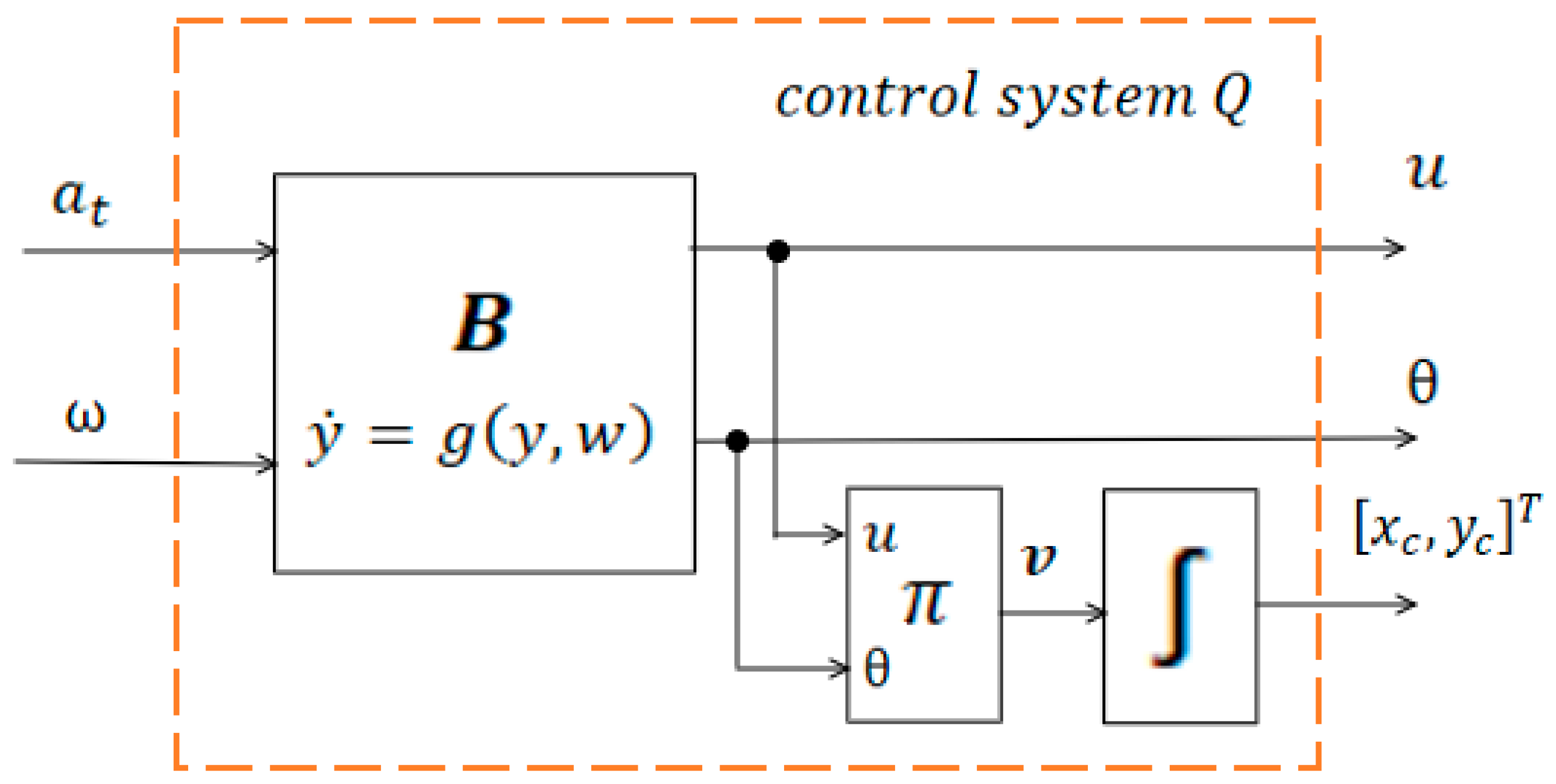
Figure 10.
Linearisation of the kinematic control system governing the motion of a point in the plane via static state feedback.
Figure 10.
Linearisation of the kinematic control system governing the motion of a point in the plane via static state feedback.
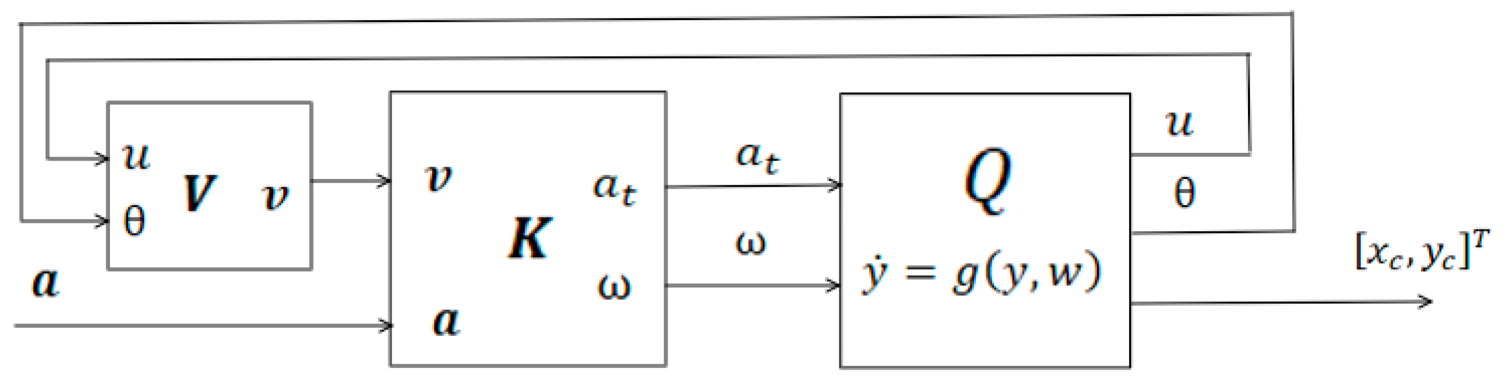
Figure 11.
Linearisation scheme for the simplest kinematic model of the DDWMR.
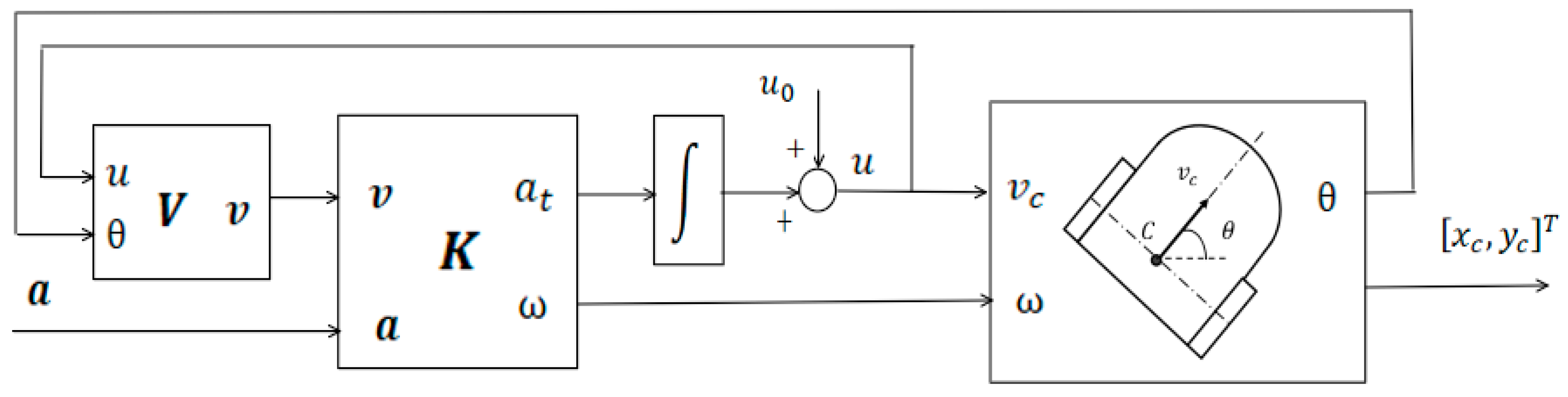
Figure 12.
(a) Equivalent representation of the linearised kinematic model of the DDWMR in the form of a chain of integrators. (b) Basic feedforward trajectory-tracking control scheme.
Figure 12.
(a) Equivalent representation of the linearised kinematic model of the DDWMR in the form of a chain of integrators. (b) Basic feedforward trajectory-tracking control scheme.
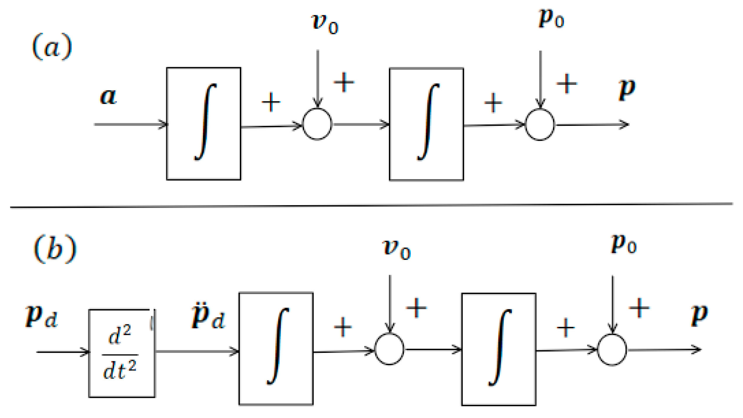
Figure 13.
Equivalent block diagram of the
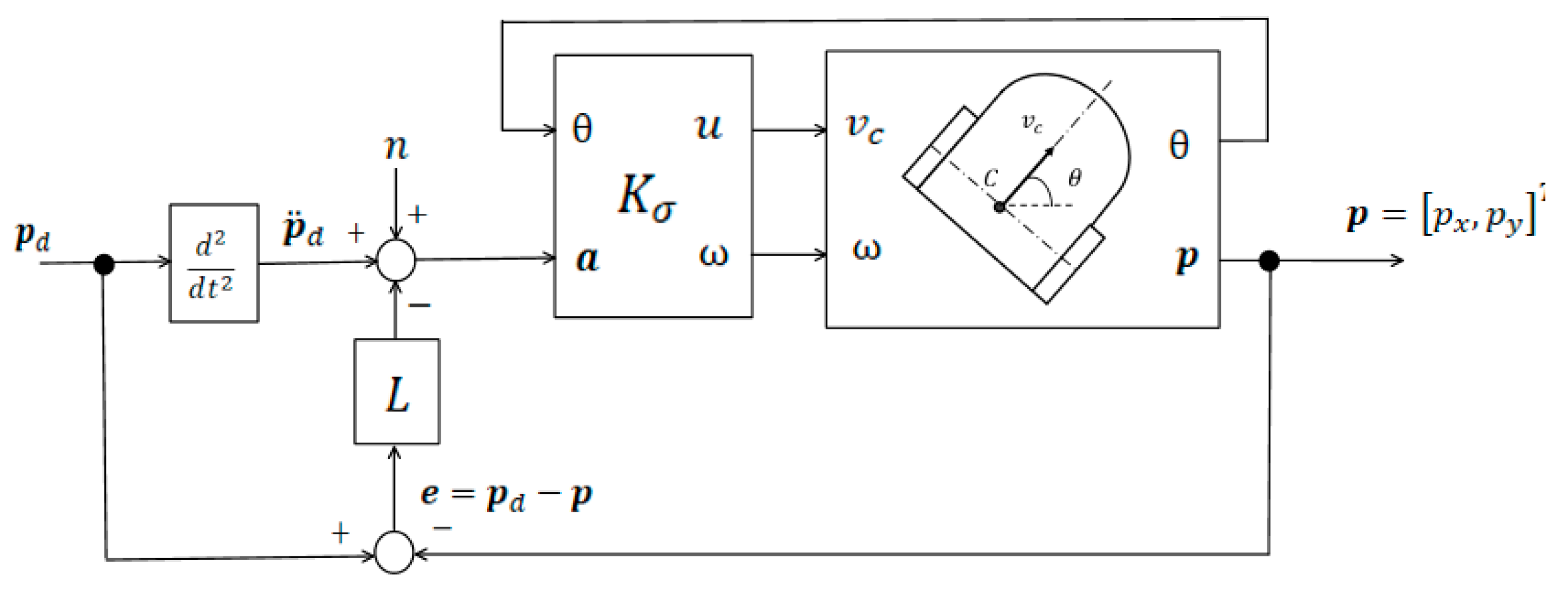
Figure 14.
Laplace-domain block diagram of the
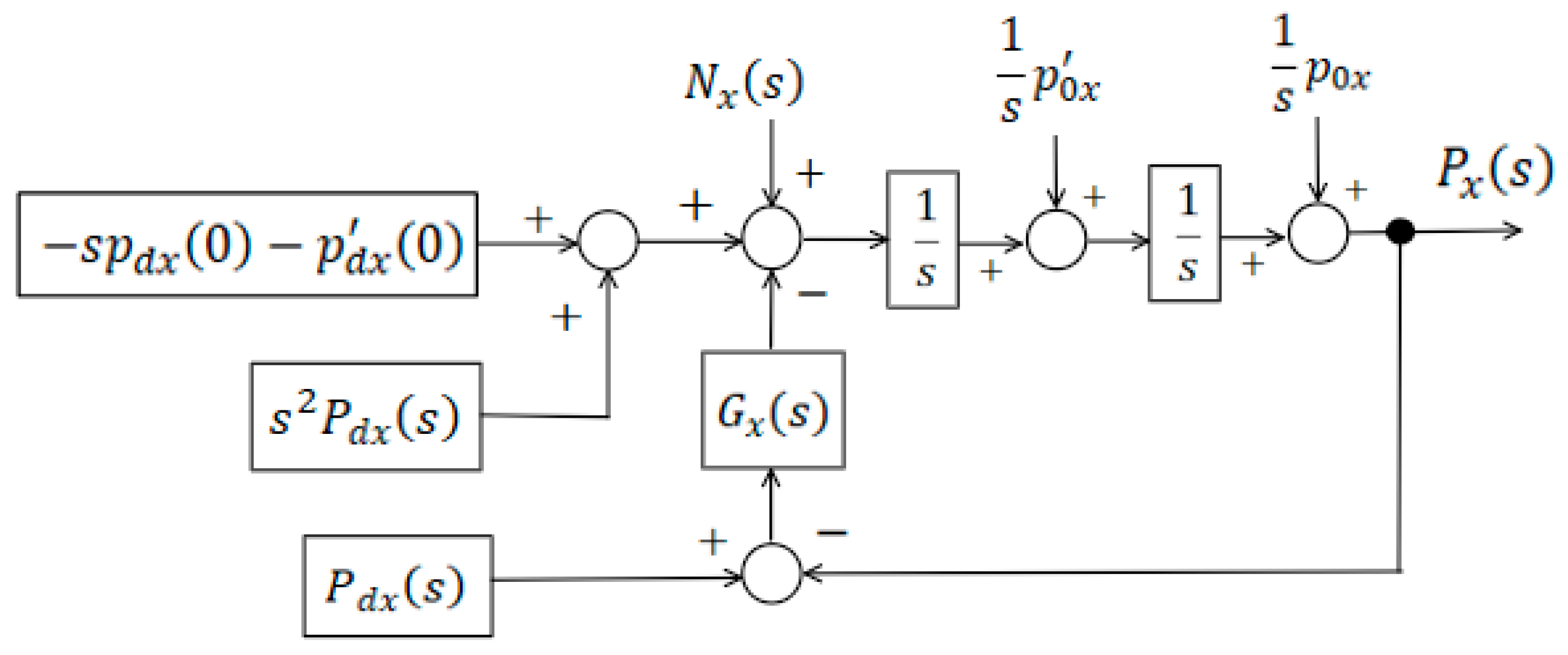
Figure 15.
Desired circular trajectory and actual robot trajectory during the simulation. The robot converges to the reference path and maintains accurate tracking in steady state.
Figure 15.
Desired circular trajectory and actual robot trajectory during the simulation. The robot converges to the reference path and maintains accurate tracking in steady state.
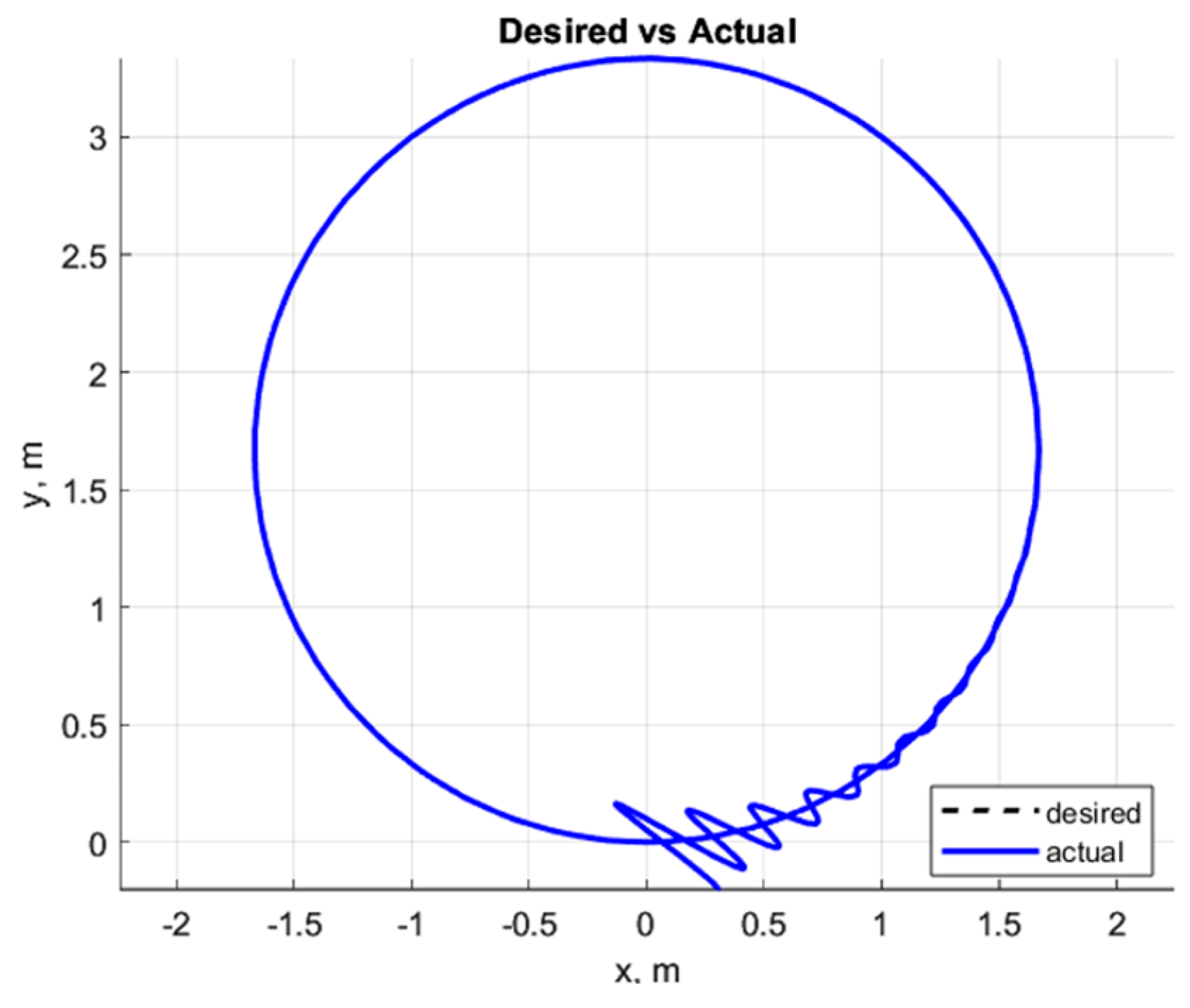
Figure 16.
Angular velocity and heading angle.
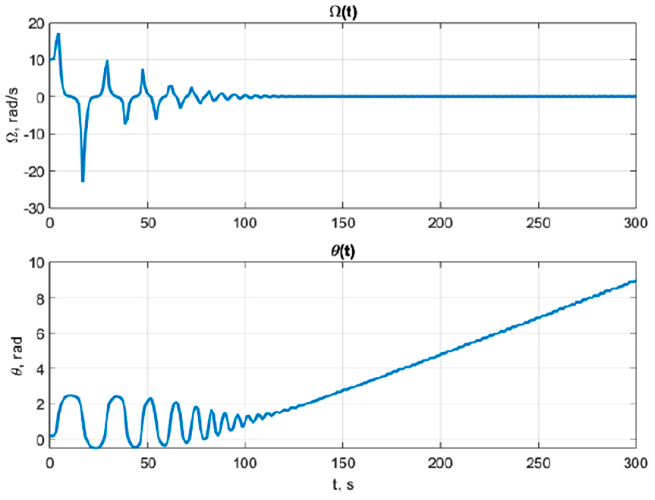
Figure 17.
Position errors in x, y, and absolute error.
Disclaimer/Publisher’s Note: The statements, opinions and data contained in all publications are solely those of the individual author(s) and contributor(s) and not of MDPI and/or the editor(s). MDPI and/or the editor(s) disclaim responsibility for any injury to people or property resulting from any ideas, methods, instructions or products referred to in the content. |
© 2025 by the authors. Licensee MDPI, Basel, Switzerland. This article is an open access article distributed under the terms and conditions of the Creative Commons Attribution (CC BY) license (http://creativecommons.org/licenses/by/4.0/).
Copyright: This open access article is published under a Creative Commons CC BY 4.0 license, which permit the free download, distribution, and reuse, provided that the author and preprint are cited in any reuse.


