
Submitted:
09 December 2025
Posted:
11 December 2025
You are already at the latest version
Abstract
Owing to changing climatic and environmental conditions, plant diseases are becoming increasingly prevalent, posing a serious threat to global agriculture. Timely and accurate diagnosis remains challenging, especially where scouting still relies on manual inspection. We propose B2-GraftingNet, a deep learning framework for automated detection of grape leaf diseases. B2-GraftingNet is a streamlined variant of our earlier B4-GraftingNet, retaining its strengths while simplifying blocks for faster inference and deployment. The architecture combines a VGG16 backbone with Inception-style blocks inside a custom CNN to extract robust, multi-scale features based on color, size, and shape. To reduce redundancy and improve generalization, Binary Particle Swarm Optimization (BPSO) selects informative features prior to classification. We evaluate Support Vector Machines (SVM) and k-Nearest Neighbors (KNN); a cubic SVM attains 99.56% peak accuracy on the public Kaggle grape-leaf dataset. For context, we also benchmarked standard pretrained CNNs on the same data, observing validation accuracies of 34.04% (VGG16), 34.04% (VGG19), 97.95% (Xception), 94.91% (Darknet), and 98.44% (ResNet-50); B2-GraftingNet matches or exceeds these while remaining lighter and faster to train and deploy. To enhance transparency and actionability, we pair Grad-CAM, LIME, and occlusion-sensitivity visualizations with a local gpt-oss:20b assistant (served via Ollama) that converts evidence into plain, grower-focused guidance and supports interactive chat validated by horticulturists. Results are further checked against expert-annotated ground-truth labels, confirming high accuracy and computational efficiency. Overall, B2-GraftingNet offers a reliable, interpretable, and scalable solution for early grape-leaf disease detection. The complete setup (code, model, web platform, configuration, and assets) is available on Zenodo: https://doi.org/10.5281/zenodo.17353656.
Keywords:
deep learning
; grape diseases
; binary particle swarm optimization
; XAI
; LLM assistance
1. Introduction
Grapevines (Vitis vinifera) rank among the world’s most widely cultivated fruit crops, underpinning a global industry valued at over USD 215 billion and contributing approximately 72.5 million tonnes in 2023, despite production challenges driven by extreme weather conditions and pest pressures (Intelligence 2024). Foliar diseases such as black rot, esca (black measles), leaf blight and downy mildew can each inflict yield losses ranging from 5 to 80%, depending on the severity and timing of infection (Guha 2025; Ploetz and Freeman 2009). Early and precise diagnosis of these diseases in vineyards is therefore a critical priority for sustaining both productivity and fruit quality.
Typically, vineyard health monitoring relies on field experts conducting visual inspections of leaves, shoots and clusters, a process that is inherently labor intensive, time consuming and subject to interoperator variability (Ammoniaci et al. 2021; Ferro and Catania 2023; Moreno Párrizas and Andújar 2023). As farm sizes expand and labour costs rise, manual scouting alone can no longer meet the demand for timely disease surveillance. This has spurred rapid advances in smart agriculture technologies, including unmanned aerial vehicles, multispectral imaging and Internet of Things (IoT) sensor networks, but translating raw field data into actionable disease alerts remains challenging under variable lighting, complex backgrounds and mixed phenological stages (Anastasiou et al. 2023; Dutta et al. 2025).
In recent years, considerable research efforts have been directed towards machine vision applications in agriculture, spanning a diverse range of areas, such as fruit maturity classification and quality rating (Olorunfemi et al. 2024), fruit disease diagnosis, plant pest identification (Habib et al. 2021), plant species classification (Kuan et al. 2025), fruit identification within harvesting robots (Hou et al. 2023), weed control and recognition (Upadhyay et al. 2024), and disease diagnosis and classification in plant organs (Mavridou et al. 2019).
The development of new models is facilitated by deep convolutional neural networks capable of directly processing images. Detecting plant diseases automatically under field conditions poses considerable challenges due to various factors, including complex backgrounds, natural lighting conditions, variations in plant phenological stages, and diverse symptom presentations (Minhans et al. 2025). The integration of cutting-edge technologies, including IoT (Jafar et al. 2024), big data analytics (S. Sharma et al. 2021), artificial intelligence (AI) (S. T. H. Shah et al. 2021; S. Sharma et al. 2021), remote sensing, satellite imagery, and UAVs (S. T. H. Shah et al. 2019; K. Sharma and Shivandu 2024), has propelled agriculture to new heights.
Cai et al. (Cai et al. 2023) introduced Siamese DWOAM-DRNet, an advanced deep learning model for classifying grape leaf diseases in complex natural scenes. Using an enhanced dataset of 1,209 images preprocessed with binary wavelet transform, variable thresholding, and Non-Local Means Multi-Scale Retinex (NL-MSR) (Li et al. 2022; Petro et al. 2014) optimization techniques, and further augmented for diversity, the model combines a Double-Factor Weight Optimization Attention Mechanism and a Diverse-Branch Residual Module for robust feature extraction. A joint loss function improved class separation and training convergence. The model achieved 93.26% accuracy and 93.23% F1 score, outperforming classical CNNs and recent methods, with added interpretability through Grad-CAM++ (Chattopadhyay et al. 2017) visualizations and strong generalization on external datasets.
Javidan et al. (Javidan et al. 2023) proposed an interpretable, machine vision-based method for grape leaf disease classification using the PlantVillage dataset, which targets black measles, black rot, leaf blight, and healthy leaves. Their pipeline combined K-means clustering for ROI segmentation, multi-color space feature extraction (GLCM, HOG, and LBP), PCA for dimensionality reduction, and Relief for feature selection, followed by classification with a linear SVM. The method achieved a high accuracy of 98.97%, surpassing the CNN and GoogLeNet (Szegedy et al. 2014) benchmarks, and maintained fast processing times. By ranking 30 key features, the approach ensures transparency and practicality for real-world deployment, especially in resource-constrained environments.
Subramanya and Parkavi (S G and A 2025) investigated deep learning-based automation for grape leaf disease diagnosis using EfficientNet variants (B0, B5, B7) trained via transfer learning on a large Kaggle dataset of 9,027 images covering black rot, esca, leaf blight, and healthy leaves. After preprocessing and data augmentation, EfficientNetB0 delivered the best performance, with 92.71% training accuracy and 96.73% validation accuracy, outperforming B5 and B7 while offering faster convergence and minimal overfitting, making it practical for resource-limited scenarios. Although the study did not report precision, recall, F1 score, or Cohen’s Kappa and lacked explainable AI integration, it demonstrated EfficientNetB0's strong potential for accurate grape disease classification, with recommendations for future real-world testing and extended training.
Kaur and Devendran (Kaur and Devendran 2024) presented a semi-automated grape leaf disease detection system that combines optimized K-means segmentation with Grey Wolf Optimization (Mirjalili et al. 2014); hybrid feature extraction (Law’s masks, GLCM, LBP, Gabor); and an ensemble of ANN, SVM, KNN, logistic regression, and Naïve Bayes classifiers. The PlantVillage dataset achieved 95.69% accuracy, outperforming traditional and CNN methods while maintaining interpretability through explicit feature use, although XAI tools such as Grad-CAM were not used. They highlighted plans for real-field adaptation and a web-based tool for farmers.
Despite substantial progress in image-based grape leaf disease recognition, many existing mobile or GUI-based systems still struggle to capture fine-grained, disease-specific patterns and rarely provide end-to-end, explainable support for growers. To address these gaps, we propose B2-GraftingNet, a hybrid framework inspired by B4-GraftingNet (S. A. H. Shah et al. 2025) that combines a customized CNN (VGG16 backbone with Inception-style branches) and Binary Particle Swarm Optimization (BPSO) to learn compact, discriminative feature representations. Classical classifiers trained on these optimized features, particularly a cubic SVM, achieve 99.56% accuracy with consistent precision and recall, surpassing several standard pretrained CNN baselines on the same dataset. Beyond accuracy, B2-GraftingNet integrates ROI-aware XAI (Grad-CAM, LIME, occlusion sensitivity) with a local language model (gpt-oss:20b via Ollama (OpenAI et al. 2025)) that converts multi-view explanations into concise, grower-friendly guidance, delivered through a lightweight, deployable web service.
Contributions:
- A.
- We introduce B2-GraftingNet, a hybrid framework inspired by B4-GraftingNet that integrates a customized CNN with metaheuristic optimization for reliable, automated detection of grape leaf diseases.
- B.
- We design a task-specific feature extraction scheme that combines a VGG16 backbone with Inception-style branch modules, producing a compact and discriminative deep feature space.
- C.
- We apply Binary Particle Swarm Optimization (BPSO) to select the most informative deep features, reducing redundancy and computational cost while preserving high separability for classical classifiers.
- D.
- We demonstrate, through comparisons with state-of-the-art learning techniques, that B2-GraftingNet achieves superior accuracy and efficiency for grape leaf disease recognition.
- E.
- We integrate ROI-aware XAI (Grad-CAM, LIME, occlusion) with a local language model (gpt-oss:20b via Ollama) and an end-to-end MATLAB + Flask + Ollama pipeline, delivering grower-focused guidance and deployable web services for practical field use.
The structure of this paper is organized as follows: Section 2 presents the materials and methodology used for the proposed grape leaf disease detection framework, detailing the data sources, preprocessing, model architecture, and feature optimization techniques. Section 3 discusses the experimental results and provides a comprehensive analysis highlighting the model’s performance and interpretability. Section 4 concludes the study by summarizing the key findings, contributions, and potential future directions.
2. Materials and Methodology
The proposed method comprises several stages to perform grape leaf disease classification. These stages include data collection, feature extraction, feature selection, and classification. The architectural design of the proposed methodology is illustrated in Figure 1. A hybrid approach, combining a VGG-16 (Simonyan and Zisserman 2015) and Inception-style branches (Szegedy et al. 2015), is adopted to enhance pattern recognition and feature extraction. Feature selection is employed to reduce computational overhead and redundancy. The resulting features are classified using supervised learning algorithms.
2.1. Data Availability
The proposed technique is evaluated on the publicly available grape-leaf dataset from Kaggle (Gundale 2020). The dataset includes 7122 training and 1805 testing RGB images (256 × 256 × 3) across four classes: black rot, esca, leaf blight and healthy (Table 1; Figure 2). The images are stored in class-specific folders, with 1888, 1920, 1722 and 1692 samples per disease class and 472, 480, 430 and 423 samples in the corresponding test sets, respectively.
2.2. Customized CNN-Based B2-GraftingNet
The core contribution of this work is B2-GraftingNet, a 49-layer CNN that combines a pretrained VGG16 backbone (for strong, low-/mid-level priors) with custom Inception-style branched modules (for multi-scale feature capture), followed by lightweight classification heads. The network integrates both linear and branched elements. In total it includes 18 convolutional layers, 5 max-pooling layers, 4 ReLU layers, 3 batch-normalization layers, 4 cross-channel normalization (CCN) layers, 2 fully connected layers, 1 dropout layer, and 1 class output layer. The input tensor has shape 227 × 227 × 3, as illustrated in Figure 3. The input layer is where the suggested network begins. The feature map was produced by the convolutional layer (ConvL1), which was the second layer. The suggested network begins with a convolutional ConvL-1 layer, after which the branched layer is embedded in the network. The branched (BL-1) layer comprises 10 layers divided into 2 further branches, each receiving input from the cross-channel normalization (CrossNorm-1) layer. The first branch contains ConvL-2, LeakyReLU-1, ConvL-3, LeakyReLU-2, and ConvL-6. Figure 3 depicts the branched layer embedded in the CNN network. In the branched layer, feature maps were generated via parallel processing. The outputs of these branches were concatenated by the addition (Addition-1) layer.
After branched layer-1, some layers were connected sequentially via batch normalization (BatchNorm-1), ConvL-7, BatchNorm-2, MaxPool-1, and ConvL-8 layers. The second cross-channel normalization (CrossNorm-2) layer generated the input for the second branched layer. BL-2 was similar to BL-1, with the same number of layers in the same order. All the layers in BL-2 merged in the addition (A_2) layer. The output of the addition-2 layer passed to the next sequence, which contained MaxPool-2, CrossNorm-3, MaxPool-3, ConvL-14, BatchNorm-3, ConvL-15, ReLU-1, CrossNorm-4, ConvL-16, ReLU-2, MaxPool-4, ConvL-17, ReLU-3, ConvL-18, ReLU-4, MaxPool-5, FC-1, ReLU-5, Dropout FC-2, SoftMax, and Class Output. The proposed CNN had 2 fully connected (F.C.) layers, 2 dropout layers, 1 SoftMax (S) layer, and 1 output (class output) layer. A mathematical overview and the outputs of various levels of the customized CNN network were presented. An image or feature map I(Ijj−1) with kj channels was accepted as input by the convolutional layer, where j denotes the number of layers in the convolutional layer (51).
The output of the layer contains channels, and all of the channels in this layer are computed via equation (1).
where denotes the convolution operation. The term refers to the filter (or kernel) with a depth corresponding to , and represents the bias term for the channel. The nonlinear activation function is applied elementwise to the resulting feature map. The network employs two types of activation functions: the standard Rectified Linear Unit (ReLU) and the Leaky ReLU, as described in (52).
The ReLU layer converts all the negative values to zero by equation 2 as follows:
where and represent the image matrix I, which has a certain number of rows and columns. The leaky ReLU has a slight curve for the value 0 instead of beginning at zero. A leaky ReLU can have when the value of is less than zero.
Batch Normalization (B.N.) is a technique applied to each small batch in a neural network to standardize the inputs to a layer, thereby improving training speed and stability. It involves computing the batch mean and batch variance for each feature. The batch mean is calculated using the equation (3):
where denotes the feature in the batch and where is the total number of features in the batch. The batch variance is then computed via equation (4) as follows:
which quantifies the spread of the features around the batch mean.
Afterward, the features are normalized via equation (5) as follows:
where is the normalized feature, which is the batch mean, and where is the batch variance, which is a small constant added for numerical stability. To retain the network’s expressive capacity, two learnable parameters, and , are introduced to scale and shift the normalized values, respectively (53). This gives the final output in equation (6) as:
where and are learned during training.
The cross-channel normalization (CCN) layer is inspired by findings in neuroscience, where it has been observed that active neurons tend to inhibit the activity of their neighboring neurons. In the context of deep learning, this translates to suppressing feature responses across channels rather than within a single feature map. In the CCN, the “neighbor” refers to adjacent channels, and normalization is applied across these channels. Mathematically, CCN is expressed in equation (7) as:
where is the normalized activation at spatial location for channel and where is the original activation before normalization. The summation runs over a set of neighboring channels centered around channel , with indicating the number of channels included in the normalization window. N is the total number of channels in the layer. The parameters , , and are hyperparameters that control the normalization behavior: κ provides numerical stability, α scales the influence of surrounding channels, and determines the degree of normalization applied. The architectural diagram of the customized CNN-based model is shown in Figure 3.
B2-GraftingNet was explicitly designed to avoid ad-hoc or unstable combinations of heterogeneous modules. The network adopts a single, coherent tensor pipeline in which all convolutional blocks, including the Inception-style branches, operate on feature maps that share compatible spatial dimensions and channel depths. Specifically, the early convolutional stages follow the VGG16 design (stacked 3×3 kernels with stride 1 and max-pooling) to provide strong low- and mid-level priors. The Inception-style branched modules (BL-1 and BL-2) are then inserted at intermediate depths and are fed by cross-channel normalized feature maps. Each branch applies parallel convolutions with different receptive fields (1×1 and 3×3) and non-linearities, after which the branch outputs are concatenated along the channel dimension following an Addition/Concatenation layer that preserves the spatial resolution. This ensures that feature fusion is mathematically well-posed and does not require any ad-hoc reshaping or interpolation. In practice, we observed stable training behaviour with no exploding or vanishing activations, and ablation experiments in which branched modules were removed consistently reduced validation accuracy, confirming that the proposed hybrid backbone contributes complementary multi-scale information rather than introducing architectural instability.
In addition, all convolutional and fully connected layers in B2-GraftingNet are initialized with variance-scaled (He-style) random weights, which are well suited for ReLU-type activations and help avoid early saturation. The network uses a controlled combination of ReLU and Leaky ReLU units: standard ReLU is applied in deeper layers to promote sparsity, while Leaky ReLU is used in the Inception-style branches to mitigate dead-neuron effects. Batch-normalization layers are inserted at key depths to stabilize the distribution of activations during training and to allow the use of a relatively higher learning rate without divergence. To prevent overfitting, we employ multiple regularization mechanisms: (i) L2-weight decay on all trainable parameters, (ii) dropout in the fully connected block before the final classifier to decorrelate co-adapted features, and (iii) early stopping based on validation accuracy. Together with 10-fold cross-validation, these design choices provide a theoretically grounded and practically stable CNN configuration rather than a purely empirical or unregularized architecture.
2.3. Deep Network for Feature Extraction
B2-GraftingNet is trained on the grape leaf dataset using ADAM (Kingma and Ba 2015) optimizer with a learning rate of 0.01, momentum of 0.9, mini-batch size of 20, and 30 epochs (Table 2). After training, we use the second-to-last fully connected layer (fc_2) of B2-GraftingNet as a generic descriptor of grape-leaf appearance. This layer sits immediately before the final SoftMax classifier and therefore encodes high-level, class-discriminative information while remaining independent from the specific output layer weights. For each image, fc_2 produces a 1×1000 feature vector; stacking all samples results in an N × 1000 matrix that serves as input to the feature selection and classical classification stages, as described in Table 3. Prior to BPSO, all feature dimensions are standardized (zero mean, unit variance) to remove scale effects.
2.4. Feature Selection via Binary Particle Swarm Optimization (BPSO)
Feature selection is used to select those features from the feature set that are related to the highest predicted value. This work selects the optimized features via a nature-inspired-based algorithm called binary particle swarm optimization (BPSO) (Schutte and Groenwold 2005), as illustrated in Figure 4. In this algorithm, each particle is influenced by its velocity, and PBEST (personal best) provides the best position achieved by the whole swarm GBEST (global best), where GBEST = {g1, g2, g3, …, gn}. In the search space, the movement of particles is overseen by position and velocity updating, where the related equations are given below (Jiang et al. 2007). The velocity was computed via equations (9) and (10):
where and represent the velocity and position of the particle at iteration , respectively. The parameter is the inertia weight that controls the influence of the previous velocity. Constants and are cognitive and social coefficients, respectively, whereas and are uniformly distributed random numbers in the range . The term denotes the PBEST of the particle and s the GBEST achieved by the swarm at iteration . The function maps velocity to a probability between 0 and 1, and is a random number used to decide the binary position (0 or 1) of the particle.
In BPSO, the position of each particle is represented in a binary string with a fixed value of 0 or 1, and the velocity (V) represents the value of the probability of particles with a value of 1. The sigmoid function is introduced to transform the velocity value into the range of 0-1. In the BPSO technique, the position of the particle is updated according to equation (11) below.
where is the updated position of the particle at iteration and where is its velocity. The function is defined as and converts the velocity into a probability in the range . The term is a random number drawn from a uniform distribution in , and is the Heaviside step function, which returns a value of 1 if and 0 otherwise.
To enhance reproducibility, we explicitly specify the BPSO configuration used for feature selection. Each particle encodes a binary mask over the -dimensional deep feature vector, where a value of 1 indicates an active feature. The fitness function jointly optimizes classification performance and feature sparsity and is defined as in equation (12):
where is the 10fold cross-validation accuracy of a cubic SVM trained on the selected features, is the binary mask, is the number of selected features, is the full feature dimensionality (e.g., deep features), and is a small regularization constant that discourages overly large subsets.
The BPSO algorithm predicted the 1 × 750 dimensions of the feature for every single sample. These selected features contained the highest intensity pixel value to generate better classification results. The selected feature was passed to the supervised machine learning algorithm for further processing.
2.5. Supervised Machine Learning Classification
Images of grape leaf disease were accurately classified via a variety of supervised machine learning techniques. The SVM (Cortes and Vapnik 1995) and KNN classifiers (Cover and Hart 1967) served as the bases for the applied classifiers. In addition, SVMs exhibit the following variations: cubic SVMs (C-SVMs), fine Gaussian SVMs (FG-SVMs) (Liu et al. 2011), medium Gaussian SVMs (MG-SVMs), quadratic SVMs (Q-SVMs), linear SVMs (L-SVMs), and coarse Gaussian SVMs (CG-SVMs) (61). The cosine KNN (C-KNN), coarse KNN (CR-KNN), and fine KNN (F-KNN) (62) KNN classifiers and their sub-classifiers were used to validate the suggested approach.
3. Results and Discussion
The experimental results were compiled by a computed machine that contains several specifications: Windows 11 with a 5th generation computer and an NVIDIA RTX 2060 GPU with 8 GB of RAM. All the program-based commands are executed in the MATLAB2023a tool. For the classification results, this study uses different parameters, including accuracy (ACCU), precision (PREC), recall (RECL), kappa (KAPA), and the F1 score. A confusion matrix computes all these parameters. The mathematical formulas of all the parameters are given in equations (13)-(17):
3.1. Training of the Proposed CNN
The public Kaggle grape-leaf dataset provides a fixed train/test split (7,122 training and 1,805 test images across four classes), which we respect to enable fair comparisons with prior work. Within the training partition, we monitor accuracy and loss over iterations and use an internal train-validation split (70:30) to guide CNN training and hyperparameter selection, while the held-out Kaggle test set is never used for tuning and serves only to assess final generalization performance. To benchmark B2-GraftingNet, we fine-tuned standard pretrained CNNs on the same data and obtained the following validation accuracies: VGG16 34.04%, VGG19 34.04%, Xception 97.95%, Darknet 94.91%, and ResNet-50 98.44%. B2-GraftingNet achieves competitive accuracy while being significantly lighter and less complex, requiring lower compute and memory as well as shorter training and inference time, making it easier to embed in real-world applications, although we acknowledge that all results are obtained on a single curated dataset and that external validation on independent vineyards, cultivars, and seasons remains an important next step.
The proposed B2-GraftingNet model was trained on this split and demonstrated high generalizability across unseen data, while the trained model is available here (S. A. H. Shah et al. 2025). After training, the validation accuracy is 98.11%. Figure 5 shows the training accuracy, training loss, and parameters, respectively. The training graph depicts the learning behavior of the network with validation accuracy. After successful training, we removed the last Softmax layer and started to retrieve the feature vector at the 2nd fully connected (FC) layer of the CNN. Compared with existing methods, the proposed methodology achieves more efficient results. The suggested CNN-based network obtained optimized features that generate a better classification accuracy rate.
The BPSO algorithm was used to obtain an optimized feature set for the feature optimization process. All the experiments and their associated information are summarized in Table 4. Further, 10-fold cross validation was applied on the training dataset to identify the best model based on optimized features’ validation performances. Based on that, this study encompasses four distinct experiments for grape leaf disease detection and classification. All observations are rooted in the B2-GraftingNet CNN, and an optimized feature set.
Across the four observations, as detailed in Table 4, using the full B2-GraftingNet feature set (1,000 deep features per image; 1,805×1,000 matrix) already yields strong performance (98.78%, Obs-1). Applying BPSO to select a compact subset preserve (and in cases improves) accuracy while drastically reducing dimensionality. With an aggressive reduction to 100 features (Obs-2), accuracy remains essentially unchanged (98.615%), indicating substantial redundancy in the original representation and validating BPSO’s ability to keep the most discriminative cues. As the optimized budget increases to 500 and 750 features (Obs-3/Obs-4), performance climbs to 98.73% and 99.56%, respectively surpassing the unoptimized baseline at 750 features. Taken together, Table 4 shows that BPSO provides an advantageous accuracy efficiency trade-off: a 10× reduction (1,000 to 100) retains accuracy for lightweight deployments, whereas a moderate budget (~750) achieves the best observed score (99.56%) with far fewer features than the raw model, reducing compute/memory overhead and the risk of overfitting while maintaining or improving classification quality. The applied classifiers and their analysis parameters are briefly mentioned in Table 5 and Figure 6.
The detailed ablation study of B2-GraftingNet, including the impact of progressively reducing network depth, is provided in the Supplementary Manuscript (Section S1: Ablation Study of B2-GraftingNet).

Table 6.
Results comparison with those of existing methods.
| Study | Classifier | Accuracy (%) | Precision (%) | Recall (%) | Kappa | XAI |
| (Cai et al. 2023) | Siamese DWOAM-DRNet | 93.26 | 93.23 | 93.23 | - | Grad-CAM++ |
| (Javidan et al. 2023) | SVM (Linear) | 98.97 | - | - | - | Feature selection & ranking |
| (S G and A 2025) | EfficientNetB0 | 96.73 | - | - | - | None |
| (Kaur and Devendran 2024) | Ensemble (ANN, SVM, etc.) | 95.69 | - | - | - | None |
| Our Method | B2-GraftingNet + Cubic SVM | 99.56 | 99.58 | 99.58 | 0.99 | Grad-CAM + Activation Maps |
3.2. Optimum Results
This research involves multiple observations according to the number of optimized feature sets and different CNN networks. The highest optimized result is in observation #4, with 750 selected grape leaf disease dataset features having 1805 images. We used deep feature extraction the BPSO algorithm for optimized feature selection. The highest performance was achieved in observation #4, where the cubic SVM classifier attained an accuracy of 99.56% when the optimally selected feature set was used. Among all observations, this result corresponds to the best configuration, which employs an optimized feature matrix with dimensions of 1805 × 750. The confusion matrix and ROC curve of the experimental classes are shown in Figure 7, and Figure 8. The SVM, KNN, and several kernel functions achieved the highest accuracy in our proposed methodology. The performance of the method associated with observation 4 was better than that of the other prediction rates.
3.3. Comparison with Previous Studies
A comprehensive comparison of recent grape leaf disease detection methods reveals the strengths and limitations of various approaches in terms of classification accuracy, interpretability, and model robustness. Cai et al. (Cai et al. 2023) introduced the Siamese DWOAM-DRNet, a novel deep architecture that achieved an accuracy of 93.26% with balanced precision and a recall of 93.23%. Their model leveraged advanced attention mechanisms and explainability through Grad-CAM++, which highlighted disease-relevant regions, offering interpretability in real-world scenarios. In contrast, Javidan et al. (Javidan et al. 2023) adopted a machine vision-based method using a linear SVM classifier, which yielded a remarkably high accuracy of 98.97%. While they did not report precision, recall, or kappa metrics, their approach stood out for its use of interpretable handcrafted features and ranking-based feature selection, promoting transparency over deep neural networks.
Subramanya and Parkavi (S G and A 2025) evaluated EfficientNet variants and reported that EfficientNetB0 performed best, achieving 96.73% accuracy. Although this lightweight model offered a good balance of efficiency and accuracy, the study did not incorporate explainability tools, limiting its interpretability. Kaur and Devendran (Kaur and Devendran 2024) presented a hybrid ensemble approach that combines multiple classifiers and achieved 95.69% accuracy. Despite its competitive performance, the absence of explainable AI tools has reduced its practical diagnostic value.
In contrast, the proposed B2-GraftingNet framework, combined with the cubic SVM, outperforms all prior methods, with an exceptional accuracy of 99.56% and precision and recall scores of 99.58%. Additionally, a kappa score of 0.99 was reported, indicating strong agreement with the expert-labelled ground truth. The integration of Grad-CAM and activation map visualization further distinguishes it by providing meaningful interpretability and transparency, confirming its potential for practical deployment in real-field agricultural settings.
3.4. Explainable AI Results
3.4.1. Visualization of Different Activation Layers via the Customized CNN Model
After the customized CNN learns, we analyse the feature mapping of different convolutional layers on grape leaf disease and observe the pixels activated by the customized CNN model. Figure 9 presents the hierarchical visualization of feature maps generated at various convolutional layers of the customized CNN model. The subfigures, labelled from (i) to (xiii), correspond to outputs from selected convolutional layers: convL1 through convL18. At early layers such as convL1 to convL4 (i-iv), the network captures low-level features such as edges, textures, and color gradients. These layers exhibit high visual clarity and focus on generic spatial patterns of grape leaves, which is useful for forming foundational representations. In the intermediate layers, convL5 to convL8 (v-viii), the filters begin to extract more abstract features. These include mid-level patterns such as disease patches, shape deformations, and vein distributions, demonstrating the transition from general to class-specific attributes. The deeper layers, convL14 to convL18 (ix-xiii), show increasingly sparse and high-level activations. While the raw texture visibility is reduced, these layers encode high-dimensional abstract representations that are highly specific to classification tasks. In particular, convL16 and convL18 show minimal but sharp activations, likely corresponding to distinctive disease symptoms or healthy traits learned by the network. This Figure 9 collectively illustrates the model’s ability to progressively abstract input information layer by layer from basic edge detectors to highly selective patterns relevant for disease classification in grape leaves.
3.4.2. Visual Explanations via Grad-Cam from the Customized CNN Model
The Grad-CAM (gradient-weighted class activation mapping) (Selvaraju et al. 2017) function is used to visualize the target region from the input image. This method represents the trained customized CNN model's validity and visual explanation and generates a heatmap of the focused area. Figure 10 displays the results applied to the output of the customized CNN, with each column corresponding to a different class: Black_rot, Esca, Leaf_blight, and healthy. The top row shows the original grape leaf images from each class. The bottom row shows the Grad-CAM heatmaps superimposed on the original leaves, highlighting the most influential regions contributing to the model’s predictions. In these heatmaps, the red and yellow areas represent regions with high activation, indicating where the model concentrates its attention to make a decision, whereas the blue areas denote regions with low activation, indicating minimal relevance to the classification process. For disease categories such as Black_rot, Esca, and Leaf_blight, the Grad-CAM outputs effectively localize disease-specific symptoms, including lesions, discolouration, and necrotic patterns. In contrast, for the healthy class, the model focuses broadly on the entire leaf structure due to the absence of disease markers. Overall, these visualizations enhance interpretability and demonstrate that the CNN reliably identifies relevant disease features rather than being misled by irrelevant background details, thus confirming the transparency and effectiveness of the model’s learning process.
The proposed B2-GraftingNet model offers significant benefits for practical agricultural applications by enabling fast, accurate, and interpretable diagnoses of grape leaf diseases. Its integration of explainable AI techniques, such as Grad-CAM, further strengthens its applicability by providing visual insights into the decision-making process. In addition to delivering high accuracy and transparency, B2-GraftingNet is highly adaptable and reusable: the extracted feature representations can be easily transferred to detect and classify other plant leaf diseases and even adapted to diagnose other agricultural disease problems beyond grapes. Furthermore, the robust architecture and flexible feature extraction framework can be extended to address classification tasks in non-agricultural domains, such as medical imaging, environmental monitoring, and industrial inspection. The lightweight, modular design enables seamless integration with mobile or edge devices, making it practical for in-field, real-time use by farmers, agronomists, and experts across various domains. This unique combination of flexibility, transferability, and interpretability makes B2-GraftingNet a versatile, high-impact solution for modern precision agriculture and a wide range of intelligent digital diagnostics.
3.4.3. Web Platform, Model, and LLM Assistance
The LLM component is not used for disease classification; instead, it consumes ROI-aware XAI summaries and produces human-readable guidance. For each analysed image, we aggregate Grad-CAM, LIME, and occlusion metrics into a short textual context describing (i) the predicted class and confidence, (ii) where the network focuses on the leaf, and (iii) qualitative agreement between methods. This context is passed to a local large language model via a fixed prompt that enforces four sections (“Verdict”, “Where to look”, “What to do now”, “Caution”) and explicitly forbids numerical claims or treatment recommendations beyond standard hygiene and scouting practices.
To assess the practical utility of the assistant, two experienced horticulturists independently examined a stratified sample of outputs covering all disease classes and both clear and borderline cases. They rated each message for clarity, agronomic plausibility, and safety and suggested minor wording adjustments, which we integrated into the prompt and post-processing rules. The examiners agreed that the assistant effectively points growers towards relevant leaf regions, avoids over-confident prescriptions, and remains consistent with the underlying XAI evidence. Because all processing is performed locally (MATLAB + Flask + Ollama) and images are not transmitted to external services, the assistant can be safely deployed in privacy-sensitive or offline field settings.
The Supplementary Materials contain full implementation details for our end-to-end system, including (i) the web platform (S. B. H. Shah et al. 2025a) (UI layout, routes, REST API schema, request/response examples, and deployment notes), (ii) the vision model pipeline (B2-GraftingNet architecture (S. B. H. Shah et al. 2025b) combining VGG16 and Inception branches, and BPSO selection, training/validation splits, hyperparameters, and export format), and (iii) the local LLM assistant (prompt design, grounding from ROI-aware Grad-CAM/LIME/Occlusion summaries, chat context injection, and safety constraints). We also provide step-by-step setup instructions (installing Ollama, pulling gpt-oss:20b, environment variables), a configuration YAML for reproducible runs, API examples for mobile image uploads and programmatic retrieval of classifications, explainability overlays, and assistant insights, as well as additional figures and code listings that mirror the production repository.
4. Conclusion
In this research, the main contribution lies in the introduction of a novel deep learning model named B2-GraftingNet, which incorporates a customized CNN-based feature extraction framework. The model is first trained on the Kaggle grape-leaf disease dataset and then evaluated on the same public benchmark. Feature matrices extracted by the pretrained network are optimized with Binary Particle Swarm Optimization (BPSO), and selected subsets are classified using SVM and KNN under 10-fold cross-validation. Among six evaluation setups, cubic SVM attains 99.56% accuracy with a fused, BPSO-optimized set of 750 features, while medium Gaussian SVM reaches 99.45% with the same feature budget showing that the number of selected features meaningfully influences performance across classifiers. Beyond accuracy, we pair the vision system with a local language model (gpt-oss:20b via Ollama) that converts ROI-aware Grad-CAM/LIME/Occlusion evidence into plain, field-ready guidance and supports interactive chat. This on-device assistant preserves privacy, works offline, and was qualitatively validated by two horticulturists, who confirmed that the generated advice is actionable for growers. Overall, B2-GraftingNet, combined with grounded gpt-oss assistance, delivers a fast, accurate, and interpretable pipeline for early grape leaf disease detection and decision support.
The proposed methodology can be extended to other plant species and leaf-disease datasets to validate generalizability. We will also evaluate performance on strictly held-out, never-seen datasets (including cross-region and cross-season cohorts) to test robustness under domain shift. In addition, real-time deployment on mobile or embedded platforms will be explored to improve applicability for in-field agricultural diagnostics.
Supplementary Materials
The following supporting information can be downloaded at the website of this paper posted on Preprints.org.
Author Contributions
Syed Baqir Hussain Shah: Writing - original draft, Writing - review & editing, Data curation, Methodology, Software, Conceptualization. Farwa Naseer: Writing - original draft, Writing - review & editing, Formal analysis, Data curation, Investigation, Conceptualization. Syed Adil Hussain Shah: Writing - original draft, Writing - review & editing, Methodology, Visualization, Formal analysis, Data curation. Kashif Razzaq: Writing - review & editing, Supervision, Validation, Visualization, Resources. Tahir Javaid: Writing - original draft, Writing - review & editing, Data curation, Software, Investigation. Qandeel Asghar: Writing - original draft, Writing - review & editing, Data curation, Software. Gohar Bano Zaidi: Writing - original draft, Writing - review & editing, Data curation, Software. Giacomo Di Benedetto: Writing - review & editing, Supervision, Validation, Visualization. Syed Bilal Hussain: Writing - review & editing, Supervision, Project administration, Validation, Visualization, Resources. Syed Taimoor Hussain Shah: Writing - original draft, Writing - review & editing, Methodology, Visualization, Formal analysis, Data curation, Conceptualization, Supervision. Marco Agostino Deriu: Writing - review & editing, Supervision, Validation, Project administration, Resources.
Data Availability Statement
The dataset used in this study is publicly available and has been cited within the article. All data employed for experimentation, including grape leaf images for disease classification, can be accessed through the referenced source in the manuscript.
Acknowledgments
The authors gratefully acknowledge the support and collaboration of the Politecnico di Torino, Italy, for their valuable contributions to the scientific and methodological development of this research. Special thanks are also extended to the University College Dublin, Ireland, and Muhammad Nawaz Sharif University of Agriculture, Multan, Pakistan, for their expert guidance and support in domain validation.
Conflicts of Interest
The authors declare that they have no conflicts of interest regarding the publication of this manuscript.
References
- Ammoniaci, M., Kartsiotis, S.-P., Perria, R., & Storchi, P. (2021). State of the Art of Monitoring Technologies and Data Processing for Precision Viticulture. Agriculture, 11(3), 201. [CrossRef]
- Anastasiou, E., Fountas, S., Voulgaraki, M., Psiroukis, V., Koutsiaras, M., Kriezi, O., et al. (2023). Precision farming technologies for crop protection: A meta-analysis. Smart Agricultural Technology, 5, 100323. [CrossRef]
- Cai, C., Wang, Q., Cai, W., Yang, Y., Hu, Y., Li, L., et al. (2023). Identification of grape leaf diseases based on VN-BWT and Siamese DWOAM-DRNet. Engineering Applications of Artificial Intelligence, 123, 106341. [CrossRef]
- Chattopadhyay, A., Sarkar, A., Howlader, P., & Balasubramanian, V. N. (2017, October 30). Grad-CAM++: Improved Visual Explanations for Deep Convolutional Networks. arXiv.org. [CrossRef]
- Cortes, C., & Vapnik, V. (1995). Support-vector networks. Machine Learning, 20(3), 273–297. [CrossRef]
- Cover, T., & Hart, P. (1967). Nearest neighbor pattern classification. IEEE Transactions on Information Theory, 13(1), 21–27. [CrossRef]
- Dutta, M., Gupta, D., Tharewal, S., Goyal, D., Sandhu, J. K., Kaur, M., et al. (2025, March 15). Internet of Things-Based Smart Precision Farming in Soilless Agriculture: Opportunities and Challenges for Global Food Security. arXiv.org. https://arxiv.org/abs/2503.13528v3. Accessed 19 June 2025.
- Ferro, M. V., & Catania, P. (2023). Technologies and Innovative Methods for Precision Viticulture: A Comprehensive Review. Horticulturae, 9(3), 399. [CrossRef]
- Guha, A. (2025). Common Diseases of Field Crops and Their Management. Educohack Press.
- Gundale, S. (2020). grapes images. Kaggle. https://www.kaggle.com/datasets/sakashgundale/grapes-images. Accessed 13 June 2025.
- Habib, Md. T., Arif, Md. A. I., Shorif, S. B., Uddin, M. S., & Ahmed, F. (2021). Machine Vision-Based Fruit and Vegetable Disease Recognition: A Review. In M. S. Uddin & J. C. Bansal (Eds.), Computer Vision and Machine Learning in Agriculture (pp. 143–157). Singapore: Springer. [CrossRef]
- Hou, G., Chen, H., Jiang, M., & Niu, R. (2023). An Overview of the Application of Machine Vision in Recognition and Localization of Fruit and Vegetable Harvesting Robots. Agriculture, 13(9), 1814. [CrossRef]
- Intelligence, M. (2024, February 15). Grapes - Market Share Analysis, Industry Trends & Statistics, Growth Forecasts (2024 - 2029). https://www.giiresearch.com/report/moi1443985-grapes-market-share-analysis-industry-trends.html?utm_source=chatgpt.com. Accessed 19 June 2025.
- Jafar, A., Bibi, N., Ali Naqvi, R., Sadeghi-Niaraki, A., & Jeong, D. (2024). Revolutionizing agriculture with artificial intelligence: plant disease detection methods, applications, and their limitations. Frontiers in Plant Science, 15, 1–20. [CrossRef]
- Javidan, S. M., Banakar, A., Vakilian, K. A., & Ampatzidis, Y. (2023). Diagnosis of grape leaf diseases using automatic K-means clustering and machine learning. Smart Agricultural Technology, 3, 100081. [CrossRef]
- Jiang, Y., Hu, T., Huang, C., & Wu, X. (2007). An improved particle swarm optimization algorithm. Applied Mathematics and Computation, 193(1), 231–239. [CrossRef]
- Kaur, N., & Devendran, V. (2024). A novel framework for semi-automated system for grape leaf disease detection. Multimedia Tools and Applications, 83(17), 50733–50755. [CrossRef]
- Kingma, D. P., & Ba, J. L. (2015). Adam: A method for stochastic optimization. In 3rd International Conference on Learning Representations, ICLR 2015 - Conference Track Proceedings. International Conference on Learning Representations, ICLR. Accessed 8 December 2019.
- Kuan, Y. N., Goh, K. M., & Lim, L. L. (2025). Systematic review on machine learning and computer vision in precision agriculture: Applications, trends, and emerging techniques. Engineering Applications of Artificial Intelligence, 148, 110401. [CrossRef]
- Li, M., Zhou, G., Cai, W., Li, J., Li, M., He, M., et al. (2022). Multi-scale Sparse Network with Cross-Attention Mechanism for image-based butterflies fine-grained classification. Applied Soft Computing, 117, 108419. [CrossRef]
- Liu, Z., Zuo, M. J., & Xu, H. (2011). A Gaussian radial basis function based feature selection algorithm. In 2011 IEEE International Conference on Computational Intelligence for Measurement Systems and Applications (CIMSA) Proceedings (pp. 1–4). Presented at the 2011 IEEE International Conference on Computational Intelligence for Measurement Systems and Applications (CIMSA). [CrossRef]
- Mavridou, E., Vrochidou, E., Papakostas, G. A., Pachidis, T., & Kaburlasos, V. G. (2019). Machine Vision Systems in Precision Agriculture for Crop Farming. Journal of Imaging, 5(12), 89. [CrossRef]
- Minhans, K., Sharma, S., Sheikh, I., Alhewairini, S. S., & Sayyed, R. (2025). Artificial Intelligence and Plant Disease Management: An Agro-Innovative Approach. Journal of Phytopathology, 173(3), e70084. [CrossRef]
- Mirjalili, S., Mirjalili, S. M., & Lewis, A. (2014). Grey Wolf Optimizer. Advances in Engineering Software, 69, 46–61. [CrossRef]
- Moreno Párrizas, H., & Andújar, D. (2023). Proximal sensing for geometric characterization of vines: A review of the latest advances. https://digital.csic.es/handle/10261/330589. Accessed 19 June 2025.
- Olorunfemi, B. O., Nwulu, N. I., Adebo, O. A., & Kavadias, K. A. (2024). Advancements in machine visions for fruit sorting and grading: A bibliometric analysis, systematic review, and future research directions. Journal of Agriculture and Food Research, 16, 101154. [CrossRef]
- OpenAI, Agarwal, S., Ahmad, L., Ai, J., Altman, S., Applebaum, A., et al. (2025, August 8). gpt-oss-120b & gpt-oss-20b Model Card. arXiv. [CrossRef]
- Petro, A. B., Sbert, C., & Morel, J.-M. (2014). Multiscale Retinex. Image Processing On Line, 71–88. [CrossRef]
- Ploetz, R. C., & Freeman, S. (2009). Foliar, floral and soilborne diseases. In The mango: botany, production and uses (pp. 231–302). [CrossRef]
- S G, S., & A, P. (2025). Performance Evaluation of EfficientNet Models in Grape Leaf Disease Classification. In 2025 International Conference on Intelligent Systems and Computational Networks (ICISCN) (pp. 1–6). Presented at the 2025 International Conference on Intelligent Systems and Computational Networks (ICISCN). [CrossRef]
- Schutte, J. F., & Groenwold, A. A. (2005). A Study of Global Optimization Using Particle Swarms. Journal of Global Optimization, 31(1), 93–108. [CrossRef]
- Selvaraju, R. R., Cogswell, M., Das, A., Vedantam, R., Parikh, D., & Batra, D. (2017). Grad-cam: Visual explanations from deep networks via gradient-based localization (pp. 618–626). Presented at the Proceedings of the IEEE international conference on computer vision.
- Shah, S. A. H., Shah, S. T. H., Fayyaz, A. M., Shah, S. B. H., Yasmin, M., Raza, M., et al. (2025). Improving Biomedical Image Pattern Identification by Deep B4-GraftingNet: Application to Pneumonia Detection. IET Image Processing, 19(1), e70064. [CrossRef]
- Shah, S. A. H., Shah, S. T. H., Naseer, F., Javaid, T., Shah, S. B. H., Asghar, Q., et al. (2025, June 13). Model of B2-GraftingNet: A Hybrid Deep Learning and Optimization Framework for Automated Grape Leaf Disease Detection with Explainable AI Support. Zenodo. [CrossRef]
- Shah, S. B. H., Naseer, F., Shah, S. A. H., Razzaq, K., Javaid, T., Asghar, Q., et al. (2025a). Web Platform for B2-GraftingNet: End-to-End Grape Leaf Diagnosis with Explainable AI and a Chat-Guided Agronomy Assistant. [CrossRef]
- Shah, S. B. H., Naseer, F., Shah, S. A. H., Razzaq, K., Javaid, T., Asghar, Q., et al. (2025b). Model of B2-GraftingNet: End-to-End Grape Leaf Diagnosis with Explainable AI and a Chat-Guided Agronomy Assistant. [CrossRef]
- Shah, S. T. H., Javed, S. G., Majid, A., Shah, S. A. H., & Qureshi, S. A. (2019). Novel Classification Technique for Hyperspectral Imaging using Multinomial Logistic Regression and Morphological Profiles with Composite Kernels. In 2019 16th International Bhurban Conference on Applied Sciences and Technology (IBCAST) (pp. 419–424). IEEE. [CrossRef]
- Shah, S. T. H., Qureshi, S. A., Rehman, A. ul, Shah, S. A. H., Amjad, A., Mir, A. A., et al. (2021). A Novel Hybrid Learning System Using Modified Breaking Ties Algorithm and Multinomial Logistic Regression for Classification and Segmentation of Hyperspectral Images. Applied Sciences, 11(16), 7614. [CrossRef]
- Sharma, K., & Shivandu, S. K. (2024). Integrating artificial intelligence and Internet of Things (IoT) for enhanced crop monitoring and management in precision agriculture. Sensors International, 5, 100292. [CrossRef]
- Sharma, S., Gahlawat, V. K., Rahul, K., Mor, R. S., & Malik, M. (2021). Sustainable Innovations in the Food Industry through Artificial Intelligence and Big Data Analytics. Logistics, 5(4), 66. [CrossRef]
- Simonyan, K., & Zisserman, A. (2015). Very deep convolutional networks for large-scale image recognition. In 3rd International Conference on Learning Representations, ICLR 2015 - Conference Track Proceedings. International Conference on Learning Representations, ICLR. Accessed 8 December 2019.
- Szegedy, C., Liu, W., Jia, Y., Sermanet, P., Reed, S., Anguelov, D., et al. (2014, September 16). Going Deeper with Convolutions. arXiv. [CrossRef]
- Szegedy, C., Vanhoucke, V., Ioffe, S., Shlens, J., & Wojna, Z. (2015, December 11). Rethinking the Inception Architecture for Computer Vision. arXiv. [CrossRef]
- Upadhyay, A., Zhang, Y., Koparan, C., Rai, N., Howatt, K., Bajwa, S., & Sun, X. (2024). Advances in ground robotic technologies for site-specific weed management in precision agriculture: A review. Computers and Electronics in Agriculture, 225, 109363. [CrossRef]
Figure 1.
Architectural view of the proposed methodology for grape leaf classification.
Figure 2.
Sample image of a grape leaf (black_rot, esa, healthy, Leaf_blight).
Figure 3.
Architectural view of the B2-GraftingNet CNN in the left image, while the right image shows the branching scheme.
Figure 3.
Architectural view of the B2-GraftingNet CNN in the left image, while the right image shows the branching scheme.
Figure 4.
General flow diagram for finding the optimized feature via BPSO (56).
Figure 4.
General flow diagram for finding the optimized feature via BPSO (56).
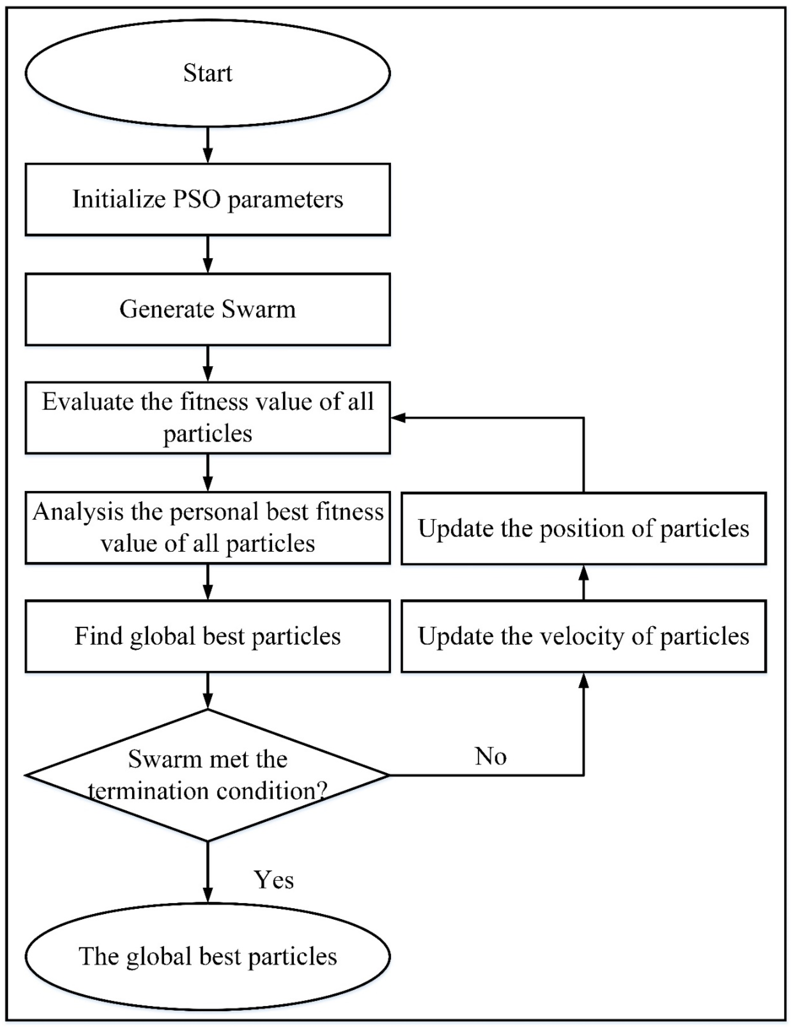
Figure 5.
Training performance of the CNN model.
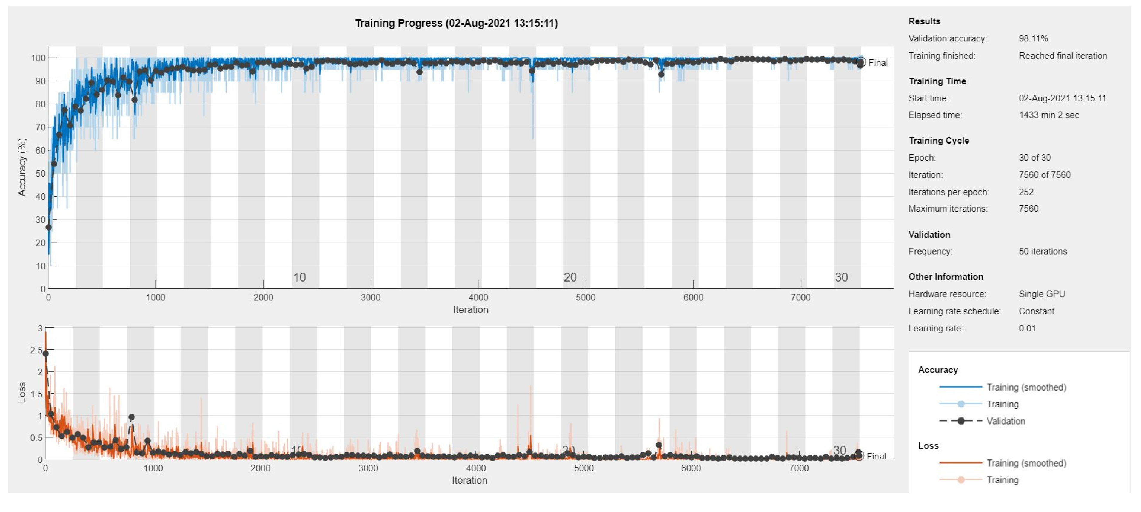
Figure 6.
Comparison of the training times of the SVM and KNN classifiers for different observations.
Figure 6.
Comparison of the training times of the SVM and KNN classifiers for different observations.
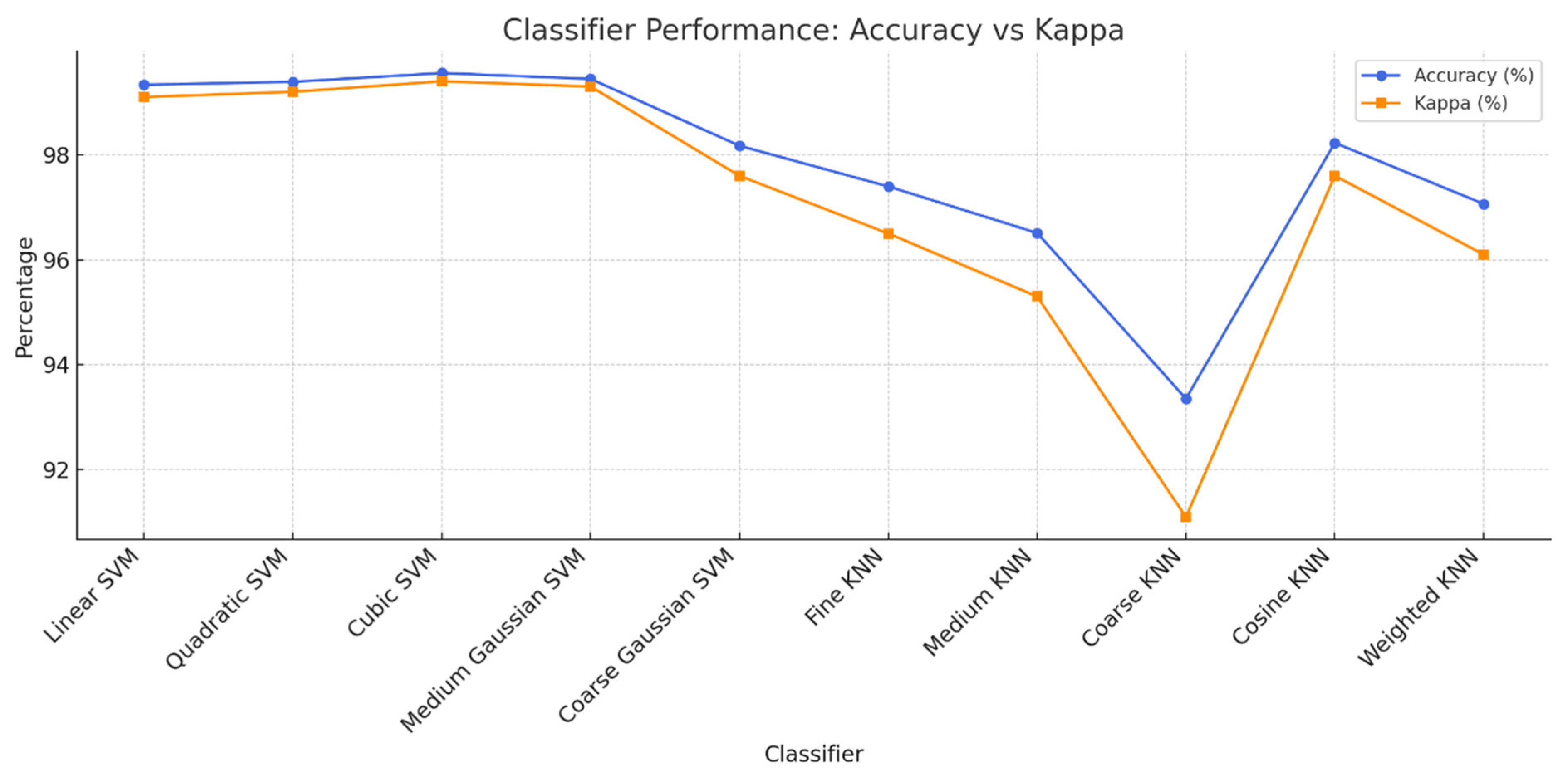
Figure 7.
Confusion matrix of the best result (750 features) of observation #4.
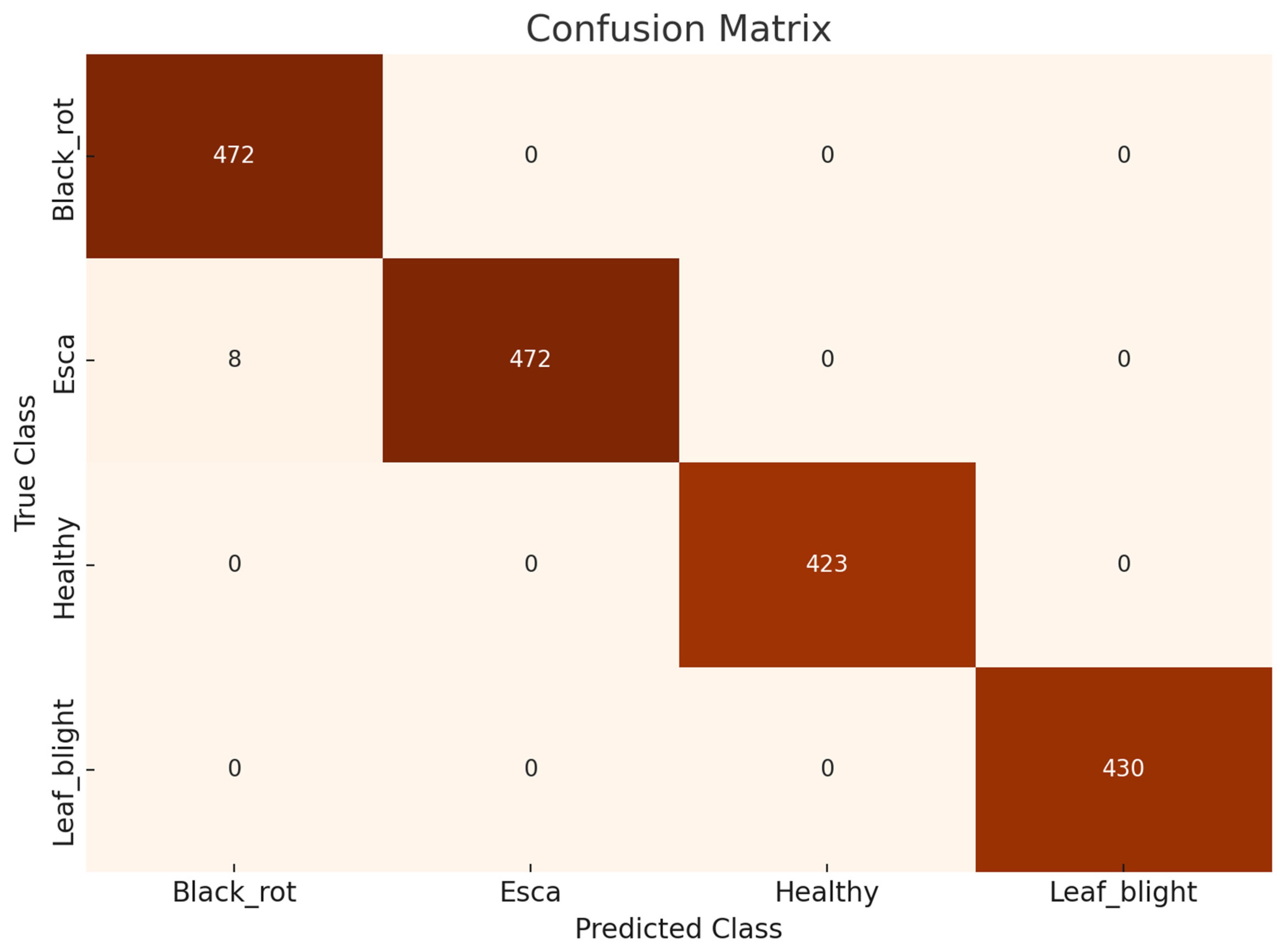
Figure 8.
ROC, AUC, and current classifier of the best result (750 features) of observation #6 for classes (i) Black_rot, (ii) Esca, (iii) healthy, and (iv) leafy blight class.
Figure 8.
ROC, AUC, and current classifier of the best result (750 features) of observation #6 for classes (i) Black_rot, (ii) Esca, (iii) healthy, and (iv) leafy blight class.
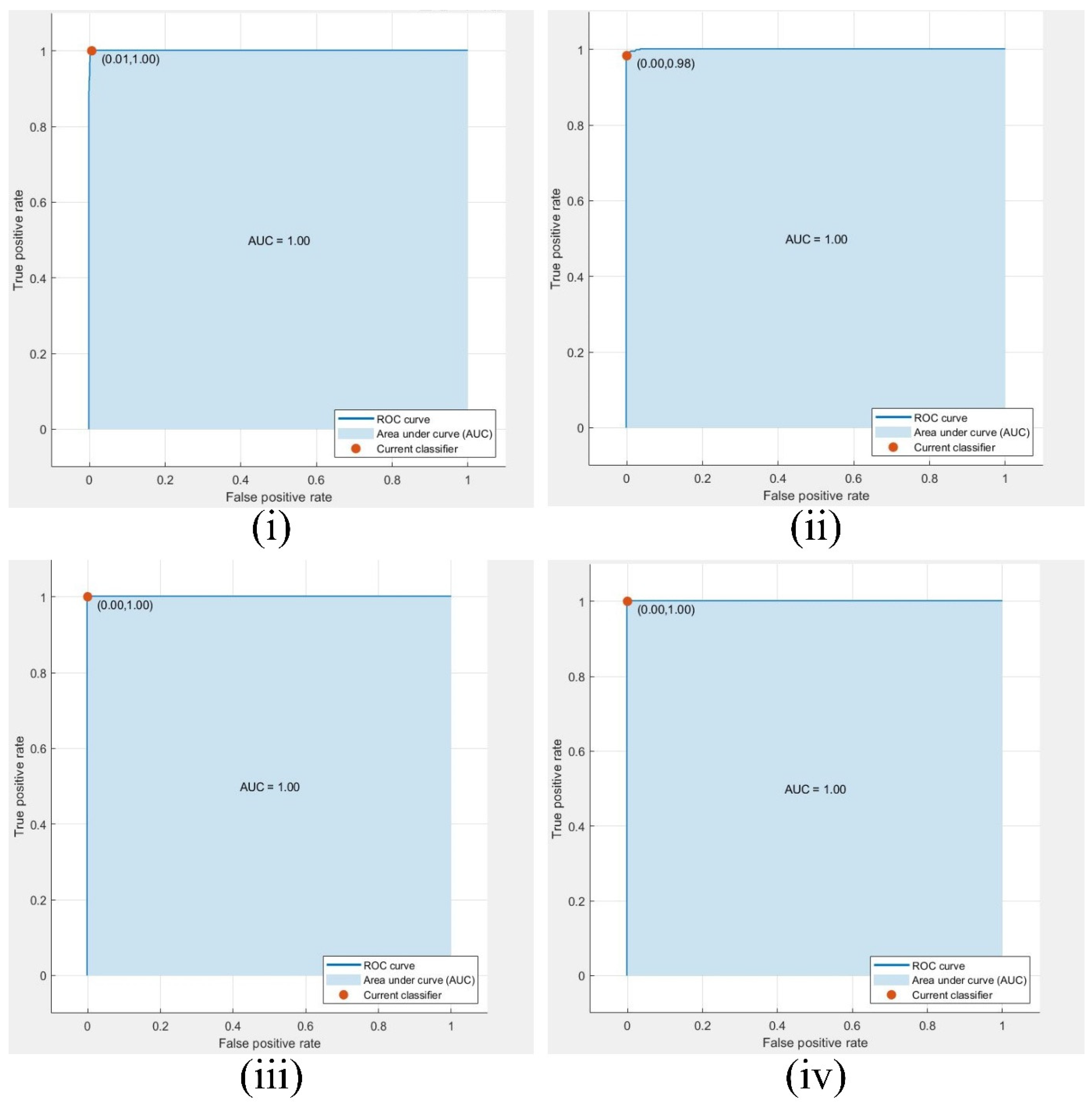
Figure 9.
Visualization of the outputs of the convolutional layers via the customized CNN network: (i) convL1, (ii) convL2, (iii) convL3, (iv) convL4, (v) convL5, (vi) convL6, (vii) convL7, (viii) convL8, (ix) convL14, (x) convL15, (xi) convL16, and (xiii) convL18.
Figure 9.
Visualization of the outputs of the convolutional layers via the customized CNN network: (i) convL1, (ii) convL2, (iii) convL3, (iv) convL4, (v) convL5, (vi) convL6, (vii) convL7, (viii) convL8, (ix) convL14, (x) convL15, (xi) convL16, and (xiii) convL18.
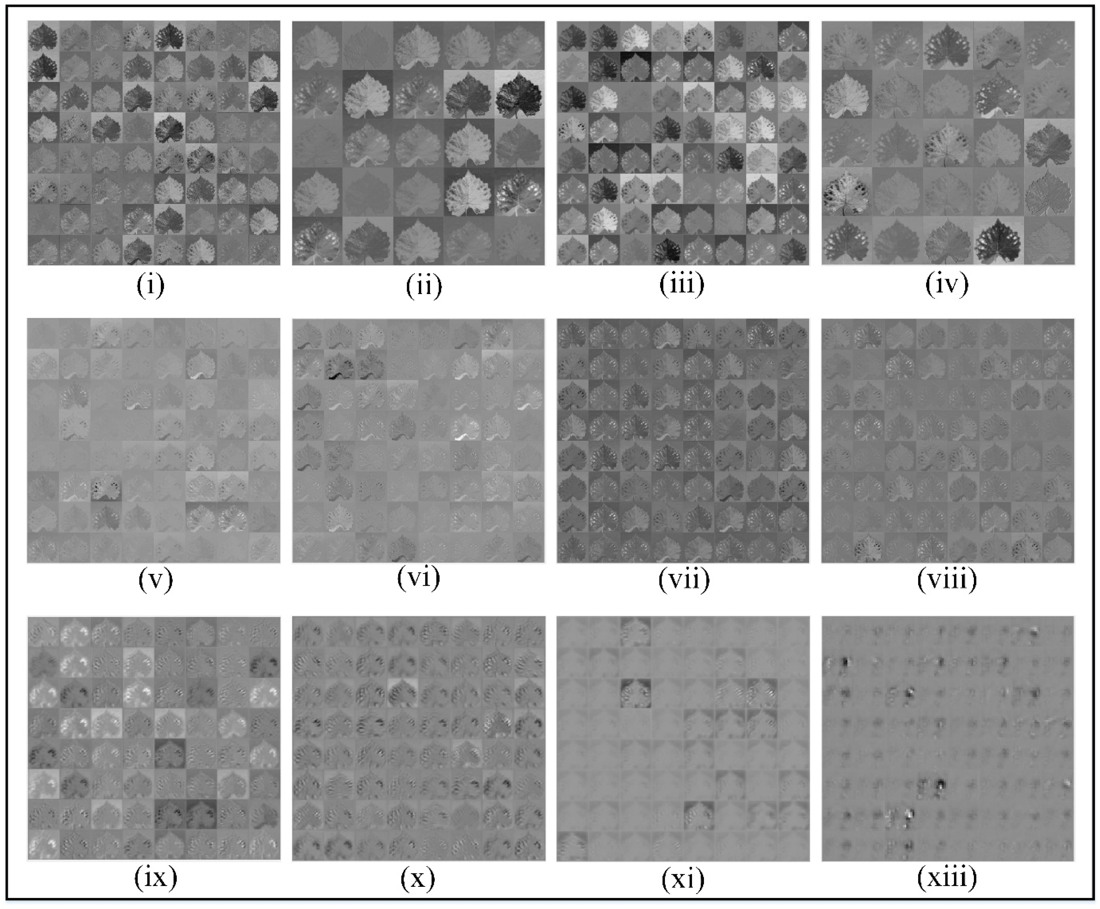
Figure 10.
Grad-CAM result of the customized CNN network on grape leaf images.
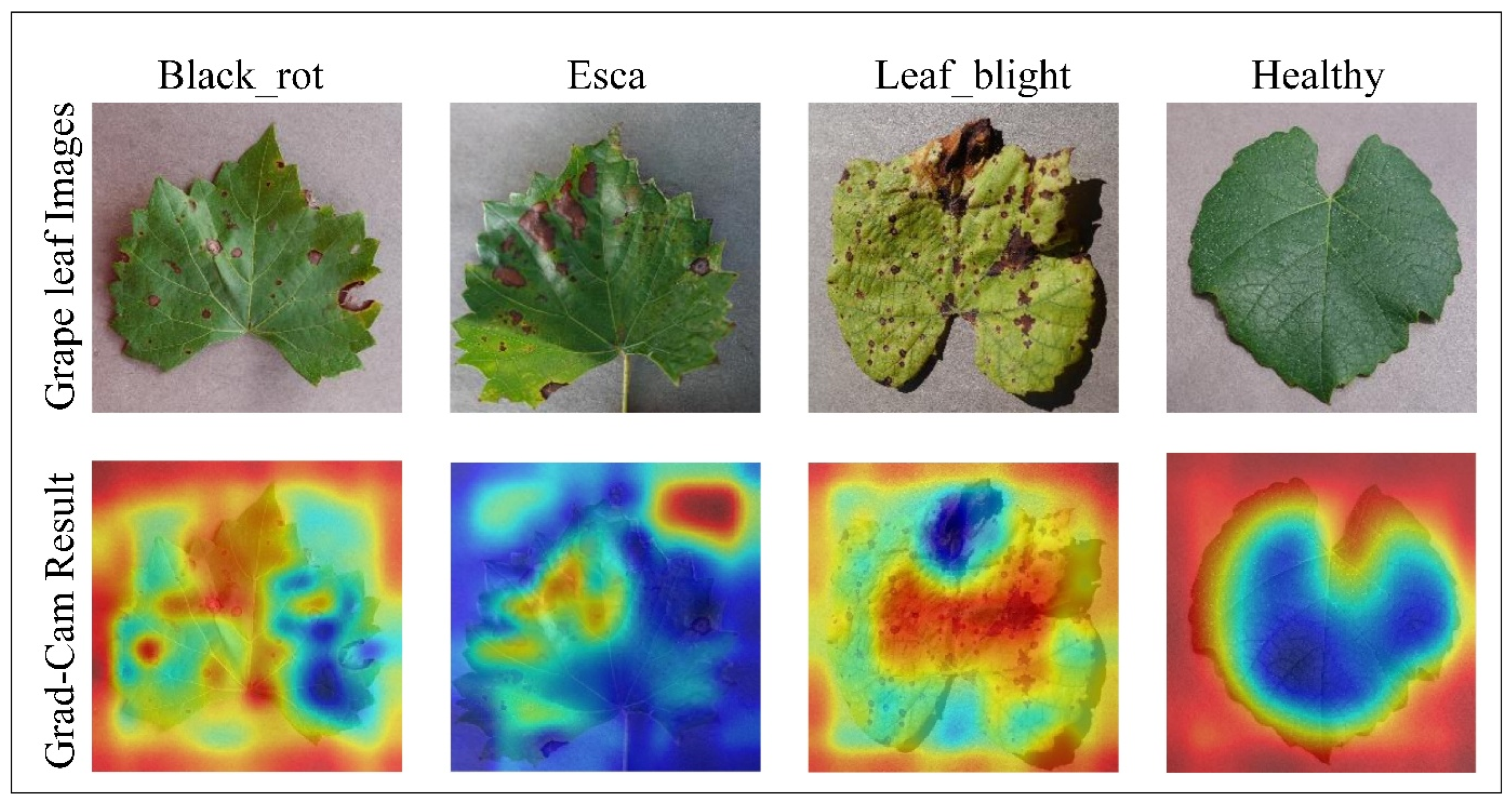
Table 1.
Number of images in the grape leaf dataset.
| Grape Leaf Diseases | ||
| Classes | Training | Testing |
| Black_rot | 1888 | 472 |
| Esca | 1920 | 480 |
| Leaf_blight | 1722 | 430 |
| Healthy | 1692 | 423 |
| Total | 7122 | 1805 |
Table 2.
Training parameters of B2-GraftingNet.
| Input Size | Learning Rate | Max Epochs | Mini Batch Size | Moment | Optimization |
| 227x227x3 | 0.01 | 30 | 20 | 0.9 | ADAM |
Table 3.
Number of features extracted via the B2-GraftingNet CNN model.
| Deep CNN Model | Feature Layer | Number of Extracted Features |
| B2-GraftingNet CNN model | ‘fc_1’ | 1,805 x 1000 |
Table 4.
Experimental results on different splits using optimized and non-optimized features.
| Observation # | Method | Number of features | Optimized result (%) |
| 1 | B2-GraftingNet features | 1805 x 1000 | 98.78 |
| 2 | B2-GraftingNet features →BPSO optimized features | 1805 x 100 | 98.615 |
| 3 | 1805 x 500 | 98.73 | |
| 4 | 1805 x 750 | 99.56 |
Table 5.
Classification results on several machine learning algorithms by 10-fold cross validation on BPSO optimized features from B2-GraftingNet.
Table 5.
Classification results on several machine learning algorithms by 10-fold cross validation on BPSO optimized features from B2-GraftingNet.
|
Test cases |
Classifiers |
Accuracy (%) |
Precision (%) |
Recall (%) |
Kappa |
Training Time (sec) |
| Test 1 | Linear SVM | 99.33 | 99.37 | 99.37 | 0.99 | 37.60 |
| Test 2 | Quadratic SVM | 99.39 | 99.43 | 99.43 | 0.99 | 38.84 |
| Test 3 | Cubic SVM | 99.56 | 99.58 | 99.58 | 0.99 | 42.15 |
| Test 4 | Medium Gaussian SVM |
99.45 | 99.47 | 99.48 | 0.99 | 50.88 |
| Test 5 | Coarse Gaussian SVM |
98.17 | 98.25 | 98.35 | 0.98 | 49.58 |
| Test 6 | Fine KNN | 97.40 | 97.50 | 97.55 | 0.96 | 51.37 |
| Test 7 | Medium KNN | 96.51 | 96.63 | 96.79 | 0.95 | 50.81 |
| Test 8 | Coarse KNN | 93.35 | 93.49 | 93.96 | 0.91 | 51.64 |
| Test 9 | Cosine KNN | 98.23 | 98.31 | 98.24 | 0.98 | 52.45 |
| Test 10 | Weighted KNN | 97.06 | 97.17 | 97.26 | 0.96 | 51.57 |
Disclaimer/Publisher’s Note: The statements, opinions and data contained in all publications are solely those of the individual author(s) and contributor(s) and not of MDPI and/or the editor(s). MDPI and/or the editor(s) disclaim responsibility for any injury to people or property resulting from any ideas, methods, instructions or products referred to in the content. |
© 2025 by the authors. Licensee MDPI, Basel, Switzerland. This article is an open access article distributed under the terms and conditions of the Creative Commons Attribution (CC BY) license (http://creativecommons.org/licenses/by/4.0/).
Copyright: This open access article is published under a Creative Commons CC BY 4.0 license, which permit the free download, distribution, and reuse, provided that the author and preprint are cited in any reuse.


