Submitted:
02 December 2025
Posted:
03 December 2025
You are already at the latest version
Abstract
Quantum mechanics introduces wave–particle duality as a postulate, yet the geometric origin of wave behavior has never been derived from first principles. Here we show that a finite quantum of action, ℏgeom, compactifies the classical action manifold into a periodic U(1) phase space. Physical observables then depend only on the modular action S mod 2πℏgeom, making interference a direct geometric necessity rather than an independent assumption. We formalize this as a theorem: any system possessing finite ℏgeom must exhibit wave interference, while the classical limit corresponds to decompactification ℏgeom→0. Chronon Field Theory (ChFT) provides the physical substrate for this geometry—its causal field Φμ carries quantized symplectic flux ∮ω=ℏgeom, thereby establishing Planck’s constant as a geometric invariant of causal alignment. This unified framework links modular action, quantization, and spacetime geometry, revealing the wave nature of matter as a necessary consequence of finite causal curvature. It further predicts quantized phase discontinuities in mesoscopic interferometry, offering a concrete path toward experimental validation.
Keywords:
quantum of action
; chronon field theory (chft)
; compact action manifold
; modular phase
; geometric quantization
; real–now–front (rnf)
; causal alignment
; emergent spacetime
; symplectic flux
; planck constant as geometric invariant
; wave–particle duality
; topological quantization
; quantum computation
1. Introduction
Quantum mechanics assigns transition amplitudes the form , making the phase of the action the operational quantity in every experimentally verified interference phenomenon. Yet neither the de Broglie matter-wave hypothesis [22] nor Feynman’s path-integral formulation [28] explains why physical observables depend only on the modular phase of S, rather than on its absolute value. In standard formulations this modular dependence is simply postulated.
The central observation of this work is that once the action possesses a finite geometric quantum , its domain is no longer the real line. A quantity identified only up to discrete increments of size takes values on the compact manifold
so that actions differing by become physically indistinguishable. On such a compact action manifold, interference is not an added axiom: it is a mathematical consequence. All observable amplitudes must be class functions on this compact space, and appears as its natural coordinate map. (See Appendix H for the geometric origin and decompactification behaviour of the action domain.)
We formulate this as a precise statement (Theorem 4.1):
If the action has a finite quantum , then all transition amplitudes are periodic in S with period , and wave-like interference necessarily follows.
To ground the finite action quantum physically, we draw on Chronon Field Theory (ChFT), a geometric framework in which the fundamental temporal field carries quantized symplectic twist. The twist two-form has integral
a topologically protected symplectic flux arising from stabilized chronon solitons (Appendix C). In this setting, Planck’s constant emerges not as an imposed quantization rule but as the minimal symplectic increment of the underlying causal medium. This aligns with geometric interpretations of quantum phase and holonomy in earlier work on geometric phase and symplectic topology [11,31].
A second foundational component is the Real–Now–Front (RNF), the dynamical “alignment front” that converts pre-geometric chronon microstates into the next geometric slice. The RNF operates as a compatibility- and energy-constrained reconstruction map (formal definition in Appendix B). Its selection of mutually compatible continuations provides the geometric basis for interference, decoherence, and the Born-weighted probability structure developed later in the paper (Appendix I; cf. decoherence analyses in [72]).
In this framework, entanglement emerges from global coherence in the internal chronon bundle, carried by vacuum gauge bridges linking the internal states of distant systems.
Taken together, these elements show that quantum interference—often regarded as an irreducible mystery—follows from a single geometric principle: a finite quantum of action equips the action manifold with compact topology, forcing phase periodicity and wave behavior.
The remainder of the paper develops this principle rigorously, connects it to the symplectic structure of ChFT, and explores its physical consequences.
Physical Intuition: Emergent Spacetime, the RNF, and the Geometry of Becoming
The underlying physical picture is not that the universe is filled with a background substance, but that the familiar structures of spacetime and matter arise from the dynamical alignment of a more primitive causal degree of freedom—the chronon field[41]. In this view, geometry, rods, clocks, and quantum interference emerge from how successive RNF slices are reconstructed. This resonates with broad themes in emergent spacetime research [9,51] but introduces two elements typically absent: (i) an operationally defined present, and (ii) a dynamical slice-to-slice reconstruction law.
A key point is that the Real–Now–Front (RNF) is not an extra structure inserted into spacetime; rather, the RNF slice is the three–dimensional world we inhabit at each instant. As the RNF advances, it brings the next moment of reality into existence. In the four–dimensional chronon picture, the 3D present is the infinitesimally thin boundary between an aligned geometric past and an unaligned pre–geometric reservoir that has not yet become actual.
This yields a concrete dynamical theory of Becoming, in contrast to the static block-universe picture criticized in the philosophical and foundations literature [55,56]. Instead of a timeless four-dimensional structure, new spacetime is continually generated as the RNF propagates.
A real underlying medium also provides a natural origin for an invariant causal speed. In ChFT, causal disturbances propagate as twist waves of the chronon field, and their velocity is fixed by the material stiffness of the medium, , rather than by kinematic postulate. Photons, massless neutrinos, and gravitational excitations all inherit this same propagation speed, making the universality of c a constitutive property of the medium itself. By contrast, a stage–only spacetime contains no mechanism that enforces a universal causal speed for different probes, even though experiments confirm such universality to extraordinary precision. This gap motivates the search for a dynamical spacetime framework grounded in a physical medium, where the invariance of c emerges from the microscopic structure rather than being imposed by fiat.
Crucially, the Co–moving Concealment Principle (CCP) ensures that the chronon medium’s preferred time direction does not manifest as observable Lorentz violation. The mechanism is similar in spirit to “emergent Lorentz symmetry” in analogue-gravity models [9], though implemented here through RNF reconstruction rather than quasi-particle kinematics.
The RNF framework also clarifies several quantum measurement puzzles. Each RNF slice must align chronon–pattern geometries that are compatible with apparatus constraints. Measurement-like selection therefore arises as RNF alignment choosing one compatibility basin during reconstruction, conceptually related to environment-induced selection in decoherence theory [72]. Nonlocal correlations—including delayed-choice and Bell-type phenomena—admit a natural geometric interpretation when the RNF is treated as a dynamical boundary where pre–geometric degrees of freedom become actual (Appendix M; cf. [10]).
The finite quantum of action enters this picture through the chronon medium’s quantized symplectic flux, , which compactifies the action manifold and enforces the universal phase factor . The compact–action theorem proved in this paper is therefore the geometric expression of the chronon medium’s minimal twist.
Importantly the RNF framework yields a concrete mechanism for entanglement: a global internal-bundle coherence structure—an emergent gauge bridge—that enforces nonlocal correlations without violating spacetime locality when the RNF andvances slice by slice.
A key phenomenological step in this work is the identification of the electron with the minimal chronon soliton. Its invariant quantum numbers endow it with a universal Compton wavelength and period [46], thereby providing intrinsic “rod” and “clock” scales that render the emergent Lorentzian metric operationally meaningful on each RNF slice.
Finally, we discuss the RNF implication for quantum computation and suggests new design principles that may lead to significant improvements.
Taken together, these features—emergent rods and clocks, an invariant causal speed, operational Lorentz symmetry, a dynamical present, and a geometric view of quantum measurement—position the compact–action/RNF framework as a coherent alternative to both block-universe models and standard quantum foundations.
Summary of contributions.
This work develops a single geometric framework in which spacetime, quantum behaviour, and particle phenomenology emerge from the dynamics of a chronon medium and its advancing Real–Now Front (RNF). Our main contributions are: (i) a compact–action formulation showing that quantum phases, the path–integral structure, and Schrödinger dynamics follow from RNF compatibility; (ii) a reconstruction-based account of measurement yielding the Born rule and macroscopic definiteness without external collapse postulates; (iii) a topological soliton sector in which twist defects realize fermionic degrees of freedom and curvature integrals determine particle masses and charges; and (iv) a horizon-alignment mechanism demonstrating exponential suppression of Hawking-like emission together with fully information-preserving black–hole evolution.
2. Foundations of Chronon Field Theory and the Temporal Coherence Principle
Chronon Field Theory (ChFT) supplies the physical substrate and mathematical structures from which the compact–action geometry developed in this paper arises[41,42]. Only the minimal ingredients required for the main results are summarized here. Detailed derivations and the full TCP formalism appear in the appendices: the configuration space and twist structure in Appendix A, the symplectic quantization mechanism in Appendix C, and the RNF reconstruction map in Appendix B.
ChFT is built on a single dynamical variable: a smooth, unit timelike covector
interpreted as the local orientation of physical time. No background metric is assumed microscopically; spacetime geometry appears only after sufficient alignment of , in line with broader ideas in emergent-gravity and analogue-gravity frameworks [9,51].
2.1. The Temporal Coherence Principle
The dynamics of are governed by the Temporal Coherence Principle (TCP):
The chronon field evolves so as to maximize local temporal alignment while suppressing incoherent twist and curvature.
The TCP is implemented by the action summarized in Appendix A, consisting of (i) a quadratic alignment term, (ii) an antisymmetric “twist’’ term measuring non-integrability (analogous to vorticity and spin-connection curvature [31]), (iii) a quartic stabilization term that prevents Derrick collapse and ensures finite–energy solitons [23,46], and (iv) a norm constraint enforcing .
Variation of this action yields the unified TCP field equation,
where the nonlinear term collects contributions from quartic gradients and enforces soliton stability.
In regions of low twist and curvature, these equations admit aligned solutions for which defines a coherent time direction and an effective Lorentzian metric emerges from the induced polarization frame. Thus the fundamental structure of ChFT is not a pre-existing metric but a dynamical causal field whose coherence properties generate geometry, echoing themes in hydrodynamic and analogue-emergent metrics [9,64].
2.2. Emergent Metric and Causal Structure
A spacetime metric appears only on sufficiently aligned regions, typically those already reconstructed by the RNF[41]. On such slices, determines parallel and transverse directions. The spatial projector
is therefore not a background structure but an artifact of successful alignment.
Linearizing the TCP equation around a coherent background yields, at long wavelengths, an effective Lorentzian metric
which governs the characteristics of small perturbations. Such emergent causal cones are standard in analogue-gravity systems and effective-field-theory treatments of Lorentz symmetry [43].
2.3. Gauge Sectors from Polarization Holonomy
The polarization directions transverse to form a naturally symplectic two–dimensional bundle. Parallel transport of polarization along aligned chronon trajectories induces a connection
where projects onto directions orthogonal to . Connections arising from internal frame transport are standard in geometric and gauge–theoretic formulations [31,48].
In the geometric limit (Appendix D), the curvature of this connection obeys equations with the same structural form as Yang–Mills dynamics, with the effective gauge group determined by the topology of the polarization fibers. The appearance of abelian and nonabelian sectors through bundle holonomy parallels familiar mechanisms in fiber–bundle gauge theory [13,48]. The abelian component yields electromagnetism; higher–rank sectors arise naturally from nontrivial holonomy of the polarization bundle.
Thus gauge interactions appear as emergent geometric effects of polarization twist, not as independent microscopic fields to be quantized[42].
2.4. Solitons, Finite Energy, and Symplectic Quantization
Chronon Field Theory admits localized, finite–energy excitations of the temporal field , which play the role of particle–like entities in the emergent spacetime. These configurations—chronon solitons—arise because the TCP action contains both quadratic alignment terms and quartic stabilizing terms. As shown in Appendix F, the quartic terms prevent Derrick collapse [23] and fix a preferred soliton core size
ensuring that finite-energy, finite-radius solutions exist and remain stable, as in standard topological–soliton models [46].
A central geometric feature of these solitons is the antisymmetric gradient of the causal field,
which encodes the twist of the polarization frame. Finite-energy boundary conditions compactify spatial infinity to , so the soliton defines a map whose degree is an integer, as in classic examples of topological charge [46,48]. This leads to a quantized symplectic flux,
derived in Appendix C. The integer n is the soliton’s topological charge, and the flux unit is a geometric invariant fixed by the chronon medium.
Thus solitons provide a natural candidate for the microscopic origin of a finite quantum of action.
2.5. Mass in Chronon Field Theory: Localization, Curvature, and Energy
In Chronon Field Theory (ChFT), “mass’’ is not a fundamental parameter but a derived property of how excitations of the chronon medium are supported. The theory distinguishes sharply between delocalized twist waves (intrinsically massless) and localized defects of the polarization bundle (intrinsically massive).
Three structural principles determine the ChFT notion of mass.
(1) Mass originates from the energy needed to localize an excitation.
To maintain a static, finite-size chronon defect, the polarization field must sustain both curvature and vorticity. The rest energy of a stationary soliton is the curvature functional
where the quadratic term measures alignment stiffness and the quartic Skyrme-like term provides stabilization against collapse. The soliton’s rest mass is the usual ratio
with the universal causal speed of twist waves. Thus mass in ChFT is the energy cost of localization: only excitations that require bounded curvature to remain finite carry mass.
(2) Linear twist waves are intrinsically massless.
Small-amplitude distortions of the chronon polarization frame satisfy the linear dispersion relation
admitting no static configuration and no curvature core. Such excitations neither localize nor store curvature energy, and so their rest mass vanishes. The photon (and any other pure transverse twist wave) is massless for this reason—not due to symmetry breaking, but because it is delocalized.
(3) Massive bosons correspond to localized polarization defects.
Any excitation of the polarization bundle that cannot propagate as a delocalized wave necessarily forms a localized core and therefore acquires mass through the same curvature functional as fermionic solitons. This yields a geometric reinterpretation of the electroweak sector:
- the photon is a pure twist wave () and massless;
- the correspond to charged () vector solitons with internal SU(2) curvature;
- the is a neutral () but topologically nontrivial SU(2) polarization soliton.
Their masses are the curvature energies of their respective localized cores. Thus the Higgs mass term of the Standard Model is re-interpreted in ChFT by the geometry and stability of localized polarization defects.
Our approach is in a manner analogous to other geometric derivations based on envariance [53].
(4) Boosted solitons reproduce the standard relativistic mass–energy relation.
A moving soliton corresponds to its localized curvature profile following the RNF advance. Because RNF reconstruction induces an emergent Lorentz metric with causal speed , the energy of a boosted soliton satisfies
with no additional postulates required. The usual relativistic mass–energy structure therefore follows from the covariant form of the TCP action and the RNF geometry.
Unified picture. In ChFT, mass is a localization energy: only excitations that require bounded curvature to remain finite acquire mass. Linear twist waves are massless; localized solitons (fermionic or bosonic) are massive; and boosted solitons follow standard relativistic mass–energy scaling. The electron, as discussed in Section 8, as the minimal soliton, is the simplest such massive defect.
Limitations and future work. A complete quantitative treatment of the bosonic soliton sector, including the detailed SU(2) polarization geometry and mass hierarchy, requires solving the full nonlinear TCP equations with internal gauge structure. This lies beyond the scope of the present work and will be developed in future studies.
2.6. Lorentz Invariance and the Co–Moving Concealment Principle
All observable excitations—solitons, photons, and polarization waves—are built from perturbations of itself. Thus they co-move with the chronon field, making any microscopic anisotropies dynamically unobservable. This yields the Co–Moving Concealment Principle (CCP):
Local observers constructed from chronon excitations can access only the emergent metric , not the underlying microstructure of .
Since all rods, clocks, and signals use the same chronon-based internal structure, they share the same limiting speed , guaranteeing operational Lorentz invariance. Short-scale deviations are washed out by co-moving concealment and remain experimentally invisible.
Thus Lorentz symmetry is not fundamental; it is the universal hydrodynamic limit of chronon coherence.
3. The Real–Now–Front as the Generator of Spacetime
Chronon Field Theory (ChFT) distinguishes two layers of structure: (i) a pre-geometric chronon medium with no metric, spatial relations, or propagating fields, and (ii) an aligned geometric domain in which spacetime, rods, clocks, solitons, and field excitations exist. The boundary between these regimes is the Real–Now–Front (RNF), a dynamical surface across which the chronon field first achieves alignment. The RNF is therefore the locus at which each new moment of physical reality is constructed.
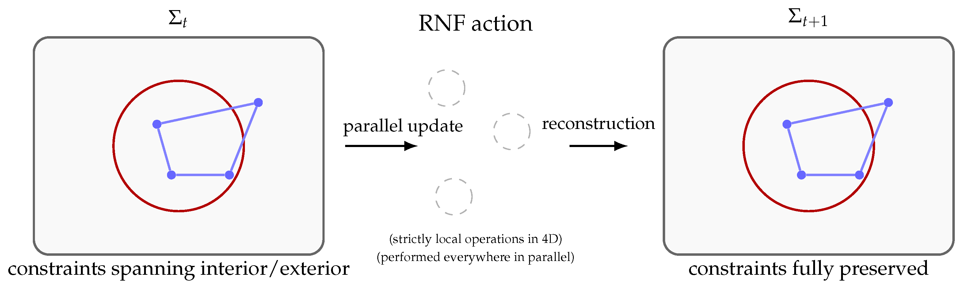
This section develops the RNF as a purely geometric reconstruction dynamics. The RNF converts pre-geometric microstates into an aligned metric slice, propagates matter and fields, and implements the selection of compatible pattern continuations. Its action is strictly local but applied everywhere in parallel, giving it the capacity to preserve global structures such as entanglement without requiring additional nonlocal mechanisms.
Detailed mathematical treatments are provided in Appendix A and Appendix B.
3.1. RNF Slices and the Structure of Becoming
Aligned configurations of the chronon field define an effective Lorentzian metric
so any hypersurface on which is aligned constitutes a geometric slice : a three-dimensional “present’’ endowed with spatial structure.
Ahead of lies the pre-geometric reservoir : an unrealized domain of chronon microstates with no metric, adjacency, or curvature. Behind the slice lies the frozen aligned past. The RNF is the infinitesimal boundary separating these domains:
The step is not evolution within a pre-existing spacetime. It is the construction of a new slice by local alignment of chronon microstates. The RNF thereby provides a fully dynamical account of Becoming: physical reality is continually generated slice by slice.
3.2. Local RNF reconstruction
For each point x on the next slice , the RNF applies a local reconstruction map
where is the portion of the pre-geometric reservoir that influences alignment at x.
Two structural principles determine :
- Local TCP minimization. Among all candidate microstates in , the RNF aligns the one that minimizes the local TCP energy density.
- Compatibility with the existing pattern. A microstate can be aligned at x only if it consistently extends the twist, polarization, and curvature data of the configuration on . Microstates that cannot be made compatible with by any local deformation are excluded.
These rules preserve structure entirely through local chronon dynamics, without any propagation of amplitudes or signals across the slice.
Simultaneous local reconstruction in 4D.
Because the RNF is a four-dimensional alignment boundary, it has no preferred reconstruction point. All maps act simultaneously across the advancing hypersurface, each using only its own local pre-geometric data. From within a 3D perspective this appears miraculous, but in 4D it is simply a parallel update rule acting on the entire RNF. The new geometric slice therefore emerges in a single step: locally reconstructed at every point, yet globally restoring all correlations “in one act.’’
3.3. Transport: How Patterns Move Across Slices
The reconstruction rules above determine which microstates may be aligned, but do not yet specify where each part of the pattern reappears. Motion and wave propagation arise from a transport map
obtained by minimizing the incremental TCP energy subject to compatibility with .
A pattern element at x is reconstructed at
where is the emergent shift vector. Transport and reconstruction are tightly coupled: the RNF aligns using the microstates near and the local compatibility inherited from via .
This yields:
- Soliton motion. A moving soliton is simply a localized curvature pattern translated by .
- Wave propagation. Linear twist excitations correspond to coherent regions of the shift vector, producing the usual dispersion .
- Constraint preservation. Global constraints—entanglement, holonomy, topological flux—are preserved because the entire constraint structure on is locally encoded (Section 6 and Appendix B) and reconstructed everywhere in parallel. is already a local representation of its own global constraint structure.
3.4. The RNF Entanglement Preservation Theorem
The local and parallel nature of RNF reconstruction gives rise to a powerful structural result:
Theorem 3.1
(RNF Entanglement Preservation). Let be an aligned slice containing a pattern with a global constraint structure Γ (such as entanglement relations, polarization holonomy, or topological flux). Let be the RNF reconstruction operator and the transport map. Then the RNF update preserves Γ exactly:
Sketch of proof. Global constraints are locally encoded in the structure of . RNF reconstruction is (i) strictly local, (ii) applied in parallel to all x, and (iii) restricted to microstates compatible with . Thus each constraint in is re-imposed at every point, yielding exact preservation even across horizons or disconnected regions of the emergent metric.
3.5. RNF as a Primitive Selection Mechanism
The RNF provides a physical mechanism for pattern persistence and pattern elimination without invoking collapse or decoherence postulates:
- Persistence. A soliton or field pattern persists only if every local RNF update admits compatible microstates; otherwise the pattern cannot be reconstructed.
- Environmental selection. Macroscopic apparatus patterns impose strong compatibility constraints: if an incoming pattern is compatible with only one macroscopic continuation, all others are excluded.
- Suppression of incompatible alternatives. If two candidate continuations have disjoint compatibility sets, the RNF cannot reconstruct both. Incompatible alternatives are eliminated geometrically.
These effects arise from the chronon dynamics and the TCP energy, not from Hilbert-space projection or observer-dependent collapse.
3.6. Summary
- The RNF is the dynamic boundary where pre-geometric chronon microstates are converted into coherent geometric structure.
- Local reconstruction and parallel application across the slice generate the entire next moment of spacetime in a single step.
- A transport map governs motion, wave propagation, and the location of reconstructed structures.
- Global constraints—including entanglement—are preserved automatically by the RNF Entanglement Preservation Theorem.
- Compatibility-driven reconstruction provides a geometric origin for pattern persistence, selection, and macroscopic definiteness.
As illustrated in Figure 2, the RNF is therefore the fundamental generative mechanism of ChFT: the process that builds spacetime, transports matter and fields, preserves global correlations, and selects the patterns that constitute physical reality.
4. Finite Quantum of Action: Compact Geometry and Wave Interference
A defining prediction of ChFT is the quantization of symplectic flux carried by any finite–energy chronon configuration. As shown in Appendix F, the twist two-form
satisfies the quantization condition
for every closed loop lying in an aligned region. The quartic term in the TCP action prevents continuous untwisting, forcing the flux to take discrete values. This is the same geometric mechanism underlying Dirac charge quantization [24] and the topological quantization of winding in nonlinear sigma models [46].
The existence of this minimal symplectic quantum has a profound and unavoidable consequence: the classical action becomes a compact variable. Configurations whose actions differ by cannot be distinguished by any geometric or dynamical process. The action thus lives on a manifold, and interference follows as the unique geometric law governing the composition of compact phases, as illustrated in Figure 3.
4.1. Compactification of the Action Manifold
In conventional mechanics the action S takes values in . In ChFT, a deformation that adds one unit of symplectic twist changes the action by
The two configurations differ by a topological sector of the chronon field, but all their geometric and dynamical properties coincide. They belong to the same compatibility class and cannot be distinguished by any physical measurement or any RNF reconstruction process.
Therefore the physical action takes values in the compact space
4.2. The Finite–Action Interference Theorem
The compact action manifold (7) leads to a unique interference law.
Theorem 4.1
(Finite Action Implies Interference). Let physically distinguishable histories be labeled by their action modulo . Then the detected intensity for two alternatives with actions must take the form
for apparatus-dependent constants .
Sketch.
The compact group has only the characters . Smoothness and normalization restrict physical weights to . Thus for two histories,
No other interference form is compatible with the compact geometry.
Interpretation.
Wave behaviour is a geometric necessity, not a postulate. Distinct trajectories correspond to points on , and their combined effect is determined by angle addition on a circle.
4.3. RNF Interpretation: Modular Action and Compatible Histories
The RNF does not use the absolute action S but only its compactified class . Actions that differ by an integer multiple of belong to the same compatibility set:
Thus the RNF propagates every geometrically compatible pattern continuation, each weighted by the phase (8). Summing these contributions gives the RNF analogue of the Feynman sum-over-histories:
Interference is therefore not a property of waves but the geometric consequence of compact action combined with RNF compatibility.
4.4. Double–Slit Interference as Compact Action Geometry
In the double–slit configuration the post-slit domain admits two compatible pattern classes and . They contribute phases and , so the RNF reconstructs the combined pattern
The detected intensity is
When which-path information is imposed, apparatus alignment constraints eliminate the overlap of compatibility sets, leaving only one admissible continuation. The interference term disappears automatically, without any collapse axiom, as demonstrated in Figure 4.
4.5. Summary
A finite quantum of action compactifies the action manifold into . This compact geometry forces:
- modular equivalence of actions differing by ,
- representation of trajectories by unitary characters,
- coherent sums of compatible RNF histories, and
- interference with period .
Wave behaviour is therefore the geometric manifestation of finite action, not an added axiom. Compact action makes interference inevitable, and the RNF supplies the local mechanism by which compatible modular histories combine.
5. Interference, Measurement, and Compatibility Collapse
With the compact action geometry established in Section 4, RNF reconstruction naturally produces two distinct behaviours:
1. Coherent combination of compatible modular histories (interference), and
2. Elimination of incompatible histories (collapse / measurement).
Both arise from a single mechanism: the RNF propagates all and only those chronon-pattern continuations whose microstates remain jointly compatible with the existing aligned pattern and any apparatus-imposed constraints. This section unifies interference and measurement under this single compatibility principle.
5.1. Modular Action and Compatible Pattern Continuations
Let be a chronon-pattern continuation from an initial point to a point x on the next RNF slice, with TCP action . Compactification of the action (Section 4) yields the equivalence relation
whenever the two patterns differ by one unit of symplectic twist. Patterns in the same modular class correspond to windings on the same action circle.
Let denote the pattern associated with . The RNF can propagate all of them precisely when their compatibility sets overlap:
When this overlap is nonempty, the RNF treats all such patterns as admissible continuations of the aligned slice.
Thus the familiar sum-over-histories expression,
is not a postulate but a compact description of RNF dynamics acting on modular action classes.
5.2. Interference From Multiple RNF-Allowed Histories
Suppose two pattern continuations and both satisfy (11). Their RNF-aligned contributions differ only by the modular action
Because the action lives on , the RNF cannot eliminate either continuation; both are propagated with relative phase .
The resulting field on the next slice is
and the intensity depends on the cosine of the modular phase difference, exactly as derived in the finite-action interference theorem (Section 4).
Wave-like behaviour is therefore not a separate ontological mode but the RNF’s geometric response to multiple simultaneously compatible pattern continuations on a compact action manifold.
5.3. Measurement as Compatibility Filtering
A measurement apparatus is a macroscopic chronon configuration with a highly rigid alignment structure and well-defined coherence domains. Let denote the incoming soliton pattern and the apparatus pattern. The RNF alignment map (Appendix B) is defined only on microstates belonging to the joint compatibility set
If several pattern continuations lie in this intersection, the RNF propagates all of them coherently (interference). If the intersection contains exactly one pattern class (up to modular phase), the RNF has no freedom: it must propagate that class. This is compatibility collapse. No additional collapse postulate is needed.
5.4. Decoherence and the Elimination of Incompatible Histories
Environmental interactions impose further alignment constraints that reduce the overlap of compatibility sets. For two competing patterns , coherence is possible only if
If environmental or apparatus structure drives this overlap to zero,
then the RNF cannot reconstruct both patterns on the same slice: one survives and the other becomes unreconstructible. This geometric elimination corresponds to decoherence-induced collapse in the standard formalism.
Thus decoherence is the process that shrinks compatibility overlap, while RNF compatibility provides the sharp condition that determines when interference must cease.
5.5. Born Weights and the Classical Limit
When many compatible histories contribute, the RNF-aligned field carries relative weights proportional to the stability volumes of their compatibility sets. In the continuum limit these volumes reproduce the standard Born weights, as shown in Appendix I (Theorem S1), where
In the macroscopic limit, apparatus constraints sharply localize these volumes, leaving exactly one dominant compatibility basin. The RNF then propagates a single classical trajectory, recovering definite outcomes and classical behaviour.
5.6. Summary
- Compact action forces patterns with modularly equivalent action to coexist as admissible continuations.
- RNF propagation combines all pattern continuations that remain jointly compatible with the existing aligned slice.
- Interference arises from RNF-aligned contributions of multiple compatible histories with relative modular phases.
- Measurement corresponds to additional apparatus constraints that restrict compatibility to a single pattern class.
- Decoherence occurs when environmental structure eliminates the overlap of compatibility sets.
- Collapse, definiteness, and the Born weights emerge from the geometry of compatibility, not from extra dynamical axioms.
Interference, measurement, and classical definiteness therefore share the same geometric origin: RNF reconstruction acting on chronon patterns with compact action and quantized symplectic structure.
6. Entanglement as Internal-Bundle Gauge Bridges
The RNF/ChFT framework offers a natural resolution to the longstanding question of how entangled systems separated by spacelike intervals can retain perfectly correlated behavior without violating emergent spacetime locality. The key insight is that the chronon field carries internal degrees of freedom—polarization, twist, modular-action phase, and gauge-like orientation—which are distinct from the external degrees of freedom associated with the emergent metric, soliton geometry, and classical field content. These internal DOFs form a gauge-like fiber bundle over each RNF slice , with local frames determined by the polarization and phase structure of the chronon medium.
A crucial empirical fact motivates this identification. Across more than eight decades of experimental quantum physics, all observed entanglement phenomena involve internal degrees of freedom—most famously spin and polarization in Bell tests [7,71], internal atomic levels in Rydberg and trapped-ion experiments [47], and flavor or mode indices in optical and particle settings. No experiment has ever demonstrated robust entanglement of external classical properties such as mass, spatial size, geometric shape, classical energy, classical frequency, or curvature. This sharp separation between “entangleable” and “non-entangleable” quantities—recognized since Schrödinger’s original analysis of non-separable internal-state correlations [59]—mirrors exactly the RNF distinction between internal and external chronon DOFs. The RNF framework explains this otherwise puzzling empirical dichotomy: only internal DOFs live in a global bundle structure that can support the nonlocal coherence patterns characteristic of entanglement.
In this section we show that quantum entanglement corresponds to a global constraint pattern in the internal chronon bundle, which we call an internal-bundle gauge bridge (or simply a gauge bridge). Unlike solitons, which are topologically protected excitations in the external configuration of the chronon field, gauge bridges are non-topological, global defects in the internal bundle geometry. They carry no energy, produce no curvature, and do not modify the external metric structure. However, they impose strict constraints on the RNF reconstruction of internal chronon DOFs across , thereby enforcing the correlations characteristic of entangled states.
6.1. External vs. Internal Degrees of Freedom
Each chronon carries two classes of DOFs:
- External DOFs: the alignment and curvature data that give rise to the emergent Lorentzian metric, soliton cores, and macroscopic fields. These DOFs obey emergent locality and are governed by the coherence of the temporal field . No experiment has ever observed entanglement of purely external DOFs such as mass, size, classical energy, position shape, or curvature, reflecting the fact that external DOFs cannot support nonlocal compatibility constraints in RNF.
- Internal DOFs: the polarization, twist, and compact-action phase associated with each chronon. These form a local gauge-like fiber (typically an or -type internal space) above each point of . They are invisible to classical observables but essential for modular-action interference and RNF compatibility reconstruction. All experimentally confirmed instances of entanglement occur exclusively within this class of DOFs.
The distinction parallels—but is more physically grounded than—the separation between base-space geometry and internal gauge spaces in Yang–Mills theory. In RNF/ChFT, however, these internal bundle structures determine not only the long-wavelength gauge interactions but also the global coherence patterns responsible for quantum entanglement.
6.2. Definition of a Gauge Bridge
Consider two solitons A and B supported on disjoint regions of . We define a gauge bridge between A and B as a global constraint on the internal chronon bundle satisfying:
- The bridge imposes a non-factorizable relation between the internal DOFs of A and B, matching the empirical fact that only internal DOFs are observed to entangle.
- The constraint is encoded in the internal DOFs of the vacuum chronons spanning the region between A and B.
- No topological charge protects the bridge; it is stabilized purely by internal-bundle coherence.
- The constraint is preserved by the RNF update if and only if the local compatibility sets of the internal DOFs remain jointly consistent.
A spin singlet provides a canonical example. On the internal-bundle polarization fields encode the antisymmetric constraint
where are the internal polarization vectors in the fiber above the soliton cores. This relation is implemented not by a physical “string” or flux tube connecting the solitons, but by a synchronized internal-bundle polarization pattern extending throughout the vacuum region. Although energetically trivial, the pattern places global restrictions on allowed chronon microstates and therefore on RNF-compatible reconstruction paths.
6.3. Preservation and Destruction of Gauge Bridges
Gauge bridges are inherently non-topological. Unlike solitons, whose topological winding protects their identity, gauge bridges rely entirely on global coherence of the internal chronon bundle. As a result, they are fragile: any local interaction that enforces an incompatible alignment of internal DOFs destroys the global pattern.
Formally, let denote the internal-bundle constraint defining the gauge bridge. The RNF update from to preserves if and only if the local compatibility sets at every point admit a continuation that satisfies the global constraint. A measurement, scattering event, or environmental coupling introduces new local alignment constraints that may render the global pattern incompatible. In this case, the RNF update cannot reconstruct , and the gauge bridge collapses in a single step.
This mechanism provides a physically concrete account of decoherence: entanglement decays when environmental interactions disrupt the coherent internal-bundle polarization pattern of the vacuum, eliminating the conditions required for RNF to reconstruct the global constraint.
6.4. Entanglement as a Gauge-Theoretic Phenomenon
Gauge bridges reveal entanglement as a fundamentally gauge-theoretic phenomenon. The nonlocal correlations originate not from the geometry of emergent spacetime but from the global coherence of the internal DOFs of the chronon field. The RNF propagates these correlations because the internal bundle over carries a global constraint pattern that restricts how internal DOFs can be reconstructed across the slice. When the pattern is intact, entanglement persists; when the pattern is disrupted, the RNF must select a locally compatible continuation and the bridge disappears.
Thus, entanglement is neither mysterious nor fundamentally spacetime nonlocal: it is a global internal-bundle constraint enforced by RNF reconstruction, closely analogous to parallel-transport constraints and holonomy structures in gauge theory but realized in a spacetime-emergent medium. As illustrated in Figure 5, the empirical restriction of entanglement to internal DOFs is therefore not accidental but reflects the fundamental structure of the chronon field: only internal DOFs inhabit the bundle geometry capable of supporting gauge bridges, while external DOFs remain strictly local and classically reconstructible.
6.5. Vacuum Capacity of the Internal Bundle
Mathematically, the distinction between external and internal DOFs can be encoded as a splitting of the chronon configuration space on each RNF slice . Let
denote, respectively, the spaces of external and internal field configurations, where is the internal (gauge-like) bundle and its space of smooth sections. A full RNF configuration can then be represented as a pair
The vacuum external sector is defined by fixing a background metric and soliton content,
so that all remaining dynamical freedom resides in the internal configuration . Since has fiber dimension at each , the space is an infinite-dimensional function space even when is held fixed. In particular, the subset corresponding to a fixed finite collection of solitons,
still forms an infinite-dimensional manifold of sections that agree with the required internal data near A and B but remain unconstrained on the surrounding vacuum region.
A gauge bridge between A and B can then be represented as a nontrivial constraint submanifold
defined, for example, by a functional relation
that links the internal DOFs of A and B via their continuation through the vacuum. Because is infinite-dimensional while is specified by finitely many global constraints, the vacuum internal bundle has ample capacity to support such global patterns without exhausting its available DOFs.
In this sense, the aligned vacuum possesses a large reservoir of internal-bundle degrees of freedom: fixing the external configuration and a finite set of solitons places only mild constraints on , leaving an infinite-dimensional family of internal configurations available to realize gauge bridges. Entanglement corresponds precisely to the RNF selection of configurations within such constraint manifolds .
Consequently, the RNF/ChFT framework predicts the complete absence of gravitational entanglement, since the external metric sector cannot support internal-bundle gauge bridges.
7. Beyond Schrödinger Dynamics: RNF Quantum Mechanics
A viable reformulation of quantum theory must recover standard quantum mechanics in the experimentally tested regime while offering deeper explanatory structure. In the RNF/Chronon Field Theory (ChFT) framework, this recovery is not imposed but follows from two geometric facts:
(1) a finite quantum of action compactifies the action manifold and enforces phases of the form , the same structure that underlies the Feynman path-integral phase rule [28];
(2) RNF reconstruction restricts propagation to families of chronon configurations whose actions lie in the same modular class, paralleling the topological equivalence classes in action-based formulations [57].
Measurement, entanglement, and macroscopic definiteness arise from the geometry of compatibility basins and the structure of the pre-geometric domain. Where tested, the RNF predictions agree with standard quantum mechanics; where standard QM provides no mechanism, the RNF supplies geometric explanations.
7.1. Compact Action and the Quantum Phase
Section 4 and Appendix C establish that a finite symplectic flux quantum carried by chronon solitons identifies action values modulo , as in topologically restricted path integrals [57]. The only continuous characters on the compact action manifold are
precisely the quantum phase structure found in geometric formulations of interference [11]. Thus the phase rule of quantum mechanics arises naturally from compact action.
7.2. RNF-Compatible Families and the Path Integral
The RNF advances by reconstructing the chronon field in a thin shell ahead of the aligned region. Only pattern geometries whose actions fall within the same modular class remain RNF-compatible:
The reconstructed field at is therefore
matching the Feynman sum-over-histories restricted to RNF-admissible trajectories [28]. The RNF composition law produces the usual propagator convolution.
7.3. Recovery of the Schrödinger Equation and RNF Corrections
Appendix J shows that, for slowly varying potentials and long-wavelength solitons, the RNF composition law reduces to Schrödinger evolution:
The RNF framework predicts small corrections arising from:
- nonlocality of RNF reconstruction on soliton-core scales;
- quartic TCP terms modifying dispersion;
- higher-order curvature of the compact action manifold.
All corrections are suppressed by the alignment scale , leaving standard QM an excellent low-energy limit.
7.4. Wave Function as a Twist–Phase Field on
Once the RNF kernel is shown to reduce to the Schrödinger equation (Appendix J), it is natural to ask: what is the wave function in this framework?
At a fixed RNF time t, the slice is a three-dimensional space on which the chronon field is aligned. The wave function
may still be viewed as a complex scalar field on , but its components acquire a geometric meaning:
- is the density of RNF-compatible microcontinuations through , i.e. the local alignment volume for the next slice.
- is the compactified action phase accumulated by RNF histories ending at .
Geometrically, one can think of each point as carrying two pieces of structure: (i) a local chronon polarization/twist direction in the transverse bundle, and (ii) a phase angle on the action circle. Figure 6 represents this as a lattice of points, each decorated by a “twist arrow” (underlying chronon orientation) and a “phase arrow” (action phase). The overall density and intensity of the arrows in a region encode , while the phase arrows encode .
7.5. Measurement as Compatibility Selection and the Born Rule
Measurement devices impose rigid boundary conditions on the RNF, defining discrete compatibility basins for possible outcomes. Let denote the RNF-compatible families associated with outcome i. Appendix I shows that the reconstruction probability is
which reduces under general regularity assumptions to the Born rule , the standard quantum prescription [15]. Probability weights therefore arise from geometric compatibility, not axiomatic postulates.
Collapse corresponds to incompatibility: if , only one basin can be propagated by the RNF.
7.6. Resolution of Standard Quantum Paradoxes
Wave–particle duality and the unified pattern ontology.
In the RNF picture a chronon soliton never ceases to be reconstructed: at each advance the front regenerates a coherent pattern that preserves all compatible twist and curvature constraints. As long as a family of continuations remains mutually compatible, all of its members persist slice by slice; none are eliminated until a macroscopic apparatus forces the RNF dynamics to select a single compatibility basin. In this sense, the standard intuition of wave–particle duality remains valid but gains a deeper foundation: the “particle” is the persistent soliton reconstructed on each slice, while the “wave” is the structured family of all RNF–compatible continuations carrying action phase relations.
The result is a unified ontology: everything that appears as a “wave” or a “particle’’ is, in fact, a chronon pattern undergoing RNF reconstruction. The supposed duality dissolves; only patterns and their compatibility relations remain fundamental.
Collapse and decoherence.
Collapse is geometric incompatibility (Section 5). Decoherence corresponds to environmental constraints reducing overlap of compatibility sets.
Uncertainty.
Minimal symplectic flux implies that a chronon soliton cannot simultaneously maintain sharply localized twist and perfectly smooth polarization. Localizing the twist within a region of size forces large gradients in the polarization frame, which contribute a curvature energy bounded below by the fixed action quantum . Conversely, reducing polarization gradients to improve smoothness necessarily spreads the twist over a larger region. The product of spatial width and phase–gradient width therefore obeys a geometric lower bound of order , so the familiar uncertainty relation arises not from operator algebra but from the intrinsic twist–smoothness tradeoff enforced by the chronon medium’s finite symplectic flux.
Double-slit and delayed choice.
Interference arises whenever more than one compatibility family survives; which-path constraints remove overlap. Delayed-choice experiments modify the constraints on the slice where reconstruction occurs but do not retroactively change past geometry.
Macroscopic definiteness (Schrödinger’s cat resolved).
The real paradox in Schrödinger’s cat is not that “alive’’ and “dead’’ are incompatible macroscopic states—everyone agrees they are. The issue is that in standard quantum mechanics the composite wavefunction must evolve unitarily until an external measurement occurs. Nothing inside the formalism selects one macroscopic alternative before the box is opened, so the theory predicts an evolving superposition of an alive–cat configuration and a dead–cat configuration with no physical mechanism for when or how one branch becomes real. In the RNF framework, the advancing front must realize a single macroscopic compatibility basin on each slice. Rigid basins such as “alive’’ or “dead’’ are mutually exclusive and only one can be reconstructed. Thus macroscopic definiteness is enforced during RNF alignment, not by external observers.
7.7. Entanglement as a Joint Internal-Bundle Constraint Preserved by RNF Reconstruction
In ChFT, quantum entanglement is not a mysterious nonlocal influence but a single global constraint in the internal chronon bundle encoded directly in the aligned pattern on each RNF slice. An entangled configuration is a pattern whose allowed continuations are restricted by an internal-bundle relation such as
for a spin singlet. This constraint is not carried by spacetime geometry or external soliton structure; rather, it is encoded in the coherent polarization and phase alignment of the vacuum chronons forming an internal-bundle gauge bridge linking the two systems.
When the RNF advances to , reconstruction proceeds in parallel at all points with no preferred update location. Each point samples the pre-geometric reservoir only from those microstates consistent with the full internal-bundle pattern on . Because the gauge-bridge constraint is represented throughout the vacuum region connecting A and B, RNF reconstruction automatically re-imposes the same internal relation on the next slice. No information or influence needs to be “transmitted” across the emergent metric; the global constraint is simply part of the local compatibility structure used in reconstruction.
Spatial separation does not weaken or modify the constraint because distance, causality, and geometric locality are products of the same RNF reconstruction process that also enforces the internal-bundle constraint. During each RNF update, every point of applies the same local compatibility rule in parallel, with no preferred update location: the external positions of A and B and the internal-bundle relation linking them are all fixed through this uniform, slice-wide alignment step. This yields the familiar quantum correlations—including those violating Bell inequalities [10]—without any nonlocal signaling.
Figure 7 illustrates this mechanism.
7.8. Horizon Alignment, Hawking Suppression, and Stable Micro Black Holes
In semiclassical gravity, Hawking radiation arises from trans-horizon mode mixing of quantum fields near the horizon [34,35,63]. This calculation assumes a fluctuating quantum vacuum with arbitrarily short-wavelength degrees of freedom and a horizon that efficiently mixes modes across an exponentially stretched coordinate transformation.
In the RNF/ChFT framework none of these assumptions hold. The quantum vacuum is a fully aligned chronon configuration rather than a sea of fluctuating field modes; excitations are twist and curvature waves with a built-in ultraviolet cutoff . The horizon therefore acts not as a particle amplifier but as a one-sided geometric boundary: geometric signals cannot propagate outward from inside, but RNF reconstruction still uses the global pre-geometric constraint structure when generating each new slice.
Attempting to extend curvature-alignment waves across the near-horizon layer requires a TCP misalignment cost. As shown in Appendix L, this cost scales at least as
leading to an exponentially small upper bound on the reconstruction probability,
with an order-unity stiffness parameter. Multiplying this suppression by the dimensional leakage scale yields an emission upper bound that is many orders of magnitude smaller than the Hawking rate for any macroscopic horizon.
For astrophysical black holes the ratio is so large that the RNF emission bound is effectively zero, rendering such objects non-radiative in practice. For horizon radii near the alignment scale, , the bound weakens and long-lived compact objects become possible. This provides a natural RNF mechanism for stable micro black holes and chronon-core condensates, with potential implications for dark-matter phenomenology.
Electromagnetic silence of black holes. Both in standard GR and in RNF/ChFT a neutral black hole emits no electromagnetic radiation: classically the horizon hides all internal gauge structure, and in ChFT the interior chronon core is a maximally aligned phase in which all gauge and matter degrees of freedom are frozen. Thus EM emission is identically zero in both pictures; the only possible radiative channel is the gravitational (or curvature–alignment) sector. The key difference is therefore not electromagnetic behaviour but the near total suppression of Hawking-like graviton emission in the RNF framework.
Comparison with ordinary thermal emission. A proton-scale black hole has radius . In standard Hawking theory it would radiate violently, , owing to its enormous temperature .
For intuition, a cold body of the same geometric size placed in a background would emit only .
In RNF/ChFT the emission rate acquires an exponential suppression ; with this yields
far below even the scale of ordinary cold-body radiation. Thus a proton-scale RNF black hole would be colder than any naturally occurring object, with emission suppressed beyond any observational reach.
7.9. Entanglement, Horizons, and Information Preservation in RNF/ChFT
The RNF reconstruction rule provides a simple and structurally clean resolution of the black–hole information problem. In ChFT, evolution does not occur by geometric propagation of fields through an existing spacetime. Instead, the RNF generates each new slice by local, parallel copying of the chronon pattern encoded on , selecting only those microstates compatible with that pattern. No external memory, nonlocal mediator, or additional structure is required: the pattern on the slice itself already embeds all the constraints and correlations needed for reconstruction.
Horizons limit geometric signals, not RNF reconstruction.
A black–hole horizon prevents causal influences in the emergent metric, but it does not impede the RNF. Reconstruction does not rely on communication across the slice; it occurs locally and simultaneously at all points. Because the constraint network—including entanglement relations, holonomy, and topological flux—is already encoded on , the RNF simply reproduces that pattern when building . Interior and exterior constraints are treated on equal footing. Thus, entanglement across a horizon is automatically preserved without any need for geometric transport.
The black–hole interior is continuously rebuilt.
The interior never becomes an isolated or forgotten region. Every RNF step reconstructs the entire chronon pattern, including the interior, using the same local copying rule as everywhere else. The geometric horizon appears only after alignment, as a feature of the emergent metric, and does not affect the underlying pattern that the RNF uses as its input.
Information is never lost.
All correlations—including those that appear nonlocal in the emergent geometry—are preserved because they are encoded in the aligned pattern of each slice and re-imposed by RNF reconstruction. Since Hawking-type emission is exponentially suppressed in ChFT (see Sec. Appendix L), no thermal flux of mixed states is produced. The evolution remains fully deterministic, slice by slice, and no information is lost. The firewall paradox [5] arises only if one assumes that entanglement must be transferred geometrically across the horizon, an assumption that ChFT does not require.
Consequences.
This framework avoids all of the standard semiclassical difficulties: there are no firewalls, remnants, nonunitary processes, or exotic entanglement-transfer mechanisms. An entangled pair remains entangled even when one partner crosses the horizon, because the entanglement is a constraint built into the pattern and replicated on each new slice. RNF/ChFT therefore provides a simple, robust, and locality-preserving mechanism through which black holes remain fully information preserving.
In summary: RNF reconstruction preserves the entire constraint network across slices, reconstructing both exterior and interior regions simultaneously. The horizon restricts only geometric propagation, not the RNF itself. As a result, black holes do not lose information in ChFT.
Figure 8.
RNF reconstruction across a black–hole horizon. Left: On slice , the constraint network—including entanglement links and topological flux—spans both interior and exterior regions. Middle: As the RNF advances, reconstruction proceeds through strictly local alignment rules applied simultaneously at all points. No geometric communication or nonlocal mechanism is required. Right: On , the entire pattern is faithfully reconstructed, including all constraints that cross the geometric horizon. Thus information is preserved slice by slice despite geometric causal barriers.
8. Phenomenology: The Electron as the Minimal Chronon Soliton
The compact–action/RNF framework by itself does not specify which excitations of the chronon medium correspond to the known particles. Once the soliton sector of Chronon Field Theory (CFT) is included, a highly constraining identification emerges: the electron is the minimal, topologically complete chronon soliton. This section summarizes why this identification is essentially forced by the theory and how it is consistent with existing experimental bounds.
8.1. Theoretical Motivation
In CFT the chronon vorticity defines a conserved topological flux. Finite–energy configurations are labeled by an integer winding number n, and the quartic TCP terms stabilize localized solitons carrying this flux. The minimal nontrivial configuration has and constitutes a single, topologically complete chronon vortex. Higher- solitons necessarily carry larger emergent charge.
Because the emergent Abelian gauge sector assigns electric charge directly to the winding number, a configuration with n units of flux carries electric charge n in electromagnetic units. Thus a particle with unit electric charge must correspond to the minimal soliton; composites would carry or require an internal pair of opposite-charge solitons.
Spin supplies an independent constraint. The chronon polarization bundle has a nontrivial double-cover structure, so that a rotation acts as the nontrivial element of the cover. A single vortex coupled to this bundle acquires spin in the emergent low-energy description. Multisoliton composites would generically yield higher or mixed spin representations and could not robustly produce an exactly -spin pointlike excitation with no multiplet structure.
Thus:
- minimal topological flux (),
- unit electric charge,
- and the double-cover spin structure,
collectively force the identification of the electron with the single minimal chronon soliton. The soliton core radius is naturally of order the chronon scale and therefore Planck-like, consistent with the electron’s apparent pointlikeness at all accessible energies.
8.2. Consistency with Electron Size and Compositeness Bounds
A soliton solution sounds “extended,” yet high-energy scattering shows the electron to be pointlike down to extremely short distances. In the chronon picture this is explained by the hierarchy
where is the soliton core, the shortest experimentally probed distance in scattering, and the Compton wavelength.
Current collider bounds on electron compositeness [4,49] require any internal structure to lie above the multi-TeV scale, consistent with the chronon prediction that is many orders of magnitude larger.
In addition:
- Known scattering experiments probe and are sensitive only to the integrated topological flux, so the electron appears strictly pointlike.
- The agreement between theory and experiment for the electron anomalous magnetic moment [6] implies that any composite effects must be suppressed by , again consistent with a Planck-like soliton core and extremely high compositeness scale.
Thus all current “pointlike electron’’ data constrain the chronon scale but remain fully compatible with the minimal-soliton identification.
8.3. Electron Quantum Numbers as Soliton Invariants
In ChFT the electron corresponds to the minimal finite-energy soliton carrying one unit of the fundamental symplectic flux. Its observed quantum numbers arise as geometric invariants:
Electric charge.
The Abelian polarization connection yields a gauge potential , and the electric charge is
The minimal soliton corresponds to .
Spin.
Spin arises from the holonomy of the polarization frame around a loop linking the core:
Thus the soliton transforms as a doublet and carries .
Mass.
As explained in Section 2.5, the soliton mass is the rest energy of the static chronon configuration. For a stationary solution the TCP energy functional reduces to the curvature–alignment integral
which contains the quadratic (alignment) and quartic (stability) curvature invariants of the chronon field. The second term is the Skyrme-like stabilizer required by Derrick scaling [23].
The electron mass is then defined by the usual rest–energy relation
Because depends only on the stiffness parameters and the fundamental alignment length , matching the observed value of fixes a single dimensionful combination of these parameters—equivalently, the effective curvature scale of the soliton core. Thus the electron’s mass, charge, and spin emerge together as geometric invariants of the soliton, endowing it with its operational role as the metrological rod and clock that defines the emergent Lorentz metric on each RNF slice. A schematic illustration is shown in Figure 9.
8.4. Existing Experimental Constraints
Three empirical domains already constrain the minimal-soliton picture:
Scattering and compositeness.
Anomalous magnetic moment.
The precision of the electron [6] implies that any soliton-induced correction must be minminuscule. This is naturally satisfied since chronon corrections scale as with .
Absence of excited electrons.
8.5. Possible Future Tests
Although direct access to the chronon scale is infeasible, the minimal-soliton identification makes several robust predictions:
- Exact pointlikeness at accessible energies. A soliton radius – implies no deviations from pointlike behaviour for . Any observed deviation at lower energies would falsify the model.
-
Cross-sector consistency. The same chronon stiffness parameters determineFuture precision comparisons between QED running and QCD spectroscopy therefore serve as cross-sector tests of the chronon medium.
- Ultra-precision spectroscopy. Corrections to atomic energy levels scale asfar below foreseeable sensitivities, ensuring consistency with current atomic physics.
Thus the key phenomenological signal is not a directly measurable electron radius, but the uniqueness of the electron as the minimal chronon soliton. Its conserved flux, intrinsic twist, and Planck-scale core tie together particle quantum numbers, quantum phase structure, and emergent spacetime geometry within a single medium.
Figure 10.
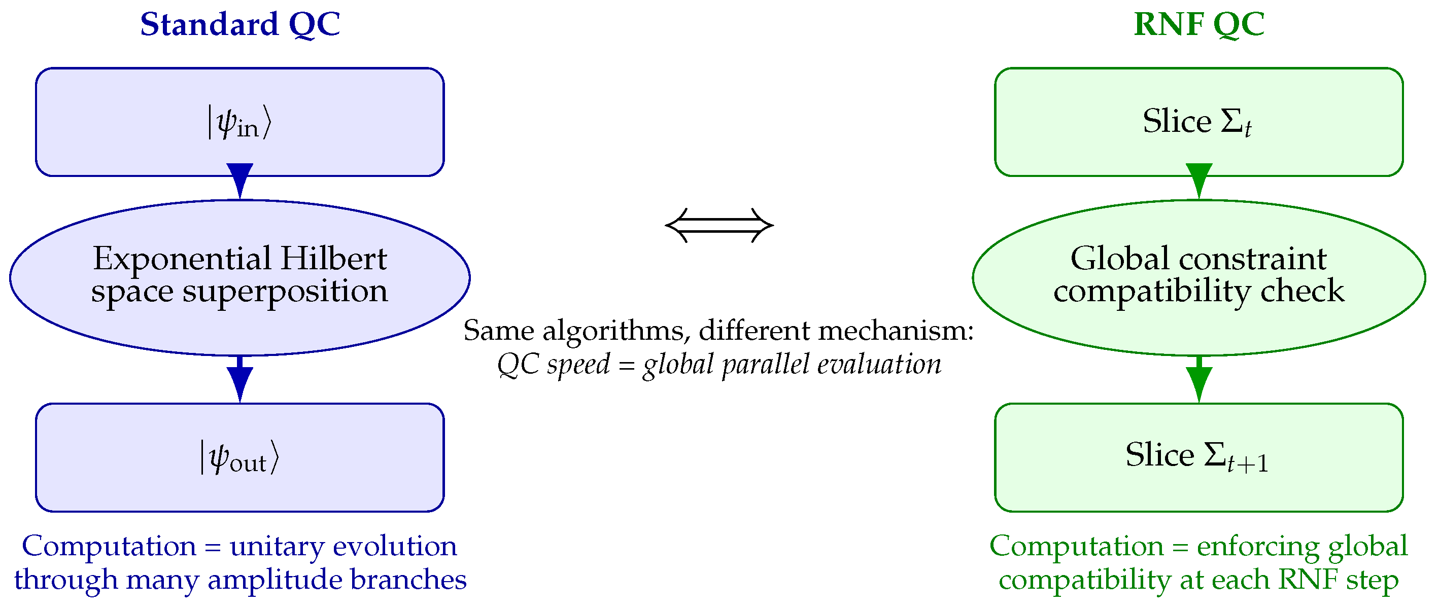
Comparison of standard quantum computation (QC) with the RNF view. Standard QC interprets speedup as evolution through an exponentially large superposition. In contrast, RNF QC interprets speedup as a single act of global constraint enforcement in 4D at each reconstruction step.
Figure 10.
Comparison of standard quantum computation (QC) with the RNF view. Standard QC interprets speedup as evolution through an exponentially large superposition. In contrast, RNF QC interprets speedup as a single act of global constraint enforcement in 4D at each reconstruction step.
9. Historical Context and Comparison with Standard Approaches
Since the birth of quantum theory, the phase factor has been accepted as a primitive rule rather than as the consequence of a deeper structure. Planck’s quantum of action h [54], Bohr’s quantized orbits [14], de Broglie’s matter waves [22], and Feynman’s path integral formulation [28,29] all rely on this phase. Yet none answered the structural question: why should nature assign probabilities through complex action–dependent phases?
The compact–action framework developed here provides such an answer. Once the action is intrinsically periodic—taking values on a compact domain rather than on —interference and phase addition arise as geometric necessities rather than postulates. Chronon Field Theory supplies the microscopic origin of this periodicity: the chronon medium carries a finite, topologically protected unit of symplectic twist, which endows the action with its compact structure. In this view, Planck’s constant reflects a geometric property of the underlying field, and the familiar quantum phase rules follow directly from the topology of the chronon medium rather than from ad hoc quantization assumptions.
9.1. Relation to Standard Quantum Mechanics
Standard quantum mechanics is structured around four elements: (i) complex state vectors, (ii) phase factors , (iii) unitary evolution, (iv) Born probabilities.
In the compact–action/RNF framework these arise from the geometry:
- The phase rule follows from action compactification (Section 4 and Appendix C).
- The path integral emerges from RNF summation over modular-equivalent families (Section 7).
- The Schrödinger equation appears in the long-wavelength, slowly-varying limit of RNF locality (Appendix J).
- The Born rule is recovered as a compatibility-basin measure during RNF alignment (Appendix I).
Thus standard quantum mechanics is not assumed but recovered as the effective description of compact action and RNF propagation.
9.2. Relation to Quantum Field Theory
Quantum field theory (QFT) quantizes classical fields on a fixed spacetime background and treats ℏ as externally supplied. In ChFT:
- arises from quantized symplectic flux;
- the spacetime metric is generated by RNF alignment of ;
- gauge interactions originate from holonomy of the polarization bundle.
In the appropriate geometric limit—large alignment scale and small curvature—aligned chronon configurations reproduce Einstein–Yang–Mills–type dynamics [42]. QFT is therefore obtained as an effective field theory whose fundamental parameters (action quantum, metric structure, and gauge couplings) have geometric origins in the chronon medium.
9.3. Why This Is Not an “Interpretation” of Quantum Mechanics
Interpretations of quantum mechanics retain the standard formalism and reinterpret its meaning. The compact–action/RNF/ChFT framework modifies the underlying structure:
- the phase is derived from compact geometry;
- interference arises from finite symplectic flux, not from wave duality;
- measurement corresponds to RNF compatibility selection, not a postulated collapse;
- spacetime, gauge fields, and matter solitons emerge from a common chronon dynamics.
The framework is therefore a geometric extension of quantum mechanics rather than a reinterpretation of its existing axioms.
9.4. Summary
The compact–action/RNF framework recovers all experimentally established predictions of quantum mechanics and quantum field theory while providing structural elements absent from the standard formalisms: a geometric origin of ℏ, an explanation for complex phases, a physical mechanism for measurement, and a unified emergence of spacetime, matter, and gauge structure from a single causal medium. It fits within the established theoretical landscape while completing elements that previously functioned only as axioms.
10. Conclusions
We have shown that a finite quantum of action , arising from the quantized symplectic flux of the chronon field, compactifies the action manifold from to and thereby enforces the phase structure underlying all quantum interference. Within this compact–action geometry, the Real–Now–Front (RNF) provides a local reconstruction rule that propagates only chronon-pattern trajectories lying in the same modular action class, recovering the structural forms of the Feynman path integral, the Schrödinger equation, and the Born rule. Interference, measurement, and entanglement arise from compatibility constraints during RNF alignment rather than from additional axioms.
A central feature is that each RNF slice represents the actual three-dimensional present—the advancing boundary at which new spacetime, matter patterns, and causal relations are brought into existence. This provides a concrete mechanism for Becoming, avoids the static block-universe picture, and supplies a physical selection rule ensuring macroscopic definiteness without invoking external observers. Because all observable excitations are emergent patterns on the RNF slice, the preferred direction of the chronon medium remains operationally concealed, yielding effective Lorentz invariance at all accessible energies.
In this sense, the compact–action/RNF framework functions not as an interpretation of quantum mechanics but as a geometric completion of it: Planck’s constant, quantum phases, causal structure, measurement, and the emergence of classical spacetime follow from the same underlying principles of symplectic quantization and RNF compatibility. The same reconstruction principle also ensures that information is preserved across horizons, eliminating the black–hole information paradox without additional hypotheses.
Future work will develop quantitative predictions of RNF quantum dynamics at high curvature and short distances, refine the soliton description of matter—including the minimal-soliton identification of the electron—and explore phenomenological consequences in mesoscopic interferometry, horizon physics, and possible chronon-scale effects.
Falsifiability. Although many chronon–scale effects lie beyond present technology, the framework makes several sharp and experimentally meaningful predictions. (1) ChFT implies an exponential suppression of Hawking-like emission; a clear detection of the standard Hawking spectrum or rapid evaporation of sub-stellar black holes would contradict this mechanism. (2) If collider or scattering experiments establish an electron compositeness radius much larger than the predicted chronon-scale value , the minimal-soliton identification would be ruled out. (3) If Lorentz invariance were found to fail at scales far above the chronon length , this would contradict the Co-moving Concealment Principle, which predicts effective Lorentz symmetry on all RNF slices. (4) If gravitational degrees of freedom were ever shown to become entangled, this would falsify the RNF prediction that only internal chronon-bundle modes can support quantum entanglement.
Any one of these observations would falsify core components of the chronon framework. Together they outline clear and testable criteria for assessing the viability of the compact–action/RNF program.
Author Contributions
Bin Li is the sole author
Funding
This research received no external funding
Abbreviations
The following abbreviations are used in this manuscript:
| ChFT | Chronon Field Theory |
| TCP | Temporal Coherence Principle |
| CCP | Co-moving Concealment Principle |
| RNF | Real Now Front |
Appendix A. TCP Mathematical Framework
This appendix summarizes the minimal mathematical structures of the Temporal Coherence Principle (TCP) needed for the compact–action geometry, the emergence of , and the RNF-based reconstruction rules used in the main text. We focus on configuration space, compatibility sets, and the symplectic twist structure; detailed topology, soliton stability, and RNF dynamics appear in later appendices.
Appendix A.1. Configuration Space of Chronon Fields
Let be a smooth four-dimensional manifold. A chronon field is a smooth unit timelike covector
and the configuration space is
A chronon pattern on is a map , whose spatial gradients encode twist, alignment, and curvature. A pattern is called aligned when is small in an appropriate norm, enabling the construction of an emergent metric.
Appendix A.2. Compatibility Sets
To each pattern the TCP dynamics assigns a compatibility set
Two patterns are compatible when
This structural notion underlies the distinctions between interference (overlapping compatibility), decoherence (environmental elimination of overlap), measurement (selection of a single surviving class), and entanglement (joint constraints). No Hilbert-space or probabilistic assumptions are needed at this stage.
Appendix A.3. Symplectic Twist and the Emergence of ℏgeom
The TCP dynamics includes the universal antisymmetric two-form
whose flux around closed loops defines the symplectic twist
Quantization follows from three structural features:
- (i)
- finite-energy configurations compactify spatial infinity, placing chronon fields into homotopy classes labeled by n;
- (ii)
- the twist bundle associated with has compact topology;
- (iii)
- quartic TCP terms prevent continuous unwinding of twist.
Thus is the minimal symplectic increment of , determined by the stabilized core structure of TCP solitons. Its later appearance in compact action and RNF propagation requires no Hilbert space: it follows from the topology and stabilization properties of .
Appendix A.4. TCP Action and Field Equation
The Temporal Coherence Principle is encoded in the action
where:
- controls temporal alignment,
- controls antisymmetric twist,
- supplies quartic stabilization,
- enforces .
A representative quartic term is
the lowest-order local scalar providing the required Derrick-stabilizing stiffness. Its variation yields the nonlinear term in the TCP equation.
Varying the action gives the unified TCP field equation:
In low-curvature, slowly varying regimes:
- the symmetric sector of (A.6) yields Einstein-like geometry (Appendix E),
- the antisymmetric sector produces Yang–Mills–like curvature evolution (Appendix D),
- the scalar sector reproduces Schrödinger dynamics (Appendix J).
Quantum dynamics, gauge interactions, and spacetime geometry therefore emerge as effective limits of the same underlying TCP equation.
Remarks on the Lagrangian.
The functional (A.5) is not unique; it is a minimal representative of a broader universality class of chronon actions that all share three structural features: (i) local alignment dynamics, (ii) a quantized twist sector, and (iii) quartic stabilization ensuring finite-energy solitons and a compact action manifold. More general Lagrangians may be constructed, but their long-wavelength limits coincide with those derived here.
Appendix A.5. Summary
This appendix supplies the minimal mathematical structures required for the later technical results:
- configuration space of unit timelike chronon fields;
- definition of chronon patterns and alignment criteria;
- TCP compatibility sets underlying interference, entanglement, and measurement;
- symplectic twist and the geometric origin of ;
- and the TCP action enforcing coherence, curvature control, and soliton stabilization.
These ingredients form the substrate for the compact-action theorem, RNF reconstruction dynamics, and the emergence of quantum and gravitational behavior developed in the main text.
Appendix B. The RNF Reconstruction Map
This appendix summarizes the minimal mathematical structure of the Real–Now–Front (RNF) reconstruction rule used in the main text. The RNF acts as a local update operator that converts pre-geometric chronon microstates into aligned chronon fields on the next geometric slice. No global memory structure, blueprint, or nonlocal object is assumed. All global correlations are preserved solely because the aligned slice already encodes them locally.
Appendix B.1. Pre-Geometric Microstate Domain
Let denote the pre-geometric reservoir ahead of the RNF. Elements
represent raw chronon microstates with no spatial metric, adjacency, or topological structure. Geometry, distance, and gauge data appear only after alignment through the TCP energy dynamics.
Appendix B.2. Local Compatibility
Let denote the aligned chronon pattern on the current slice . A pre-geometric microstate is compatible with at a point x if locally:
Here is a small neighborhood in the pre-geometric domain and is the TCP energy density. Only microstates that can extend the local twist, polarization, and alignment structure of qualify as compatible.
Importantly, the compatibility condition is purely local. No global object is stored or transported. Global correlations—including entanglement, holonomy, and flux—are preserved because they are already encoded in the local pattern itself.
Appendix B.3. The RNF Alignment Operator
At each point of the next slice the RNF applies a local alignment map:
The value of at is defined by:
subject to the following constraints:
- Locality: Only influences the update at .
- Compatibility: The map is defined only for microstates that are compatible with .
- Minimal TCP energy: Among compatible candidates, the RNF selects the one minimizing local TCP energy density.
No Hilbert-space amplitudes or propagation rules are assumed. The RNF is purely a geometric alignment rule.
Appendix B.4. Parallel Reconstruction and Absence of Preferred Points
The RNF assigns values at all points simultaneously. There is no preferred update point and no propagation order. This parallelism is essential: it ensures that global correlation structures—such as entanglement constraints linking distant regions— are reconstructed automatically, because the existing slice itself provides the local compatibility conditions that encode these correlations.
Thus:
- no global correlation object is stored,
- no nonlocal signal is transmitted,
- the entire constraint network reappears because it is already encoded locally everywhere on ,
- and the RNF applies the same local rule in parallel at all points.
This resolves apparent tensions with relativity: the RNF does not send signals through spacetime; it generates spacetime.
Appendix B.5. Transport and the Emergence of Motion
Motion and wave propagation appear through a geometric transport map
determined by minimizing incremental TCP energy subject to compatibility. Pattern elements shift by
defining the emergent shift vector .
Transport and local alignment together generate:
- soliton motion (drift of curvature cores),
- wave propagation (coherent variations of ),
- and preservation of all correlation constraints.
Appendix B.6. Causality
RNF updates take place in the pre-geometric domain . Since the update at depends only on , the RNF does not transmit information across spacelike regions of the emergent metric. After alignment, all fields propagate causally via the hyperbolic TCP equations on the emergent Lorentzian geometry.
Appendix B.7. Summary
The RNF reconstruction rule consists of:
- a pre-geometric microstate domain without spatial structure,
- local compatibility constraints derived from the TCP energy,
- a strictly local alignment map ,
- parallel reconstruction at all points of ,
- and a transport map generating motion and wave propagation.
Global correlations on are automatically preserved because they are expressed as local compatibility relations everywhere on the slice. The RNF therefore reconstructs the entire geometric world at each step using only local, energy-minimizing rules, without storing or communicating nonlocal information.
Appendix C. Topological Structure of the Chronon Field
In this appendix we develop the topological underpinnings of the chronon field, establish the configuration space in which finite-action configurations reside, derive the homotopy classification of admissible patterns, and demonstrate that the symplectic flux associated with polarization of the chronon field is quantized. This analysis provides the mathematical foundation for the existence of a fundamental quantum of action and explains why the relevant winding number is uniquely .
Throughout this appendix, denotes the smooth, future-directed, unit-norm timelike chronon field, and the induced spatial projector orthogonal to . The polarization structure arises from local deformations of the transverse two-dimensional subspace orthogonal to the instantaneous motion of . The twist and curvature of polarization encode the internal geometric structure responsible for quantized flux.
Appendix C.1. Configuration Space and Polarization Bundle
A chronon configuration consists of a smooth, unit-norm, timelike vector field on a four-dimensional manifold M, subject to the constraint
The orthogonal complement of defines a spatial subspace
with projector . The polarization degrees of freedom reside in a two-dimensional subbundle , with local orthonormal frame , . The frame is defined modulo local rotations, giving a natural fiber at each spacetime point.
Appendix C.2. Homotopy Classification of Chronon Patterns
Topologically nontrivial configurations arise as continuous maps from closed two- or three-dimensional surfaces into the space of polarization frames. The polarization fiber has the standard homotopy groups
but the physically relevant topology arises from its embedding in the orientation two-sphere associated with the spatial subbundle. The resulting structures are the familiar nonlinear-sigma-model textures and vortices [46]:
which give
Finite-action chronon configurations approach constant polarization at spatial infinity, and therefore belong to homotopy classes in . The integer k counts the winding of the local polarization around the soliton core, analogous to the winding of baby-Skyrmions or Hopf textures [27].
Appendix C.3. Quantization of Symplectic Flux
The polarization bundle carries a natural connection
whose curvature two-form is
The symplectic flux through a closed two-surface is
Theorem C.1
(Topological Flux Quantization). For any closed surface Σ surrounding a finite-action chronon configuration,
where k is the winding number of the induced map .
Proof.
Since is the curvature of a connection, its integral obeys the Chern–Weil quantization condition [19,48]:
where is the area form on the unit two-sphere. Integrating yields the integer degree of the map n:
□
Thus is a homotopy invariant labeling topological sectors of the chronon field.
Appendix C.4. Uniqueness of the Fundamental Winding Number k = 1
Although allows infinitely many winding sectors, three physical principles restrict physically realized chronon solitons to :
(i) Additivity.
Well-separated solitons must satisfy additive flux, excluding noninteger or fractional winding.
(ii) Energetic stability.
For sigma-model-type solitons, gradient energy grows as [23]. Thus configurations are unstable to fission into k separate solitons.
(iii) Phase periodicity.
The experimentally observed phase periodicity of interference is only consistent with the fundamental sector; higher k would induce additional modular periodicities not observed.
Thus stable, finite-action chronon solitons inevitably carry the unique fundamental topological charge , corresponding to one unit of symplectic flux .
Appendix C.5. Collective Accumulation: A Minimal Soliton–Gas Model
The preceding subsection established that higher–winding configurations () are energetically unstable, with gradient energy scaling as , and therefore factor into k well-separated unit-winding solitons. As a result, the physically realized sector is , with each chronon soliton carrying a single quantum of geometric action .
To explain how macroscopic classical actions arise, we introduce a coarse-grained “soliton–gas” model. Consider a spacetime domain D containing N well-separated unit-winding solitons with local number density . Because the symplectic flux is additive under concatenation of disjoint cores, the total flux threading any enclosing surface is
where is the chronon symplectic 2-form defined in Appendix M.2.
Define the coarse-grained action (or flux) density
For any macroscopic process described by a world-tube intersecting D, the effective accumulated action is then
which can be arbitrarily large even though each microscopic constituent contributes only a single quantum .
This construction shows explicitly that classical actions originate from the coherent accumulation of many unit-winding solitons rather than from single solitons with higher topological charge. In the limit of large N, the modular structure (with spacing ) becomes operationally negligible, reproducing the smooth classical behavior discussed in Appendix R.
Appendix D. Gauge Holonomy and the Standard Model Sector
Gauge interactions arise from the holonomy of the polarization bundle defined by the chronon field[42]. Internal rotations of the transverse polarization frame form a compact structure group whose connection induces the familiar gauge potentials, in direct analogy with the standard geometric formulation of gauge theory [48,69]. Nontrivial holonomy then yields emergent , , and sectors, and the long-wavelength reduction of the associated curvature reproduces the Yang–Mills action [66,70].
Appendix D.1. Polarization Bundle and Transverse Structure
As described in Appendix C, the chronon field defines a spatial projector and a transverse polarization subbundle . A local orthonormal frame , , satisfies
Local rotations of the polarization frame act by
identifying the polarization bundle as a principal bundle with intrinsic connection and curvature [48]. If the transverse internal space is enlarged (e.g., two or three complex polarization modes), the structure group generalizes to or accordingly.
Appendix D.2. Holonomy of the Polarization Connection
Given a polarization frame, the associated bundle connection is
which transforms as a gauge field under internal frame rotations [69]. The curvature is
and the holonomy of a closed loop ,
encodes the emergent gauge flux.
The structure group of the polarization fiber determines the effective gauge group: a one-mode complex fiber yields , a two-mode fiber yields , and a three-mode fiber yields —precisely the compact groups acting transitively on 1-, 2-, and 3-dimensional complex spheres.
Appendix D.3. Emergence of U(1), SU(2), and SU(3)
1. U(1) sector.
A single complex polarization mode gives a connection with curvature
interpreted as the Abelian gauge field.
2. SU(2) sector.
Two degenerate polarization directions define an fiber. The traceless part of gives an emergent weak-isospin connection
with non-Abelian curvature.
3. SU(3) sector.
Three polarization modes generate an connection
providing an emergent color gauge field analogous to QCD [66].
Thus the Standard Model group
arises as the minimal compact structure group compatible with soliton propagation in a three-dimensional complex polarization fiber.
Appendix D.4. Long-Wavelength Reduction to Yang–Mills Form
At scales large compared to the soliton core, polarization variations are slow, and the leading contribution to the action comes from the curvature of the polarization connection. By expanding the chronon action to quadratic order in transverse fluctuations, the effective action becomes
which is the universal Yang–Mills form [70]. Higher-order terms encode suppressed chronon-structure corrections. A fully covariant derivation requires detailed decomposition of the polarization bundle, which will be presented separately.
Appendix E. Coarse-Grained TCP Dynamics and Einstein Geometry
The chronon field induces a natural foliation of spacetime into three-dimensional slices orthogonal to , together with an effective spatial geometry. In this appendix we show how the Temporal Coherence Principle (TCP), coarse-grained over scales large compared to the soliton core, yields Einstein-like gravitational dynamics. Our construction follows the standard 1+3 covariant decomposition and foliation geometry used in general relativity [3,25,33]. We first decompose derivatives along and orthogonal to , then introduce a macroscopic averaging scheme appropriate for TCP dynamics, and finally derive the emergent Einstein equations and identify the relation between chronon stiffness parameters and the effective gravitational and cosmological constants.
Appendix E.1. Projection Along and Orthogonal to Φμ
The chronon field is a smooth, future-directed unit timelike vector:
The orthogonal projector
splits tensors into components parallel and orthogonal to . The covariant derivative decomposes as
where the acceleration, expansion, shear, and vorticity are the standard kinematical quantities of a timelike congruence [25]. The tensor
acts as the extrinsic curvature of the spatial slices [33].
Appendix E.2. Averaging and Hydrodynamic Limit
Microscopically, TCP dynamics include strong gradients and soliton cores. To obtain macroscopic gravitational behavior we apply a spatial coarse-graining over a domain whose size lies between the soliton scale and curvature scale, following cosmological averaging methods [16].
For any scalar X:
An effective macroscopic metric is defined by requiring:
(i) ,
(ii) hypersurface orthogonality after averaging,
(iii) is the induced spatial metric,
(iv) the Levi–Civita connection of minimizes higher-derivative distortions of the averaged chronon alignment.
These conditions yield a consistent coarse-grained curvature tensor .
Appendix E.3. Effective Einstein Equations
The microscopic TCP action contains quadratic terms in , , , and . Upon averaging, only the quadratic pieces survive at long wavelength.
Theorem E.1
(Emergent Gravitation). Under coarse-graining, the TCP field equations reduce to
where is the coarse-grained chronon stress tensor. Both and are determined by the chronon stiffness coefficients.
Quadratic chronon deformation terms serve as sources, yielding (E.16). Higher-derivative TCP contributions are suppressed at large scales. A similar emergence of Einstein dynamics from microscopic alignment laws appears in related contexts [39]. □
Appendix E.4. Relation Between (J,λ,α,κ) and (G,Λ)
The coefficients in the chronon action determine the effective gravitational couplings.
Effective Newton constant.
The extrinsic-curvature part of the action is
Matching with the Gauss–Codazzi structure gives
with constants of order unity determined by the averaging domain.
Effective cosmological constant.
Shear and vorticity contribute a background energy density
Hence
If becomes fully aligned, decays; if alignment is incomplete, a residual term remains.
Thus determine , while determine via residual chronon deformation energy.
Appendix F. Existence and Stabilization of Chronon Solitons
Chronon solitons play a foundational role in the compact–action/RNF framework: they provide finite-energy, finite-size excitations of the chronon medium and supply the quantized symplectic flux underlying the action compactification theorem. The mechanism summarized here follows the standard topological–solitonic framework developed in nonlinear field theory [46].
Appendix F.1. Finite-Energy Boundary Conditions and Topological Charge
A finite-energy configuration requires that approach perfect alignment at spatial infinity. This compactifies spatial infinity to , so any static finite-energy configuration defines a map
labeled by an integer degree n. The antisymmetric gradient of defines the twist two-form
whose flux through any closed surface enclosing the core satisfies
As in other topological soliton systems, this integer is protected against continuous finite-energy deformations [46].
Appendix F.2. Derrick Scaling and the Need for Quartic Stabilization
In three spatial dimensions, Derrick’s theorem [23] implies that purely quadratic gradient theories cannot support stable, static, finite-size solitons: under the scaling , the quadratic energy scales as
Chronon Field Theory avoids collapse because the TCP action includes a quartic contribution of the schematic form
scaling as
Appendix F.3. Existence of Finite-Radius, Finite-Energy Solutions
Combining topological charge with Derrick-stabilized energy yields the existence of finite-energy solitons:
1. Finite-energy boundary conditions compactify space to , placing configurations in sectors labeled by .
2. Quartic TCP terms prevent collapse under scaling, ensuring that each topological sector has a nonzero minimal length scale.
3. The energy functional is smooth and bounded below within each sector.
4. Each sector therefore admits at least one finite-radius minimizer, a chronon soliton carrying charge n.
This parallels existence results in other stabilized topological models [2].
Figure A1 is a schematic illustration of the stabilization mechanism.
Appendix F.4. Rigorous Dynamical Stability (Cross-Reference)
Appendix G analyzes the dynamical and perturbative stability of these solutions, showing that
- topological charge is exactly conserved under RNF evolution, - boosted solitons form a smooth moduli space, and - small perturbations decompose into localized shape modes and radiative modes.
Thus solitons are not only admissible solutions but stable, particle-like excitations of the chronon medium.
Remark.
A complete global PDE proof of stability for all topological sectors requires advanced methods in nonlinear hyperbolic systems and is deferred to future work.
Figure A1.
Left: Without the quartic TCP term the TCP energy functional obeys Derrick scaling, so the chronon configuration collapses to zero size. Right: The quartic term introduces an outward restoring force that balances inward curvature pressure, stabilizing a preferred soliton core radius . This stabilized soliton carries a quantized symplectic flux , providing the geometric quantum of action that underlies compactified action space.
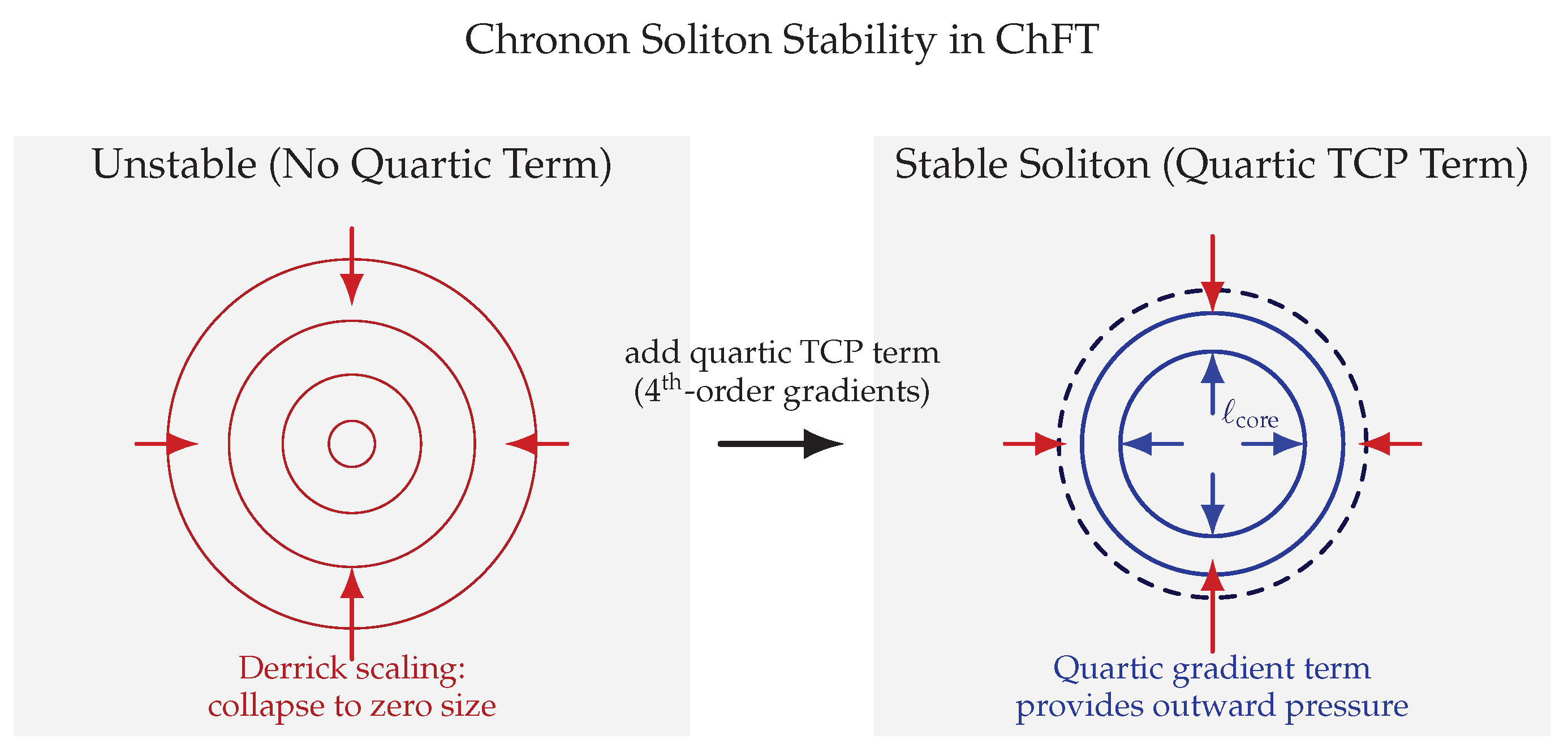
Appendix G. Dynamical Stability of Chronon Solitons
Chronon solitons arise as finite-action, topologically nontrivial solutions of the TCP equations, stabilized by quartic terms and carrying unit winding number. In this appendix we show that such solitons remain well-defined under time evolution, admit boosted (traveling) solutions, and are stable to small perturbations. The structure closely parallels standard results in soliton dynamics and moduli-space evolution [45,46,61].
Appendix G.1. Boosted Soliton Solutions as Slice-by-Slice Reconstruction
Let denote a static soliton solution centered at the origin and approaching perfect alignment at spatial infinity. In the RNF formulation, motion corresponds to the soliton core being reconstructed at shifted positions on successive slices,
In the long-wavelength regime, where the RNF advances smoothly, these slice-by-slice reconstructions assemble into an effective four-dimensional configuration on the emergent Lorentzian geometry. A soliton moving with constant velocity v takes the boosted form
analogous to the moduli-space construction for classical solitons [46]. Because the TCP action becomes locally Lorentz-invariant in the coherent limit, satisfies the same field equations as the static solution.
To leading order, the soliton center follows the effective worldline
with higher-order corrections suppressed by the inverse soliton size. This is precisely the moduli-space approximation familiar from classical soliton dynamics [45].
Appendix G.2. Conservation of Topological Charge Under Motion
Let be the symplectic curvature two-form of the polarization bundle and a closed two-surface enclosing the soliton on slice t. The topological charge is
Since and the soliton remains isolated, the flux through is independent of t:
Thus k is exactly conserved, as in all finite-energy topological soliton systems [46]. Deformations or accelerations cannot change the charge unless another topological defect crosses the enclosing surface.
Appendix G.3. Perturbative Analysis and Dispersion Relations
Consider linearized fluctuations about a static soliton,
The constraint imposes to first order. Inserting the expansion into the TCP equations gives the linearized operator
Far from the core, where the background is approximately aligned, the operator reduces to a wave operator on ,
yielding the dispersion relation
Appendix G.4. Time-Dependent Stability Theorem
Theorem G.1
(Soliton Stability Under Evolution). Let be a finite-action, unit-winding chronon soliton. For sufficiently small perturbations satisfying , the following hold:
- The perturbed solution exists globally in time (no finite-time blowup).
- The topological charge is exactly conserved:
-
The evolving solution remains close to the soliton moduli space:with smooth functions and .
- All linear perturbations decompose into localized massive shape modes plus dispersive radiative modes satisfying .
Thus chronon solitons are nonlinearly stable and behave as coherent, particle-like excitations of the chronon field.
Appendix H. Classical Limit and Effective Decompactification of Action
A key feature of the chronon framework is that the quantum of action is a fixed geometric invariant set by the minimal symplectic flux of a chronon soliton. Unlike in heuristic path–integral arguments, the classical limit does not correspond to taking . Instead, exactly as in standard semiclassical analyses [29,57], the classical limit emerges when the granularity encoded by is unresolvable relative to the large actions and coarse observables involved.
In this regime, the modular identification becomes operationally irrelevant, and the action behaves effectively as a noncompact variable.
Appendix H.1. Fixed Geometric Origin of ℏgeom
The quantum of action is determined by the minimal symplectic flux carried by a chronon soliton,
and is set by microscopic stiffness parameters . Nothing in the dynamics drives toward zero. Thus the classical limit arises solely through coarse–graining and large actions, not through tuning .
Geometric origin of the factor. Although one could formally absorb numerical constants into a redefinition of , the compactification scale of the action is not a matter of convention. The fundamental periodicity arises from the twist of the chronon polarization bundle: a full rotation of the internal phase returns the polarization frame to itself, so the symplectic flux is quantized in units of . Thus the appearance of reflects intrinsic bundle topology rather than a convenient normalization chosen to match standard quantum mechanics.
Appendix H.2. Why Classical Phenomena Ignore Action Compactification
The RNF transition amplitude involves a circle–valued action,
In classical regimes:
- for all resolved histories,
- modular shifts produce phase changes far below experimental resolution,
- phase fluctuations average out over coarse observables.
Thus the compactification radius becomes operationally infinite: the circle is never probed at its true microscopic scale.
Appendix H.3. Effective Recovery of
Although formally S is circle–valued, classical measurements access only differences
where modular identifications are experimentally invisible. For all coarse observables, the action behaves like a real number, recovering the usual variational description of classical mechanics.
Appendix H.4. Classical Trajectories as Stationary RNF Reconstructions
The RNF transition amplitude is
Appendix H.5. Summary
The chronon framework preserves a fixed geometric quantum of action at all scales. The classical limit is recovered when:
- physical actions greatly exceed ,
- action compactification becomes experimentally irrelevant,
- phase averaging suppresses nonstationary RNF histories.
Thus classical mechanics emerges as the large–action, slowly varying limit of RNF quantum dynamics, mirroring the standard semiclassical transition but with a geometric, rather than postulated, origin of the action quantum.
Appendix I. RNF Probability Measure and the Born Rule
The Real–Now Front (RNF) selects, among all geometrically admissible chronon continuations, those configurations that maximize local compatibility with the previous slice. This induces a natural geometric measure on the space of admissible continuations. In this appendix we define compatibility basins, derive the induced probability weights, and prove that the RNF geometric measure yields the Born rule [15,32,65], in close analogy to geometric approaches based on envariance [72].
Appendix I.1. Compatibility Basins and Alignment Volumes
Let be an RNF slice and the space of geometrically allowed chronon configurations on the next slice . Each candidate configuration can be continued only if its polarization frame remains compatible with the existing chronon alignment.
Define the compatibility functional
measuring the geometric overlap between polarization projectors on consecutive slices.
For a macroscopic outcome O, define its compatibility basin
The RNF assigns weight
where is the volume element on configuration space and is the alignment sharpness parameter.
Scaling of compatibility volume.
Within a measurement context, the RNF restricts the pre-geometric configuration to the basin . Small variations of the incoming state modify only through its overlap with the branch vector . The admissible deformations form a codimension–one tubular neighborhood whose transverse radius scales as . Thus the RNF measure of the basin scales as
anticipating the Born rule.
Appendix I.2. RNF-Induced Probability Weights
Lemma A1.
Let be the alignment volume (I.17). Then
The probability ratio between two outcomes is
Proof.
Normalization is immediate. Since incompatible configurations contribute negligibly, probability ratios depend only on relative alignment volumes. □
Appendix I.3. Born Rule for RNF Alignment
Theorem I.1
(RNF Born Rule). Let be the incoming polarization state on , and let be the RNF-induced alignment volume of the compatibility basin . In the strong-alignment limit, the RNF probability of outcome O is
Thus the RNF geometric measure reproduces the Born rule.
Appendix I.4. Derivation of |ψ|2 from Geometric Measure
Let outcome O correspond to a polarization state on the slice , normalized by .
For , the geometric overlap is, for large alignment sharpness ,
so
All configurations in satisfy , so
Hence
where is the geometric volume of .
But itself scales as because the tubular neighborhood of compatible configurations has transverse radius . Thus
Appendix J. Nonrelativistic Limit and Schrödinger Dynamics
The RNF formalism defines a transition amplitude between chronon-aligned configurations as a sum over all geometrically admissible microcontinuations, each weighted by the compactified action phase. When macroscopic changes over a single RNF step are small compared to the chronon coherence scale, this amplitude admits a short-time expansion analogous to the Feynman short-time kernel [29,57]. In this appendix we show that the RNF kernel reduces to the standard nonrelativistic propagator and that the Schrödinger equation emerges as the continuum limit of RNF dynamics.
Appendix J.1. RNF Propagator and Short-Time Kernel
Let denote the RNF transition amplitude for an excitation of effective mass , moving in a potential , between two positions on successive RNF slices. By definition,
where the sum is over all RNF-compatible microhistories connecting the two boundary points.
For sufficiently small , the action is dominated by the kinetic term:
Thus the RNF kernel takes the short-time form
with normalization factor (fixed by RNF measure preservation)
Appendix J.2. Expansion of the Action Around the Classical Path
Let be the classical path between the endpoints, satisfying . Fluctuations are parametrized as
Expanding the action to quadratic order,
where is the second functional derivative of S. The linear term vanishes because extremizes the action.
Thus the RNF propagator becomes
Appendix J.3. Recovery of the Schrödinger Equation
Let be the RNF-induced wave amplitude on slice t. Propagation to the next slice yields
Substituting the kernel (J.18) and expanding to first order in gives
Taking the limit yields the Schrödinger equation:
Theorem J.1
(Nonrelativistic Limit). Let the RNF coherence scale exceed the spatial variation scale of ψ, and let be finite. Then the RNF transition amplitude for an excitation of effective mass reduces, in the limit , to the Schrödinger evolution law:
Thus nonrelativistic quantum mechanics emerges as the continuum limit of RNF dynamics under mild smoothness and coherence assumptions.
Appendix K. Fermionic Degrees of Freedom as Chiral Twist Defects
The chronon field admits topologically stable solitons characterized by a unit winding number. When embedded in the polarization bundle, these solitons can support additional internal twist structures. In this appendix we show that such twist defects give rise to fermionic degrees of freedom, realized as chiral edge modes bound to soliton boundaries. This mechanism parallels well-known constructions in topological field theory where solitonic defects host fermionic zero modes [17,38,48]. The resulting excitations behave as effective spin- modes whose dynamics naturally couple to the gauge holonomy derived in Appendix D.
Appendix K.1. Motivation and Conceptual Basis
Chronon solitons are localized, finite-action configurations stabilized by their topological winding number. Placing such a soliton inside the polarization bundle allows the surrounding polarization frame to carry nontrivial twist patterns. These twist patterns support gapless, chiral excitations localized near the soliton boundary.
A fermionic degree of freedom corresponds to a chiral twist defect bound to the boundary of a chronon soliton. The twist reverses sign under a rotation, giving the mode an emergent spin- character.
Appendix K.2. Chiral Edge Modes on Soliton Boundaries
Let be a unit-winding soliton and let be a thin tubular neighborhood around its core. On the boundary , the polarization frame defines a local fibration. A twist defect corresponds to a phase rotation of this frame,
The half-odd periodicity forces any mode bound to the defect to pick up a minus sign after a rotation.
Linearizing the dynamics near yields an effective one-dimensional Hamiltonian similar to that appearing in soliton-bound fermionic modes [38]. The eigenmodes take the form
so the anti-periodic boundary condition encodes the spinor nature of the mode.
Appendix K.3. Spin-1 2 from Polarization–Twist Pairing
Let be the polarization connection. The holonomy around the soliton boundary is
A twist defect changes the trivialization of the bundle, producing a phase
under a rotation. Thus the corresponding boundary mode transforms as
exactly as a spin- state transforms under full rotation.
The twist cannot be removed without unwinding the soliton core, so the spinor mode is topologically protected. This mirrors index-theoretic arguments for fermionic zero modes on solitons [68].
Remark on Pauli exclusion.
The chiral twist supports a single normalizable edge mode whose wavefunctional reverses sign under a rotation. In the RNF framework, exchanging two such solitons traces a nontrivial loop in the configuration space that induces the same sign reversal. Consequently, multi-soliton states are antisymmetric under exchange, providing a geometric implementation of Pauli exclusion without imposing anticommutation relations externally.
Appendix K.4. Coupling Between Fermionic Modes and Gauge Holonomy
Because the fermionic mode is localized on and tied to the polarization bundle, it couples naturally to the gauge connection .
Parallel transport around the boundary acts as
Expanding for small loops gives the familiar minimal coupling:
If the polarization bundle has non-Abelian structure, e.g. or , the holonomy acts on the corresponding internal representation. Thus the twist-bound fermionic mode couples to gauge fields through the same geometric mechanism that yields vector bosons in Appendix D. The interaction is purely geometric and requires no independent matter fields.
Appendix L. RNF Horizon Emission: Quantitative Suppression Mechanisms
This appendix provides a quantitative upper bound on possible horizon–scale emission in the RNF/ChFT framework. Because the vacuum is a fully aligned chronon configuration with no free modes, pair creation, or high–frequency fluctuations, emission can arise only from weak leakage of curvature–alignment waves. This leakage is limited by (i) chronon stiffness, (ii) the intrinsic UV cutoff of twist modes, and (iii) the one–sided alignment boundary at the horizon.
Appendix L.1. Absence of Standard Hawking Mode Mixing
Standard Hawking radiation relies on Bogoliubov mixing of linear quantum field modes under the exponential stretching with surface gravity [12,26,35]. This mechanism assumes:
- free propagating modes,
- vacuum fluctuations up to arbitrarily high frequency,
- efficient conversion of near-horizon curvature into long-wavelength quanta.
None of these assumptions apply in RNF/ChFT:
- excitations are chronon twist/curvature modes with a UV cutoff ,
- the vacuum is rigidly aligned (no virtual pairs),
- the horizon imposes a one-sided reconstruction boundary that damps long-wavelength twist.
Thus the horizon behaves not as a particle amplifier but as an alignment-equilibrium surface.
Appendix L.2. Misalignment Energy Near the Horizon
Let denote the aligned field just outside the horizon. Any attempted reconstruction across the near-horizon layer produces a TCP misalignment cost of the form
Near a Schwarzschild horizon the alignment gradients are expected to grow as
where p distinguishes longitudinal and transverse stiffness response. The relevant reconstruction layer has volume , giving the order-of-magnitude upper bound
This expression is not a precise formula but an estimate of how misalignment energy must scale with horizon size and alignment length.
Appendix L.3. Suppression of RNF Reconstruction Across the Horizon
The RNF reconstruction probability for a configuration requiring misalignment energy satisfies a generic exponential bound
Using (L.20) yields
where encodes order-unity geometric factors and chronon stiffness. For any macroscopic black hole,
which makes the suppression factor astronomically small.
This is an upper bound: the actual suppression may be even stronger, but cannot be weaker without violating RNF alignment consistency.
Appendix L.4. Upper Bound on RNF Emission Rate
The base leakage scale of curvature–alignment waves has the dimensional form
Multiplying by the suppression bound (L.21) yields the emission upper limit:
This replaces the Hawking scaling with an exponentially smaller bound.
Appendix L.5. Physical Interpretation
For stellar or larger black holes:
Thus astrophysical black holes are effectively non-radiating within RNF.
For microscopic black holes the bound weakens, making long-lived compact objects plausible—consistent with the MCC chronon-core picture in RNF cosmology.
Appendix L.6. Summary
The RNF/ChFT framework does not produce standard Hawking radiation. Instead, horizon emission is limited by a curvature–alignment process with a calculable exponential upper bound. Chronon stiffness, UV cutoff, and the one–sided reconstruction boundary combine to suppress macroscopic emission far below Hawking levels, while allowing slowly radiating microscopic objects. This bound is compatible with RNF reconstruction, horizon alignment, and global information preservation.
Appendix M. RNF Entanglement Compatibility: Proof Sketch
This appendix provides a concise derivation of the Entanglement Compatibility result stated in Section 7.7. The proof relies on the configuration spaces , compatibility sets , the RNF-induced measure , and the reconstruction map defined in Appendix B.
The goal is to show that a non-factorizable chronon pattern on two regions A and B generically yields joint outcome statistics that violate Bell-local decompositions of the form introduced by Bell [10] and CHSH [18], even though RNF dynamics remain strictly local and causal.
Appendix M.1. Non-Factorizable Patterns Yield Non-Product Compatibility Sets
Let be a chronon pattern on and its marginal restrictions.
Lemma A2.
If is non-factorizable, , then
Proof.
By definition, consists of all aligned fields whose twist and curvature textures satisfy all constraints of , including cross-constraints linking A and B. A configuration may satisfy and individually but violate a cross-constraint, so the admissible set is strictly smaller than the Cartesian product. □
Thus the geometry of the chronon pattern induces correlations without requiring any dynamical influence between A and B.
Appendix M.2. RNF Reconstruction Preserves Joint Constraints
The RNF update minimizes the TCP functional while preserving all boundary and texture constraints.
Lemma A3.
If is non-factorizable on , then the reconstructed pattern on is also non-factorizable, and
Proof.
Local RNF minimizers preserve the inherited TCP constraints. Cross-terms in remain constraints on any admissible field. Because the interior of is closed under TCP-preserving deformations, the reconstructed pattern retains the non-product structure. □
Thus RNF dynamics are strictly local yet preserve global relational constraints.
Appendix M.3. Joint Probabilities on Non-Product Compatibility Sets
Let be local settings and the corresponding response maps. The RNF joint distribution is
Lemma A4.
If is non-product, then cannot be written as any product measure on .
Proof.
Any product measure has support contained in a Cartesian product. Because the support of is a proper non-Cartesian subset (Lemma 1), no such product representation exists. □
Thus the obstruction to Bell-factorization arises already at the level of the support of the RNF measure.
Appendix M.4. Incompatibility with Bell-Local Hidden-Variable Models
A Bell-local model requires a decomposition of the form
and, by Fine’s theorem [30], such a decomposition is equivalent to satisfying all CHSH inequalities.
Lemma A5.
For non-factorizable , the RNF distribution cannot satisfy (B.1).
Proof.
If (B.1) held, then would admit a product decomposition , contradicting Lemma 3. Hence no Bell-local hidden-variable model can reproduce RNF statistics. □
Therefore the CHSH bound does not apply, and the RNF correlation functional
can exceed the Bell-local limit for suitable settings.
Conclusion
RNF entanglement arises from:
- geometric non-factorizability of ,
- preservation of this structure under RNF reconstruction,
- induced measures that cannot factorize, and
- incompatibility with Bell-local decompositions.
Thus RNF produces quantum-like entanglement and Bell inequality violations entirely through local geometric constraints, with no nonlocal signaling.
References
- Aaronson, S. “Why philosophers should care about computational complexity,” in Computability: Turing, Gödel, Church and Beyond; MIT Press, 2013; pp. 261–328. [Google Scholar]
- Adam, C.; Sanchez-Guillen, J.; Wereszczynski, A. Nonlinear field theory with a bounded topological charge. Phys. Rev. D 2012, 86, 105009. [Google Scholar] [CrossRef]
- Arnowitt, R.; Deser, S.; Misner, C. W. Dynamical Structure and Definition of Energy in General Relativity. Phys. Rev. 1959, 116, 1322. [Google Scholar] [CrossRef]
- ALEPH Collaboration, Search for compositeness in e+e-→e+e- at LEP. Phys. Lett. B 1998, 422, 384.
- Almheiri, A.; Marolf, D.; Polchinski, J.; Sully, J. Black Holes: Complementarity or Firewalls? JHEP 2013, arXiv:1207.312302, 062. [Google Scholar] [CrossRef]
- Aoyama, T. The anomalous magnetic moment of the muon and electron. Phys. Rept 2020, 887, 1–166. [Google Scholar] [CrossRef]
- Aspect, A.; Dalibard, J.; Roger, G. Experimental Test of Bell’s Inequalities Using Time-Varying Analyzers. Phys. Rev. Lett. 1982, 49, 1804. [Google Scholar] [CrossRef]
- ATLAS Collaboration, Search for excited electrons and muons in s=13 TeV pp collisions with the ATLAS detector. JHEP 2020, 12, 005. [CrossRef]
- Barceló, C.; Liberati, S.; Visser, M. Analogue gravity. Living Rev. Relativ. 2011, 14, 3. [Google Scholar] [CrossRef] [PubMed]
- Bell, J. S. On the Einstein–Podolsky–Rosen paradox. Physics 1964, 1, 195. [Google Scholar]
- Berry, M. V. Quantal phase factors accompanying adiabatic changes. Proc. R. Soc. Lond. A 1984, 392, 45. [Google Scholar]
- Birrell, N. D.; Davies, P. C. W. Quantum Fields in Curved Space; Cambridge Univ. Press, 1982. [Google Scholar]
- D. Bleecker, Gauge Theory and Variational Principles; Addison–Wesley, 1981.
- Bohr, N. On the constitution of atoms and molecules. Philos. Mag. 1913, 26, 1. [Google Scholar] [CrossRef]
- Born, M. Zur Quantenmechanik der Stoßvorgänge. Z. Phys. 1926, 37, 863. [Google Scholar] [CrossRef]
- Buchert, T. On average properties of inhomogeneous fluids in general relativity. Gen. Relativ. Gravit. 2000, 32, 105–125. [Google Scholar] [CrossRef]
- Callan, C. G.; Harvey, J. A. Anomalies and fermion zero modes on strings and domain walls. Nucl. Phys. B 1985, 250, 427–436. [Google Scholar] [CrossRef]
- Clauser, J. F.; Horne, M. A.; Shimony, A.; Holt, R. A. Proposed experiment to test local hidden-variable theories. Phys. Rev. Lett. 1969, 23, 880–884. [Google Scholar] [CrossRef]
- Chern, S.-S. On the curvatura integra in a Riemannian manifold. Ann. Math. 1945, 46, 674–684. [Google Scholar] [CrossRef]
- Christodoulou, D.; Tahvildar-Zadeh, A. On the asymptotic behavior of spherically symmetric wave maps. Duke Math. J. 1993, 71, 31–69. [Google Scholar] [CrossRef]
- CMS Collaboration. Search for excited leptons in the ℓℓγ final state at 13 TeV. JHEP 2019, 79. [Google Scholar]
- de Broglie, L. Recherches sur la théorie des quanta. Ann. Phys. 1924, 3, 22. [Google Scholar] [CrossRef]
- Derrick, G. H. Comments on nonlinear wave equations as models for elementary particles. J. Math. Phys. 1964, 5, 1252. [Google Scholar] [CrossRef]
- Dirac, P. A. M. Quantised singularities in the electromagnetic field. Proc. R. Soc. Lond. A 1931, 133, 60. [Google Scholar]
- Ellis, G. F. R.; van Elst, H. Cosmological Models (Cargèse Lectures 1998); Springer, 1999. [Google Scholar]
- Fabbri, A.; Navarro-Salas, J. Modeling Black Hole Evaporation; Imperial College Press, 2005. [Google Scholar]
- Faddeev, L.; Niemi, A. J. Stable knot-like structures in classical field theory. Nature 1997, 387, 58–61. [Google Scholar] [CrossRef]
- Feynman, R. P. Space–time approach to non-relativistic quantum mechanics. Rev. Mod. Phys. 1948, 20, 367. [Google Scholar] [CrossRef]
- Feynman, R. P.; Hibbs, A. R. Quantum Mechanics and Path Integrals; McGraw–Hill, 1965. [Google Scholar]
- Fine, A. Hidden variables, joint probability, and the Bell inequalities. Phys. Rev. Lett. 1982, 48, 291–295. [Google Scholar] [CrossRef]
- Frankel, T. The Geometry of Physics, 3rd ed.; Cambridge Univ. Press, 2011. [Google Scholar]
- Gleason, A. M. Measures on the closed subspaces of a Hilbert space. J. Math. Mech. 1957, 6, 885–893. [Google Scholar] [CrossRef]
- Gourgoulhon, E. 3+1 Formalism and Bases of Numerical Relativity. arXiv arXiv:gr-qc/0703035.
- Hawking, S. W. Black hole explosions? Nature 1974, 248, 30–31. [Google Scholar] [CrossRef]
- S. W. Hawking, Particle creation by black holes. Commun. Math. Phys. 1975, 43, 199–220. [CrossRef]
- Hawking, S. W. Breakdown of Predictability in Gravitational Collapse. Phys. Rev. D 1976, 14, 2460. [Google Scholar] [CrossRef]
- Horodecki, R.; Horodecki, P.; Horodecki, M.; Horodecki, K. Quantum entanglement. Rev. Mod. Phys. 2009, 81, 865–942. [Google Scholar] [CrossRef]
- Jackiw, R.; Rebbi, C. Solitons with fermion number. Phys. Rev. D 1976, 13, 3398. [Google Scholar] [CrossRef]
- Jacobson, T. Thermodynamics of spacetime: the Einstein equation of state. Phys. Rev. Lett. 1995, 75, 1260. [Google Scholar] [CrossRef] [PubMed]
- Joos, E.; Zeh, H. D. The emergence of classical properties through environment interaction. Z. Phys. B 1985, 59, 223. [Google Scholar] [CrossRef]
- Li, B. Emergence and Exclusivity of Lorentzian Signature and Unit-Norm Time from Random Chronon Dynamics. Reports in Advances of Physical Sciences 2025, 9, 2550022. [Google Scholar] [CrossRef]
- Li, B. Emergent Gravity and Gauge Interactions from a Dynamical Temporal Field. Reports in Advances of Physical Sciences 2025, 9, 2550017. [Google Scholar] [CrossRef]
- Liberati, S. Tests of Lorentz invariance: a 2013 update. Class. Quantum Grav. 2013, 30, 133001. [Google Scholar] [CrossRef]
- Littlejohn, R. G. The semiclassical evolution of wave packets. Phys. Rep. 1986, 138, 193–291. [Google Scholar] [CrossRef]
- Manton, N. S. A remark on the scattering of BPS monopoles. Phys. Lett. B 1982, 110, 54. [Google Scholar] [CrossRef]
- Manton, N.; Sutcliffe, P. Topological Solitons; Cambridge Univ. Press, 2004. [Google Scholar]
- Monroe, C.; Meekhof, D. M.; King, B. E.; Wineland, D. J. Demonstration of a Fundamental Quantum Logic Gate. Phys. Rev. Lett. 1995, 75, 4714. [Google Scholar] [CrossRef]
- Nakahara, M. Geometry, Topology and Physics, 2nd ed.; Taylor & Francis, 2003. [Google Scholar]
- OPAL Collaboration, Tests of the standard model from e+e-→e+e-. Eur. Phys. J. C 1999, 6, 1.
- Nielsen, M. A.; Chuang, I. L. Quantum Computation and Quantum Information; Cambridge University Press, 2010. [Google Scholar]
- Padmanabhan, T. Thermodynamical aspects of gravity: new insights. Rep. Prog. Phys. 2010, 73, 046901. [Google Scholar] [CrossRef]
- J. Pearl, Causality: Models, Reasoning, and Inference; Cambridge Univ. Press, 2009.
- Pinčák, R.; Pigazzini, A.; Pudlák, M.; Bartoš, E. Introduction of the G2-Ricci Flow: Geometric Implications for Spontaneous Symmetry Breaking and Gauge Boson Masses. Nuclear Physics B 2025, 1017, 116959. [Google Scholar] [CrossRef]
- Planck, M. On the law of distribution of energy in the normal spectrum. Ann. Phys. 1901, 4, 553. [Google Scholar] [CrossRef]
- H. Price, Time’s Arrow and Archimedes’ Point; Oxford Univ. Press, 1996.
- C. Rovelli, The Order of Time; Riverhead Books, 2018.
- Schulman, L. S. Techniques and Applications of Path Integration; Wiley, 1981. [Google Scholar]
- Shatah, J.; Strauss, W. “Spectral condition for instability,” in Nonlinear Dispersive Equations; 1998. [Google Scholar]
- Schrödinger, E. Discussion of Probability Relations Between Separated Systems. Proc. Camb. Phil. Soc. 1935, 31, 555–563. [Google Scholar] [CrossRef]
- Skyrme, T. H. R. A nonlinear field theory. Proc. R. Soc. A 1961, 260, 127. [Google Scholar]
- Stuart, D. The geodesic approximation for the Yang–Mills–Higgs equations. Commun. Math. Phys. 1994, 166, 149–190. [Google Scholar] [CrossRef]
- G. ’t Hooft, Dimensional Reduction in Quantum Gravity. In Salamfestschrift; Ali, A., et al., Eds.; World Scientific, 1993. [Google Scholar]
- Unruh, W. G. Notes on black-hole evaporation. Phys. Rev. D 1976, 14, 870. [Google Scholar] [CrossRef]
- Volovik, G. E. The Universe in a Helium Droplet; Oxford Univ. Press, 2003. [Google Scholar]
- von Neumann, J. Mathematical Foundations of Quantum Mechanics; Princeton Univ. Press, 1932. [Google Scholar]
- Weinberg, S. The Quantum Theory of Fields, Vol. II; Cambridge Univ. Press, 1996. [Google Scholar]
- Quantum Theory and Measurement; Wheeler, J. A., Zurek, W. H., Eds.; Princeton Univ. Press, 1983. [Google Scholar]
- Witten, E. Constraints on supersymmetry breaking. Nucl. Phys. B 1982, 202, 253–316. [Google Scholar] [CrossRef]
- Wu, T. T.; Yang, C. N. Concept of nonintegrable phase factors and global formulation of gauge fields. Phys. Rev. D 1975, 12, 3845–3857. [Google Scholar] [CrossRef]
- Yang, C. N.; Mills, R. L. Conservation of isotopic spin and isotopic gauge invariance. Phys. Rev. 1954, 96, 191–195. [Google Scholar] [CrossRef]
- Ursin, R.; Jennewein, T.; Aspelmeyer, M. Entanglement-based quantum communication over 144 km Representative long-distance polarization/spin entanglement experiment. Nat. Phys. 2007, 3, 481–486. [Google Scholar] [CrossRef]
- Zurek, W. H. Decoherence, einselection, and the quantum origins of the classical. Rev. Mod. Phys. 2003, 75, 715. [Google Scholar] [CrossRef]
Figure 1.
Emergence of Lorentzian geometry in Chronon Field Theory. Left: the chronon field aligns coherently, defining a local time direction and suppressing twist. Center: alignment induces a causal cone structure corresponding to a universal limiting speed c. Right: the effective metric emerges with an invariant rod and clock, producing a complete operational Lorentzian spacetime for all observers and fields.
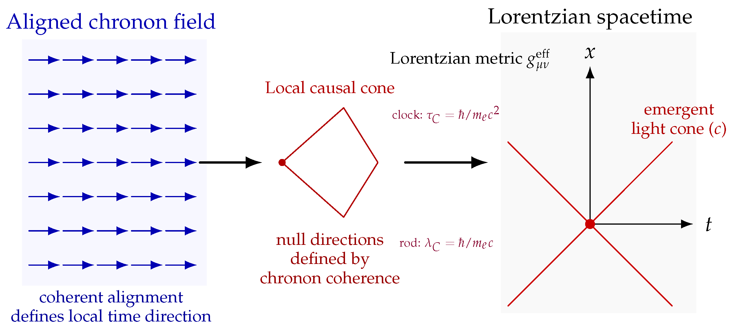
Figure 2.
The Real–Now–Front (RNF) as the generator of spacetime. Left: The aligned and fully geometric past, where chronon patterns are already fixed and no further evolution occurs. Center: The RNF slice , the unique locus where the chronon field is coherently aligned and where geometry, matter, and fields exist. Right: The pre-geometric reservoir , a non-metric collection of chronon microstates representing unrealized future degrees of freedom. As the RNF advances, it locally aligns microstates in and generates the next geometric slice, continually converting potential structure into realized spacetime.
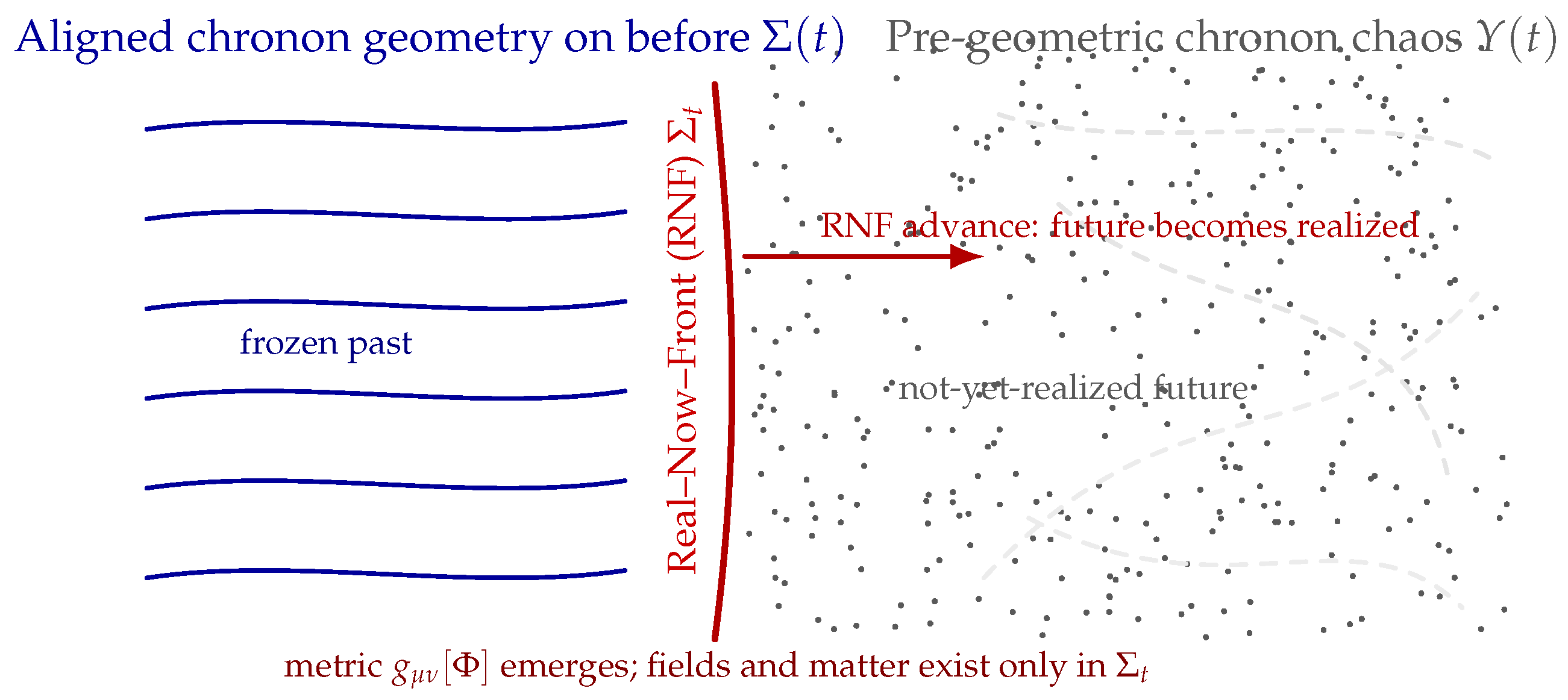
Figure 3.
Compactification of action into a periodic manifold. A finite action quantum identifies S with , converting the real line of action into a sequence of equivalent phase circles. Each trajectory acquires a phase . Interference arises from the cyclic geometry of these phases.
Figure 3.
Compactification of action into a periodic manifold. A finite action quantum identifies S with , converting the real line of action into a sequence of equivalent phase circles. Each trajectory acquires a phase . Interference arises from the cyclic geometry of these phases.
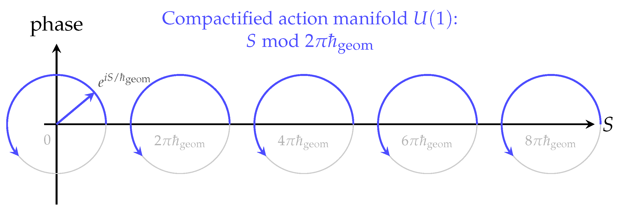
Figure 4.
Double–slit interference as modular phase geometry. Each path contributes a phase . The interference pattern on the screen results from the cyclic addition of these modular phases on the compact action manifold, without invoking an independent wave medium.
Figure 4.
Double–slit interference as modular phase geometry. Each path contributes a phase . The interference pattern on the screen results from the cyclic addition of these modular phases on the compact action manifold, without invoking an independent wave medium.
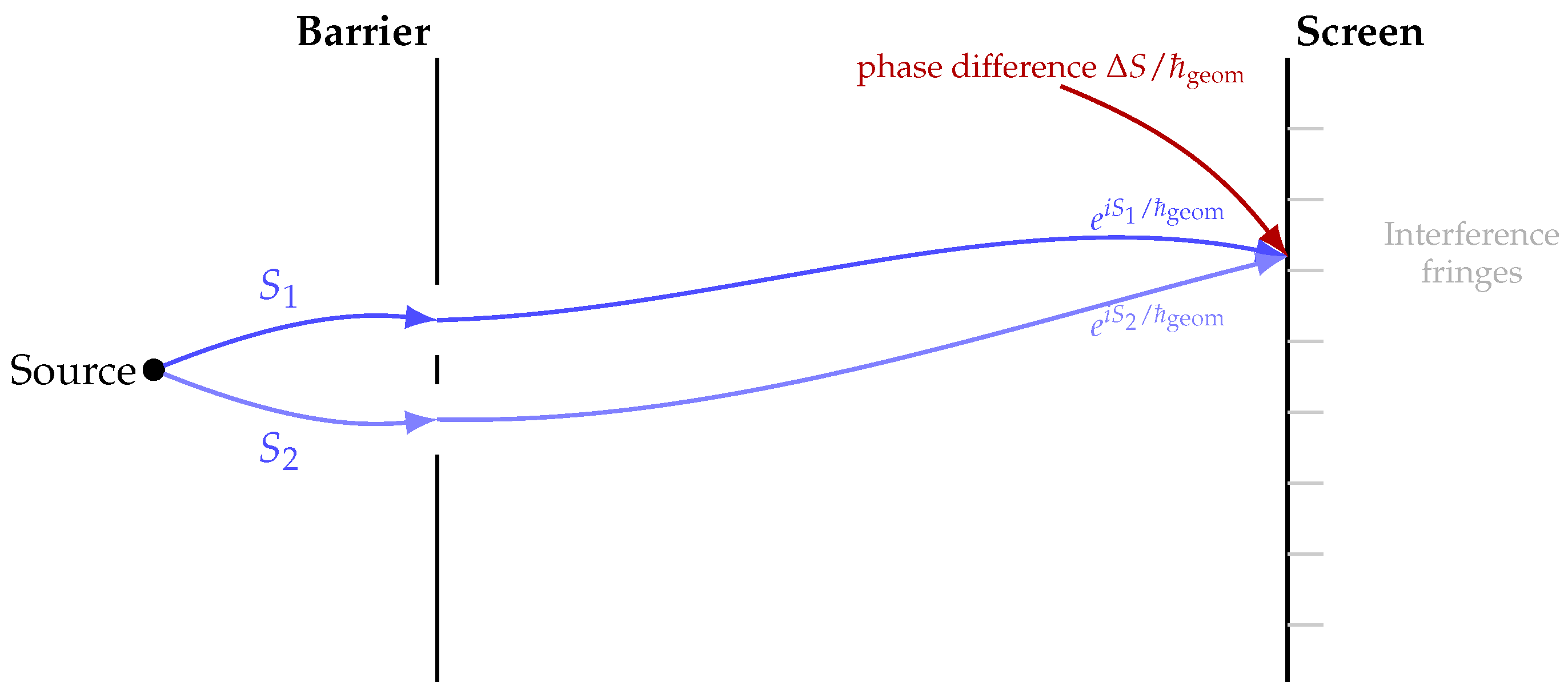
Figure 5.
Gauge Bridge in the Internal Chronon Bundle. Two solitons A and B reside in an aligned RNF slice . Their external DOFs (position, shape, metric data) form only local structures and, consistent with all known experiments, cannot be entangled. In contrast, their internal chronon DOFs (polarization, twist, compact-action phase) can support global compatibility constraints in the internal chronon bundle. A coherent internal-bundle pattern across the vacuum constitutes a gauge bridge, the physical origin of entanglement in RNF/ChFT. A local interaction at A disrupts internal alignment and destroys the global constraint, collapsing the entanglement.
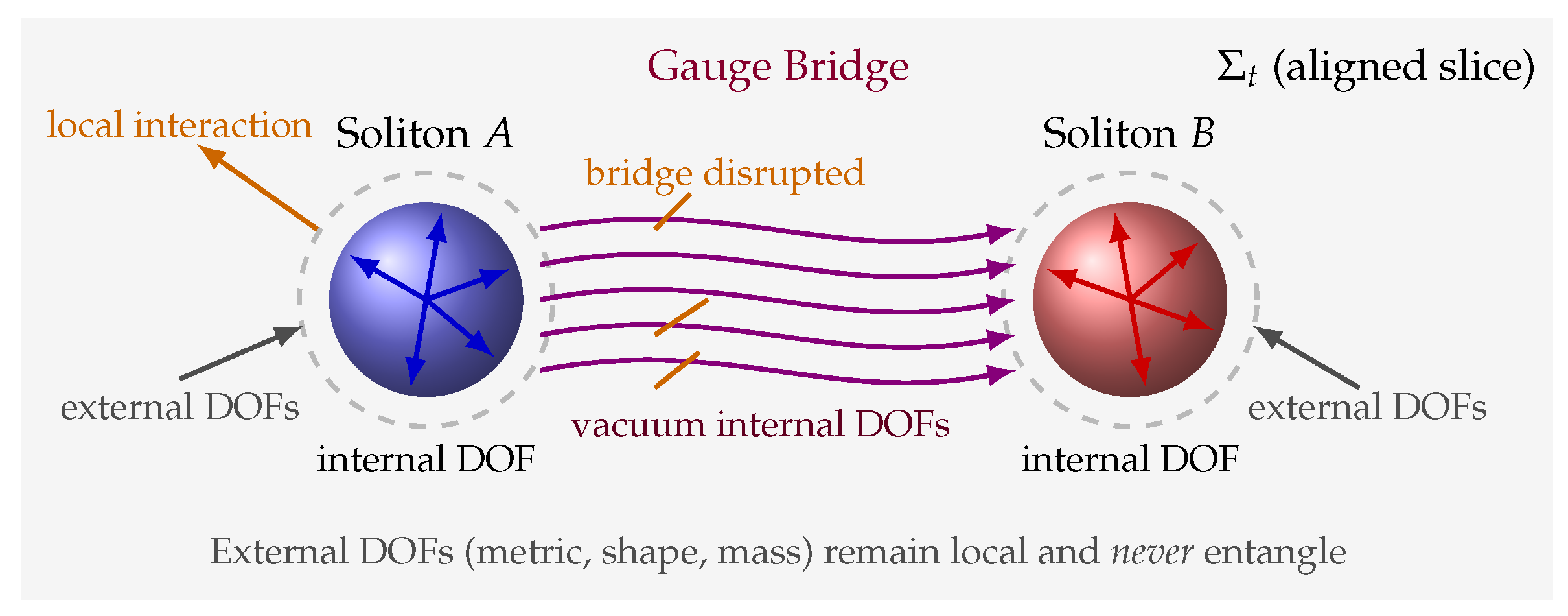
Figure 6.
Wave function visualization on an RNF slice . Each point carries two geometric indicators: (1) a blue “twist amplitude” arrow representing , and (2) a purple “phase direction” arrow encoding . A smooth phase gradient runs across the slice, and a shaded region illustrates locally enhanced amplitude. Together, these arrows depict the wave function as a twist–phase field intrinsic to the chronon medium.
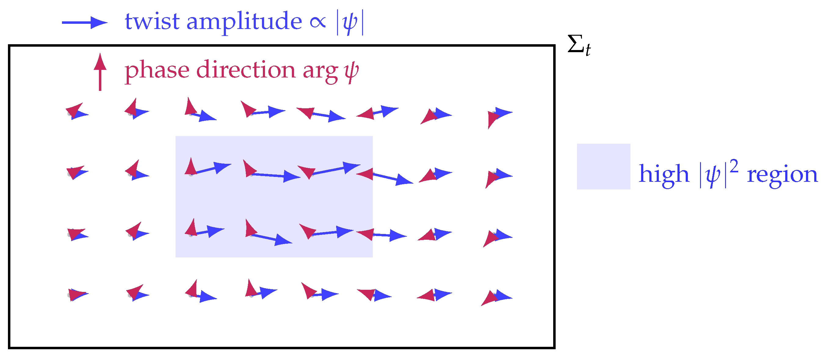
Figure 7.
RNF reconstruction preserves entanglement as a single joint constraint. Left: On the slice , the singlet condition is encoded directly in the aligned chronon pattern. Middle: As the RNF advances, reconstruction occurs locally and in parallel at all points, with no preferred update position and no need for nonlocal mediation. Right: On the next slice , the same constraint is restored automatically because it is part of the pattern that guides local alignment. Entanglement thus reflects the RNF’s simultaneous reconstruction of both spatial separation and the constraint linking the spins—not any within-slice signaling.
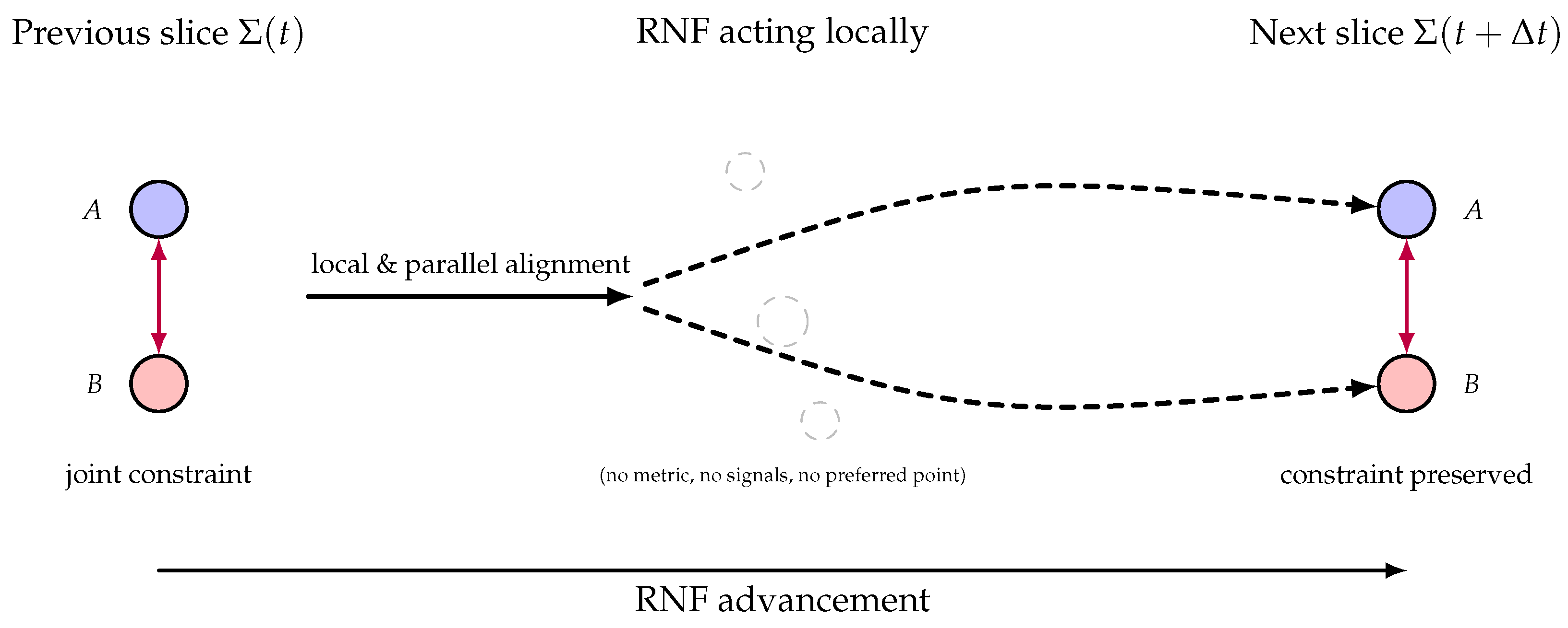
Figure 9.
Electron as the minimal chronon soliton. A single soliton carries (i) one unit of Abelian polarization flux (), (ii) an SU(2) double-cover holonomy giving spin , and (iii) a finite curvature energy that defines its mass . All three quantum numbers arise as geometric invariants of the same topologically protected soliton.
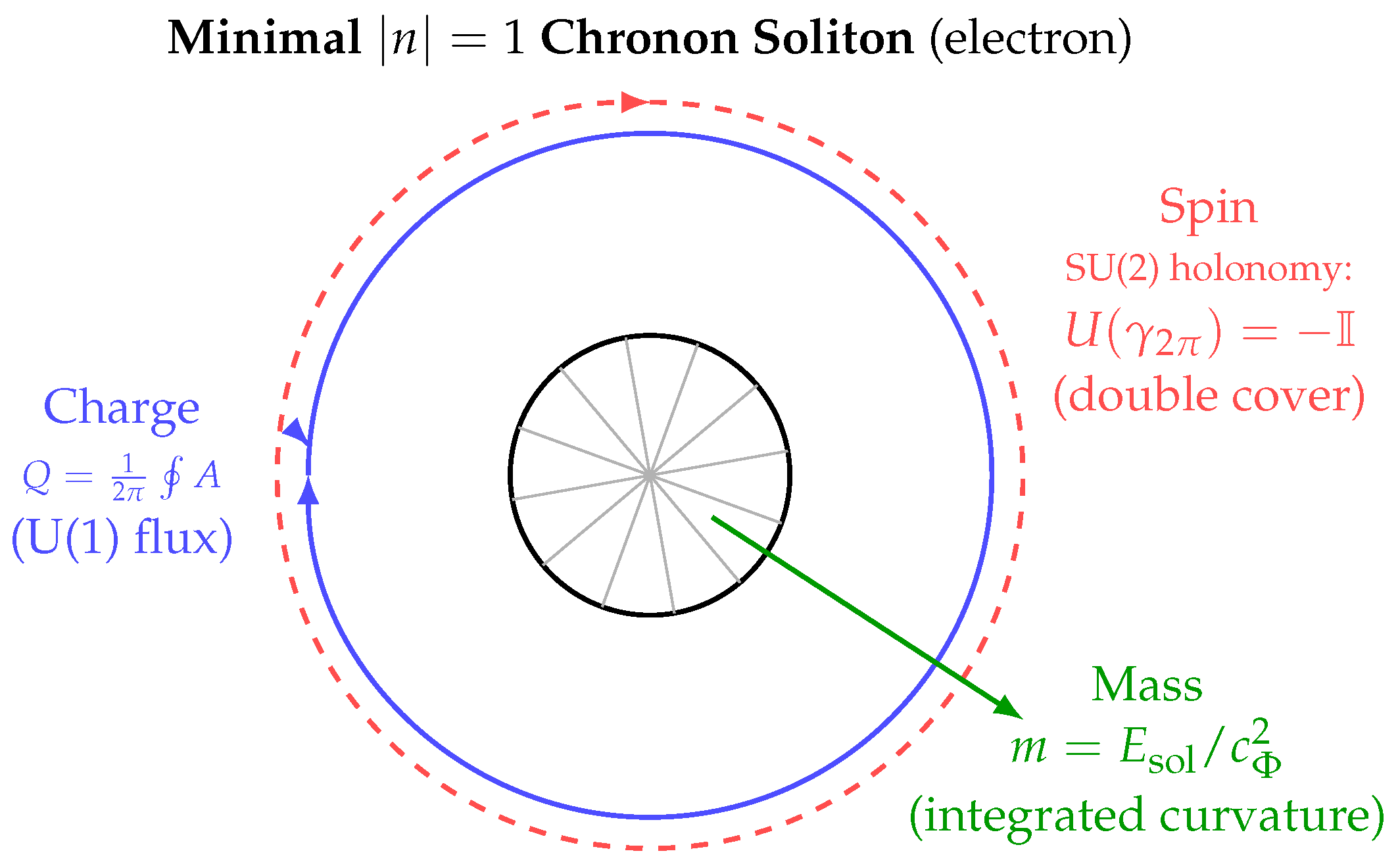
Disclaimer/Publisher’s Note: The statements, opinions and data contained in all publications are solely those of the individual author(s) and contributor(s) and not of MDPI and/or the editor(s). MDPI and/or the editor(s) disclaim responsibility for any injury to people or property resulting from any ideas, methods, instructions or products referred to in the content. |
© 2025 by the authors. Licensee MDPI, Basel, Switzerland. This article is an open access article distributed under the terms and conditions of the Creative Commons Attribution (CC BY) license (http://creativecommons.org/licenses/by/4.0/).
Copyright: This open access article is published under a Creative Commons CC BY 4.0 license, which permit the free download, distribution, and reuse, provided that the author and preprint are cited in any reuse.


