
Submitted:
01 December 2025
Posted:
02 December 2025
You are already at the latest version
Abstract
Predictive maintenance (PdM) often fails to progress beyond pilot projects because machine-learning-based anomaly detection requires expert knowledge, extensive tun-ing, and labeled fault data. This paper presents an automated prototype that builds and evaluates multiple anomaly-detection models with minimal manual configura-tion. The prototype automates feature creation, model training, hyperparameter search, and ensemble construction, while allowing domain experts to control how anomaly alerts are triggered and how detected events are reviewed. Developed in a multi-year photovoltaic (PV) solar-farm case study, it targets operational anomalies such as sudden drops, underperformance periods, and abnormal drifts, using expert validation and synthetic benchmarks to shape and evaluate anomaly categories. Ex-periments on the real PV data, a synthetic PV benchmark, and a machine-temperature dataset from the Numenta Anomaly Benchmark show that no single model performs best across datasets. Instead, diverse base models and both rule-based and stacked en-sembles enable robust configurations tailored to different balances between missed faults and false alarms. Overall, the prototype offers a practical and accessible path toward PdM adoption by lowering technical barriers and providing a flexible anoma-ly-detection approach that can be retrained and transferred across industrial time-series datasets.
Keywords:
predictive maintenance
; time-series anomaly detection
; ensembles
; autoencoders
; one-class svm
; isolation forest
; time-aware metrics
1. Introduction
Predictive maintenance (PdM) aims to detect problems early and avoid unplanned downtime by acting before failures occur thus reducing maintenance costs [1]. However, many PdM initiatives do not progress beyond the pilot stage. One contributing factor is the complexity of configuring and maintaining machine-learning–based anomaly detection (AD) systems. Domain experts must select appropriate models, adjust numerous hyperparameters, and often provide labeled fault data, which is expensive and rarely available at scale [2]. As a result, many organizations struggle to turn PdM concepts into routine, reliable operations.
In earlier work [3], we examined the interpretability challenges associated with anomaly-detection models. We developed a human-in-the-loop labeling and visualization tool that helps experts understand model behavior, validate detected anomalies, and create realistic synthetic benchmarks for PdM scenarios. The results indicated that expert feedback and transparent visualizations help reduce the gap between analytical model outputs and practical maintenance decision-making.
In this paper, we shift the focus from interpretability to automation and accessibility. We present an automated prototype that builds, tunes, and evaluates multiple anomaly-detection ML models with minimal manual configuration. The prototype automatically generates time-series specific features, trains several unsupervised base models, explores a range of hyperparameters, and constructs both rule-based and stacked ensemble models. Domain experts retain control by defining the temporal context considered by the model and specifying the criteria under which deviations are flagged as anomalies. This design reduces the need for machine-learning expertise while keeping the key operational decisions with the domain experts.
The prototype was developed in the context of a multi-year photovoltaic (PV) solar-farm case study operated at FH CAMPUS 02. This installation provides real-world production data with daily and seasonal patterns, weather influences, and equipment-related disturbances, making it a realistic test bed for anomaly detection. Together with domain experts, we identified practically relevant anomaly types such as sudden power drops, extended underperformance periods, and irregular production days. Expert-validated labels and a synthetic PV benchmark derived from the real data were used to evaluate model performance, and train different model configurations and better understand the performance of underlying models. To assess transferability beyond the PV domain, we further applied the prototype to a publicly available machine-temperature dataset from the Numenta Anomaly Benchmark (NAB), which represents a different industrial context and labeling scheme.
Existing approaches to anomaly detection in PdM often focus on individual algorithms or narrow benchmark settings [4,5,6,7,8,9]. In practice, however, three issues remain insufficiently addressed. First, model configuration and selection are still largely manual. Engineers must choose between multiple methods and hyperparameter settings, even though performance varies strongly across datasets and operating conditions. Second, many automated or AutoML-style frameworks treat configuration as a purely technical optimization problem and do not expose the few high-level controls that matter operationally, such as how much recent history should be considered or how strict alert thresholds should be. Third, cross-domain reuse is rarely demonstrated: solutions validated on a single asset or dataset often do not show how they behave when retrained on data from other industrial systems with different label structures and anomaly characteristics.
This paper addresses these gaps by pursuing the following objectives:
- O1 – Automate anomaly-detection configuration for PdM time series. We design and implement a prototype that automatically generates time-series features, trains multiple unsupervised base models, performs hyperparameter and threshold search, and constructs ensemble configurations, with minimal manual tuning required from domain experts.
- O2 – Provide an expert-centred configuration interface. We structure the system so that domain experts mainly interact with a small number of intuitive settings, most notably the lag window and anomaly-score threshold, while the prototype handles model selection and detailed configuration in the background.
- O3 – Demonstrate applicability in a real PV solar-farm case study. We evaluate the prototype using expert-validated anomalies and expert-designed synthetic anomalies derived from multi-year PV production data, showing how it supports practical maintenance decisions.
- O4 – Assess robustness and transfer across datasets and domains. We analyze the behavior of base models and ensembles across three datasets; real PV, synthetic PV, and a machine-temperature dataset from the NAB benchmark, using both pointwise and time-aware evaluation metrics to reflect practical maintenance requirements
The results show that automated exploration of diverse base and ensemble models, combined with expert-controlled configuration, provides robust anomaly detection across the three datasets and lowers the skills barrier for PdM adoption.
2. Related Work
2.1. Practical Barriers to PdM Adoption
Predictive maintenance (PdM) aims to reduce unexpected failures and associated costs by identifying faults before they occur. [1]. However, in many organizations, PdM initiatives do not progress beyond pilot phases and fail to transition into routine operational practice.
First, there is a significant skills gap. Modern PdM projects work with heterogeneous sensor streams and complex model outputs. Interpreting these results often requires both machine-learning and domain expertise, which is not always available within organizations [2,10]. Second, the availability of labeled fault data is limited. True failures and faults are rare and carefully labeling them in historical data is expensive and error prone. This limits fully supervised PdM approaches and motivates unsupervised or weakly supervised strategies instead [11,12]. Third, variability in operational context complicates the reuse and transfer of PdM models. Assets, sensors, and operating conditions differ from site to site, so a model that works well in one context may perform poorly in another [4,12]. Finally, evaluating anomaly-detection performance in PdM introduces several practical challenges. In many PdM scenarios, anomalies are not single points but intervals of abnormal behavior. Labels can be imprecise and incomplete, and human reviewers do not always agree. Standard pointwise metrics may then give a misleading picture, which complicates the comparison and selection of methods.
Collectively, these factors contribute to the observation that many PdM projects remain limited in scope rather than evolving into robust, scalable operational systems.
2.2. Domain-Driven Model Performance and Selection
Recent comparative studies indicate that no single anomaly-detection method consistently performs best across all datasets or operating conditions. Large-scale evaluations of time-series anomaly detection methods report that performance depends strongly on the dataset, the type of anomalies, and the evaluation protocol [5,6,7,8]. In some manufacturing case studies, relatively simple statistical or distance-based approaches have matched or even outperformed more complex deep-learning models [7]. These findings suggest that model selection should be guided by dataset characteristics and domain requirements rather than fixed algorithmic preferences. Because labeled faults are scarce, several authors have proposed unsupervised model-selection strategies. Instead of comparing models on many labeled anomalies, candidate detectors are ranked using indirect signals such as how their reconstruction error behaves over time or how they respond to injected synthetic anomalies [12]. This enables comparison of detectors and filter out clearly unsuitable configurations even when only a few real faults are known. Since data distributions can drift over time, periodic re-evaluation and updating of the chosen models is also recommended [4]. Ensemble approaches have also emerged as an effective strategy for increasing robustness by combining diverse base models (detectors). Complementary detectors can capture patterns that individual models fail to identify and aggregated decisions can be more stable than any single output. Benchmarks such as the Numenta Anomaly Benchmark (NAB) and TSB-UAD, as well as critiques of existing benchmarks, also stress that interval labels, temporal tolerance, and domain shift must be taken seriously when comparing methods and selecting models for deployment [5].
2.3. Anomaly Detection Techniques in PdM
PdM anomaly detection methods can be grouped into supervised, semi-supervised, unsupervised, and ensemble-based approaches [9].
Supervised and Semi-Supervised. Supervised methods treat anomaly detection as a standard classification problem. Models such as support vector machines (SVMs) or random forests are trained on labeled examples of normal and fault conditions [9]. When enough of high-quality labels exist, these models can perform very well. In practice, however, fault labels are often scarce, incomplete, or biased toward only a few failure modes. Semi-supervised approaches address this by exploiting abundant normal data and only a few anomalies. They either train one-class models on normal behavior or create pseudo-labels to better use the large unlabeled segments [13].
Unsupervised. Given that labelled faults are rare, unsupervised detectors are widely used in PdM [11]. They do not require labeled anomalies and instead learn a model of normal operation. Common categories include:
- Statistical models, such as ARIMA or Gaussian models, that flag deviations from expected trends or variability [7].
- Clustering and distance-based methods, such as k-means, Gaussian Mixture Models (GMMs), or Mahalanobis distance, that identify points far from typical clusters [7].
- Isolation Forest, a tree-based method designed for high-dimensional settings that isolates unusual points via random splits [14].
- One-Class SVM, which learns a boundary around normal data and treats points outside this boundary as anomalies [7].
- Reconstruction-based methods, such as Autoencoders or PCA, which reconstruct normal behaviour and signal anomalies when reconstruction error becomes high [9].
These methods are well suited to PdM scenarios where large volumes of normal data exist, but fault labels are limited.
Ensembles. Ensemble methods combine the outputs of several detectors (underlying base models) so that their strengths can compensate for one another. Simple rule-based ensembles apply majority voting, union rules (an alert if any model fires), or weighted voting where more trusted detectors have greater influence [15]. Stacked ensembles train a meta-model such as logistic regression or random forest on the scores produced by base models. When labels are scarce, synthetic anomalies or transferred labels can be used to train such meta-models [12]. In many industrial studies, these ensemble strategies are reported to provide more reliable anomaly detection across varied conditions than individual models alone [15].
Our work is related to AutoML ideas in that it automates hyperparameter tuning and model selection, but it differs in several ways. First, it is tailored specifically to time-series anomaly detection in PdM, where temporal context and interval labels play a central role. Second, it embeds domain-expert input into the configuration process by allowing domain experts to control how much recent history the models consider and how strict alert thresholds should be, aspects that generic AutoML systems usually ignore. Third, it integrates time-aware evaluation metrics such as PATE and Time-Adjusted F1, which better reflect operational requirements in PdM than purely pointwise scores. In this sense, the prototype builds on AutoML principles but adapts them to the specific challenges of PdM adoption.
Taken together, prior work shows that anomaly-detection performance is highly dataset-dependent, that configuration remains largely manual or technically oriented, and that cross-domain PdM evaluations are limited. Our prototype addresses these gaps by automating multi-model configuration for PdM time series, exposing only a few domain-relevant controls, and evaluating behaviour across three datasets with time-aware metrics
3. Materials and Methods
This section outlines the development of the automated anomaly-detection prototype, its data-processing pipeline, and its approach to model construction and evaluation for predictive maintenance. The emphasis is placed on the system’s practical workflow rather than the mathematical details of individual algorithms.
The prototype was developed in collaboration with domain experts from a photovoltaic (PV) solar-farm installation. Their operational experience shaped how anomalies should be defined, which patterns are relevant in practice, and which configuration options need to remain under expert control. The PV dataset served as the primary development environment, while two additional datasets, a synthetic PV benchmark and a machine-temperature data were later used to test how the prototype behaves on data from other domains.
At a high level, the prototype operates through four stages. First, it prepares the input time series by cleaning the data and creating the historical context and other relevant features that models require. Second, it automatically trains a diverse set of anomaly-detection ML models without needing labeled faults. Third, it constructs several ensemble model variants that combine the strengths of individual models. Finally, all detected anomalies are visualized and reviewed using the expert labeling tool introduced in our earlier work.
The subsections below describe the datasets, selected models, labeling workflow, and tuning strategy in more detail. The goal is to show how the systematic and automated structure of the prototype allows it to be applied to different types of operational data with only minimal expert input.
3.1. Datasets
The prototype was developed and tested using three datasets that represent different levels of complexity and different industrial contexts. The main goal of using multiple datasets was to show that the prototype can be applied to more than one type of time-series data without major manual adjustments.
Real PV Solar-Farm Dataset (Primary Dataset).
The development of the prototype was based on a multi-year case study conducted on an operational photovoltaic (PV) solar farm. This dataset contains daily and seasonal fluctuations in energy production and includes several real anomalies confirmed by domain experts. These anomalies include sudden drops in output, periods of underperformance, and irregular production behavior caused by weather, equipment issues, or measurement errors. Because this dataset reflects real operational conditions, it served as the foundation for prototype design and for identifying practically relevant anomaly patterns.
Synthetic PV Benchmark.
To test the prototype under controlled conditions, we created a synthetic PV dataset. It was generated from real PV data so that the general patterns remained realistic. Domain experts then injected synthetic anomalies such as drops, drifts, or irregular fluctuations. This synthetic benchmark enables controlled evaluation with known ground truth and facilitates systematic comparison of models under identical conditions.
Machine-Temperature Dataset (Cross-Domain Test).
To examine how the prototype behaves outside the PV domain, we used a publicly available machine-temperature dataset from the Numenta Anomaly Benchmark (NAB). This dataset contains temperature measurements recorded every five minutes over several months. The anomaly labels cover longer periods and represent developing faults in an industrial machine. This dataset enables an assessment of the automated model-building process on data with differing structures and anomaly characteristics.
Together, these three datasets provide a mix of real-world, synthetic, and cross-domain scenarios that allow the prototype to be evaluated in a comprehensive and realistic way.
3.2. Selected Models and Ensemble Strategies
The prototype includes several anomaly-detection models that were chosen to cover different types of behavior observed in the PV case study and in the additional datasets. Comparative studies in time-series anomaly detection show that no single method consistently performs best and that performance is strongly dependent on the dataset and application domain [5,6,8]. This motivates a design in which multiple models are trained and compared automatically. Rather than relying on manual model selection, the prototype evaluates all supported models and their combinations, so that domain experts can benefit from this diversity without needing machine-learning expertise. The overall architecture was chosen to balance three goals: (i) cover a broad range of anomaly types, (ii) keep configuration simple for domain experts, and (iii) support automated search over model families and hyperparameters.
We assembled a heterogeneous set of base models to span both traditional machine-learning and deep-learning paradigms. Boundary-based and tree-based methods provide lightweight detectors for compact normal behavior and clear outliers, while neural models capture more complex temporal patterns:
- One-Class SVM (OCSVM): Learns what “normal” looks like by creating a boundary around normal operating patterns. It is useful when normal behavior is clearly defined and anomalies appear as deviations from this boundary.
- Isolation Forest: Tree-based ensemble for unsupervised anomaly detection effective on both univariate and multivariate data. Detects unusual points by isolating them in a series of random splits. It works well for identifying sudden drops or spikes that stand out from the rest of the time series, which commonly occurred in the PV case study [14].
- Autoencoder (AE): Neural networks that reconstruct recent time-series behavior and flag anomalies when reconstruction error becomes unusually high. They are helpful for patterns where the curve shape matters, for example, gradual performance drifts or irregular production days in the PV farm. Variants such as feed-forward, CNN, LSTM, and hybrid forms are tested automatically [16].
- LSTM Prediction Model: Predicts the next data point and compares it with the actual value; large deviations indicate potential anomalies. It is particularly useful where sequential dependencies carry important information, such as temperature changes in the machine dataset [17].
During early experiments, LSTM prediction models with different window sizes and network settings were part of the candidate pool. However, under the available data and evaluation protocol they performed less competitively than the Autoencoder variants and the tree-based detectors. They were therefore excluded from the final set of models reported in the results, whereas CNN–LSTM Autoencoders remained in the prototype because they offered a good trade-off between flexibility and performance (see Section 5.1).
Because each model captures different anomaly types and prior work shows that their strengths vary across datasets, the prototype also builds ensemble models that combine multiple base model detectors. This increases robustness and helps the system perform well across datasets.
- Manual ensemble: Combine model outputs using simple rules: majority vote (anomaly when most models agree), union vote (anomaly if any model fires, for maximum coverage), or weighted vote (models contribute according to their reliability).
- Stacked ensemble: Use a small meta-model (such as Logistic Regression, Random Forest, or XGBoost) that learns how to combine the scores of the base models. The prototype trains this meta-model automatically using labels from the PV case study and the synthetic benchmark.
Manual ensembles aggregate model outputs on the fly, while stacked ensembles are pre-trained for deployment (Figure 1). After comparing all configurations, the prototype selects one model as the primary choice for productive use, based on the domain expert’s preferences for precision, recall, and F1. This selected model can be either a single base detector or one of the ensemble configurations, so that users deploy one clear solution in the operational system while still benefiting from the diversity explored during training. Together, the combination of diverse base models and straightforward ensemble strategies underpins the prototype’s behavior across the PV and machine-temperature datasets
3.3. Anomaly Labeling Process
The prototype relies on unsupervised models that learn normal behavior from historical data. These models do not require anomaly labels during training. However, reliable labels are still essential for three tasks: (i) evaluating how well different models and ensembles perform, (ii) training stacked ensembles that learn how to combine model outputs, and (iii) visually checking whether detected anomalies are meaningful from an operational perspective.
For the PV case study, anomaly labels were created in close collaboration with domain experts using the web-based labeling tool introduced in our previous work. The tool displays the time series together with model scores and allows experts to interactively mark intervals as anomalous. During several labeling sessions, experts identified real events such as sudden production drops, longer underperformance periods, and irregular days caused by shading, weather, or equipment issues. These sessions contributed to refining the anomaly categories that are relevant for the PV system.
In addition to real events, we constructed a synthetic PV benchmark. First, a new synthetic time series was generated based on the original PV dataset so that its daily and seasonal patterns remained realistic. On top of this synthetic baseline, domain experts then used the labeling tool to inject artificial anomalies such as abrupt drops, gradual drifts, and abnormal fluctuations (Figure 2). All injected anomalies had to remain physically plausible (for example, no negative power values and realistic durations and magnitudes). This procedure increased the variety of anomaly patterns while keeping the data realistic, and it provided a controlled setting with known ground truth for comparing models and ensemble strategies.
For the machine-temperature dataset from the Numenta Anomaly Benchmark, we used the provided labels without modification. The labeling tool was applied here mainly for visualization and qualitative review. Domain experts can inspect how detected anomalies align with labeled intervals and where the prototype flags early-warning signals that fall slightly outside the official intervals. This helps to interpret quantitative results and understand model behavior in a different industrial domain.
Overall, the anomaly labeling process combines real case-study annotations, expert-designed synthetic anomalies, and existing benchmark labels. It provides the ground truth needed to compare models, train stacked ensembles where appropriate and verify that the prototype’s detections are meaningful in practical maintenance settings.
3.4. Configurable Variables and Tuning Parameters
The prototype distinguishes between configuration choices that domain experts actively influence and model-specific parameters that are handled automatically. This reflects the overall goal of simplifying model configuration for domain experts. Experts work mainly with a small number of intuitive settings, while the prototype explores a larger configuration space in the background.
Dataset-Specific Configuration (expert-facing settings)
For each dataset, the prototype exposes a limited set of configuration options that are meaningful from an operational point of view. The most important are the length of the lag window and the choice of anomaly-score threshold.
The lag window controls how much recent history the models see when assessing whether a point is anomalous. To identify reasonable ranges, we examined how strongly each time series depends on its recent past and then tested several candidate window sizes. For the PV dataset, this analysis and subsequent experiments suggested that small windows with a few past values (e.g., between 3- and 10-time steps) were sufficient to capture the most relevant dynamics without overfitting. Similar procedures were applied to the synthetic PV and machine-temperature datasets.
The anomaly-score threshold converts continuous model scores into binary decisions. In practice, this threshold represents a trade-off between false alarms and missed detections. The prototype uses quantile-based thresholds at the 80th, 85th, 90th, and 95th percentiles of the score distribution. Lower thresholds favor recall by flagging more events, while higher thresholds favor precision by raising alerts only for the most extreme scores. Domain experts can select an operating point that matches their cost structure, for example favoring high recall in safety-critical settings or higher precision when inspections are expensive.
To prevent regular daily or seasonal patterns from being misclassified as anomalies, the prototype also supports dynamic baselines and basic preprocessing. Moving averages and standard deviations over appropriate windows (for example, around one day of readings for the machine-temperature data) are used to normalize fluctuations [18]. Time-based features such as hour of day or day of year help the models recognize recurring patterns, and standardization ensures that all input features are on comparable scales. Missing values are handled through simple interpolation or forward filling so that the models receive continuous input series.
Model Hyperparameters (automatically tuned)
Once the dataset-level configuration is set, the prototype automatically explores hyperparameters for each base model and for the stacked ensembles. No manual tuning is required from the user. For each model family, we defined a small, literature-inspired grid over key parameters (e.g., ν and kernel type for One-Class SVM, number of trees and contamination rate for Isolation Forest, encoding dimensions and learning rates for Autoencoders, and regularization strength or tree depth for meta-models) [14,16,17]. In total, around 1300 different configurations were evaluated across all datasets. The complete hyperparameter grids for all base models and meta-models are reported in Table A1 and Table A2 (Appendix A).
During early experiments, the LSTM prediction models described above were included in the pool of candidates. Their performance turned out to be less competitive on the available data, and they were therefore not part of the final set of models discussed in the results. The impact of these architectural choices is addressed further in Section 5.1.
By separating expert-facing configuration from automatic hyperparameter search, the prototype keeps interaction simple while still performing a thorough and explicitly documented exploration of the space of possible models. This supports reproducibility while reducing manual trial-and-error and making advanced anomaly detection more accessible for predictive maintenance applications.
3.5. Prototype in the PV System Landscape
The anomaly-detection prototype was developed and deployed in the context of a photovoltaic (PV) solar farm operated at FH CAMPUS 02. This PV installation provides real production data and a realistic operational environment, making it the central case study of this work. In this setting, the prototype is not an isolated tool but one element of a broader system landscape that manages energy generation, data collection, analysis, and maintenance decisions. The overall PV system consists of four interconnected systems (Figure 3):
- System 1- Hardware infrastructure: solar panels, inverters, and control units for harvesting and distributing energy.
- System 2- Data collection and management: acquisition of measurements (e.g., panel output, inverter status, weather sensors) and central storage in a dedicated SQL-based data warehouse.
- System 3- Data Analysis and Visualization: web-based dashboards (Grafana, XAMControl) that allow domain experts to track performance and analyze data.
- System 4- Predictive system (this Prototype): the anomaly detection Prototype that automates model creation, configuration, and evaluation for predictive maintenance.
The prototype was designed in close collaboration with domain experts to fit into this landscape with minimal disruption. System 1 and System 2 provide the high-quality data required for model training and monitoring. System 4 consumes this data, performs automated model selection and evaluation, and produces anomaly scores and alerts. These outputs can then be inspected in the labeling and visualization tool and, where desired, linked back into System 3 dashboards to support routine maintenance workflows.
By situating the prototype within an existing PV system architecture, this section illustrates how the approach can be integrated into real industrial environments. For readers from industry, the four-system view offers a blueprint: starting from data acquisition and storage, the prototype can be added as an additional predictive layer that enhances existing monitoring with automated anomaly detection and expert-in-the-loop validation.
3.6. Reproducibility Capsule
To ensure reproducibility, experiments were conducted using an approximate chronological train–test split: about 85% of normal data for training and the remainder for testing. No separate validation set was used, as the priority was to give models the longest possible exposure to normal operating behavior. Base learners were trained with fixed random seeds (42) and repeated three times to assess stability. Typical runtimes were within minutes per dataset on commodity hardware (Intel ultra7 CPU, 32 GB RAM, no GPU). Hyperparameter search explored ~1,300 configurations automatically. Code and configuration scripts to reproduce the results, along with the synthetic PV dataset and references to the NAB dataset, are available at [https://github.com/dresanovic/anomaly-detection-framework].
4. Results
4.1. Evaluation Strategy
To obtain a comprehensive evaluation of the anomaly-detection methods, we employed a two-part protocol combining expert-driven qualitative review with quantitative performance measures.
Expert Review. For the PV case study, detected anomalies were first reviewed together with domain experts using the labeling and visualization tool. The tool overlays anomaly scores and binary detections on the original time series (Figure 4), enabling experts to determine whether flagged events correspond to sudden drops, extended underperformance periods, or other irregular patterns that are relevant for maintenance. This qualitative review helped identify clearly useful detections, borderline cases, and systematic failure modes (e.g., repeated false alarms during certain operating conditions).
Quantitative Metrics. To compare configurations systematically across datasets, we used standard classification metrics, Precision, Recall, and F1-score, based on anomaly labels from expert annotation (PV datasets), synthetic injections, and the NAB benchmark.
In time-series anomaly detection, anomalous events often span intervals rather than manifesting as isolated points. Standard metrics evaluate each timestamp separately and can penalize predictions that are only slightly misaligned. To address this, we included time-aware metrics:
Point-Adjusted Time-Error (PATE): Marks a detection as valid if it occurs anywhere inside a labeled anomaly interval, reducing penalties for slight temporal misalignments [19].
Time-Adjusted F1 (TimeAdj): Credits detections that fall within a small tolerance Δ near the boundary of labeled anomalies, making evaluation more realistic in maintenance contexts.
Labeling Tool and Synthetic Stress Testing. Our web-based tool (Figure 2) accelerated annotation and validation, while artificial anomaly injection allowed controlled tests to probe model strengths and weaknesses.
For each data set, base and ensemble models were evaluated under the same protocol, using the expert labels and synthetic anomalies described in Section 3.3. The combination of expert review and time-aware metrics aligns with the prototype’s goal of providing evaluation that reflects real maintenance needs rather than relying solely on idealized, point-level correctness.
4.2. Case Study Photovoltaic Dataset Results
For the PV case study, detections were first reviewed visually together with domain experts. Using the labeling and visualization tool, anomaly scores and binary flags were overlaid on the PV power curves (Figure 5 and Figure 6). This step verified that model-detected anomalies correspond to actual disturbances, indicating their operational relevance. Based on these expert-validated labels, we then compared base models and ensembles using the evaluation protocol from Section 4.1.
Table 1 summarizes representative configurations across varying lag settings and anomaly-score thresholds. Results show that stacked ensembles generally outperformed base models. The stacked Logistic Regression ensemble (lags 4–4–4, threshold at the 95th percentile reached an F1-score of approximately 89.3% with precision of 91.7% and recall of 87.1%. Stacked Random Forest and XGBoost ensembles also performed strongly, with F1-scores around 85.5%, driven by high recall (around 93%) and moderately lower precision (about 79%). Manual ensembles demonstrate how the prototype can support different operating policies. Majority and weighted voting schemes produced very high precision (up to 98.2%) but only moderate recall (around 57%), making them suitable when unnecessary inspections are particularly costly. In contrast, the union vote achieved recall above 94% at the expense of reduced precision (roughly 63–73%), prioritizing maximum anomaly coverage at the expense of an increased number of false positives.
Among base models, the Autoencoder (lag = 4) was the most effective with F1 ≈ 80.7% (P = 90.0%, R = 73.2%). Isolation Forest and One-Class SVM performed less reliably, with F1 ranging from 60–79%.
Overall, the experiments showed that intuitive guesses about “good” parameter settings were often wrong. Reliable configurations required a systematic search combined with feedback from domain experts. Which model and threshold to use should ultimately reflect the priorities of the application, whether the aim is to avoid false alarms, capture as many anomalies as possible, or strike a balanced approach with F1-score. The observed advantages of stacked and manual ensembles are consistent with earlier work indicating that ensemble and hybrid strategies tend to be more robust in complex PdM scenarios.
4.3. Synthetic PV Dataset Results
The synthetic PV benchmark was designed to complement the real PV case study with a controlled yet realistic test bed. As described in Section 3.1, a new synthetic time series was generated based on the original PV data so that its daily and seasonal patterns remain realistic. Domain experts then used the labeling tool to inject artificial anomalies (e.g., abrupt drops, gradual drifts, abnormal fluctuations) under physical plausibility constraints. This configuration preserved the statistical structure of the PV series while providing a known ground truth for systematic comparison of models and ensemble strategies.
On this dataset, the Autoencoder emerged as the strongest base model. With a lag window of 4 and an anomaly-score threshold at the 85th percentile, it achieved an F1-score of 87.2% (precision 91.0%, recall 84.4%). Isolation Forest favored high precision (around 93%) but showed considerably lower recall (about 46%), making it suitable when missed anomalies are less critical than avoiding false alarms.
Ensemble models confirmed the benefits of combining detectors. A stacked XGBoost ensemble reached an F1-score of approximately 84.9% (precision 93.0%, recall 78.0%), offering a balanced trade-off between precision and recall (Figure 7). Conversely, a precision-tuned stacked Logistic Regression configuration achieved 100% precision but only 15% recall, resulting in an F1-score of 25.3%. This configuration demonstrates that ensembles can be tuned to prioritize either low false-positive rates or higher anomaly-capture rates, depending on maintenance priorities.
Overall, the synthetic PV benchmark reinforced the complementary strengths of base and ensemble models observed in the real PV case study. Autoencoders provide a strong default for balanced detection, Isolation Forest supports high-precision configurations, and stacked ensembles allow domain experts to adjust the precision–recall balance. These patterns support the broader conclusion that no single anomaly detector is universally optimal and that automated model and ensemble selection is necessary to obtain robust performance across operating conditions.
4.4. Machine Temperature (NAB) Dataset Results
The machine-temperature dataset from the Numenta Anomaly Benchmark (NAB) was used to examine how well the prototype transfers to a different industrial domain. In contrast to the PV data, this series is more stationary and represents the gradual development of machine faults over time. Anomaly labels are provided as time intervals and were not modified. As in the PV experiments, the labeling and visualization tool was used primarily to inspect how model detections align with the labeled windows.
Visual inspection showed that the prototype detected all labeled anomaly intervals and often flagged early-warning signals shortly before the official start of a labeled period. These additional detections can be desirable in practice, because they highlight emerging problems earlier, but they are not counted as true positives under the strict benchmark protocol. Figure 8 shows the original anomaly labels, while Figure 9 illustrates the detections produced by our prototype.
Quantitatively, the best-performing configurations reached F1-scores of around 60–65%, with high precision and moderate recall. At first glance, the relatively low recall seems at odds with the visual impression that all labeled anomalies were detected and that some early-warning signals were even raised before the labeled periods.
The recall gap compared to visual assessments stems from the window-based labeling scheme of the NAB dataset. Anomalies are defined as continuous periods of roughly two days, often including non-anomalous segments, while detections are evaluated point by point. As a result, alarms that occur near but slightly outside the labeled window are counted as false negatives. This explains why recall values appear lower, even when the overall anomaly pattern was correctly identified. Time-aware metrics such as PATE and Time-Adjusted F1 alleviate, but do not entirely resolve, this mismatch by tolerating small temporal misalignments.
Overall, the NAB results indicate that the prototype can be transferred to a different domain with limited effort: all models are retrained on the new dataset, dataset-specific settings such as lag windows and thresholds are re-optimised, but the same set of base models and ensembles remain applicable. At the same time, the results underline the impact of labeling conventions and evaluation metrics when judging anomaly-detection performance across domains.
4.5. Summary of Experimental Results
Across the three datasets, the experiments show a consistent pattern. In the PV case study, stacked ensembles provided the most robust default performance, with the Logistic Regression ensemble achieving the highest overall F1-score. Manual ensembles offered interpretable operating modes: majority and weighted voting schemes delivered very high precision at the cost of reduced recall, while the union rule maximized anomaly coverage with more false alarms. Among base models, Autoencoders were the strongest individual performers, whereas Isolation Forest and One-Class SVM were more sensitive to configuration choices.
The synthetic PV benchmark confirmed and extended these findings in a controlled setting. Autoencoders provided a strong performance, Isolation Forest supported high-precision configurations, and stacked ensembles, particularly XGBoost, allowed the precision–recall trade-off to be tuned according to maintenance priorities. Because the synthetic anomalies were injected on top of a realistic PV baseline with known ground truth, this benchmark highlighted how different models specialize in different anomaly types and operating points.
On the machine-temperature dataset from the NAB benchmark, the same set of base models and ensembles remained applicable after retraining and re-optimizing dataset-specific parameters such as lag windows and thresholds. In this dataset, F1-scores were lower than in the PV experiments, primarily because of the window-based labeling scheme and pointwise evaluation, which penalize early warnings and detections near interval boundaries. Time-aware metrics and expert inspection indicated that many such detections retain operational relevance despite pointwise evaluation penalties.
Overall, the results indicate that no single anomaly detector is universally optimal and that combining diverse base models with automated search and ensemble strategies is essential for achieving robust performance across datasets. The next section discusses what drove these results and what they imply for the design and adoption of anomaly-detection solutions in predictive maintenance.
5. Discussion
5.1. What Drove Performance
Three factors most significantly influenced performance across the experiments: model diversity, ensemble strategies, and dataset-aware configuration. First, the prototype’s use of a heterogeneous set of base models contributed to robust performance. Tree-based methods such as Isolation Forest provided competitive baselines and were particularly effective at detecting sharp, isolated deviations. Autoencoders, especially the hybrid CNN–LSTM variants, were appropriate for modeling the daily and seasonal patterns of PV production as well as more complex disturbance patterns. LSTM prediction models were initially evaluated but showed lower performance under the available data and evaluation protocol and were consequently excluded from the final model pool.
Second, ensemble strategies played a key role in achieving robust performance. On the PV datasets, stacked ensembles consistently outperformed individual base models, while manual ensembles provided distinct precision- and recall-oriented configurations that domain experts can select according to their cost structure. The synthetic PV benchmark further illustrates how ensembles can be tuned from conservative, high-precision settings to more aggressive, high-recall configurations.
Third, dataset-aware configuration, in particular the choice of lag window and anomaly-score threshold, proved crucial. The experiments showed that intuitive expectations about “reasonable” parameter settings were often misleading. Effective configurations required a systematic search over lags, thresholds, and model hyperparameters, combined with feedback from domain experts. This is especially visible in the PV case study, where the best-performing configurations emerged from automated exploration rather than manual trial-and-error.
5.2. Implications for Predictive Maintenance Adoption
These findings carry several implications for the adoption of anomaly-detection solutions in predictive maintenance. Most importantly, the results reinforce that no single model is sufficient for all datasets or operating conditions. In practice, maintenance teams benefit from having a small set of deployable operating modes rather than a single universally optimal detector. The prototype addresses this by providing stacked ensembles as a robust default, together with manual ensembles that can be configured for high precision, high recall, or a balanced F1-score. This aligns with practical maintenance decision-making, as different assets or use cases may prioritize distinct trade-offs between false negatives and false positives.
The experiments also show that expert-in-the-loop workflows are essential. The labeling and visualization tool served two primary functions: it supported the creation and refinement of labels in the PV case study and synthetic benchmark, and it allowed experts to visually assess detections on the NAB dataset. This helped distinguish genuinely useful signals from artefacts and revealed early-warning detections that were not fully captured by pointwise metrics. Such tools are crucial for bridging the gap between model outputs and day-to-day operational decisions.
Finally, the cross-domain experiments on the machine-temperature dataset indicate that transfer to new domains is feasible with limited effort. All models are retrained on the new data, lag windows and thresholds are re-optimized, but the overall set of base models and ensemble strategies remains unchanged. This suggests that the prototype can serve as a reusable starting point for anomaly detection in other industrial settings, provided that appropriate labels or expert feedback are available for evaluation and threshold selection.
5.3. Design and Integration Considerations
From a design perspective, the prototype demonstrates how automation and simplicity can be combined in a single system. Internally, it performs a broad search over model families and hyperparameters; externally, domain experts mainly interact with a small number of intuitive controls. This separation allows domain experts to benefit from advanced model search without being exposed to its full complexity.
The PV case study also illustrates how such a prototype can be integrated into an existing system landscape. By connecting to the data warehouse of the PV installation, consuming time-series data from the monitoring systems, and feeding results back into dashboards and the labeling tool, the prototype acts as an additional predictive layer rather than a standalone application. This type of integration is important for adoption, because it avoids disrupting established processes and workflows.
In terms of computational overhead, training multiple models and ensembles is more expensive than maintaining a single detector. However, this cost is largely confined to the offline phase. Once a model configuration has been selected, interpreting new data is comparatively lightweight and can be performed on modest hardware. For many predictive maintenance scenarios, this trade-off is acceptable: it demands more computation during training but results in more robust and interpretable operating modes.
5.4. Contributions of This Work
To place the findings of this study into a broader context, this subsection summarizes the main contributions of the work. These contributions reflect both the methodological advances of the automated anomaly-detection prototype and the practical insights gained across the three datasets. Together, they outline how the proposed approach supports more accessible, consistent, and transferable predictive-maintenance workflows.
- 1.
- Automated anomaly-detection prototype: We introduce an automated prototype that trains, tunes, and compares multiple time-series anomaly-detection models, reducing the amount of manual machine-learning work required for PdM.
- 2.
- Expert-centered configuration: We design the system so that domain experts mainly interact with two intuitive settings: how much recent history the model considers when judging the current value (the lag window) and how high the alert threshold is. The prototype takes care of feature generation, model training, and ensemble construction.
- 3.
- Case study on a PV solar farm: We demonstrate the prototype in a real PV solar-farm setting, including expert-validated anomalies and expert-designed synthetic anomalies, and show how it supports practical maintenance decisions.
- 4.
- Evaluation across datasets: We test the prototype on real PV data, a synthetic PV benchmark, and a machine-temperature dataset from another domain. The experiments show that no single model is best everywhere and that different base and ensemble models become preferable depending on the data and the desired balance between missed faults and false alarms.
5.4. Limitations and Future Work
The study has several limitations that should be considered when interpreting the results and planning future work.
First, the number of datasets and domains is limited. Although the experiments cover a real PV installation, a synthetic PV benchmark, and a machine-temperature series from a public benchmark, many other asset types and failure modes were not considered. Additional case studies in different industries would be valuable for further stress-testing the prototype and extending its library of model families.
Second, the label quality and availability vary across datasets. In the PV case study, labels are based on expert judgment and synthetic injections, which, while realistic, may not capture the full range of possible anomalies. In the NAB dataset, the window-based labeling scheme leads to a mismatch with pointwise evaluation and affects recall. Future work could investigate alternative labeling schemes, semi-supervised approaches, or active learning strategies that reduce the annotation burden while improving label consistency.
Third, the current prototype focuses on batch-style training and evaluation. Models are retrained on historical data and then applied to new data in a static configuration. In real deployments, data distributions may drift over time, and asset behavior may change. Extending the prototype with incremental or periodic retraining, drift detection, and automated re-selection of operating modes would be a natural next step.
Finally, although the prototype already hides much of the ML complexity from end users, usability and explainability could be improved further. Future work could explore richer explanations for why a particular model configuration is recommended, as well as interactive interfaces that guide users through choosing operating modes based on their specific cost and risk constraints.
6. Conclusions
This work introduced an automated anomaly-detection prototype for predictive maintenance, developed within a photovoltaic (PV) solar-farm case study and evaluated across three datasets. The prototype integrates multiple base machine-learning models, both manual and stacked ensembles, and a web-based labeling and visualization tool that supports expert involvement. Its primary objective is to simplify the application of machine learning to time-series anomaly detection while providing flexible and robust operating configurations.
The experiments on the real PV case study indicated that stacked ensembles, in particular the Logistic Regression based ensemble, provided the most robust overall performance, while manual ensembles offered clear precision and recall oriented alternatives. Autoencoders demonstrated the highest performance among the individual base models, especially for capturing the daily and seasonal dynamics and disturbance patterns of PV production. The synthetic PV benchmark supported these findings under controlled conditions with known ground truth and highlighted how different models specialize in different anomaly types and operating points.
The machine temperature dataset from the Numenta Anomaly Benchmark demonstrated that the prototype can be transferred to a different industrial domain with limited effort. All models were retrained on the new data and dataset specific parameters such as lag windows and thresholds were re-optimized, while the overall set of base models and ensemble strategies remained unchanged. The results also underlined that labeling conventions and evaluation choices strongly influence reported performance, and that time-aware metrics such as PATE and Time-Adjusted F1 provide more realistic assessments when anomalies consist of intervals rather than isolated points.
Across all datasets, the study showed that no single machine-learning model is sufficient for all anomaly-detection scenarios. Instead, model diversity, ensemble strategies, and systematic configuration are needed to achieve robust behavior. The prototype addresses this by automating model and hyperparameter search internally, while exposing only a small number of intuitive controls to domain experts, in particular lag selection and alert thresholds. In combination with the labeling and visualization tool, this facilitates expert-in-the-loop workflows allowing detections to be inspected, validated, and refined.
Future work may extend these results in several directions, including additional industrial case studies, enhanced labeling strategies and active learning techniques, and support for incremental retraining and drift detection. Further developments in usability and explainability will also be important so that maintenance teams can better understand and trust the recommended models and operating modes. Overall, the prototype and corresponding findings contribute to the development of practical, automated, and expert-aware anomaly-detection solutions for predictive maintenance.
Author Contributions
Conceptualization, D.R. and N.B.; Methodology, D.R. and N.B.; Software, D.R.; Validation, D.R.; Formal analysis, D.R.; Investigation, D.R.; Resources, D.R.; Data curation, D.R.; Writing—original draft preparation, D.R.; Writing—review and editing, D.R. and N.B.; Visualization, D.R.; Supervision, N.B.; Project administration, D.R. and N.B.
Funding
This research received no external funding.
Institutional Review Board Statement
Institutional Review Board Statement: Not applicable.
Informed Consent Statement
Not applicable.
Data Availability Statement
The datasets used in this study include publicly available data as well as synthetic data generated for evaluation. All data are openly accessible in the GitHub repository Anomaly Detection Framework at https://github.com/dresanovic/anomaly-detection-framework/tree/main/notebooks/data.
Conflicts of Interest
The authors declare no conflicts of interest.
Appendix A Hyperparameter Grids and Configuration Details
This appendix provides detailed hyperparameter grids and dataset-specific configuration settings used by the anomaly-detection prototype. These details complement Section 3.4 and support reproducibility without interrupting the flow of the main text.
Appendix A.1 Base Model Hyperparameter Grids
Table A1 summarizes the hyperparameter ranges explored for the base anomaly-detection models.

Table A1.
Hyperparameter grids for base anomaly-detection models.
| Model | Hyperparameter | Values / Range |
|---|---|---|
| One-Class SVM | ν (nu) | {0.01, 0.05, 0.10, 0.50} |
| Kernel | {RBF, linear, polynomial, sigmoid} | |
| Gamma | {scale, auto} | |
| Isolation Forest | Number of trees | {100, 200, 300} |
| Max samples | {auto, 0.8} | |
| Contamination | {0.01, 0.02, 0.05} | |
| Max features | {1.0, 0.8} | |
| LSTM prediction | Units per layer | {32, 64} |
| Dropout | {0.2, 0.3} | |
| Training epochs | {30, 50, 70, 100} | |
| Batch size | {16, 32} | |
| Autoencoders | Encoding dimension | {4, 8, 12, 16} |
| (FF / CNN / LSTM / | Activation function | {ReLU, tanh, sigmoid} |
| hybrid variants) | Learning rate | {0.001, 0.0001, 0.00001} |
| Variant | {Feed-forward, CNN-based, LSTM-based, CNN–LSTM} |
Appendix A.2 Stacked Ensemble Meta-Model Grids
Table A2 summarizes the grids used for meta-models in stacked ensembles
Table A2.
Hyperparameter grids for meta-models in stacked ensembles.
| Meta-Model | Hyperparameter | Values / Range |
|---|---|---|
| Logistic Regression | Regularization C | {0.01, 0.10, 1.0, 10.0} |
| Random Forest | Number of trees | {50, 100, 200} |
| Max depth | {None, 5, 10} | |
| Max features | {sqrt, log2} (or default if library-specific) | |
| XGBoost | Number of trees | {50, 100, 200} |
| Max depth | {3, 5, 7} | |
| Learning rate | {0.01, 0.05, 0.10, 0.20} |
References
- Softic, S.; Hrnjica, B. Case Studies of Survival Analysis for Predictive Maintenance in Manufacturing. International Journal of Industrial Engineering and Management 2024, 15, 320–337. [Google Scholar] [CrossRef]
- Meyer Zu Wickern, V. Challenges and Reliability of Predictive Maintenance. Research Thesis, Rhein-Waal University of Applied Sciences, Faculty of Communication and Environment: Kleve, Germany, 2019. [Google Scholar]
- Resanovic, D.; Softic, S.; Balc, N. Explainable Anomaly Detection for Predictive Maintenance Using Synthetic Benchmarks and Human-in-the-Loop Labeling. In Proceedings of the Advances in Production Management Systems. Cyber-Physical-Human Production Systems: Human-AI Collaboration and Beyond; Mizuyama, H., Morinaga, E., Nonaka, T., Kaihara, T., von Cieminski, G., Romero, D., Eds.; Springer Nature Switzerland: Cham, 2026; pp. 89–103. [Google Scholar]
- Paparrizos, J.; Kang, Y.; Boniol, P.; Tsay, R.S.; Palpanas, T.; Franklin, M.J. TSB-UAD: An End-to-End Benchmark Suite for Univariate Time-Series Anomaly Detection. Proceedings of the VLDB Endowment 2022, 15, 1697–1711. [Google Scholar] [CrossRef]
- Wu, R.; Keogh, E.J. Current Time Series Anomaly Detection Benchmarks Are Flawed and Are Creating the Illusion of Progress (Extended Abstract). In Proceedings of the 2022 IEEE 38th International Conference on Data Engineering (ICDE); 2022; pp. 1479–1480. [Google Scholar]
- Schmidl, S.; Wenig, P.; Papenbrock, T. Anomaly Detection in Time Series: A Comprehensive Evaluation. Proceedings of the VLDB Endowment 2022, 15, 1779–1797. [Google Scholar] [CrossRef]
- Singh, K. Anomaly Detection and Diagnosis In Manufacturing Systems: A Comparative Study Of Statistical, Machine Learning And Deep Learning Techniques. In Proceedings of the Annual Conference of the PHM Society; September 2019; Vol. 11.
- Lee, S.; Kareem, A.B.; Hur, J.-W. A Comparative Study of Deep-Learning Autoencoders (DLAEs) for Vibration Anomaly Detection in Manufacturing Equipment. Electronics 2024, 13. [Google Scholar] [CrossRef]
- Barrish, D.; Vuuren, J. A Taxonomy of Univariate Anomaly Detection Algorithms for Predictive Maintenance. South African Journal of Industrial Engineering 2023, 34, 28–42. [Google Scholar] [CrossRef]
- Hrnjica, B.; Softic, S. Explainable AI in Manufacturing: A Predictive Maintenance Case Study. In Proceedings of the IFIP International Conference on Advances in Production Management Systems (APMS); Springer; 2020; pp. 66–73. [Google Scholar]
- Nota, G.; Nota, F.D.; Toro, A.; Nastasia, M. A Framework for Unsupervised Learning and Predictive Maintenance in Industry 4.0. International Journal of Industrial Engineering and Management 2024, 15, 304–319. [Google Scholar] [CrossRef]
- Goswami, M.; Challu, C.; Callot, L.; Minorics, L.; Kan, A. Unsupervised Model for Time-Series Anomaly Detection. In Proceedings of the ICLR; 2023.
- Potharaju, S.; Tirandasu, R.K.; Tambe, S.N.; Jadhav, D.B.; Kumar, D.A.; Amiripalli, S.S. A Two-Step Machine Learning Approach for Predictive Maintenance and Anomaly Detection in Environmental Sensor Systems. MethodsX 2025, 14, 103181. [Google Scholar] [CrossRef] [PubMed]
- Liu, F.T.; Ting, K.M.; Zhou, Z.-H. Isolation Forest. In Proceedings of the 2008 Eighth IEEE International Conference on Data Mining; 2008; pp. 413–422. [Google Scholar]
- Ao, D.; Gugaratshan, G.; Barthlow, D.; Miele, S.; Boundy, J.; Warren, J. An Ensemble Learning-Based Alert Trigger System for Predictive Maintenance of Assets with In-Situ Sensors.; September 2023.
- keras Timeseries Anomaly Detection Using an Autoencoder. Available online: https://keras.io/examples/timeseries/timeseries_anomaly_detection/ (accessed on 27 November 2025).
- Keras LSTM Layer. Available online: https://keras.io/api/layers/recurrent_layers/lstm/ (accessed on 27 November 2025).
- neptune.ai Anomaly Detection in Time Series 2023. 2023.
- Ghorbani, R.; Reinders, M.J.T.; Tax, D.M.J. PATE: Proximity-Aware Time Series Anomaly Evaluation 2024.
Figure 1.
Model repository and automated configuration workflow of the anomaly detection prototype. This diagram zooms into System 4 of the PV system landscape shown in Figure 3.
Figure 1.
Model repository and automated configuration workflow of the anomaly detection prototype. This diagram zooms into System 4 of the PV system landscape shown in Figure 3.
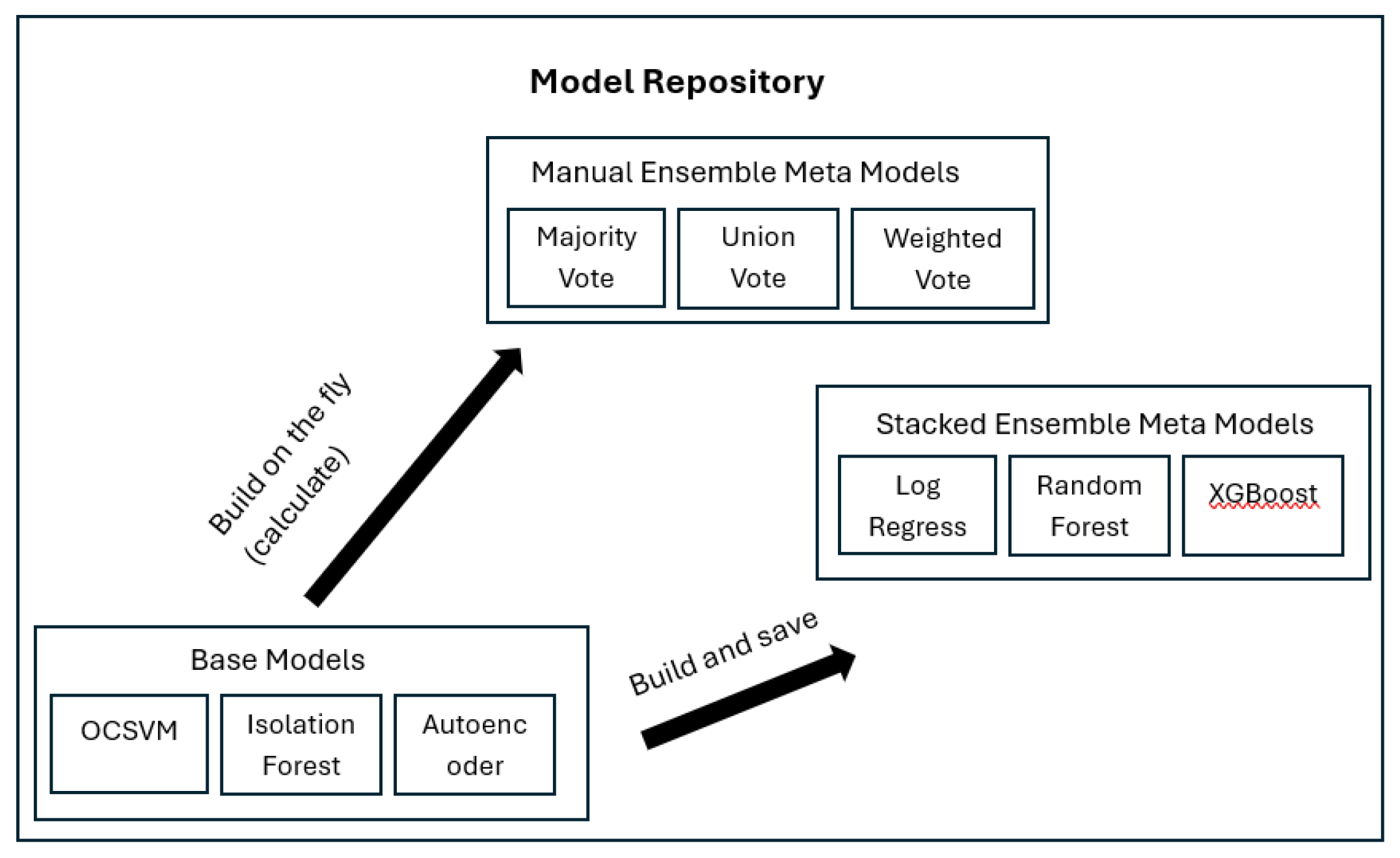
Figure 2.
Labeling tool with an example time-series and marked anomalies.
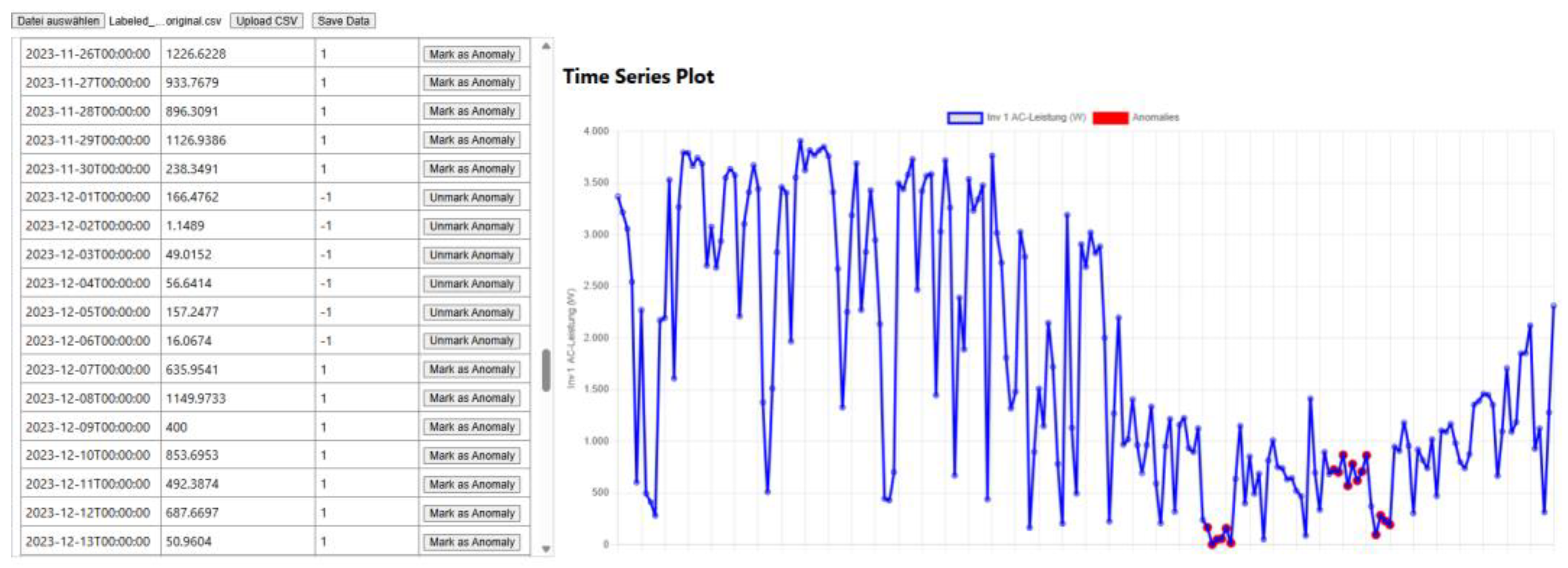
Figure 3.
PV system landscape with four interacting systems.
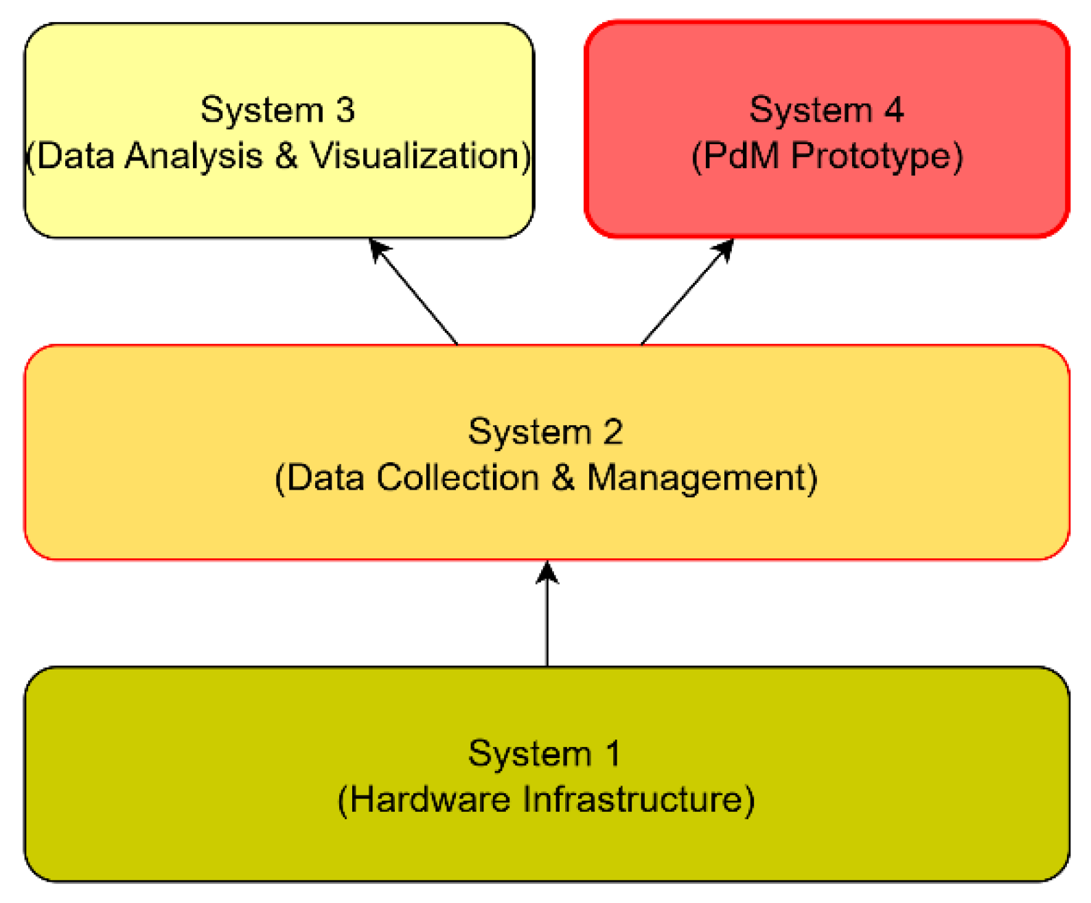
Figure 4.
Detected anomalies overlaid on PV output data.
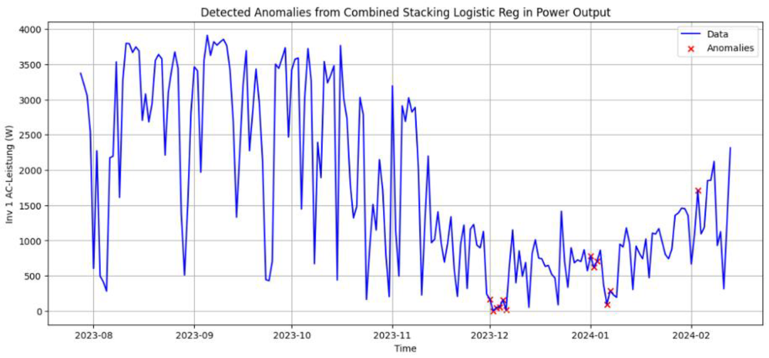
Figure 5.
Real anomalies labeled by expert domain.
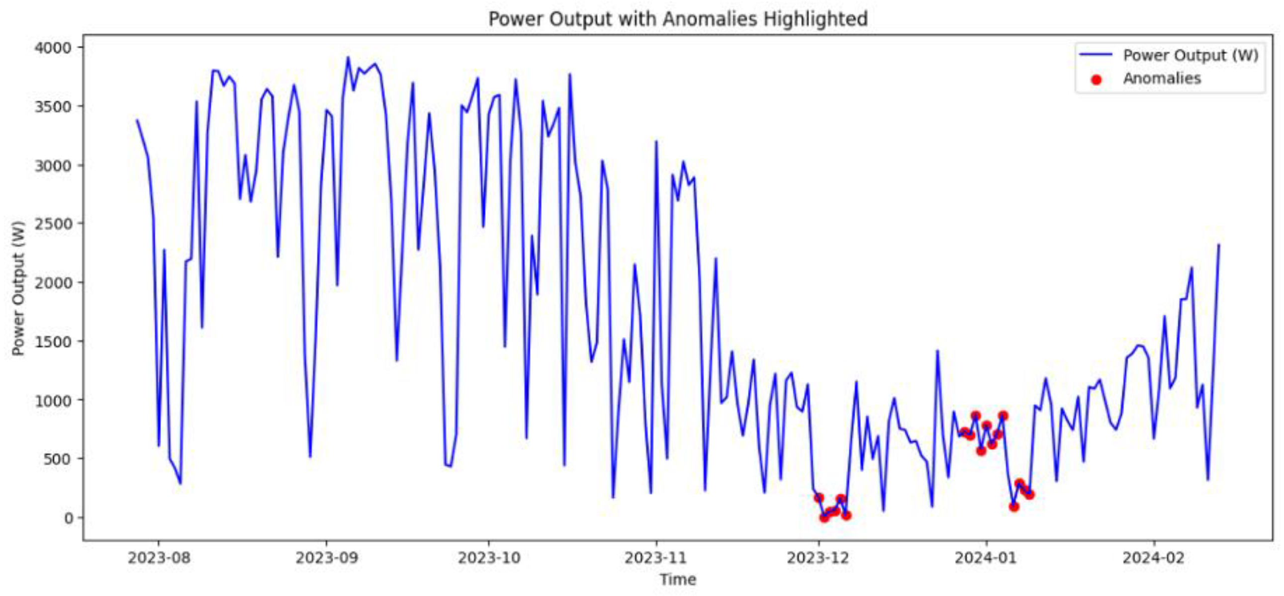
Figure 6.
Detected anomalies for a representative high-performing configuration.

Figure 7.
Expert-labeled (top) vs. detected (bottom) anomalies in synthetic PV dataset.
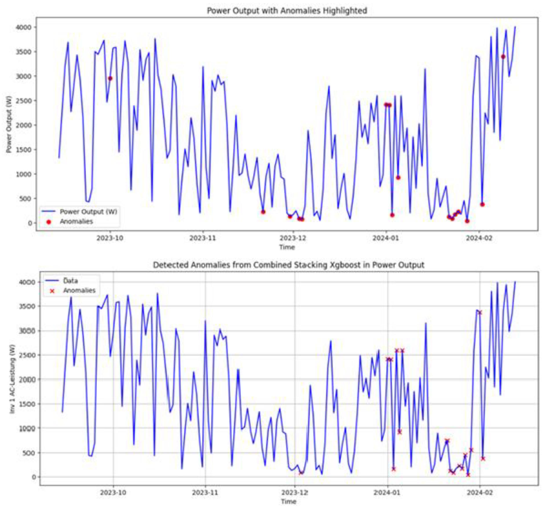
Figure 8.
NAB machine-temperature—labeled anomaly windows (visualization tool).
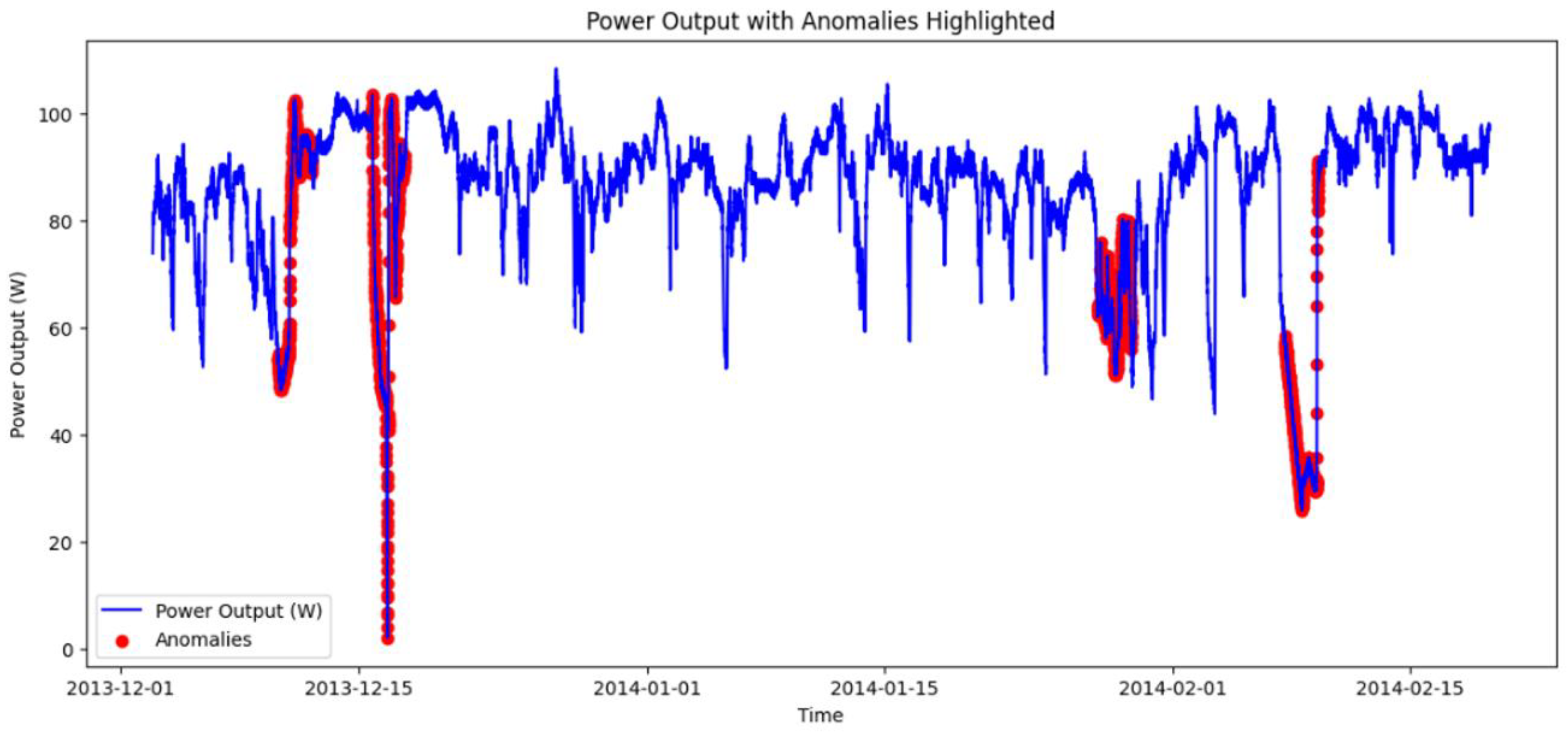
Figure 9.
NAB machine-temperature—detections produced by the framework.
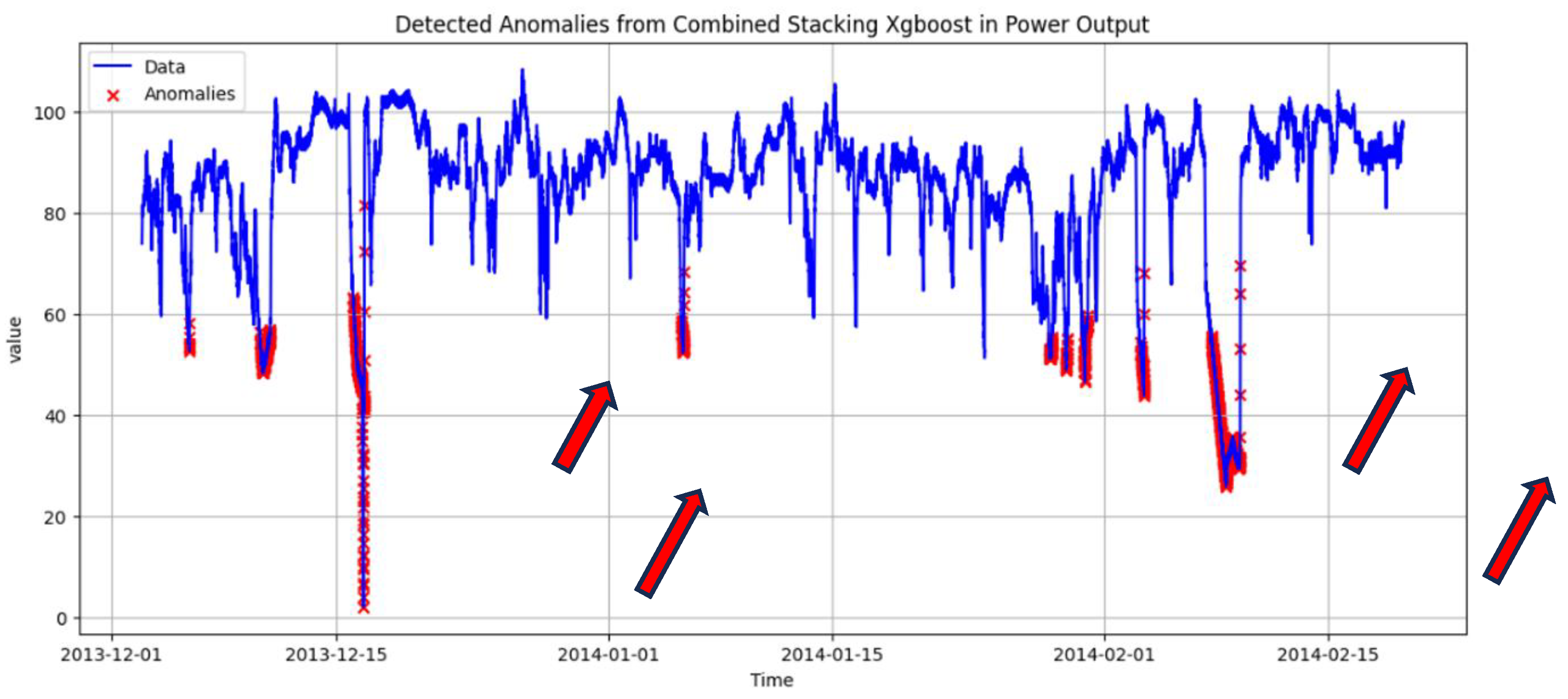
Table 1.
Representative model configurations for the PV solar-farm.
| Type | Model | Model Configuration | PATE (in Percent) | TimeAdj (in Percent) |
|---|---|---|---|---|
| Base Model | IsolationForest | Lag : 4 Threshold: p95 |
Precision: 74.3 Recall : 85.2 F1-Score : 79.4 |
Precision: 74.3 Recall : 80.1 F1-Score : 77.3 |
| Base Model | Autoencoder | Lag : 10 Threshold: p95 |
Precision: 88.4 Recall : 57.4 F1-Score : 69.6 |
Precision: 88.4 Recall : 57.4 F1-Score : 69.6 |
| Base Model | Autoencoder | Lag : 4 Threshold: p95 |
Precision: 90.0 Recall : 73.2 F1-Score : 80.7 |
Precision: 90.0 Recall : 76.3 F1-Score : 82.6 |
| Base Model | oc_svm | Lag : 4 Threshold: 95 |
Precision: 68.4 Recall : 54.7 F1-Score : 60.1 |
Precision: 68.4 Recall : 46.3 F1-Score : 55.2 |
| Ensemble Manual | union_vote | Lags : 4,10,4 Threshold: p95 |
Precision: 63.2 Recall : 89.9 F1-Score : 74.2 |
Precision: 63.2 Recall : 88.9 F1-Score : 73.9 |
| Ensemble Stacked | Logistic Regression | Lag : 4,10,4 Threshold: p95 |
Precision: 98.2 Recall : 57.4 F1-Score : 72.5 |
Precision: 98.2 Recall : 57.4 F1-Score : 72.5 |
| Ensemble Stacked | Random Forest | Lag : 4,10,4 Threshold: p95 |
Precision: 98.2 Recall : 57.4 F1-Score : 72.5 |
Precision: 98.2 Recall : 57.4 F1-Score : 72.5 |
| Ensemble Stacked | XGBoost | Lag : 4,10,4 Threshold: p95 |
Precision: 80.0 Recall : 89.8 F1-Score : 84.7 |
Precision: 80.0 Recall : 88.9 F1-Score : 84.2 |
| Ensemble Manual | majority_vote | Lag : 4,4,4 Threshold: p95 |
Precision: 87.5 Recall : 82.4 F1-Score : 85.0 |
Precision: 87.5 Recall : 72.2 F1-Score : 79.2 |
| Ensemble Manual | union_vote | Lag : 4,4,4 Threshold: p95 |
Precision: 72.8 Recall : 94.5 F1-Score : 82.2 |
Precision: 72.8 Recall : 94.5 F1-Score : 82.2 |
| Ensemble Manual | weighted_vote | Lag : 4,4,4 Threshold: p95 |
Precision: 87.5 Recall : 82.4 F1-Score : 84.9 |
Precision: 87.5 Recall : 72.2 F1-Score : 79.2 |
| Ensemble Stacked | Logistic Regression | Lag : 4,4,4 Threshold: p95 |
Precision: 91.7 Recall : 87.1 F1-Score : 89.3 |
Precision: 91.7 Recall : 77.8 F1-Score : 84.2 |
| Ensemble Stacked | Random Forest | Lag : 4,4,4 Threshold: p95 |
Precision: 78.7 Recall : 93.5 F1-Score : 85.5 |
Precision: 78.7 Recall : 92.6 F1-Score : 85.1 |
Disclaimer/Publisher’s Note: The statements, opinions and data contained in all publications are solely those of the individual author(s) and contributor(s) and not of MDPI and/or the editor(s). MDPI and/or the editor(s) disclaim responsibility for any injury to people or property resulting from any ideas, methods, instructions or products referred to in the content. |
© 2025 by the authors. Licensee MDPI, Basel, Switzerland. This article is an open access article distributed under the terms and conditions of the Creative Commons Attribution (CC BY) license (http://creativecommons.org/licenses/by/4.0/).
Copyright: This open access article is published under a Creative Commons CC BY 4.0 license, which permit the free download, distribution, and reuse, provided that the author and preprint are cited in any reuse.


