
Submitted:
28 November 2025
Posted:
28 November 2025
Read the latest preprint version here
Abstract
This study introduces an end-to-end framework for assessing the condition of road markings in high-resolution drone imagery by jointly localizing, classifying the type of road marking, and quantifying damage. Candidate markings are first detected with YOLOv9, enabling robust instance discovery across complex urban scenes. For fine delineation, detections from YOLOv9 are cropped and segmented by a standalone VGG16-UNet, which refines boundaries and object structures. Condition is then estimated at the pixel level by modeling appearance statistics with kernel density estimation (KDE) and Gaussian mixture modeling (GMM) to separate intact from distressed material. From these distributions, we derive a per-instance damage ratio summarizing the proportion of degraded pixels within each marking. All outputs are georeferenced to real-world coordinates, supporting map-based visualization and integration into road asset inventories. Experiments in unseen areas demonstrate consistent generalization, with performance reported using standard detection (precision, recall, mAP) and segmentation (IoU) metrics, alongside analyses of damage ratio stability and runtime. The results show that the proposed pipeline reliably identifies road markings, estimates their damage levels, and anchors findings in geographic space, offering actionable evidence for inspection prioritization and maintenance planning. Limitations and future work include broader category coverage, improved modeling under extreme lighting conditions, and cross-city validation.
Keywords:
road markings
; YOLO
; VGG16-UNet
; object detection
; semantic segmentation
; damage assessment
1. Introduction
Road markings are critical roadway assets; they provide lane guidance for drivers and serve as essential cues for advanced driver-assistance systems (ADAS) such as Lane Keeping Assistance (LKA). Field studies have shown that marking conditions and visibility influence detectability by LKA and relate to safety outcomes, underscoring the need for scalable and timely assessment of marking health [1]. Specialized retroreflectivity vans are labor-intensive, episodic, and difficult to scale across large networks, which can delay maintenance decisions and reduce the consistency of records [2].
Recent advances in high-resolution drone imaging and deep learning enable fine-grained analysis of linear pavement assets at the object level. In this work, we target three practical questions for road-marking management from drone imagery: Where is each marking (localization), what type of marking is it (categorization), and how deteriorated is it (damage quantification). Our pipeline exploits a modern one-stage detector, YOLOv9, to propose candidate markings, then performs pixel-accurate delineation using a VGG16-UNet segmentation model applied to detector-cropped patches (UNet originally introduced by Ronneberger [3]). To estimate the condition, we model appearance statistics within each segmented instance and separate intact from distressed material using kernel density estimation (KDE) and Gaussian mixture modeling (GMM). KDE has classical foundations in nonparametric density estimation [4,5], while mixture separation commonly relies on the Expectation Maximization (EM) algorithm [6]. We summarize per-object condition with a damage ratio, the proportion of pixels labeled as distressed within the marking, and georeference all outputs to real-world coordinates to support map-based visualization and integration with asset inventories.
The remainder of this article is organized as follows. Section 2 reviews related work on road marking detection, segmentation, and condition assessment. Section 3 presents the proposed method: Section 3.1 describes the datasets and annotation protocol; Section 3.2 outlines the end-to-end framework; Section 3.3 details road marking detection using YOLO; Section 3.4 describes the segmentation of detector crops; and Section 3.5 introduces damage estimation via KDE and GMM. Section 4 reports the experimental results. Meanwhile, Section 5 concludes with key findings and directions for future work.
2. Related Works
UAV and road scene imagery: UAV imagery has been leveraged to extract individual markings at centimeter-level geometry and to flag defective markings directly from photos, highlighting the promise of aerial surveys for network-scale inspection [7,8]. Street-view or vehicle platforms have also been used to build automated inspection systems that estimate a “damage ratio” after segmentation and inverse perspective mapping [9], but they are constrained by viewpoint and occlusion, motivating the complementary UAV use.
Object detection for road markings: One-stage detectors in the YOLO family dominate recent practice due to their speed and accuracy. YOLOv8, in particular, moves to an anchor-free head with modern training refinements and is a common starting point for marking or small-object detection in aerial scenes [7,10,11]. For UAV perspectives, improved YOLO variants have been tailored to markings and symbols, underscoring the utility of detector-first pipelines. In contrast, flight height (above 100 meters in urban areas) may reduce accuracy when segmenting directly compared to the sequential process of detection-segmentation.
Segmentation of markings (and available datasets, pixel-accurate delineation): It remains essential for measuring shape, width, and fine wear patterns. UNet is a widely adopted architecture for thin, high-contrast structures and remains competitive for road surface elements [12]. Beyond generic lane datasets, domain-specific corpora have emerged for symbolic road markings; the Road Marking Detection (RMD) dataset (Remote Sensing) provides more than 3 thousand pixel-labeled images across many classes and has catalyzed segmentation methods tuned to road graphics [12]. Other segmentation networks tailored to markings built on DeepLab-style encoders report strong mIoU on dedicated datasets, illustrating the benefits of context and attention for small, linear targets [13].
Condition and damage quantification: Image-based condition assessment typically segments markings and then estimates deterioration using geometric/photometric cues or projective normalization. Examples include hierarchical semantic segmentation with dynamic homography for objective damage scoring and street-view systems that compute the damage ratio after inverse perspective mapping (IPM) [9,14]. Probabilistic modeling offers a principled route to separate “intact” vs. “damaged.” appearances within a segmented instance (nonparametric KDE and GMM for partitioning heterogeneous pixel distributions) [5,6]. While deep learning semantic segmentation excels at multi-class damage categorization, in the binary setting of “damage” vs. “non-damage” pixels, our instance-wise probabilistic decision model achieves higher accuracy and yields more stable damage ratios.
Positioning of our work: Prior studies often address either detection or segmentation, or they quantify conditions at the regional level without per-instance, georeferenced outputs. Building on this literature, our study combines detector-guided cropping (YOLOv9) with VGG16-UNet segmentation and KDE/GMM–based pixel distribution separation to produce an interpretable per-object damage ratio and real-world coordinates suitable for asset inventories. References above demonstrate each ingredient separately; our contribution is to integrate them into a cohesive UAV-based pipeline and validate generalization in unseen areas.
3. Proposed Method
3.1. Datasets
Scope and acquisition: We use UAV images collected over urban road corridors under routine flight conditions. Each image carries georeferencing metadata to allow later projection of results to map coordinates. Permanent roadway markings constitute the label space; temporary construction items are excluded.
Annotation protocol: Labels are provided at two levels to support the two-stage pipeline: (1) instance-level bounding boxes with class IDs for RMD; and (2) pixel-accurate polygons delineating each marking for Road Marking Segmentation (RMS). Quality control included visual cross-checks and correction passes on ambiguous cases.
Data organization (matching Figure 1): Scenes are partitioned once at the image/scene level into Train (70%), Val (20%), and Unseen (10%) for RMD. The best detection model (selected on unseen IoU) is then applied to the full set to predict and crop detector-centered patches. These patches constitute the RMS dataset, which is split into Train (70%), Val (20%), Unseen (10%) for segmentation training and evaluation. The Unseen splits are held out for external generalization tests.
The strategic planning approach underscored a considerable emphasis on redundancy and elevated image resolution to facilitate robust photogrammetric processing. Comprehensive details regarding the flight configuration are delineated in Table 1.
To attain uniform radiometric integrity and spatial intricacy, a UAV-mounted camera with meticulously selected specifications was utilized. The sensor parameters employed during the image acquisition process are delineated in Table 2.
3.2. Proposed Framework
Figure 2 illustrates the proposed framework, consisting of three interconnected modules that process UAV images. This pipeline generates a per-object record, comprising the road-marking class, its georeferenced position (location), and a damage ratio derived from appearance statistics.
In this study, we present the development of an automated methodology for assessing the condition of road markings, leveraging scalable UAV imagery. The primary objective of this process is to accurately identify and quantify the damage ratio resulting from degradation, such as breakage, blurring, and general material deterioration. Ultimately, this enables the derivation of quantitative assessments for road marking defects from the analyzed data points. Our proposed system integrates a sophisticated framework encompassing detector-guided cropping, segmentation, and a novel application of statistical methods (KDE/GMM) for precise pixel-level damage quantification, yielding georeferenced outputs for asset management.
3.3. Road Marking Detection (RMD)
UAV surveys generate large image volumes with markings that are small, thin, and repetitive (arrows, crosswalk bars, turn symbols). A detector is needed to preserve recall on small/extreme-aspect objects, run fast enough for mission-scale processing, and produce stable class hypotheses for downstream segmentation and damage estimation. As a powerful model in the field of object detection, YOLO satisfies these requirements by casting detection as a single pass over the image, avoiding the proposal stage and delivering a favorable speed–accuracy trade-off for infrastructure mapping (original single-stage formulation in [15]). In our pipeline, YOLO provides reliable instance hypotheses that seed segmentation and photogrammetric georeferencing, so misses and false positives are minimized early, where they are most costly.
Figure 3.
YOLO detection model architecture.
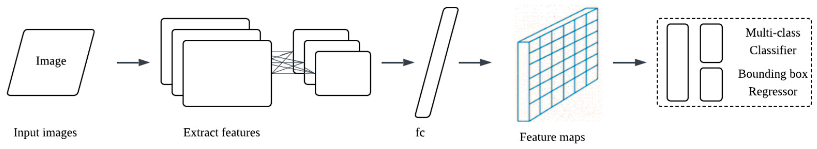
Feature extraction: A convolutional backbone computes multi-scale feature maps from the input image.
Prediction on a grid: A lightweight prediction head (represented as “fc” in the schematic) maps features to a dense grid. Implementation-wise, this is a stack of 1×1 and small k×k convolutions rather than a fully connected layer.
Outputs per cell: At each grid location, the head emits class logits and bounding box parameters relative to that cell/stride. Multi-scale heads (not drawn for clarity) ensure that both small and large markings are covered; this corresponds to the feature pyramid practice in contemporary YOLO designs [16,17].
Post-processing: Predictions from all scales are merged and filtered using non-maximum suppression to produce the final set of instances used by RMS and the damage module.
Task-specific advantages:
1. Sensitivity to thin structures. Dense, multi-scale predictions retain cues for strokes only a few pixels wide;
2. Aspect ratio flexibility. Modern, largely anchor-free heads avoid hand-tuned anchor shapes, improving boxes for elongated symbols. This trend follows anchor-free detectors, such as Fully Convolutional One-Stage Object Detection (FCOS) [17];
3. Throughput. One-stage inference enables tiling or batched processing for entire missions;
4. Clean interface. Each detection provides a class ID and a tight box; we pad the box with a small fixed margin before cropping for VGG16-UNet, which preserves full shapes for segmentation and stabilizes the later KDE/GMM decision.
Implementation notes: We train the detector on the split described in Figure 1, select the best checkpoint by validation (mAP50, mAP50-95 and F1) (Table 3) and use it to predict on all images. Margin-padded crops around each box form the inputs to the segmentation stage; centroids (or mask centroids later) are passed to the photogrammetric process for mapping.
3.4. Road Marking Segmentation (RMS)
RMS converts each detector-centered crop into a pixel-accurate, class-agnostic mask of the road marking. This mask preserves thin strokes and boundaries for geometric use and defines the support set for damage modeling, where KDE/GMM operates only within the predicted marking. In practice, high recall from RMD keeps true markings in the crop, while RMS provides the spatial precision that a bounding box cannot.
We used a UNet with a VGG16 encoder (pretrained) and a symmetric decoder. The encoder supplies four resolution stages of features; the decoder upsamples stepwise using transposed 2×2 convolutions. Skip connections reconcile high-level context with fine spatial detail crucial for narrow arrows and crosswalk bars. Each block in Figure 4 follows a lightweight recipe: Conv 3×3 + BN + ReLU, repeated twice, followed by downsampling (max-pool) in the encoder or upsampling in the decoder; the final 1×1 convolution with a sigmoid yields a probability map. UNet is a standard choice for the crisp delineation of thin structures [3], while VGG16 provides stable, well-understood features and benefits from large-scale pretraining [19].
- Skip connections and the shallow-kernel decoder preserve edges and narrow strokes that are easily lost in downsampling;
- VGG16’s pretrained filters accelerate convergence and help when the target appearance varies due to paint aging and surface texture;
- The model is compact, exportable, and decoupled from detection (RMD) proposes instances and IDs; RMS focuses solely on pixel-accurate shapes, keeping the pipeline modular and easy to maintain.
For each detection, the corresponding crop is forwarded through the network to produce a probability map. A threshold chosen on the validation set (applied uniformly at test time) converts probabilities into a binary mask. The mask centroid (or polygon) is passed to the photogrammetry module for georeferencing; the mask itself defines Mi for downstream KDE/GMM-based damage estimation.
3.5. Damage Estimation
We model the gray-level appearance of each detected road marking instance using a two-step statistical procedure. First, we obtain a smooth, nonparametric estimate of the gray-level distribution within the instance mask via KDE. Second, we approximate this KDE with a two-component GMM by maximizing a weighted log-likelihood on the intensity grid where the KDE is evaluated. The resulting mixture provides a compact, interpretable model of the apparent bimodality between intact (brighter) and distressed (darker) material, which we then use for pixel-wise Bayes classification and to compute a per-instance damage ratio. KDE follows the classical formulation of Rosenblatt and Parzen and the practical guidelines of Silverman [4,5,20]
In practice, we evaluate on a uniform grid (8-bit intensities). The bandwidth is set either by a fixed value (for reproducibility) or by a classical plug-in rule. This grid-based KDE stabilizes mode structure when the number of pixels per instance is modest and facilitates the subsequent weighted EM fitting.
Rather than fitting a GMM directly to raw pixels, we fit the mixture to the KDE so that the mixture curve adheres to the smoothed empirical density.
Let be the two-component mixture. On the grid , assign nonnegative weights (normalized so that ). We maximize the weighted log-likelihood using the EM algorithm [6]. With responsibilities
and the M step updates are:
This yields a mixture that closely tracks the KDE, including the inter-mode “valley” while retaining the interpretability and Bayesian decision rules of a parametric model.
- Bayesian pixel labeling and decision threshold
Let the darker component represent “damage” (configurable if illumination inverts the contrast). For a pixel of gray level , we assign the label with the larger posterior unnormalized score . The decision boundary solves the equality of posterior scores:
For a marking instance with pixel set and predicted labels , we report the damage ratio.
which summarizes the fraction of degraded material used in downstream mapping and inventory summaries.
3.6. Localization
We estimate absolute 3D coordinates of detected road markings (RM) by registering each incoming frame to a pre-built 3D reference model. The workflow comprises two parts:
- Reference model construction
SfM/MVS reconstruction: UAV multi-view imagery is processed with COLMAP to run structure-from-motion and multi-view stereo; features are detected and matched across images, and camera intrinsic/extrinsic parameters are estimated and globally refined by bundle adjustment; then, per-pixel parallax yields a dense RGB-D point cloud [21,22].
Outlier removal and database building: The cloud is denoised with statistical outlier removal (SOR) and radius outlier removal (ROR) to suppress artifacts from reflections, inter-image brightness differences, and texture heterogeneity [23]. The cleaned cloud, together with per-image features, per-pixel 3D coordinates, and camera parameters, is stored as a database used later for localization.
- 2.
- Assigning 3D coordinates to new detections
We carried out feature matching between input and reference images using SIFT [24], which is robust to rotation, scale, and illumination variations [25]. Each matched input pixel is linked to its corresponding 3D point in the reference model, giving absolute coordinates in the common frame.
For every detected RM, we select the five nearest matched points (Euclidean distance in the image domain) around the RM pixel and apply inverse distance weighting (IDW) to their 3D coordinates to obtain the RM’s absolute position [26]. Using five neighbors captures local depth/surface variation while avoiding over-smoothing; distance weighting stabilizes estimation on sloped or structurally varying pavement.
4. Results
4.1. Road Marking Detection Results
We trained and validated several YOLO families on the UAV-image split described earlier. For fairness, all detectors used the same input resolution and augmentation policy; confidence and IoU thresholds were tuned on the validation set and then fixed. Performance is summarized in Table 3 using Precision, Recall, F1, mAP50, mAP50–95, and computational cost (speed, GFLOPs). We emphasize F1 (the balance of misses and false alarms) and mAP50–95 (localization quality across IoU thresholds), because these criteria most strongly affect the downstream segmentation crops and, in turn, the reliability of damage estimation.
YOLOv8x offers balanced precision/recall but falls short of YOLOv9e in both F1 (92.984%) and mAP50-95 (64.256%).
YOLOv9e is the strongest overall detector for our pipeline. It delivers the highest F1 (93.642%) and the highest mAP50-95 (65.553%), while also achieving the top recall (91.982%) among the tested variants and maintaining a competitive runtime (0.8 ms/image; 189.2 GFLOPs). In a detector-first workflow, this combination is desirable: high recall reduces the number of markings that never reach segmentation, and high mAP50-95 indicates tighter boxes that yield better-centered, margin-padded crops for the segmentation model.
YOLOv10x attains the best mAP50 (95.803%) but lags in mAP50-95 (64.757%) and F1 (92.999%). The drop at higher IoU thresholds suggests slightly less stable localization, which can clip elongated arrows or crosswalk bars when crops are generated.
YOLOv11x shows the highest precision (95.556%) but lower recall (91.66%), implying more missed instances. In our setting, recall is critical; once a marking is missed, neither segmentation nor KDE/GMM can recover it.
YOLOv12x is close in F1 (93.454%) yet does not surpass YOLOv9e in the stricter mAP50-95 (64.749%) and is the heaviest among the high performers (1.3 ms/image; 198.6 GFLOPs).
The F1 improvements of YOLOv9e arise from a favorable trade-off: precision remains above 95% (95.363%) while recall increases to 91.982%. The mAP50-95 gain indicates that YOLOv9e retains quality as the IoU threshold tightens, which is consistent with more accurate box centers and extents. This matters practically because we expand detections by a fixed margin before cropping; better box geometry means fewer truncated symbols and less background in the crop, both of which simplify VGG16-UNet’s boundary tracing.
Visual inspection of false negatives shows that most misses occur on (1) very small or partially occluded markings and (2) symbols viewed under stronger obliquity. False positives are rare and typically involve high-contrast artifacts (e.g., manhole covers or pavement patches) that momentarily resemble arrows. Relative to other variants, YOLOv9e reduces both types: improved recall on small/thin elements lowers missed detections, and higher mAP50-95 corresponds to fewer loosely localized boxes that would otherwise crop in distracting backgrounds. These trends are consistent with the PR-curve shapes observed on the validation split (not shown for brevity) and hold when we apply the frozen model to the “unseen” scenes reserved for generalization checks.
Processing speed is adequate for mission-scale throughput. Although YOLOv10x is nominally faster in our measurements, YOLOv9e’s ~0.8 ms/image and moderate 189.2 GFLOPs keep GPU utilization manageable and allow dense tiling if needed. More importantly, the accuracy gains reduce error propagation to segmentation and damage estimation, which would otherwise incur greater downstream costs (extra post-processing, manual review, or re-flights).
Based on these results, we adopt YOLOv9e for all subsequent experiments (illustrated in Figure 5). The best checkpoint selected on validation F1 and mAP50-95 is used to generate margin-padded crops for U-Net. Confidence and NMS thresholds remain fixed throughout test and unseen-scene evaluations to ensure comparability. This choice prioritizes high recall and high-quality localization, aligning detector behavior with the needs of the segmentation and damage modules and yielding more reliable per-object records (ID, location, DR)
4.2. Road Marking Segmentation Results
We evaluate segmentation on detector-centered crops using the same train/val/unseen split as in Section 3.1. Metrics include mIoU and F1 (higher is better) and MAE (lower is better). All models are trained with identical data augmentation and loss settings; early stopping and model selection are performed on the validation split.
Following Table 4, VGG16-U-Net delivers the strongest overall performance, achieving the best scores on the unseen split: mIoU = 94.21%, F1 = 97.00%, and the lowest MAE = 2.12. Validation results show the same trend (mIoU = 95.60%, F1 = 97.73%, MAE = 1.42), indicating stable training and good generalization. Dansenet201-U-Net and the plain U-Net are close runners-up (unseen mIoU ≈ 93.9% and 93.8%, respectively; F1 ≈ 96.8% and 96.7%), while GCN, Deeplab HDC-DUC, and PSPNet trail by a wider margin, particularly on F1 and MAE, suggesting that heavier context modules do not necessarily translate to better delineation of thin strokes in this setting.
The gains of VGG16-U-Net are most visible on elongated symbols and dense line patterns (e.g., crosswalk bars). Higher mIoU reflects fuller coverage of the painted region, while the F1 edge indicates cleaner foreground–background separation. The MAE reduction implies fewer holes and spurious fragments important because such artifacts would bias the pixel pool used by KDE/GMM in the damage module.
Residual errors concentrate in two cases:
1. Very worn markings with low contrast, where small gaps appear along the stroke; and
2. Occlusions that occasionally enter the mask. Compared with alternatives, VGG16-U-Net better preserves narrow strokes and recovers dashed elements, but it may slightly overfill around high-contrast cracks. Light post-processing (hole filling, tiny component removal) abates most of these issues without eroding thin structures.
Given its superior unseen performance and consistent behavior across categories, VGG16-U-Net is used as the RMS module for all subsequent analyses. Using tighter, cleaner masks reduces variance in the damage estimation stage. Figure 6 illustrates a typical outcome and the model delineates thin strokes and parallel bars with sharp edges and minimal leakage to the asphalt background. Failure cases (rightmost examples) illustrate minor overfill near cracks and partial misses where the paint is severely faded.
4.3. Damage Estimation Methods
We evaluate the damage estimator described in Section 3.5 on held-out scenes. For each detected road-marking instance, gray levels within the instance mask are modeled by a KDE and approximated by a two-component GMM using the weighted EM objective. Pixel labels are assigned by Bayes' rule with the operating point given by the intersection closest to the KDE valley (Equation (8)), and the per-instance damage ratio (DR) is computed as in (Equation (9)).
Figure 7 illustrates representative instances spanning high, moderate, and low deterioration. The center panels overlay the two-component mixture (black) and its Gaussian parts (blue/orange) on the KDE of in-mask gray levels (gray fill). Across cases, the fitted mixture closely tracks the smoothed density, including the inter-mode valley when present, which confirms that the weighted EM step adheres to the nonparametric shape rather than the raw histogram. The vertical line marking the posterior intersection lies near the valley of the KDE, and the component means shift consistently with the intensity distribution: heavily distressed markings exhibit a darker mode with larger weight and a decision threshold displaced toward brighter values; largely intact markings show a dominant bright mode and a threshold nearer the dark tail.
The right panels map the Bayesian labels (red = damaged, green = intact) back to image space. The predicted maps respect object structure solid cores and stroke interiors are preserved while deterioration appears as fragmented regions along edges, gaps, and eroded paint. This correspondence between the 1D density partition and the 2D spatial pattern supports the use of a single, instance-wise threshold derived from the mixture posteriors. The reported damage ratio (DR) below each row matches the visual impression: larger red coverage in the overlay is reflected by higher DR values and vice versa.
Misclassifications are most likely at strong illumination transitions (specular flecks or shadows) where the modes partially overlap; in such cases the densities approach unimodality, and the posterior intersection becomes less separated from the dominant mode. The core erosion step reduces boundary leakage and improves stability, but thin strokes with severe wear may still produce small islands of uncertain labeling.
The examples demonstrate that KDE/GMM yields mixtures that conform to the empirical appearance statistics of each marking and produce interpretable, instance-specific thresholds. This behavior motivates the quantitative analysis in Section 4.4, where we compare against histogram-based and centroid-based baselines and report divergence from the KDE reference and the variability of DR under controlled perturbations.
We evaluate four unsupervised pixel partitioners within each segmented marking: Otsu thresholding, K-means (k=2), direct GMM on raw pixels, and our KDE/GMM procedure. To quantify how closely a method’s parametric density matches the smoothed empirical distribution , we report the integrated absolute error (IAE) and integrated squared error (ISE) standard criteria in density estimation that directly assess the fidelity of a fitted model to a target density [20]:
- Otsu thresholding: Otsu selects the gray level maximizing the between-class variance computed from the image histogram [32]:where and denote the cumulative class probability and mean for class . In practice, Otsu can be sensitive to class imbalance and weak bimodality;
- K-means (): With two clusters, -means minimizes the within-cluster sum of squares; in 1-D the decision boundary is the midpoint of the two centroids. The classical objective and Lloyd-type algorithm are well documented (Lloyd, 1982), and improved seeding strategies such as -means++ enhance robustness [33].
- Direct GMM on raw pixels: A two-component Gaussian mixture is fitted by the EM algorithm, and labels are assigned by the MAP decision rule. Mixture modeling texts provide extensive discussion of convergence/local optimum issues in finite mixtures [34].
Mask “core” for fair evaluation. All methods use an eroded core of each instance mask to suppress boundary mixing. The set-theoretic erosion of a binary set by the structuring element [35] is:
Our procedure first stabilizes the empirical shape with a KDE, then fits a two-Gaussian mixture that matches the smoothed density using weighted EM on the pixel grid; subsequent partitioning uses the posterior intersection rather than a midpoint. This design reduces sensitivity to sampling/initialization and discourages spurious modes, in line with the long-standing practice of evaluating parametric fits against a nonparametric reference via integrated error.
In skewed or weakly bimodal gray-level statistics, Otsu and -means tend to misplace the cut (class imbalance, centroid bias), while direct GMM can follow local optima. In contrast, KDE/GMM explicitly fits the smoothed density and then separates classes at the posterior intersection, which is consistent with IAE/ISE diagnostics, yielding lower divergence and more stable damage-rate estimates under modest bandwidth/core perturbations [36] (see Table 5 and Figure 8).
Figure 9 compares predicted and annotated damage at the instance level. For each road-marking candidate (first row), we show the segmentation mask, the predicted damage map with its damage ratio, the ground-truth damage map with its ratio, and the absolute error between the ratios. Columns are read left to right: Road Marking Candidate; Segmentation; Predicted Damage; Predicted Damage Ratio; Ground Truth Damage; Ground Truth Damage Ratio; Error.
4.4. Localization
Figure 10 contrasts the raw dense reconstruction with the cleaned model. The red boxes highlight regions where spurious floating points and boundary noise are effectively suppressed after applying statistical and radius outlier removal. The cleaned reference cloud shows a more uniform density and sharper structural edges, conditions required for stable 2D–3D correspondence in later steps.
We performed feature matching between the input imagery and the reference model database. Matches were well distributed across roadway surfaces and façades, indicating adequate scene coverage and robustness to viewpoint and illumination changes. These results confirm the reliability of the first online step in Section 3.6 - 2 (Assigning 3D coordinates to new detections).
Given the established matches, the input pixels inherit the 3D coordinates of their counterparts in the reference model. Figure 11 shows the resulting 3D position information attached to matched pixels throughout the scene. This step converts image-plane evidence into absolute coordinates while remaining in the same spatial frame as the reference model, which is essential for consistent localization across missions.
To obtain the final location of each detected RM, we take the five nearest matched points around the RM pixel and compute an inverse distance weighted estimate in 3D. This local scheme captures pavement-level depth variation without over-smoothing and is robust to small geometric discrepancies between missions.
In Figure 12, Panel (a) shows the RM detections produced by the object detector. Panel (b) overlays the assigned absolute 3D coordinates for each detection after the localization process. These results confirm that detections can be reliably grounded in a single spatial reference.
To illustrate the end-to-end deliverable, Figure 13 overlays the detected road-marking instances on a base map (Google Earth). The yellow polygons/boxes indicate the localized instances produced by the detector and refined by the downstream steps. The zoomed view shows consistent alignment of crosswalks, straight arrows, left turns, right turns, and stop lines, etc. indicating that the outputs are map-ready and retain the spatial structure of the scene.
We summarize the final outputs as an instance-level inventory (Table 6). For each road-marking object, the table reports its category, geodetic centroid (latitude/longitude), and the estimated damage ratio. The examples span a broad range of conditions from lightly worn markings to heavily degraded ones, demonstrating that the pipeline yields actionable records for prioritizing maintenance at scale.
5. Conclusion and Discussion
This research introduces a pragmatic, comprehensive methodology for evaluating road-marking conditions utilizing unmanned aerial vehicle imagery. This methodology concurrently performs road marking detection, localization, and quantification at the individual instance level. The architecture employs an initial detector stage to generate robust proposals, which are subsequently refined by a distinct VGG16-U-Net module to produce pixel-accurate masks. Following this, appearance characteristics within each identified instance are analyzed using KDE, followed by a GMM procedure. This enables the differentiation between intact and degraded material, culminating in the reporting of a per-object damage ratio. All the resultant data is finally integrated into a georeferenced spatial framework.
Experimental evaluations demonstrate the pipeline's robust generalization capabilities to novel environments and sustained high performance across its various stages. In the detection phase, the selected YOLOv9e variant exhibited superior performance in terms of recall, F1-score, and mean Average Precision (mAP50–95) compared to alternative models, resulting in enhanced input quality for subsequent stages and a reduction in downstream processing errors. For segmentation, the VGG16-U-Net attained the highest mean Intersection over Union (mIoU) and F1-score on previously unobserved data, alongside the lowest Mean Absolute Error. This precision is crucial for accurately delineating fine lines and boundaries, which are critical for reliable damage assessment. Within the damage quantification module, the application of a compact two-Gaussian mixture model to a smoothed Kernel Density Estimation successfully generates distributions that closely approximate the empirical data density. This approach positions the decision boundary effectively near the inter-mode valley when distinguishable, thereby producing posterior label maps consistent with observed visual wear patterns. Relative to simpler benchmark methods, the KDE/GMM approach demonstrated reduced L1/L2 divergence from the KDE reference and exhibited diminished variability in damage ratios under controlled experimental conditions, thereby validating its suitability for consistent, instance-specific damage quantification.
Despite its efficacy, the system presents several limitations. Notably, challenges arise predominantly from adverse lighting conditions, particularly pronounced shadows and abrupt illumination changes. Under intense shading, the gray-level distributions of the imagery can converge towards a unimodal or skewed configuration, thereby diminishing the distinctiveness between material components and exacerbating ambiguity at the posterior intersection. This phenomenon can lead to either over- or underestimation of damage along shadowed boundaries. Furthermore, the assessment of extremely thin, severely deteriorated markings remains susceptible to mask erosion parameter settings, occasionally yielding isolated regions of ambiguous classification.
This study makes the following contributions:
- End-to-end marking assessment from drone imagery. We present a practical workflow that localizes, segments, and rates the condition of road markings, producing georeferenced outputs suitable for maintenance planning.
- Detector-guided, segmentation-refined delineation. Detections from YOLOv9 guide crops, and a standalone U-Net refines boundaries and thin structures to obtain pixel-level masks.
- Distribution-based damage quantification. We operationalize KDE/GMM within each segmented instance to partition intact versus distressed appearances and derive an interpretable damage ratio for each object.
- Generalization on unseen areas. We evaluate the pipeline on urban scenes not used in training and report standard object detection and segmentation metrics alongside stability analyses of the damage ratio, demonstrating readiness for operational deployment (contextualized by the role of marking conditions in ADAS and safety).
In conclusion, the proposed UAV-based pipeline is operationally robust, achieving high detection and segmentation quality, converting pixel distributions into interpretable, instance-level condition metrics, and anchoring results within a geographical framework. Addressing sensitivities to illumination, especially shadows in conjunction with broader cross-city validation will be paramount for transitioning from reliable prototypes to routine, network-scale deployment.
Funding
This research was funded by the Korea Agency for Infrastructure Technology Advancement (KAIA) grant from the Ministry of Land, Infrastructure, and Transport, grant number RS2022-00143782 (Development of Fixed/Moving Platform Based Dynamic Thematic Map Generation Technology for Next Generation Digital Land Information Construction).
Informed Consent Statement
Not applicable.
Data Availability Statement
Data sharing not applicable.
Acknowledgments
The authors are grateful to KICT(Korea Institute of Civil Engineering and Building Technology) for helping to collect the necessary datasets for this research.”.
Conflicts of Interest
The authors declare no conflict of interest.
References
- Babić, D.; Fiolić, M.; Babić, D.; Gates, T. Road Markings and Their Impact on Driver Behaviour and Road Safety: A Systematic Review of Current Findings. J. Adv. Transp. 2020, 2020, 1–19. [Google Scholar] [CrossRef]
- Mahlberg, J.A.; Sakhare, R.S.; Li, H.; Mathew, J.K.; Bullock, D.M.; Surnilla, G.C. Prioritizing Roadway Pavement Marking Maintenance Using Lane Keep Assist Sensor Data. Sensors 2021, 21, 6014. [Google Scholar] [CrossRef] [PubMed]
- Ronneberger, O.; Fischer, P.; Brox, T. U-Net: Convolutional Networks for Biomedical Image Segmentation 2015.
- Rosenblatt, M. Remarks on Some Nonparametric Estimates of a Density Function. Ann. Math. Stat. 1956, 27, 832–837. [Google Scholar] [CrossRef]
- Parzen, E. On Estimation of a Probability Density Function and Mode. Ann. Math. Stat. 1962, 33, 1065–1076. [Google Scholar] [CrossRef]
- Dempster, A.P.; Laird, N.M.; Rubin, D.B. Maximum Likelihood from Incomplete Data Via the EM Algorithm. J. R. Stat. Soc. Ser. B Stat. Methodol. 1977, 39, 1–22. [Google Scholar] [CrossRef]
- Guan, H.; Lei, X.; Yu, Y.; Zhao, H.; Peng, D.; Marcato Junior, J.; Li, J. Road Marking Extraction in UAV Imagery Using Attentive Capsule Feature Pyramid Network. Int. J. Appl. Earth Obs. Geoinformation 2022, 107, 102677. [Google Scholar] [CrossRef]
- Bu, T.; Zhu, J.; Ma, T. A UAV Photography–Based Detection Method for Defective Road Marking. J. Perform. Constr. Facil. 2022, 36, 04022035. [Google Scholar] [CrossRef]
- Wu, J.; Liu, W.; Maruyama, Y. Street View Image-Based Road Marking Inspection System Using Computer Vision and Deep Learning Techniques. Sensors 2024, 24, 7724. [Google Scholar] [CrossRef] [PubMed]
- Yaseen, M. What Is YOLOv8: An In-Depth Exploration of the Internal Features of the Next-Generation Object Detector 2024.
- Song, L.; Zhao, F.; Han, J.; Li, S.; Hu, J. Road Marking Detection from UAV Perspective Based on Improved YOLOv3. In Proceedings of the International Conference on Image, Signal Processing, and Pattern Recognition (ISPP 2024); Bilas Pachori, R., Chen, L., Eds.; SPIE: Guangzhou, China, 13 June 2024; p. 30. [Google Scholar]
- Wu, J.; Liu, W.; Maruyama, Y. Automated Road-Marking Segmentation via a Multiscale Attention-Based Dilated Convolutional Neural Network Using the Road Marking Dataset. Remote Sens. 2022, 14, 4508. [Google Scholar] [CrossRef]
- Dong, Z.; Zhang, H.; Zhang, A.A.; Liu, Y.; Lin, Z.; He, A.; Ai, C. Intelligent Pixel-Level Pavement Marking Detection Using 2D Laser Pavement Images. Measurement 2023, 219, 113269. [Google Scholar] [CrossRef]
- Wei, C.; Li, S.; Wu, K.; Zhang, Z.; Wang, Y. Damage Inspection for Road Markings Based on Images with Hierarchical Semantic Segmentation Strategy and Dynamic Homography Estimation. Autom. Constr. 2021, 131, 103876. [Google Scholar] [CrossRef]
- Redmon, J.; Divvala, S.; Girshick, R.; Farhadi, A. You Only Look Once: Unified, Real-Time Object Detection 2015.
- Lin, T.-Y.; Dollar, P.; Girshick, R.; He, K.; Hariharan, B.; Belongie, S. Feature Pyramid Networks for Object Detection. In Proceedings of the 2017 IEEE Conference on Computer Vision and Pattern Recognition (CVPR); Honolulu, HI, July 2017; pp. 936–944. [Google Scholar]
- Liu, S.; Qi, L.; Qin, H.; Shi, J.; Jia, J. Path Aggregation Network for Instance Segmentation 2018.
- Tian, Z.; Shen, C.; Chen, H.; He, T. FCOS: Fully Convolutional One-Stage Object Detection. In Proceedings of the 2019 IEEE/CVF International Conference on Computer Vision (ICCV); Seoul, Korea (South), October 2019; pp. 9626–9635. [Google Scholar]
- Simonyan, K.; Zisserman, A. Very Deep Convolutional Networks for Large-Scale Image Recognition 2014.
- Silverman, B.W. Density Estimation for Statistics and Data Analysis, 1st ed.; Routledge, 2018; ISBN 978-1-315-14091-9. [Google Scholar]
- Schonberger, J.L.; Frahm, J.-M. Structure-from-Motion Revisited. In Proceedings of the 2016 IEEE Conference on Computer Vision and Pattern Recognition (CVPR), Las Vegas, NV, USA, June 2016; pp. 4104–4113. [Google Scholar]
- Ito, K.; Ito, T.; Aoki, T. PM-MVS: PatchMatch Multi-View Stereo. Mach. Vis. Appl. 2023, 34, 32. [Google Scholar] [CrossRef]
- Rusu, R.B.; Cousins, S. 3D Is Here: Point Cloud Library (PCL). In Proceedings of the 2011 IEEE International Conference on Robotics and Automation; Shanghai, China, May 2011; pp. 1–4. [Google Scholar]
- Lindeberg, T. Scale Invariant Feature Transform. Scholarpedia 2012, 7, 10491. [Google Scholar] [CrossRef]
- Lowe, D.G. Distinctive Image Features from Scale-Invariant Keypoints. Int. J. Comput. Vis. 2004, 60, 91–110. [Google Scholar] [CrossRef]
- Shepard, D. A Two-Dimensional Interpolation Function for Irregularly-Spaced Data. In Proceedings of the Proceedings of the 1968 23rd ACM national conference on -; ACM Press: Not Known. 1968; 517–524. [Google Scholar]
- Khozaimi, A.; Darti, I.; Anam, S.; Kusumawinahyu, W.M. Hybrid Dense-UNet201 Optimization for Pap Smear Image Segmentation Using Spider Monkey Optimization 2025.
- Zhang, L.; Li, X.; Arnab, A.; Yang, K.; Tong, Y.; Torr, P.H.S. Dual Graph Convolutional Network for Semantic Segmentation 2019.
- Xiao, T.; Liu, Y.; Zhou, B.; Jiang, Y.; Sun, J. Unified Perceptual Parsing for Scene Understanding 2018.
- Chen, L.-C.; Zhu, Y.; Papandreou, G.; Schroff, F.; Adam, H. Encoder-Decoder with Atrous Separable Convolution for Semantic Image Segmentation 2018.
- Zhao, H.; Shi, J.; Qi, X.; Wang, X.; Jia, J. Pyramid Scene Parsing Network 2016.
- Otsu, N. A Threshold Selection Method from Gray-Level Histograms. IEEE Trans. Syst. Man Cybern. 1979, 9, 62–66. [Google Scholar] [CrossRef]
- Choo, D.; Grunau, C.; Portmann, J.; Rozhoň, V. K-Means++: Few More Steps Yield Constant Approximation 2020.
- McLachlan, G.; Peel, D. Finite Mixture Models; Wiley Series in Probability and Statistics; 1st ed.; Wiley, 2000; ISBN 978-0-471-00626-8.
- Soille, P. Morphological Image Analysis: Principles and Applications; 2. ed., corr. 2. print.; Springer: Berlin Heidelberg, 2010; ISBN 978-3-642-07696-1. [Google Scholar]
- Kuhn, J.W.; Padgett, W.J.; Surles, J.G. Absolute Error Criteria for Bandwidth Selection in Density Estimation from Censored Data. J. Stat. Comput. Simul. 2001, 70, 215–230. [Google Scholar] [CrossRef]
Figure 1.
Dataset organization and cross-stage data flow.
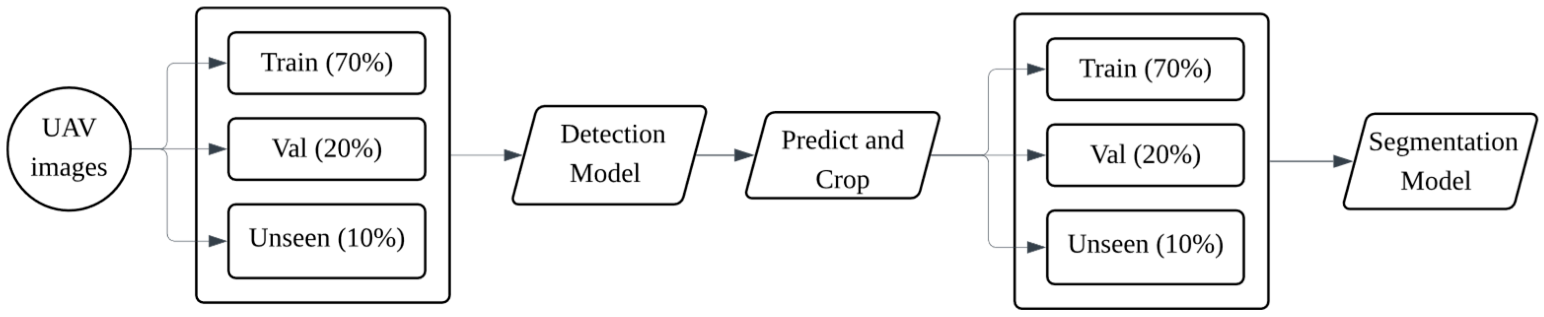
Figure 2.
Proposed framework.
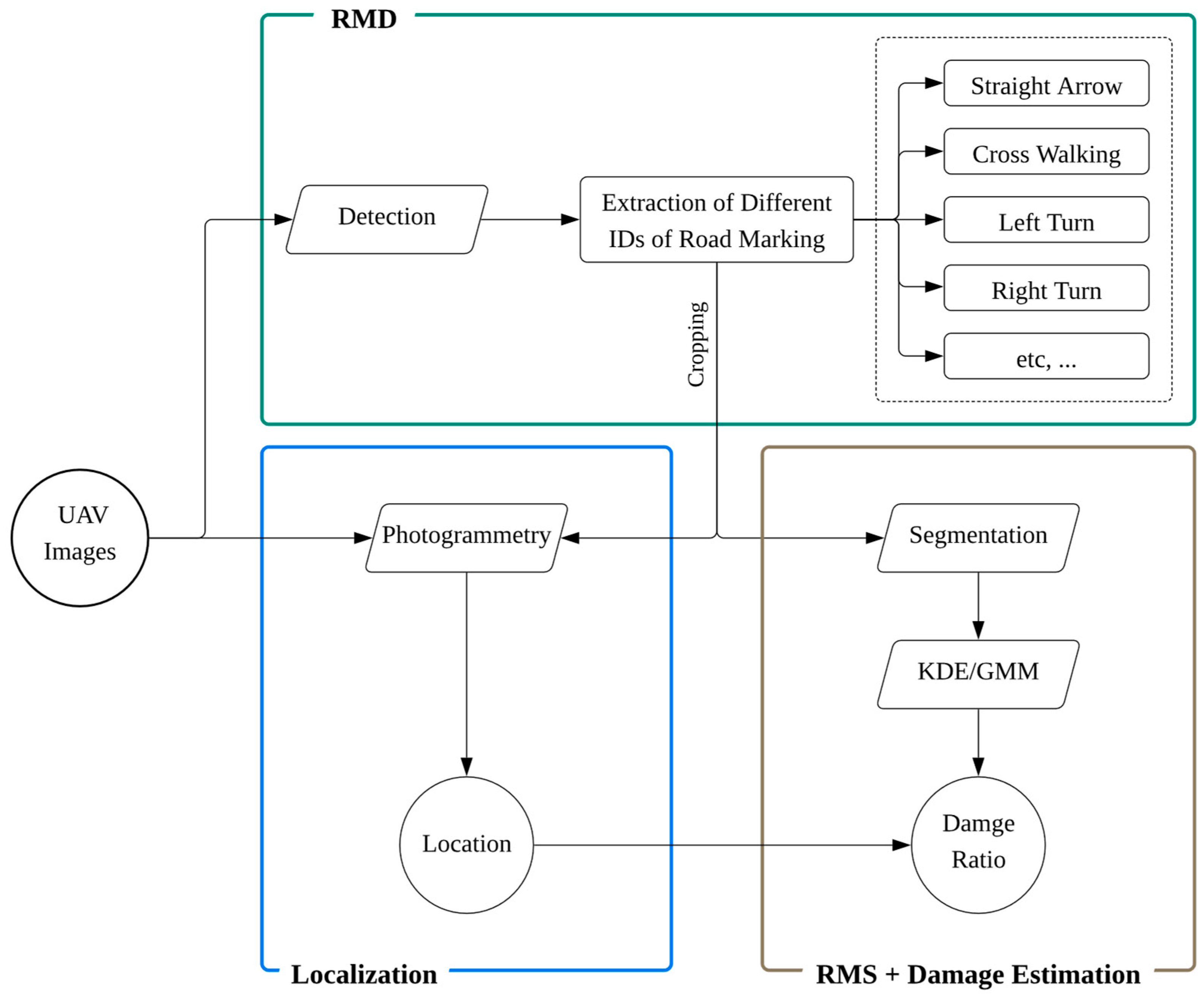
Figure 4.
VGG16-UNet architecture for segmentation.
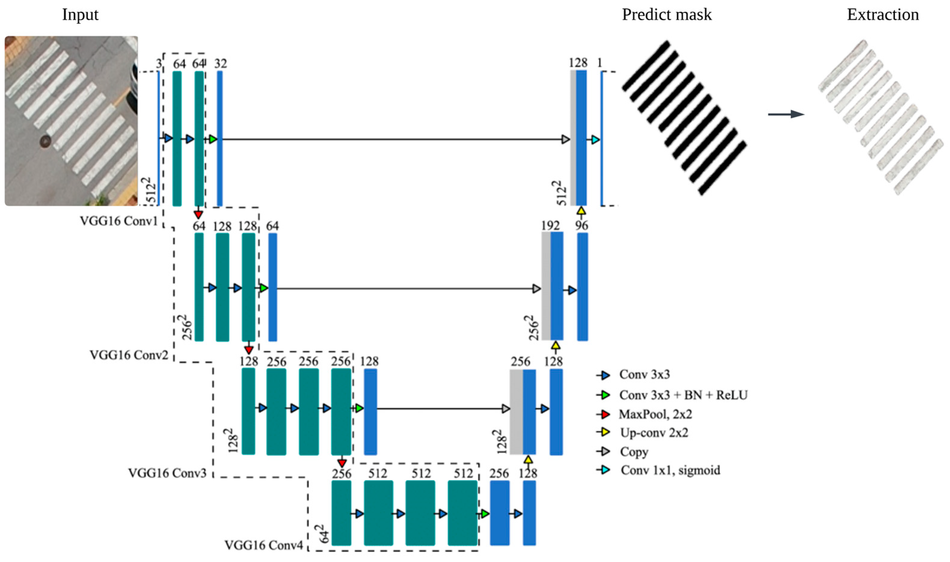
Figure 5.
Example of Yolov9e experiments.
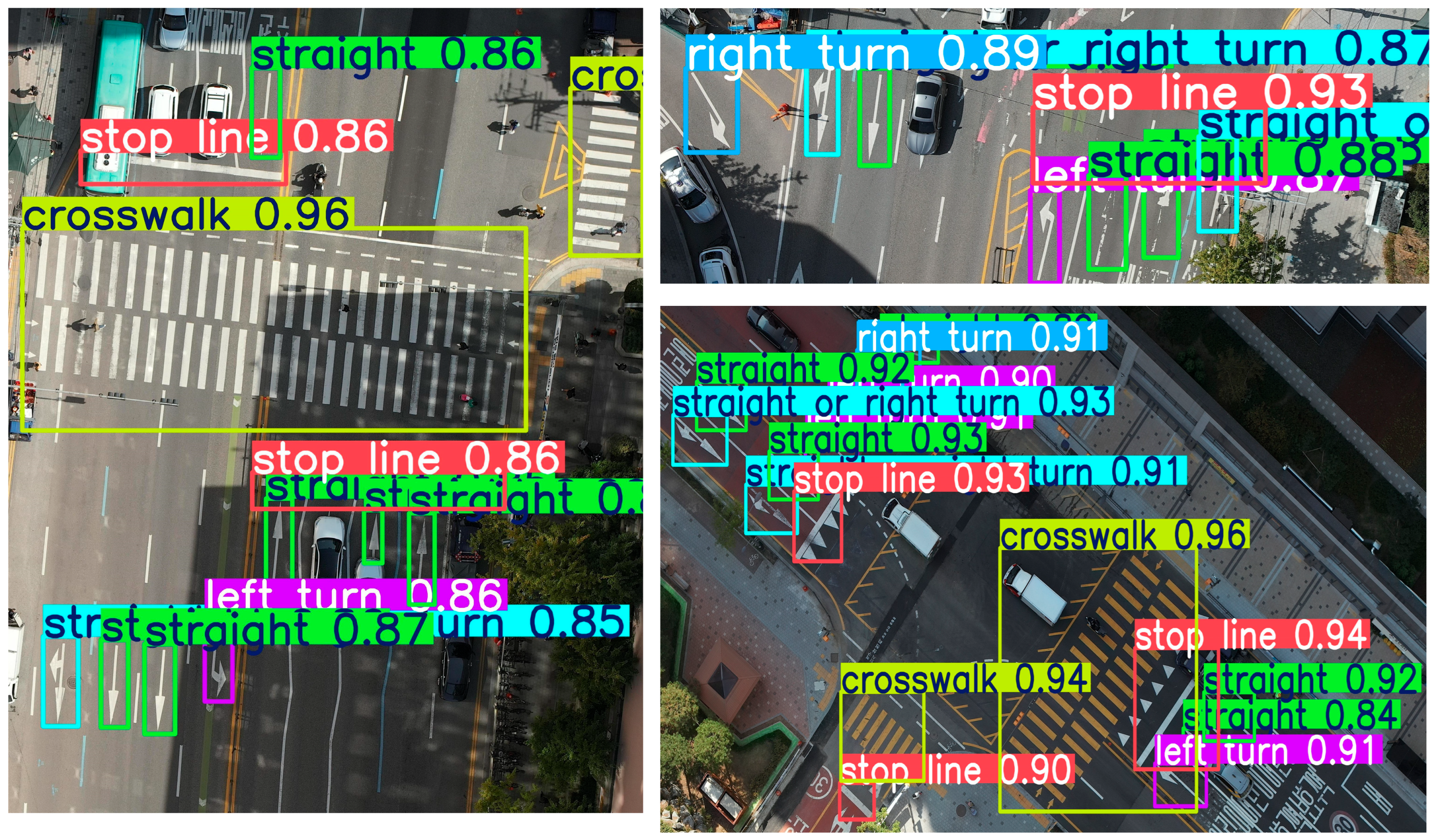
Figure 6.
Examples of VGG16-U-Net segmentation results. Top row: original crops (arrows, turn symbols, dense crosswalk bars). Bottom row: predicted masks.
Figure 6.
Examples of VGG16-U-Net segmentation results. Top row: original crops (arrows, turn symbols, dense crosswalk bars). Bottom row: predicted masks.
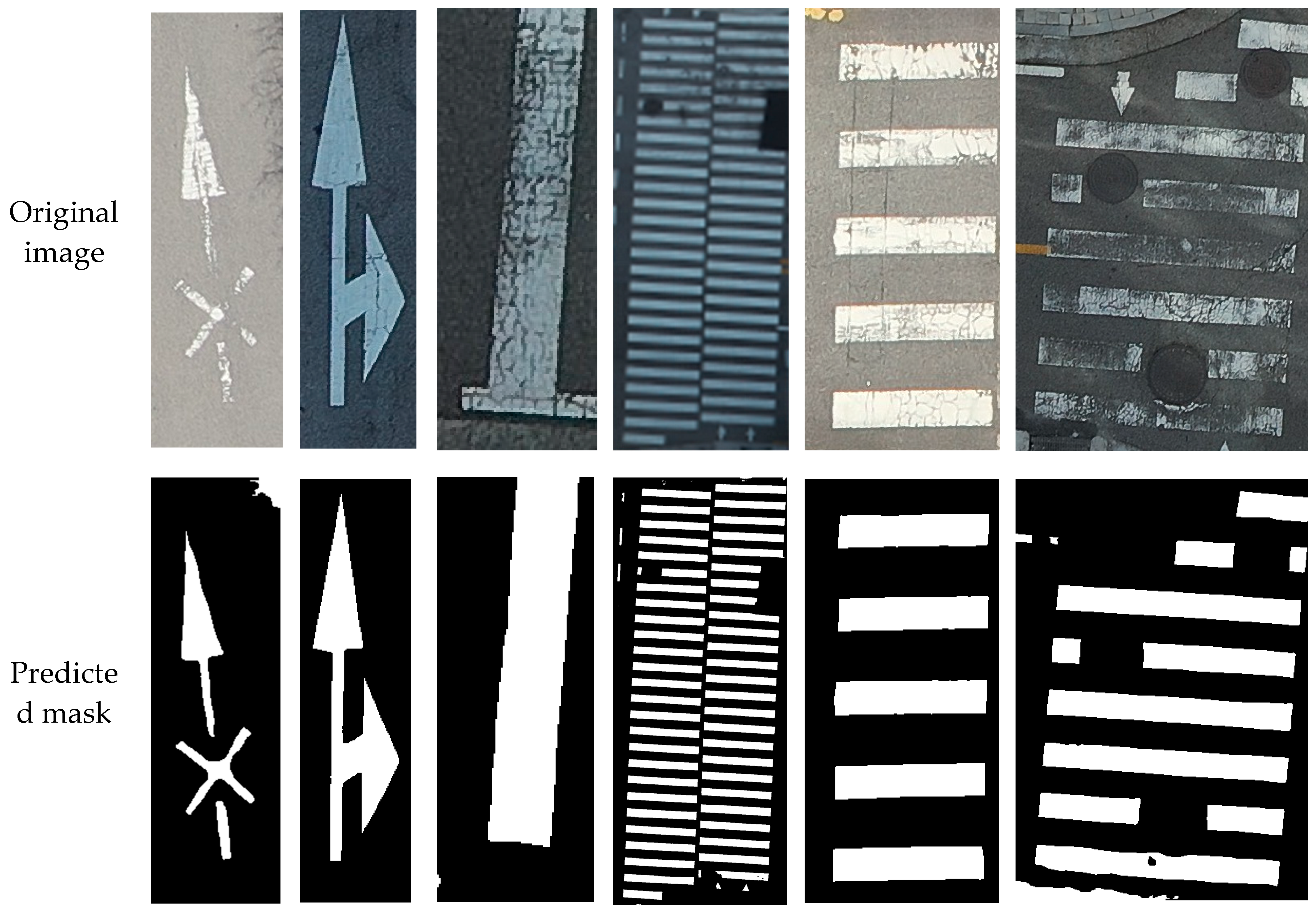
Figure 7.
Example of damage estimation on a road marking instance.
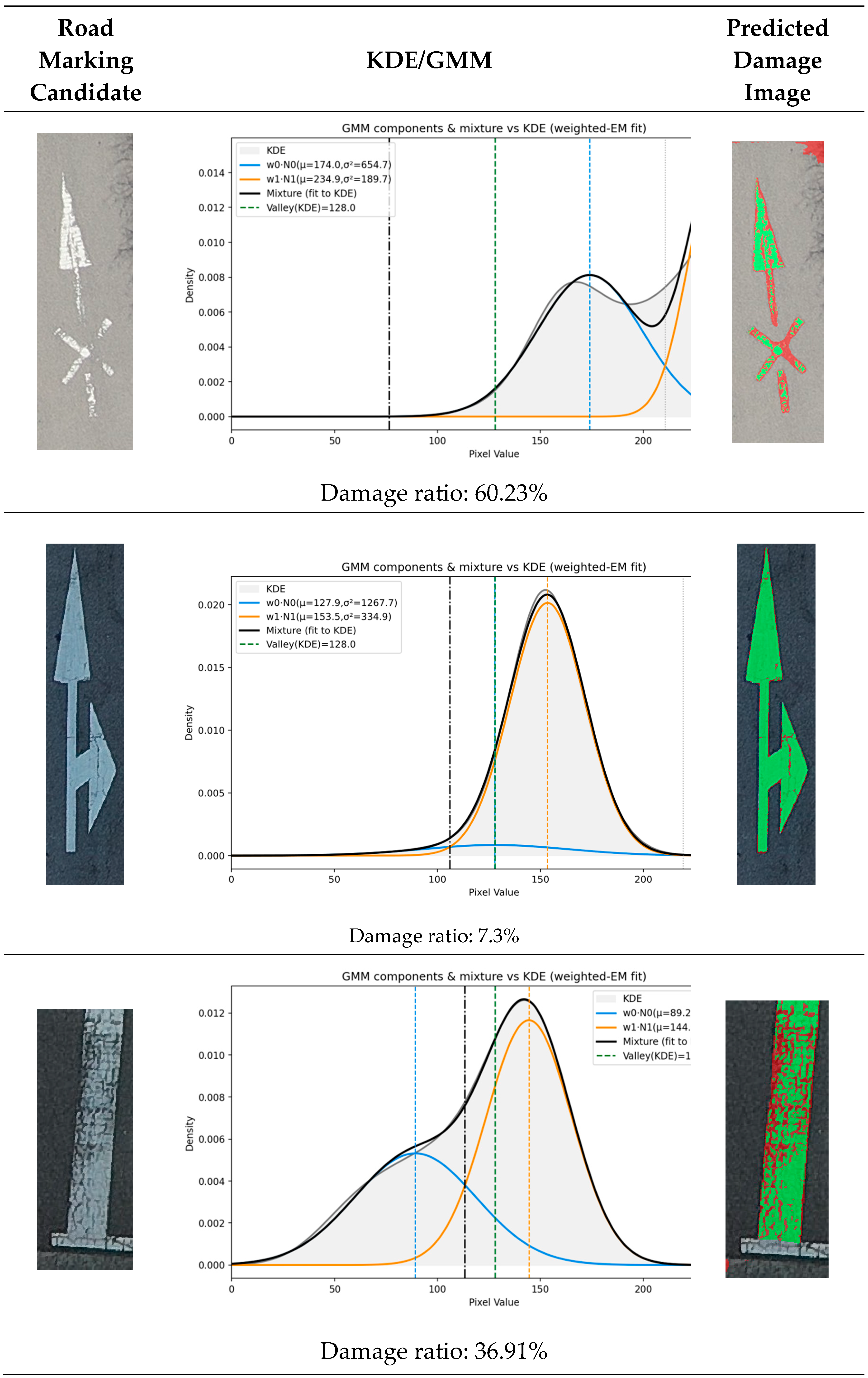
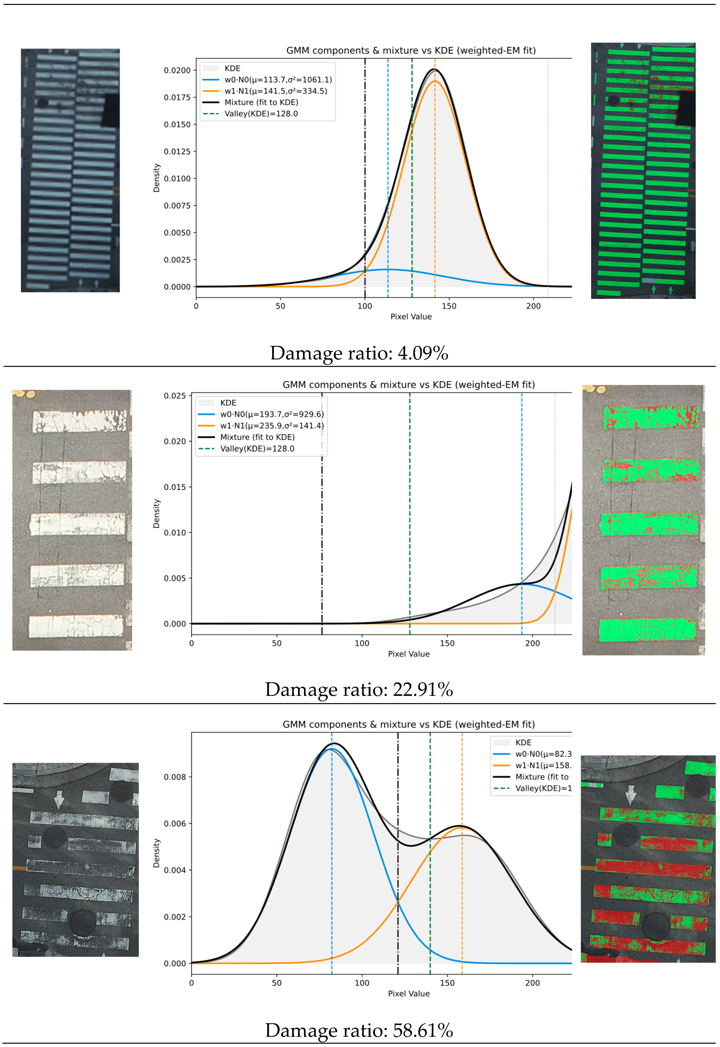
Figure 8.
Multi-method for damage extraction (a) GMM direct. (b) KDE/GMM. (c) K-means. (d) Otsu. (e) Damage ratio of each method.
Figure 8.
Multi-method for damage extraction (a) GMM direct. (b) KDE/GMM. (c) K-means. (d) Otsu. (e) Damage ratio of each method.
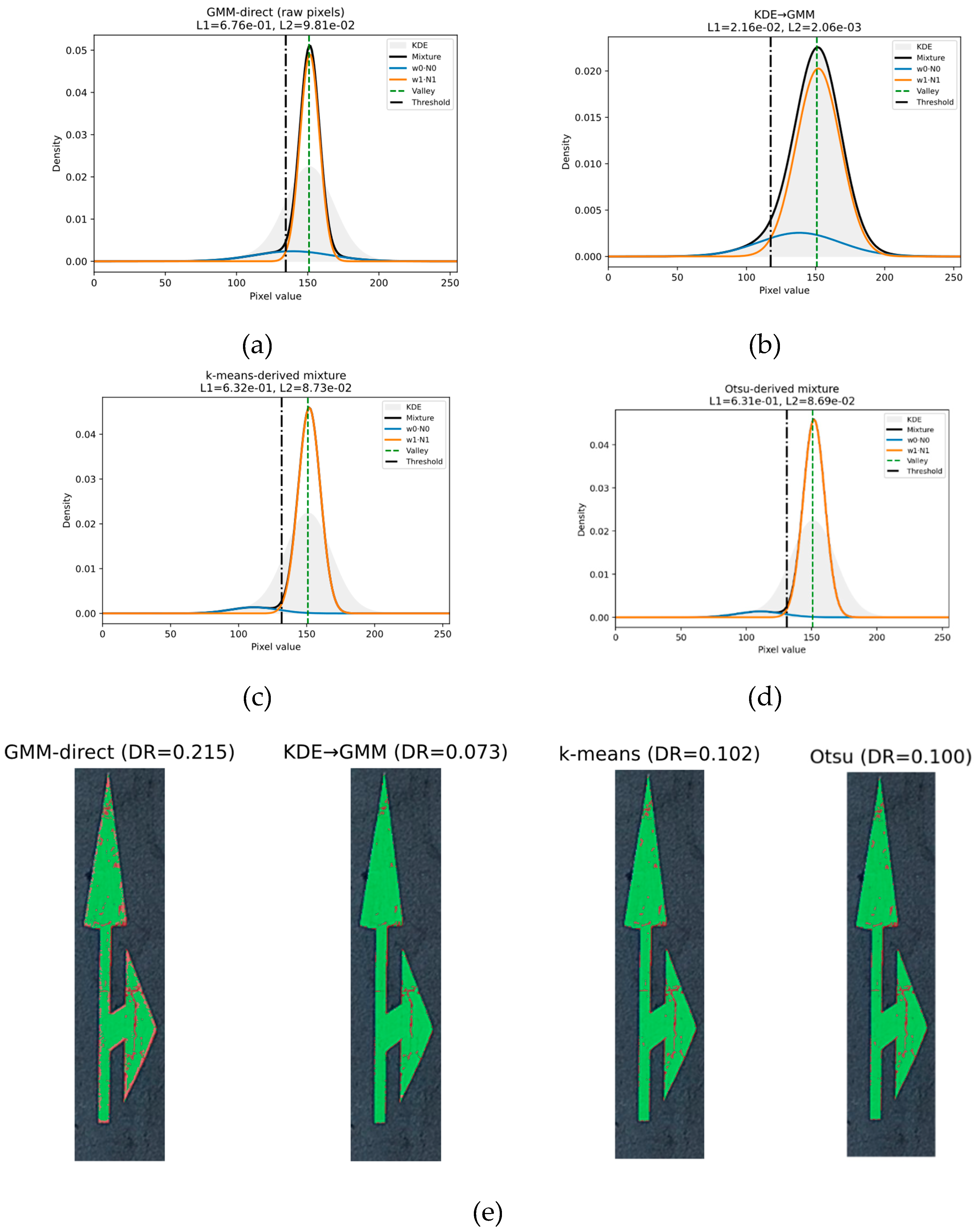
Figure 9.
Instance-wise comparison of predicted vs. ground truth damage.
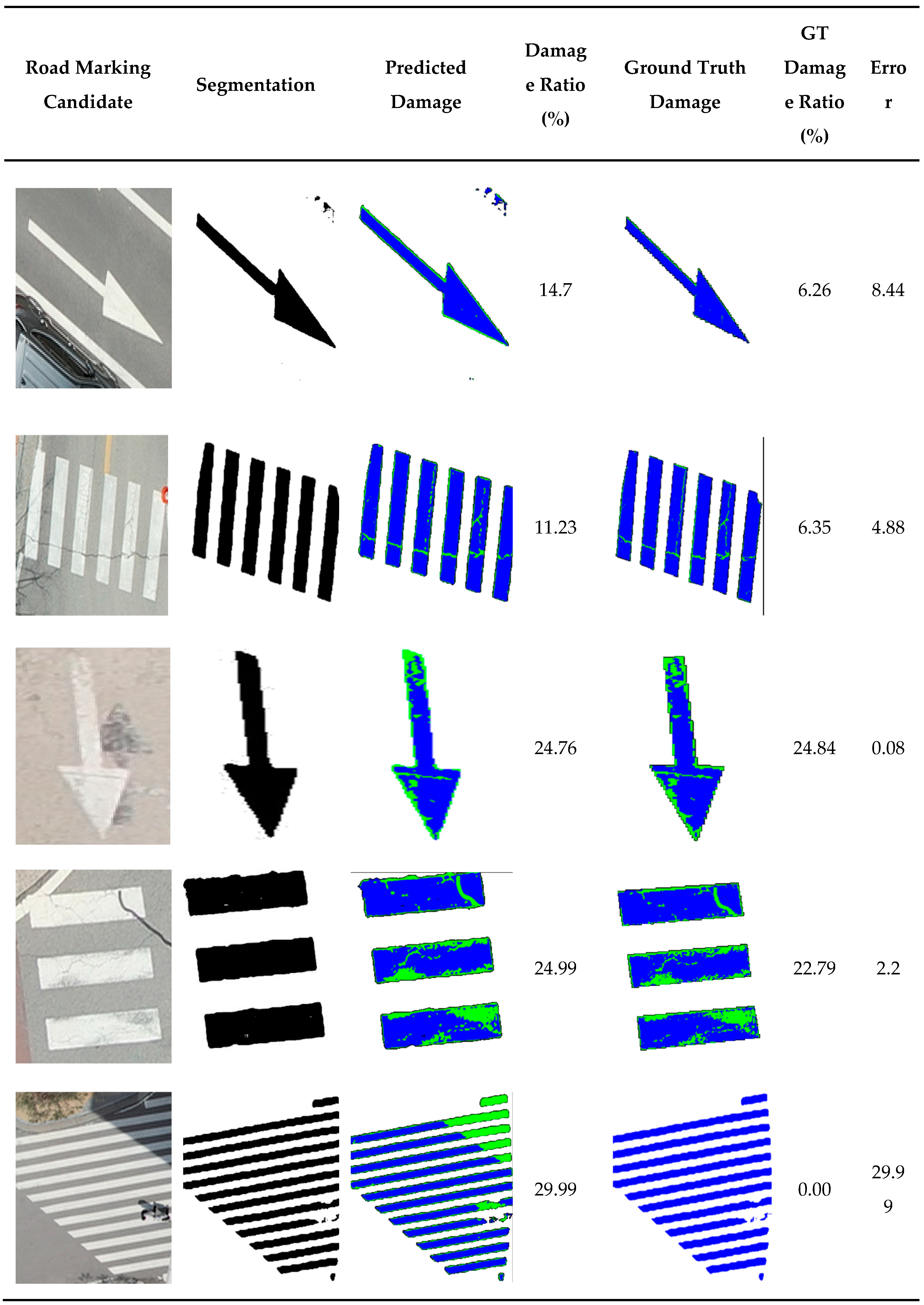
Figure 10.
Point cloud cleaning of the 3D reference model (top: before; bottom: after).
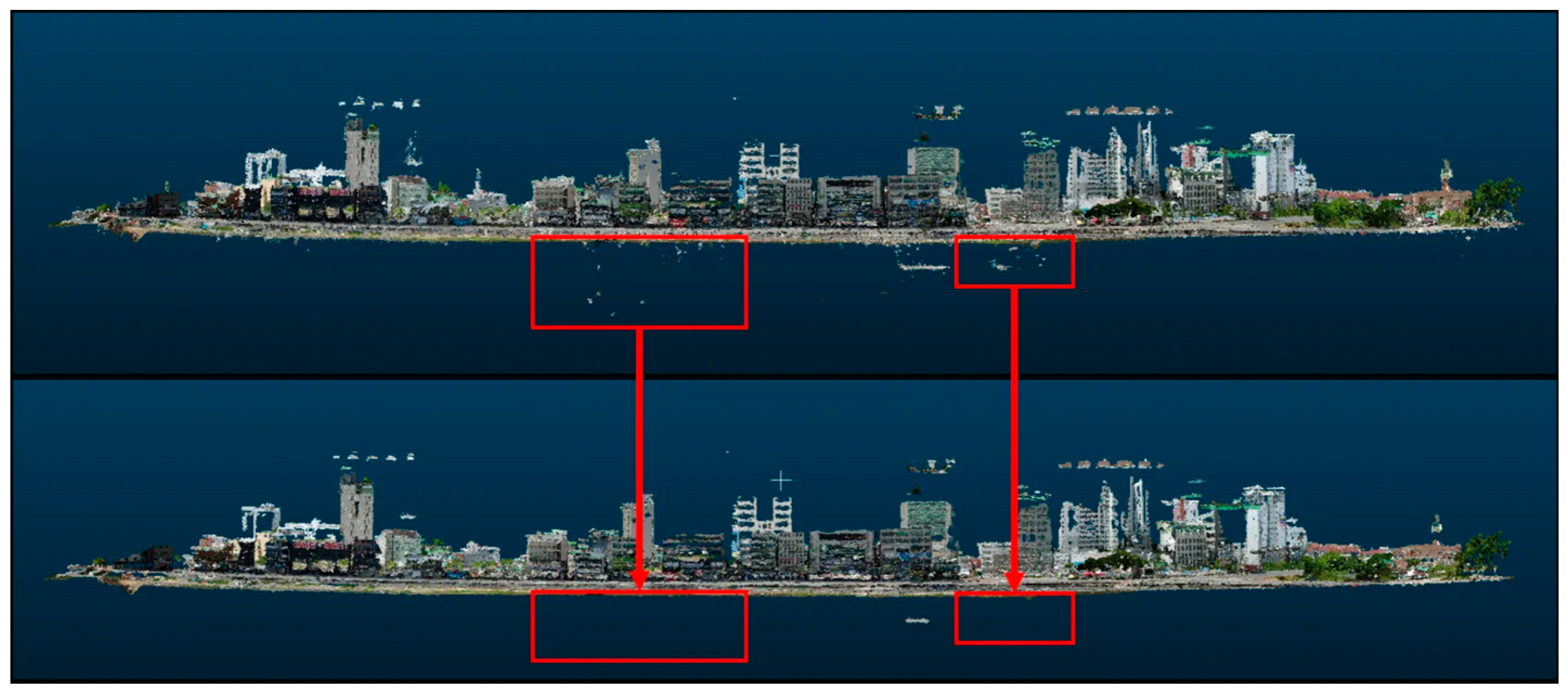
Figure 11.
3D position information associated with input image keypoints (blue dots) is based on the reference model.
Figure 11.
3D position information associated with input image keypoints (blue dots) is based on the reference model.
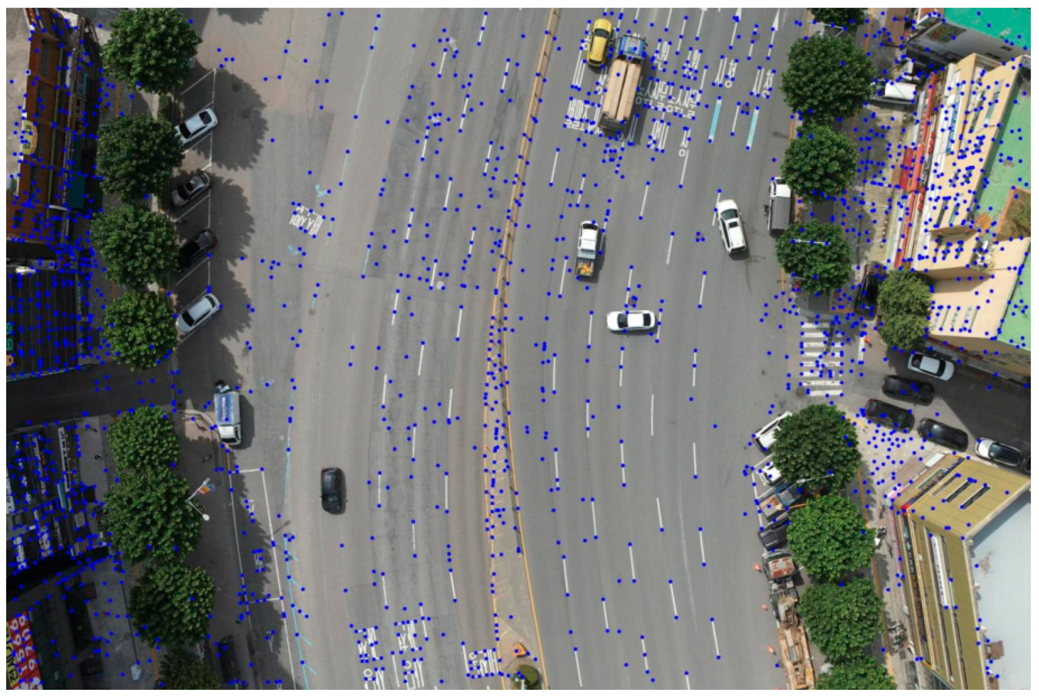
Figure 12.
(a) Detected objects in the input image; (b) estimated absolute 3D coordinates for each detected object.
Figure 12.
(a) Detected objects in the input image; (b) estimated absolute 3D coordinates for each detected object.
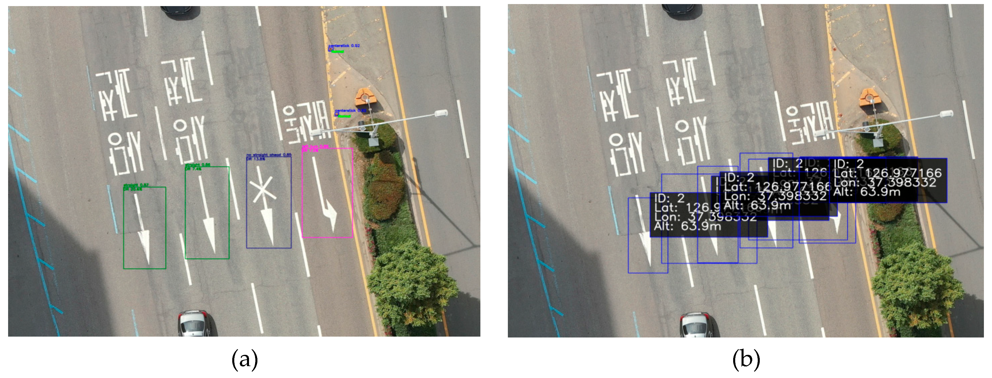
Figure 13.
Visualization of localization results on Google Earth (Suseo Station, Korea).
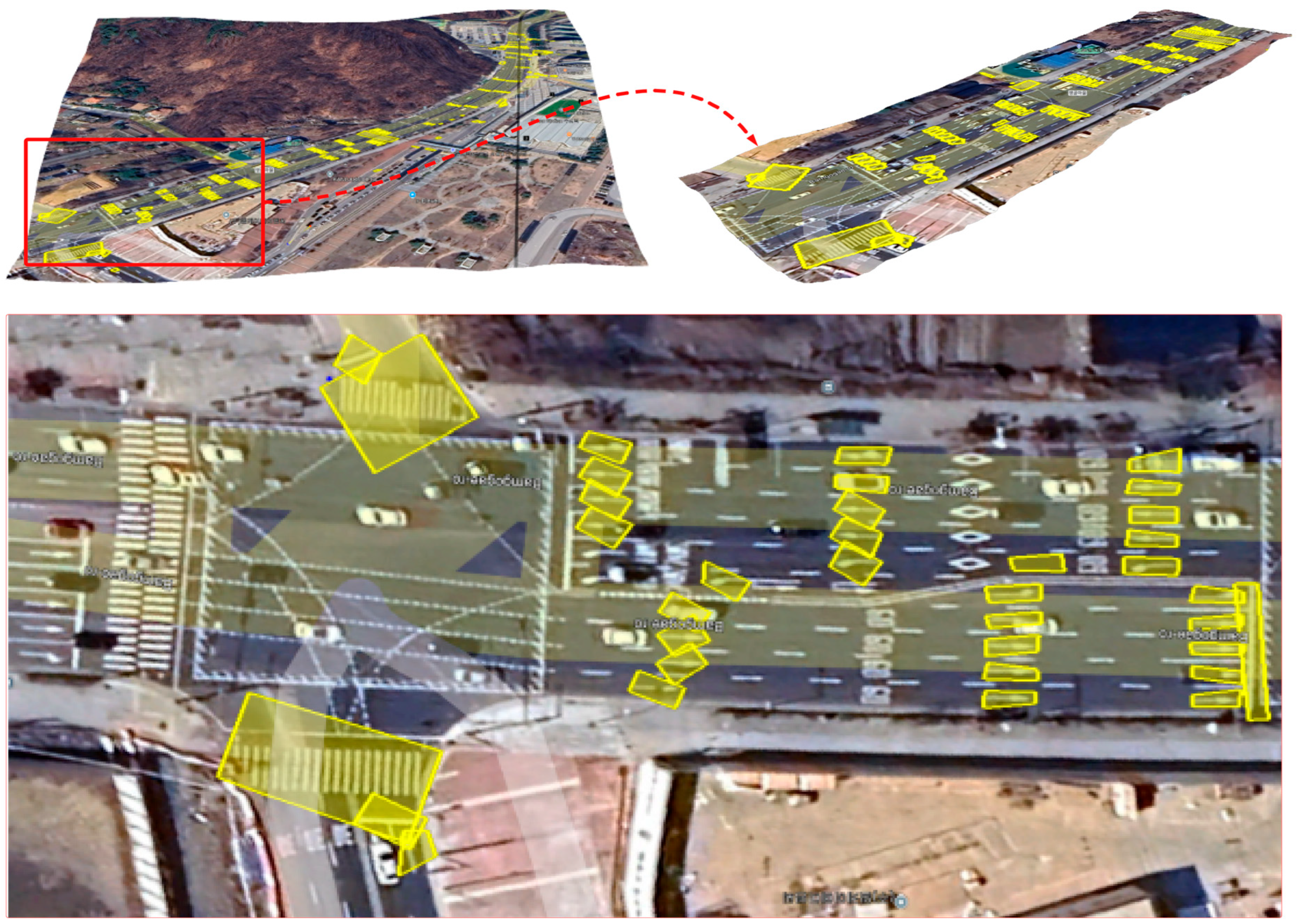

Table 1.
Flight planning parameters.
| Overlap | Sidelap | Flight Altitude | Ground Sampling Distance (GSD) |
|---|---|---|---|
| 80% | 70% | 100 meters | 0.6 centimeters |
Table 2.
Camera and sensor specification parameters.
| Sensor Size | Resolution | Focal Length | Image Format |
|---|---|---|---|
| 13.2 mm x 8.8 mm | 5,472 x 3,648 pixels | 9 milimeters | JPEG |
Table 3.
Training experiments of different YOLO versions.
| Model | Precision (%) | Recall (%) | F1 (%) | mAP50 (%) | mAP50-95 (%) | Speed (ms per image) |
GFLOPs |
|---|---|---|---|---|---|---|---|
| YOLOv8x | 95.506 | 90.592 | 92.984 | 94.764 | 64.256 | 0.6 | 257.5 |
| YOLOv9e | 95.363 | 91.982 | 93.642 | 95.497 | 65.553 | 0.8 | 189.2 |
| YOLOv10x | 95.451 | 90.669 | 92.999 | 95.803 | 64.757 | 0.1 | 160.0 |
| YOLOv11x | 95.556 | 91.66 | 93.567 | 95.693 | 64.478 | 0.5 | 172.6 |
| YOLOv12x | 95.402 | 91.583 | 93.454 | 95.433 | 64.749 | 1.3 | 198.6 |
Table 4.
Model training and evaluation using different methods of segmentation.
| Model | mIoU | F1 | MAE | ||||||
|---|---|---|---|---|---|---|---|---|---|
| Train | Val | Unseen | Train | Val | Unseen | Train | Val | Unseen | |
| Densenet201-UNet [27] | 95.09 | 95.30 | 93.88 | 97.46 | 97.57 | 96.81 | 1.73 | 1.65 | 2.33 |
| Unet [3] | 94.11 | 94.58 | 93.84 | 96.97 | 96.93 | 96.72 | 1.95 | 1.86 | 2.25 |
| VGG16 - UNet | 95.53 | 95.60 | 94.21 | 97.69 | 97.73 | 97.00 | 1.49 | 1.42 | 2.12 |
| GCN [28] | 93.5 8 | 93.72 | 92.58 | 96.72 | 96.71 | 95.95 | 2.12 | 2.10 | 2.82 |
| Upernet [29] | 94.87 | 95.18 | 93.79 | 97.36 | 97.28 | 96.59 | 1.71 | 1.62 | 2.28 |
| Deeplab HDC DUC [30] | 90.6 | 90.76 | 90.44 | 95.08 | 94.91 | 94.84 | 3.12 | 3.09 | 3.53 |
| PSPnet [31] | 69.77 | 71.76 | 72.86 | 80.89 | 82.44 | 83.47 | 3.32 | 3.35 | 4.34 |
Table 5.
Outcomes of methodological evaluation.
| Method | IAE median | ISE median |
|---|---|---|
| KDE/GMM | 0.021 | 0.002 |
| Otsu | 0.063 | 0.086 |
| k-means (k=2) | 0.063 | 0.087 |
| GMM-direct | 0.067 | 0.098 |
Table 6.
Illustration of final results at Suseo Station, Korea (samples shown).
| Identfication (ID) | Location | Condition (Pecentage of Damage %) |
|
|---|---|---|---|
| Latitude | Longtitude | ||
| Crosswalk | 37° 28' 55.9" N | 127° 06' 16.38" N | 3.5 |
| Left Turn | 37° 29' 15.89" N | 127° 06' 04.04" N | 20.0 |
| Right Turn | 37° 29' 13.67" N | 127° 06' 08.32" N | 7.1 |
| Right Turn | 37° 29' 13.12" N | 127° 06' 08.32" N | 53.8 |
| Straight and Left Turn | 37° 28' 56.78" N | 127° 06' 16.38" N | 25.4 |
| Straight Arrow | 37° 28' 56.80" N | 127° 06' 16.52" N | 58.5 |
| Straight Arrow | 37° 28' 56.82" N | 127° 06' 16.63" N | 2.7 |
Disclaimer/Publisher’s Note: The statements, opinions and data contained in all publications are solely those of the individual author(s) and contributor(s) and not of MDPI and/or the editor(s). MDPI and/or the editor(s) disclaim responsibility for any injury to people or property resulting from any ideas, methods, instructions or products referred to in the content. |
© 2025 by the authors. Licensee MDPI, Basel, Switzerland. This article is an open access article distributed under the terms and conditions of the Creative Commons Attribution (CC BY) license (http://creativecommons.org/licenses/by/4.0/).
Copyright: This open access article is published under a Creative Commons CC BY 4.0 license, which permit the free download, distribution, and reuse, provided that the author and preprint are cited in any reuse.


