1. Introduction
The marine environment holds abundant mineral and biological resources. In recent years, global demand for ocean exploration has grown rapidly. However, this progress is hindered by low-quality underwater images. The significant differences in physical properties between water and air cause severe degradation in underwater images, such as color casts, reduced contrast, blur, and noise1. Increasing depth exacerbates light scattering and absorption, while insufficient ambient light leads to extreme darkness. These issues limit the usability of underwater imagery. Thus, enhancing underwater images is crucial for marine exploration, and benefits tasks such as underwater detection2, vehicle navigation3, and marine biology research4.
Initial approaches to underwater image enhancement were based on physical models and statistical techniques. Optical models and attenuation estimation were used to restore images, with brightness and color correction reducing scattering effects. Some employed additive noise models or underwater transmission models for inverse restoration5. Histogram equalization adjusted luminance to enhance contrast while avoiding over-enhancement6. However, underwater complexity limits the accuracy of such models, and prior assumptions often fail under varying conditions. Consequently, these methods remain prone to noise, artifacts, and residual distortions, especially in challenging environments.
Lately, progress in UIE has been significantly propelled by deep learning. Data-driven models can learn feature representations automatically, improving image quality significantly. Common architectures include CNNs7, U-Net, and ResNet, while GANs8 show strong performance in generating visually realistic results. A significant innovation is the Vision Transformer (ViT)9, which substitutes convolution with self-attention and excels at modeling long-range dependencies. This enables ViT to handle global context and fine details, addressing issues like color distortion and contrast loss. However, ViTs lack CNNs’ local inductive bias, limiting their ability to capture fine local features, and their high computational cost increases inference time.
Therefore, this paper introduces UCA-Net, a lightweight underwater image enhancement network based on a hybrid CNN-Transformer architecture. By jointly optimizing global color correction and local detail enhancement, UCA-Net achieves excellent visual quality with low parameter complexity. Specifically, we first design the Depthwise Separable Convolutional Residual Attention Composite Block (DCRAC), which integrates multiple attention types and residual connections to enhance textures and reduce blurring and noise in degraded regions. Next, we propose the Deformable Convolution-Transformer Block (DCTB), where the deformable convolution layer adapts to underwater geometric distortions. The Frequency-Domain Feature Fusion Module (FDFM) ensures the organic fusion of the two output features to achieve more optimal utilization of features. Meanwhile, a dual-path channel attention transformer learns global color distribution and illumination conditions, improving color shifts and low contrast. These modules are embedded in a U-shaped encoder-decoder framework: The encoder gradually extracts multi-scale features through DCRAC, DCTB fuses global context at the bottleneck layer, The decoder uses skip connections to reconstruct detailed enhanced images, completing the UIE task. The main contributions are summarized below:
We designed UCA-Net, an innovative underwater image enhancement U-shaped network based on the combination of CNN and Transformer. This network has a good enhancement effect, is very effective for the restoration of global and local colors and details, and has a lightweight architecture and a relatively low number of parameters.
We proposed the Transformer module DCTB (Deformable Convolution-Transformer Block), which consists of a prestructure composed of deformable convolution and a dual-path channel attention Transformer module containing adaptive learning parameters. At the same time, it takes into account the effect of enhancing local details and paying attention to overall information.
We design a feature fusion module in the frequency domain, which establishes a balance mechanism between frequency selective enhancement and information retention, which is particularly beneficial for scenarios such as underwater image enhancement.
We conducted a large number of comparative experiments on multiple datasets to prove that UCA-Net is superior to the existing advanced methods while maintaining a smaller number of parameters and model complexity.
2. Related Works
Recently, techniques for underwater image restoration and enhancement are primarily classified into two categories: traditional and deep learning-based approaches. Traditional methods can further be categorized into statistical-based and physical model-based approaches.
Statistical methods enhance underwater images using heuristic pixel operations rather than modeling light propagation. For instance, Hitam et al.10 employed contrast-limited adaptive histogram equalization to improve contrast and suppress overexposure. Zhang et al.11 applied segmented color correction and dual-prior optimization to enhance detail and restore natural colors. Ancuti et al.12 fused multiple exposures to optimize color and visibility. Zhang et al.13 combined multi-scale Retinex with a physical underwater model for comprehensive restoration.
Physical model-based methods enhance underwater images by reversing light propagation, requiring accurate environmental parameters and priors like the dark channel14 and red channel15. Li et al.16 proposed a defogging framework combining a physical model with histogram priors to preserve detail and restore color. Peng et al.17 used a joint model to estimate transmittance, correct color, and iteratively restore radiance considering blur and absorption. Galdran et al.18 introduced adaptive red channel recovery based on light attenuation. However, these methods are sensitive to environmental changes and heavily rely on accurate priors, limiting their robustness in complex conditions.
Deep learning has greatly advanced underwater image enhancement (UIE), mainly through CNNs and GANs. CNN-based methods are predominant. Li et al.19 proposed UWCNN, a lightweight CNN using underwater scene priors, and trained on synthetic data representing 10 water types to model wavelength-specific absorption for color and visibility correction. Naik et al.20 introduced Shallow-UWNet, a compact network for effective enhancement. Yan et al.21 designed a dynamic, attention-guided multi-branch model to improve image quality. Qi et al. 22 proposed UICoE-Net, a collaborative framework using feature matching and joint learning to enhance contrast and color consistency.
Generative Adversarial Networks (GANs) are neural networks that optimize image generation through an adversarial process between a generator and discriminator, and have been widely applied in image generation and style transfer. Yang et al.23 proposed a Conditional GAN (CGAN) using U-Net as the generator and PatchGAN as the discriminator. By inputting degraded underwater images, their model progressively produces clearer, more realistic outputs through adversarial training. Islam et al.24 introduced a fast underwater image enhancement method incorporating depth-separable convolution and channel attention, significantly reducing parameters and computational complexity. Li et al.25 developed an unsupervised generative network, WaterGAN, which combines underwater optical scattering models and color transmission characteristics to generate high-quality enhanced images. Chen et al.26 presented PUIE-Net, a perception-driven enhancement network that balances visual quality and physical authenticity by embedding deep learning with physical priors.
Architectures based on Transformers have recently demonstrated robust performance in computer vision tasks, owing to their capacity for global modeling. Swin Transformer27 reduces computation via local windows and shifted windowing, improving cross-region interaction. UIEFormer by Qu et al.28 uses a lightweight hierarchical Transformer with cross-stage fusion and adaptive color correction, enhancing contrast and fidelity. URSCT, proposed by Ren et al.29, combines dual convolutions with attention for better detail restoration. BCTA-Net by Liang et al.30 introduces a two-level color correction scheme, merging global color stats with local pixel refinement to avoid over-correction and detail loss.
3. Proposed Method
In this section, we will introduce the relevant details and structure of UCA-Net in detail. As shown in the figure, UCA-Net adopts the classic UNet network architecture as the main structure, and the overall manifestation is an encoder-decoder network with skip connections. The initial input was an underwater distorted image 𝐿𝑎𝑙𝑙 = 𝛼1𝐿𝑙1 + 𝛼2𝐿𝑆𝑆𝐼𝑀 + 𝛼3𝐿𝑝𝑒𝑟𝑐, after the image passes through a convolutional layer, the network will generate low-level features 𝐹0 ∈ 𝑅𝐻×𝑊×𝐶 (C represents the number of channels), it is then fed into the subsequent encoder-decoder network for deeper-level processing and feature fusion. The initial information is first fed into the joint module Parallel Transformer-CNN Hybrid Module(PTCHM). In the subsequent ADSB module, the input features are re-weighted along the channel dimension using a multi-head self-attention mechanism to further capture global contextual representations 𝐹𝐺 ∈ 𝑅𝐻×𝑊×𝐶. Meanwhile, DCRAC extracts and processes the local feature 𝐹𝐿 ∈ 𝑅𝐻×𝑊×𝐶 through the connection of multiple convolutional layers and identities as well as the construction of a composite attention module. During this process, each encoder will connect its output to the corresponding peer decoder, achieving the fusion of some features between the encoder and the decoder. The overall network is divided into five layers, each of which is composed of a combined module of DCRAC and ADSB, as well as FDFM. Finally, after passing through another convolutional layer, we will obtain the output restored image I0 . Next, we will explain the design and mechanism of each module, illustrate its corresponding functions and contributions in the entire enhancement task.
Figure 2.
Architecture of UCA-Net. From (a) to (d) is overall structure, PTCHM, DSCRC and DCTB.
Figure 2.
Architecture of UCA-Net. From (a) to (d) is overall structure, PTCHM, DSCRC and DCTB.
3.1. PTCHM
A central element of UCA-Net is the Parallel Transformer-CNN Hybrid Module (PTCHM). As depicted in Figure 1, this module contains a primary unit known as the Transformer-CNN Unit (TCU), which integrates CNN and Transformer branches in a parallel configuration. The PTCHM leverages the strengths of both CNNs and Transformers: the Transformer branch allocates weights to global features and captures long-range dependencies, while the CNN branch is effective in extracting local features and fine details. Combining these allows PTCHM to adjust global image properties (e.g., color, contrast, brightness) while preserving local textures and details, resulting in superior performance for underwater image enhancement tasks. The TCU is composed of three primary sub-networks: 1) the Depthwise Separable Convolutional Residual Attention Composite Block (DCRAC), which employs depthwise separable convolutions, residual connections, and a Composite Attention Module (CAM) to minimize computational load while maintaining feature richness; 2) the Deformable Convolution-Transformer Block (DCTB), featuring deformable convolution layers and an Adaptive Dual-path Self-Attention Block (ADSB); and 3) the FDFM, which decomposes spatial features into frequency components via the discrete cosine transform (DCT) to enable more sophisticated feature integration compared to conventional element-wise operations. This hybrid design allows the model to adapt to geometric variations while capturing long-range dependencies, enhancing its ability to process complex underwater scenes.
3.2. DCRAC
The effective application of underwater images frequently necessitates the enhancement of fine details and texture features. However, due to various degradation factors, underwater images often suffer from detail loss and blurring. To improve the network’s capability for reconstructing and restoring local fine-grained features, we designed the DCRAC module. Specifically, DCRAC is composed of three residual convolutional modules constructed using depthwise separable convolutions, combined with a Compound Attention Module (CAM). In each depthwise separable convolution, we apply a channel reordering technique to address the information barrier issue caused by independent channel computations in depthwise separable convolutions. This enhancement improves the feature representation capability of the convolutional layers. The Compound Attention Module (CAM) we designed is composed of parallel spatial and channel attention branches, followed by a pixel-level attention mechanism. The entire CAM operates in a coarse-to-fine manner: first, the input features are processed through the channel and spatial attention modules, where the respective channel attention weights and spatial attention weights are computed sequentially. These weights are then used to recalibrate the features, allowing the network to adaptively emphasize the importance of different regions within the feature map. The two parallel attention modules independently process the input features, assigning unequal weights to different channels and pixels, thereby enhancing the overall feature representation for image enhancement. Following this, a pixel attention module is employed to fully integrate the outputs from the previous two attention branches. This enables pixel-wise weight allocation, which further refines the regional representations. Through this multi-level refinement process, the network progressively enhances and strengthens feature representations across different levels of abstraction, ultimately achieving more precise and discriminative feature expression. As shown in
Figure 2, the CAM module further fine-tunes the processing of fine-grained details, thereby enhancing the block’s overall performance in local feature enhancement. When the input is given as 𝑋 ∈ 𝑅
𝐻×𝑊×𝐶, the feature map is first passed through both the spatial attention and channel attention branches, which generate their respective outputs. This dual-branch mechanism enables the module to decouple spatial contextual dependencies from channel-wise semantics, allowing for a more structured refinement of feature activations. By attending to where and what to focus on, the module achieves a synergistic enhancement of salient patterns in underwater imagery.
The output SA(X) and CA(X), after feature stitching, will be input into the pixel attention module:
After the input feature map 𝑋 ∈ 𝑅
𝐻×𝑊×𝐶 passes through the first 3×3 depthwise separable convolutional layer, it is followed by a Dropout layer, which randomly deactivates a portion of the feature units to suppress overfitting during training. Subsequently, a ReLU activation function is applied to introduce non-linearity into the network, enabling it to better model complex patterns within the data. The attention-weighted feature map obtained from the CAM is subsequently passed into a depthwise separable convolutional layer, where it undergoes further transformation. This is followed by a Dropout operation, The output is then passed through a ReLU activation function, introducing non-linearity and enabling the network to learn more expressive features. To facilitate more efficient training, the output feature is then fused with the original input via a residual connection, which helps preserve low-level information and accelerates model convergence. The integration of Dropout and residual learning establishes a balanced mechanism between regularization and information preservation, which is particularly beneficial in scenarios like underwater image enhancement where features may be sparse or degraded. The final output is:
3.3. DCTB
Deformable convolution
In UIE tasks, previous methods typically used standard or depthwise separable convolutions to extract local features from images or sequences. These approaches generally perform well in normal conditions by capturing basic structures and patterns. However, they have limitations in more complex environments. Underwater images and biological structures often feature irregularities, blurriness, and distorted object boundaries, such as drift or fragmentation. In these cases, traditional convolutions, which rely on fixed receptive fields and static sampling patterns, struggle to capture non-rigid targets or locally distorted features. This results in reduced receptive fields, distorted context, and weaker semantic coherence.
To address these issues, we introduce Deformable Convolution into the UIE framework to improve the network’s ability to model complex spatial structures. Unlike standard convolutions, deformable convolution uses learnable offset parameters, allowing the sampling locations to adapt based on the feature distribution. This flexibility overcomes the limitations of fixed grid sampling, improving the model’s ability to handle irregular boundaries, non-rigid shapes, and complex lighting conditions found in underwater environments. Deformable Convolution, first proposed by Kaiming He et al.31 in “Deformable Convolutional Networks”, was designed to overcome the limitations of conventional CNNs in handling geometric transformations and spatial deformations in visual data. We are the first to integrate deformable convolution into the UIE task, aiming to leverage its adaptive spatial sampling capability to handle the irregular and non-rigid structures typical of underwater imagery.
The core idea of deformable convolution is to add learnable offsets to the sampling positions of standard convolution, enabling the sampling points to dynamically adjust their positions according to the input content, thereby achieving an adaptive receptive field, as shown in
Figure 3. Specifically, for a traditional convolution operation, its output at position
can be expressed as:
Among them, R is the set of sampling points (such as the 9 positions of a 3×3 convolution), and w is the convolution weight. In deformable convolution, the sampling position becomes:
The offset term
for each sampling location in deformable convolution is learned from the input feature map using an additional convolutional layer. As illustrated in
Figure 3, this mechanism allows the shape of the convolutional kernel to adapt dynamically—from a fixed rectangular grid to a flexible, data-driven configuration. This adaptability significantly enhances the model’s ability to handle the complex, cluttered, and occluded nature of underwater environments. Crucially, this deformation of the sampling grid introduces no extra kernel parameters. Instead, it enables the convolution to expand its effective receptive field without increasing computational complexity or model size. This makes the operation both computationally efficient and capable of capturing non-rigid patterns and spatial variations, which are prevalent in underwater scenes.
We design the C (DCTB) by combining deformable convolution and self-attention to capture both spatial adaptability and contextual dependencies. The module begins with a residual block based on deformable convolution. Unlike traditional convolutions, deformable convolution uses learnable offsets to dynamically shift sampling locations, allowing the receptive field to adapt to complex image geometries. This adaptability is particularly effective for capturing key features in irregular or deformable objects—common in underwater organisms and terrains with complex textures and edges. To address such challenges, deformable convolution enhances the model’s ability to extract robust features across diverse scales, orientations, and shapes. By enabling the kernel to change shape and position based on input features, it significantly improves flexibility in capturing salient cues from non-rigid regions. This capability is further strengthened by the Adaptive Dual-path Self-Attention Block (ADSB), which models long-range dependencies and emphasizes globally relevant features. Together, deformable convolution and self-attention allow the network to more effectively recognize and represent complex structures in scenes with occlusion, irregularity, or poor visibility.
Underwater images often suffer from global color distortion, inconsistent tones, low contrast, and uneven illumination, all of which impair effective feature representation. To address these issues, we propose the Adaptive Dual-path Self-Attention Block (ADSB), designed to regulate global color and lighting, thereby enhancing the refinement of global features. Unlike standard Transformer-based attention mechanisms, which compute dense interactions across all tokens and channels—often introducing redundant computation and noise—the ADSB adopts a more efficient strategy. Specifically, it uses a dual-branch sparse-dense attention mechanism with adaptive scaling, selectively allocating computational resources based on the importance and spatial distribution of features. This design reduces computational load while preserving essential semantic and structural information, allowing the model to focus on visually relevant areas in underwater scenes. The ADSB includes a sparse attention branch guided by a sparsity operator , which filters out low- or negatively correlated query-key-value features. This helps the model focus on high-response regions, enhancing texture and edge information. To ensure that important global cues are not missed, a dense attention branch, guided by a complementary operator , is introduced to capture long-range dependencies and maintain contextual continuity. This branch helps correct global illumination imbalance and color bias. To integrate both branches, we employ an adaptive fusion strategy using learnable weights, allowing the model to dynamically balance the contributions from sparse and dense attention depending on the content and enhancement demands. This mechanism ensures task-specific optimization for complex underwater image enhancement.
In the ADSB module, the input feature tensor
is first processed via layer normalization to obtain the normalized representation
. This normalized tensor then passes through a 1×1 point-wise convolution followed by a 3×3 depth-wise convolution and flattening operation, producing the query (
), key (
), and value (
) representations, where:
Then our dense attention branch will obtain the global attention score through
:
Similarly, the sparse attention branch will also obtain the corresponding sparse attention score after and normalization operations:
Directly applying attention outputs from the two branches may lead to information loss and imbalanced weighting, which can impair the overall enhancement effect. To mitigate this, we introduce adaptive learnable parameters
,
to fuse the outputs of the sparse and dense branches. These parameters are normalized weights, enabling the model to dynamically balance the contributions of each branch based on feature relevance. This design ensures more stable and effective integration, maintaining the complementarity between localized saliency and global context.
This design enables the model to more effectively suppress irrelevant regions and assign greater attention to high-frequency feature areas, thereby improving the focus on salient structures. By introducing adaptive attention fusion, the model can dynamically adjust its reliance on sparse and dense attention branches during training. Such flexibility allows the network to automatically learn optimal attention patterns tailored to different tasks and datasets, ultimately achieving better generalization and performance across diverse conditions. This task-adaptive balance not only mitigates overfitting to redundant regions but also ensures robust feature enhancement in complex scenarios such as underwater imaging or low-visibility environments.
Figure 4.
Schematic diagram of the C (ADSB).
Figure 4.
Schematic diagram of the C (ADSB).
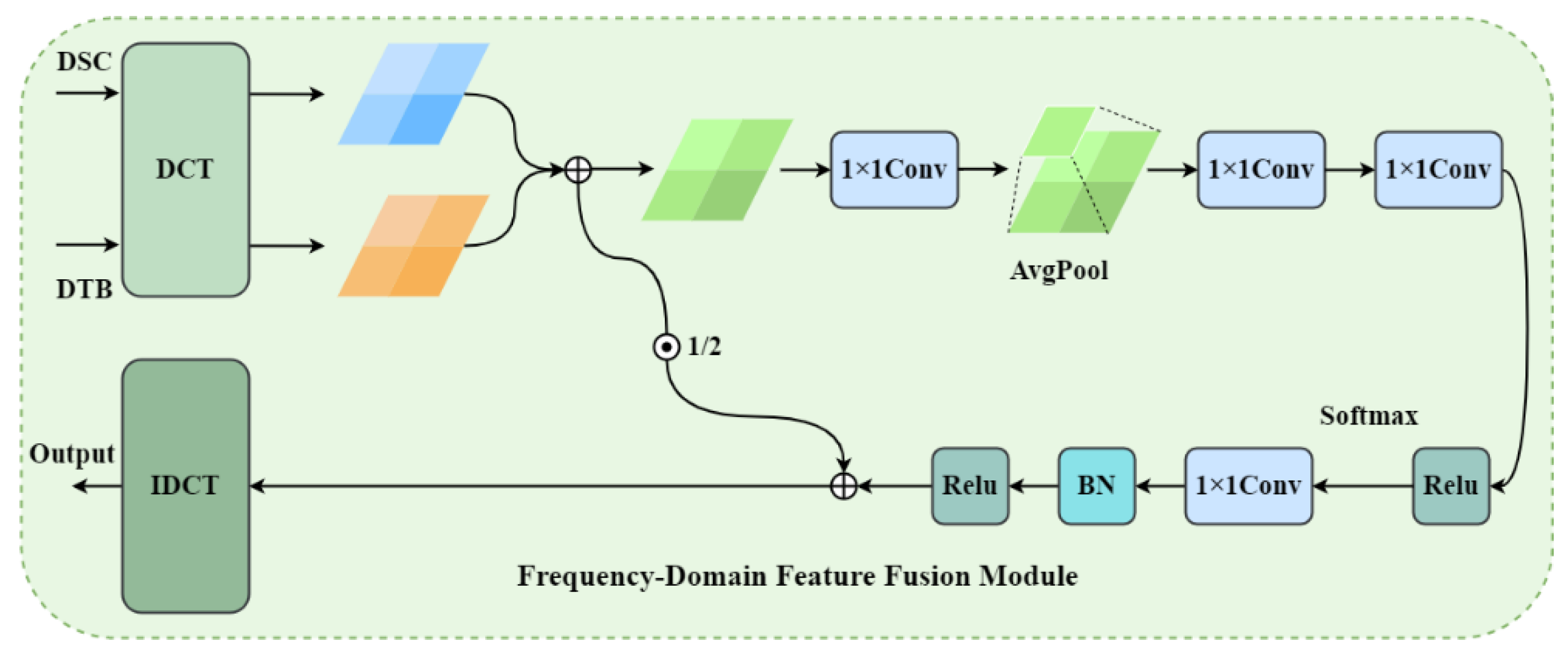
3.4. FDFM
To address the challenge of effectively integrating complementary features from different convolutional modules in underwater image enhancement networks, we propose a novel Frequency-Domain Feature Fusion Module (FDFM). This module leverages discrete cosine transform (DCT) to decompose spatial features into frequency components, enabling more sophisticated feature integration compared to conventional element-wise addition or concatenation approaches.
DCT
The Discrete Cosine Transform (DCT) serves as the mathematical foundation of our frequency-domain fusion approach. DCT is an orthogonal linear transformation that converts spatial-domain signals into frequency-domain representations, where the basis functions are cosine waves of varying frequencies. Mathematically, for a 2D signal f(x,y) of size M×N, the 2D DCT is defined as:
The key advantage of DCT over other frequency transforms lies in its energy compaction property: for natural images, most of the signal energy is concentrated in the low-frequency coefficients located in the upper-left corner of the transformed matrix, while high-frequency components (typically representing noise and fine textures) are distributed in the lower-right region. This property makes DCT particularly suitable for image enhancement tasks, as it naturally separates structural information from noise and artifacts.
In the context of our FDFM module, DCT plays a crucial role in enabling frequency-selective feature fusion. By transforming both DCTB and DCRAC features into the frequency domain, we can decompose each feature map into four distinct frequency bands—low-frequency (LL), mid-low-frequency (LH), mid-high-frequency (HL), and high-frequency (HH) components—each capturing different aspects of image information. The low-frequency band primarily contains global structure, color, and illumination information, which is essential for maintaining the overall appearance and color fidelity in underwater image enhancement. The mid-frequency bands preserve edge details and texture patterns that define object boundaries and surface characteristics. The high-frequency band encodes fine textures and noise, which in underwater images often includes scattering artifacts and sensor noise that need to be selectively suppressed or enhanced.
The frequency-domain representation allows our module to apply different fusion strategies to different frequency components, enabling more sophisticated feature integration than spatial-domain methods. Specifically, the adaptive attention mechanism can learn to emphasize low-frequency components when color correction is needed, enhance mid-frequency components for detail preservation, and suppress high-frequency components when noise reduction is required. This frequency-selective processing is particularly advantageous for underwater image enhancement, where different image regions may exhibit varying degrees of color distortion, contrast degradation, and noise contamination, requiring adaptive enhancement strategies that cannot be effectively achieved through uniform spatial-domain operations.
As in
Figure 5, The FDFM architecture comprises four stages. First, both input feature maps from two modules
and
undergo 2D DCT transformation and are decomposed into four frequency bands through spatial quadrant partitioning, with each band upsampled to original dimensions via bilinear interpolation. Second, corresponding frequency bands from both inputs are element-wise added and processed through dedicated 1×1 convolutional filters, serving as learnable frequency-domain filters that adaptively enhance or suppress specific components.
And then, a frequency-domain attention mechanism generates adaptive weights: the concatenated original features pass through adaptive average pooling, followed by two 1×1 convolutions with ReLU activation, and finally Softmax normalization to produce four attention weights corresponding to the frequency bands.
Finally, the attention-weighted bands are concatenated and fused through a 1×1 convolution, batch normalization, and ReLU activation, then combined with the original features via a learnable residual connection. This residual connection preserves spatial-domain information, accelerates convergence, and enables adaptive balancing between frequency-domain and spatial-domain representations.
This frequency-domain approach is particularly advantageous for underwater image enhancement, as it naturally separates noise (typically concentrated in high frequencies) from useful image content (distributed across low and mid frequencies), enabling selective enhancement while maintaining computational efficiency through the use of fast Fourier transform implementations.
3.5. Loss Function
Due to the inherent complexity of underwater image degradation, relying on a single loss function is often inadequate for achieving optimal enhancement. Therefore, we adopt a composite loss function that combines L1 loss, perceptual loss, and SSIM loss, each assigned with a specific weight. This multi-objective design enables the model to simultaneously optimize for pixel-level accuracy, perceptual consistency, and structural similarity, ensuring balanced enhancement of both low-level details and high-level visual fidelity.
3.5.1. L1 Loss
The L1 loss, computes the average pixel-wise absolute difference between the predicted image and the ground truth. It emphasizes overall similarity in color and brightness between the enhanced and reference images, promoting global consistency. The loss is formally defined as:
Among them, is the true value, is the predicted value, and N is the total number of pixels.
3.5.2. SSIM Loss
The Structural Similarity Index Measure (SSIM) loss compares the predicted and reference images in terms of luminance, contrast, and structural similarity within a sliding window. By mimicking the sensitivity of the human visual system to structural distortions, SSIM encourages the enhanced image to better preserve perceptual quality and local consistency. The SSIM loss is defined as:
is the mean of the local window (for luminance comparison), is the standard deviation (for contrast comparison), is the covariance (for structural similarity comparison), and 、 are the stable constants.
3.5.3. Perceptual Loss
The perceptual loss[
31] measures high-level similarity between the enhanced image and the ground truth by comparing their feature representations extracted from a pre-trained network—specifically VGG-1950 in our case. Unlike pixel-based losses, it operates in the feature space, capturing semantic information such as texture and shape, and is more robust to spatial misalignments and color shifts source. Formally, the loss is defined as:
Here, denotes the feature map extracted from the j-th layer of the pre-trained network. These feature maps encode hierarchical representations, ranging from low-level textures to high-level semantic structures, and serve as the basis for perceptual comparison in feature space.
The total loss is formulated as a weighted sum of the aforementioned three components—L1 loss, perceptual loss, and SSIM loss—with their respective weights denoted by
,
and
. These hyperparameters are empirically set to 0.2, 0.2, and 1.0, respectively, to balance the contributions of each term and ensure that all losses operate at a comparable scale. The total loss function is defined as:
4. Experiments
4.1. Dataset
We evaluate UCA-Net using four public datasets: UIEB32 (800 pairs), EUVP33 (1,050 pairs), UFO34 (1,000 pairs), and LSUI35 (1,000 pairs).
(1) UIEB contains 950 real-world underwater images, including 890 paired samples generated via 12 methods and 60 unpaired challenging cases.
(2) EUVP offers large-scale paired and unpaired images from varied underwater scenes, supporting both supervised and unsupervised tasks.
(3) LSUI includes 4,212 public underwater images.
(4) UFO provides 1,200 paired samples and a 120-image unpaired subset (UFO-120) for benchmarking.
Seven test sets are used:
(1) EUVP-T100: 100 paired images for reference-based testing.
(2) EUVP-R100: 100 unpaired images for no-reference testing.
(3) UIEB-T90: 90 paired samples for quantitative evaluation.
(4) UIEB-R60: 60 unpaired images for perceptual testing.
(5) LSUI-T100: 100 paired images for supervised testing.
(6) UFO-120: 120 unpaired samples from the UFO dataset.
(7) U4536: 45 diverse unpaired images as a challenging no-reference set.
This comprehensive protocol ensures robust evaluation of UCA-Net across various paired/unpaired conditions and underwater scenes.
4.2. Experimental Environment
All experiments were conducted on a workstation equipped with an RTX 4070 GPU, a 3.00 GHz AMD Ryzen 9 7845HX CPU, and 16 GB RAM. The software environment included CUDA 12.3, cuDNN 9.0, PyTorch 2.3.1, and Python 3.11. During training, we used 100 epochs with a batch size of 1. The initial learning rate was set to 2×10^(-4), and all training images were randomly cropped to 256×256 resolution before being fed into the network.
4.3. Evaluation Metrics
We evaluate visual quality using five metrics: PSNR37, SSIM38, UIQM39, UCIQE40, and CCF41. PSNR and SSIM are full-reference metrics applied to paired sets (EUVP-T100, UIEB-T90, UFO-120, LSUI-T100). UIQM and UCIQE are no-reference metrics assessing contrast, color, and sharpness. CCF is a recent no-reference metric measuring colorfulness and contrast. Together, these metrics comprehensively assess accuracy, structure, and aesthetics under varied underwater conditions.
During testing, we use both full- and no-reference metrics. PSNR and SSIM evaluate pixel-level fidelity and structural similarity, applied to paired sets (EUVP-T100, UIEB-T90, UFO-120, LSUI-T100) as they require ground truth. UIQM and UCIQE, suitable for unpaired sets (U45, UIEB-R60, UFO-120), assess color, sharpness, and contrast without reference. UIQM combines colorfulness, sharpness, and contrast via weighted scoring; higher scores reflect better visual quality. UCIQE linearly integrates chroma, saturation, and contrast, capturing typical underwater degradations. CCF, a recent metric, measures colorfulness and spatial contrast, aligning with perceived visual appeal. Together, these metrics offer a balanced evaluation across fidelity and perceptual aspects.
4.4. Compared Methods
To benchmark the performance of our network, we compare it against seven representative methods, including one traditional enhancement algorithm and six deep learning-based models. Traditional method: DCP (Dark Channel Prior)42. Deep learning-based methods: UWNet43, FUnIE-GAN44, DeepWaveNet45, LitenhanceNet46, LANet47. and U-Shape Transformer48. For the traditional method (DCP), we directly evaluated the authors’ official implementation on our test sets. For deep learning-based methods, we utilized the official source code and pretrained weights provided by the respective authors to ensure fair and reproducible comparisons.
4.5. Qualitative Comparison
We conduct a qualitative comparison of all selected methods across six representative test sets. These sets cover both paired and unpaired scenarios under diverse underwater conditions.
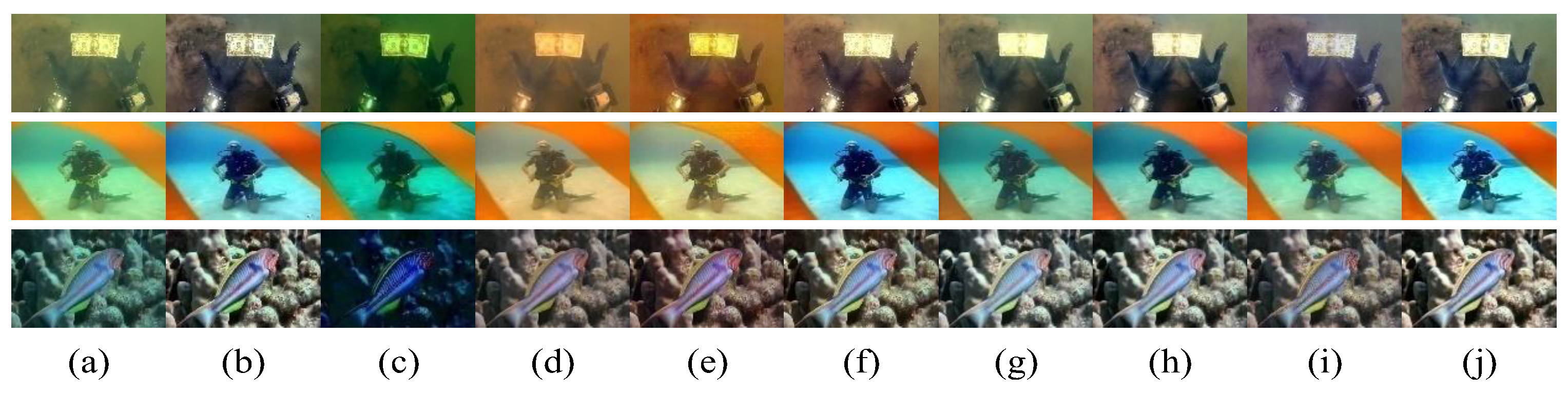
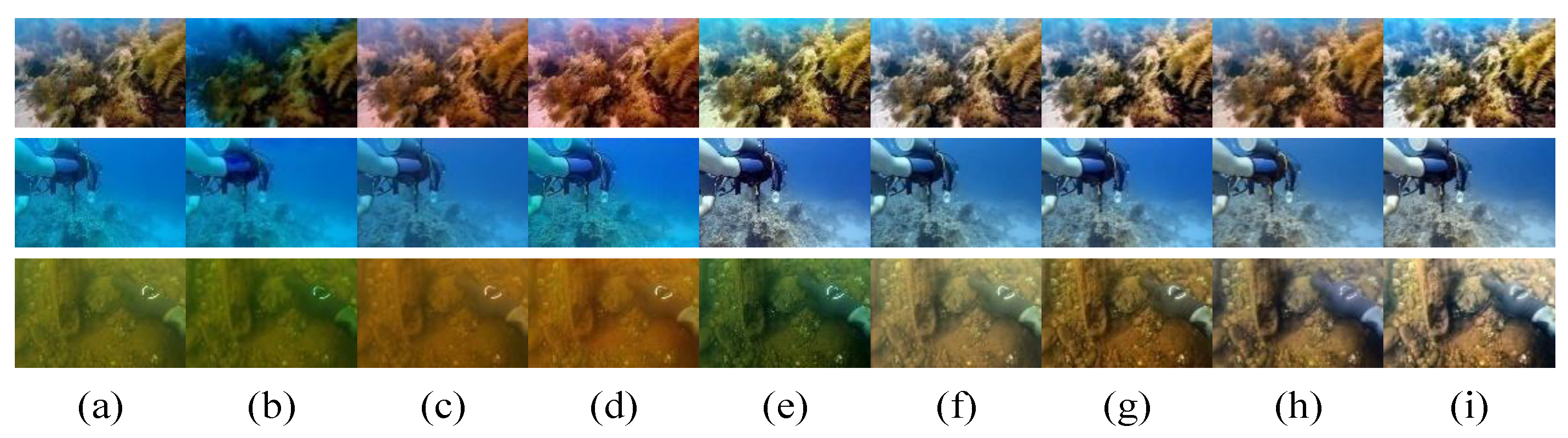
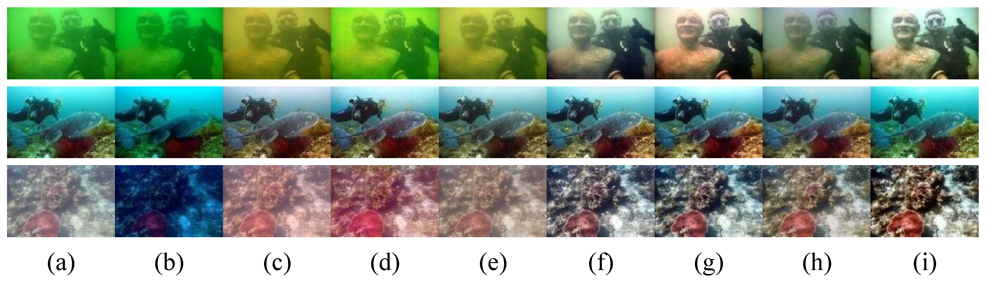
Figure 6 shows results on EUVP-T100. Visually, DCP suffers from severe color cast and distortion. UWNet shows low contrast. FUnIE-GAN restores color and contrast but introduces noise and blur. DeepWaveNet and LitenhanceNet show under-enhancement. LA-Net preserves detail well but struggles with color accuracy in some areas. In contrast, UCA-Net and the U-shape Transformer achieve the best color fidelity and structural detail, performing robustly under challenging underwater conditions.
Figure 7 shows qualitative results on EUVP-R50. DCP exhibits severe color cast with poor enhancement. UWNet and DeepWaveNet correct color moderately but cause blurring and texture loss. FUnIE-GAN introduces artifacts, degrading visual quality. LitenhanceNet under-enhances, with blur and detail loss. LA-Net tends to over-enhance colors, leading to unnatural results. U-shape Transformer performs well but struggles with green attenuation in some cases. In contrast, UCA-Net restores natural colors while preserving textures and details, yielding the best perceptual quality.
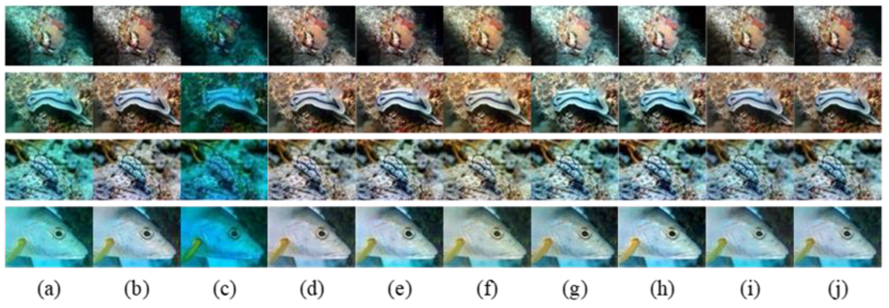
Figure 8 illustrates results on UIEB-T90. DCP performs poorly in both color and detail. UWNet and FUnIE-GAN show yellow over-enhancement due to blue-green suppression. LitenhanceNet and LA-Net under-enhance, but LA-Net better preserves contrast and white balance. U-shape Transformer fails to recover fine details in blurry scenes. UCA-Net and DeepWaveNet produce the best results, though DeepWaveNet still loses saturation and detail.
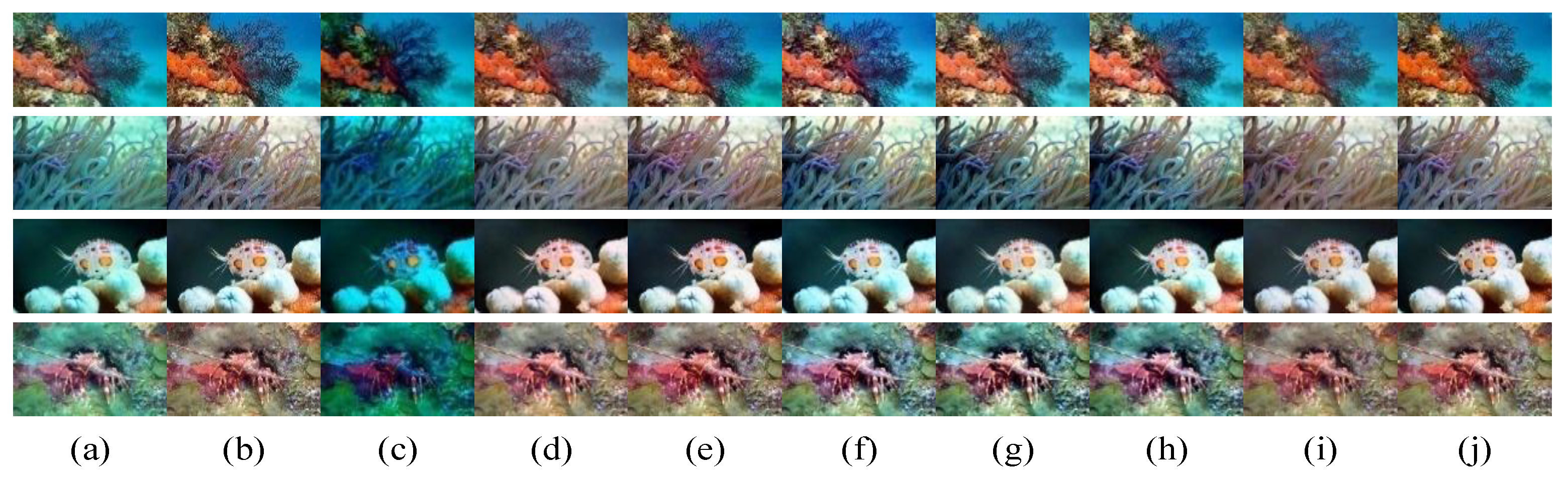
Figure 9 shows results on UIEB-R60. DCP and UWNet fail in color correction, reducing brightness. FUnIE-GAN enhances better but over-amplifies red tones (e.g., first image). DeepWaveNet shows unnatural color balance in challenging scenes (e.g., third image). LitenhanceNet, LA-Net, and U-shape Transformer produce good results but suffer from reduced contrast and noise, causing blur. Overall, LitenhanceNet and UCA-Net perform best, offering balanced enhancement with natural colors and preserved details.
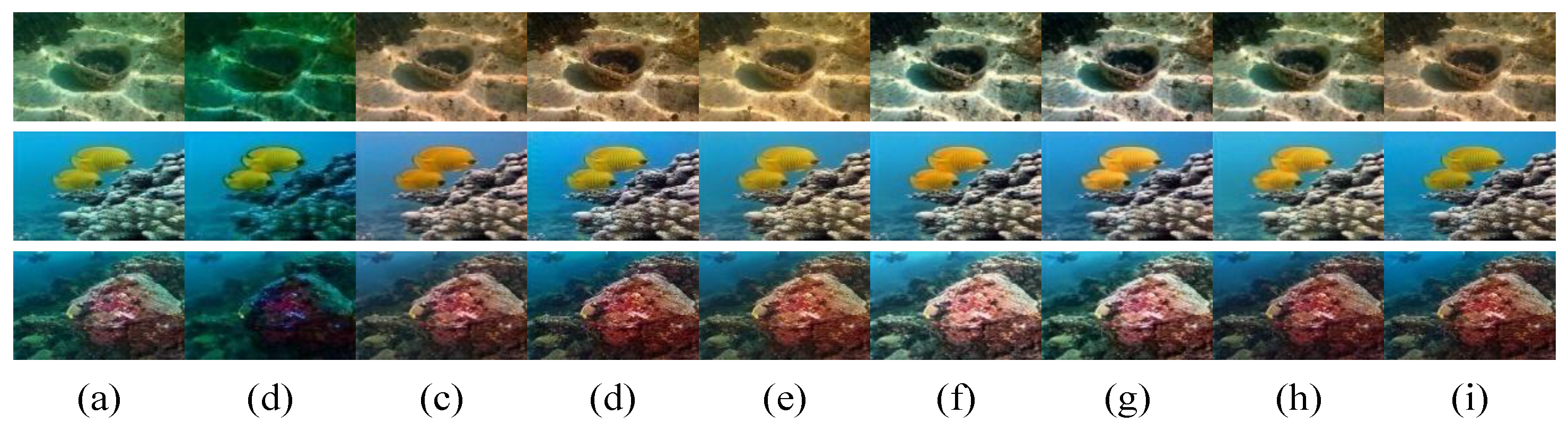
Figure 10 shows results on UFO-T120. DCP introduces color cast and artifacts, degrading visual quality. DeepWaveNet, LitenhanceNet, and LA-Net fail to correct blue-green deviations (e.g., third image). UWNet enhances well overall but lacks accurate white balance and detail preservation. U-shape Transformer restores color moderately but misses fine details. FUnIE-GAN and UCA-Net deliver the best results, achieving superior color fidelity and texture retention.
Figure 11 shows results on LSUI-T100. DCP yields poor enhancement, with major color and clarity deviation. UWNet and FUnIE-GAN improve some aspects but cause yellow tint and color distortion. DeepWaveNet restores color better but blurs details. U-shape Transformer shows white balance errors, leading to inaccurate colors. In contrast, UCA-Net and other top methods balance color correction and detail preservation well, suppressing artifacts. UCA-Net achieves the most natural and visually pleasing results.
Figure 12 shows results on U45. Input images suffer from severe color distortion and blur. DCP fails to correct these, leaving color cast and artifacts. UWNet improves color slightly but does not reduce blur. FUnIE-GAN and DeepWaveNet suppress green poorly and over-enhance red (e.g., third image). LitenhanceNet, LA-Net, and U-shape Transformer improve color but retain blur and introduce noise, causing detail loss. In contrast, UCA-Net achieves the best color and sharpness restoration, effectively handling underwater degradation and preserving fine details.
4.6. Quantitative Comparison
We conducted a quantitative comparison on four benchmark datasets: EUVP-T100, UIEB-T90, UFO-T100, and LSUI-T100. As shown in
Table 1, we report the average PSNR and SSIM for each method. These datasets offer reliable ground-truth references for quantitative evaluation. Results show that traditional methods underperform due to limitations of handcrafted priors. Among deep learning methods, UCA-Net ranks first or second on all datasets, indicating balanced performance in fidelity and perceptual quality. These results align with the qualitative analysis in
Figure 5,
Figure 7,
Figure 9, and
Figure 10, confirming the strength of UCA-Net in color, texture, and detail enhancement.
We conducted no-reference evaluations on EUVP-R50, UIEB-R60, and U45 using UIQM, UCIQE, and CCF (
Table 2), which assess color, contrast, and sharpness. Among eight methods, UCA-Net maintained balanced performance. Though it showed visual superiority in qualitative comparisons, it did not consistently lead in all metrics due to the heuristic nature of these scores, which may misalign with human perception in complex scenes. On EUVP-R50, UCA-Net scored 2.98 (UIQM) and 0.606 (UCIQE), indicating good quality. It achieved top UIQM and UCIQE on UIEB-R60, confirming its effectiveness. Notably, UCA-Net’s UCIQE varied little across datasets, suggesting stable performance under diverse underwater conditions.
4.7. Detailed Functional Evaluation
In this section, we validate the effectiveness of UCA-Net from two perspectives: color fidelity and detail preservation.
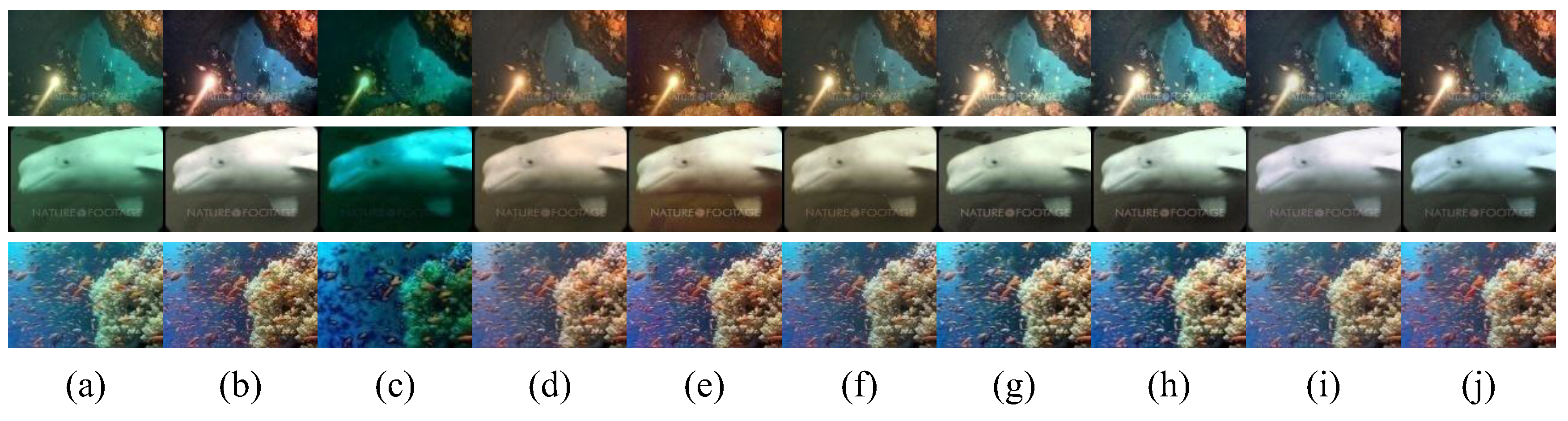
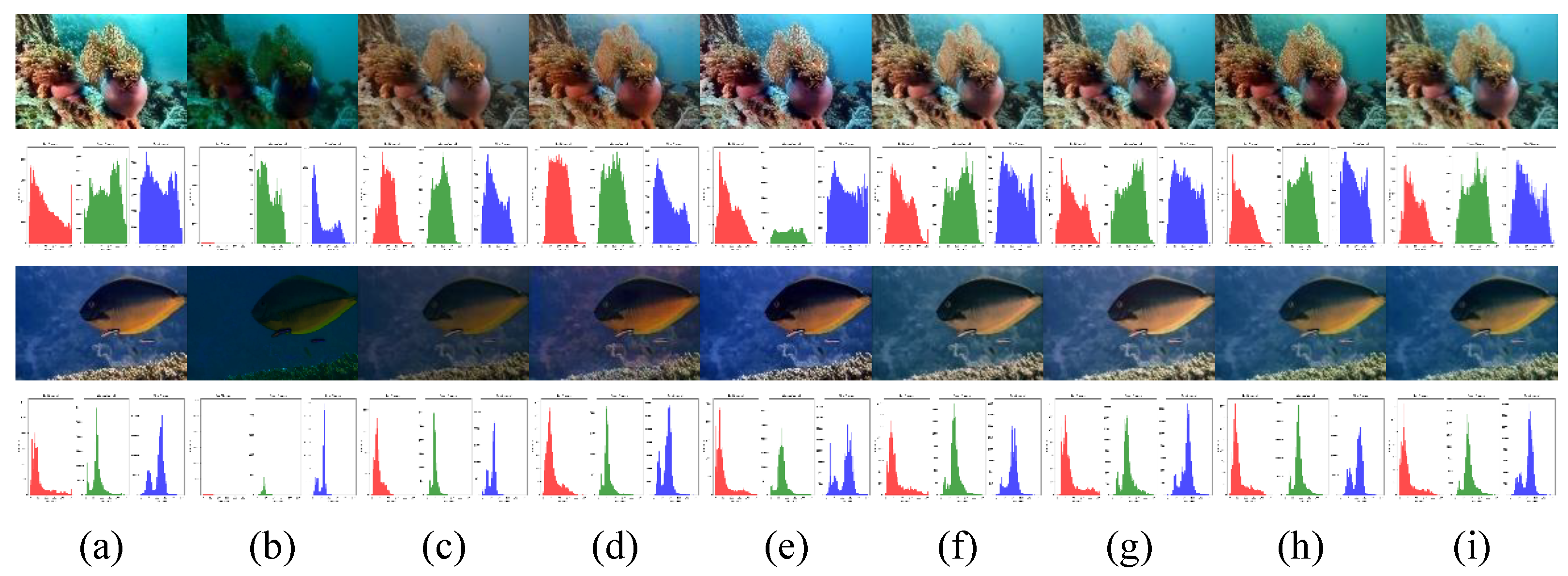
As shown in
Figure 13, we compare color histograms of reference and enhanced images from UIEB. UCA-Net shows the best color alignment, with distributions closely matching the ground truth, indicating effective natural color restoration under underwater distortions.
In
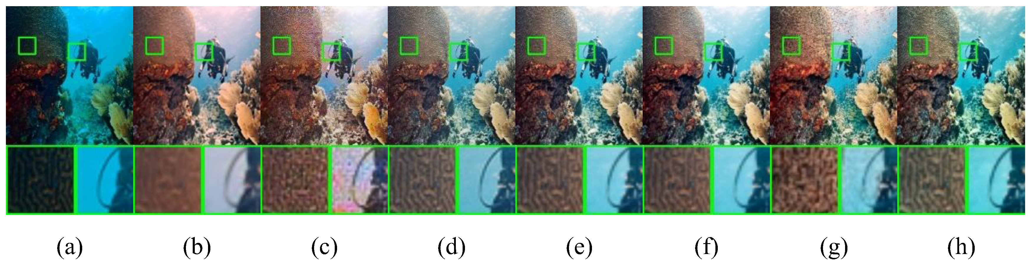
Figure 14, we evaluate texture restoration by zooming into regions of enhanced UIEB images. DCP degrades texture during color adjustment. UWNet produces over-smoothed results lacking depth. FUnIE-GAN fails to maintain structure in complex regions. U-shape Transformer misses fine textures, leading to blurry outputs. In contrast, UCA-Net preserves fine details and edges, achieving sharp, natural enhancements even in challenging conditions.
4.8. Ablation Research
To further verify the effectiveness of the proposed modules in UCA-Net, we conducted a comprehensive ablation study. All experiments were performed on the UIEB dataset, with UIEB-T90 used as the test set. The evaluation was based on two full-reference metrics: PSNR and SSIM.
Table 3 presents the results, comparing performance across multiple model variants, each with one specific component removed or altered. The results validate the importance and contribution of each module to the network’s overall performance in underwater image enhancement. The specific experiments are as follows:
1) No.1: “w/o DCRAC” indicates that DCRAC has been removed.
2) No.2: “w/o DCTB” indicates that DCTB has been removed.
3) No.3: “w/o ADSB” indicates that ADSB has been removed.
4) No.4: “w/o CAM” indicates that CAM has been removed.
5) No.8: “w/o DC” indicates that the deformable convolution in DCTB has been replaced by a regular convolution.
6) No.9: “w/o FDFM” indicates that FDFM has been replaced by simple per-pixel addition.
7) No.9: Loss Function Experiment.
As shown in
Table 3, the full UCA-Net achieves PSNR 24.75 and SSIM 0.89 on UIEB-T90. Removing the DCRAC module drops PSNR by 1.13 and SSIM by 0.11, confirming its effectiveness in reducing noise and enhancing local details via residual convolution and composite attention. Removing ADSB lowers PSNR by 1.12 and SSIM by 0.05, highlighting its role in global color and illumination adjustment. Excluding CAM yields PSNR 24.53 and SSIM 0.81, showing its importance for texture and spatial consistency. Replacing deformable convolutions in DCTB causes performance degradation, proving their benefit for handling irregular underwater textures. Removing FDFM also weakens the results, validating its necessary role in feature fusion targeting global versus local features. These results validate the architectural design of UCA-Net, and each module is crucial to improve the quality.
In
Table 4, ablation on the loss function shows perceptual loss has the greatest impact when removed. L1 and SSIM loss show minor effects, especially under equal weighting. Optimal results occur when α₁ = 0.2, α₂ = 0.2, and α₃ = 1, indicating perceptual loss should dominate.
4.9. Downstream Visual Applications
To verify the specific application effects of our method on image enhancement, we applied it to object detection and image segmentation tasks.
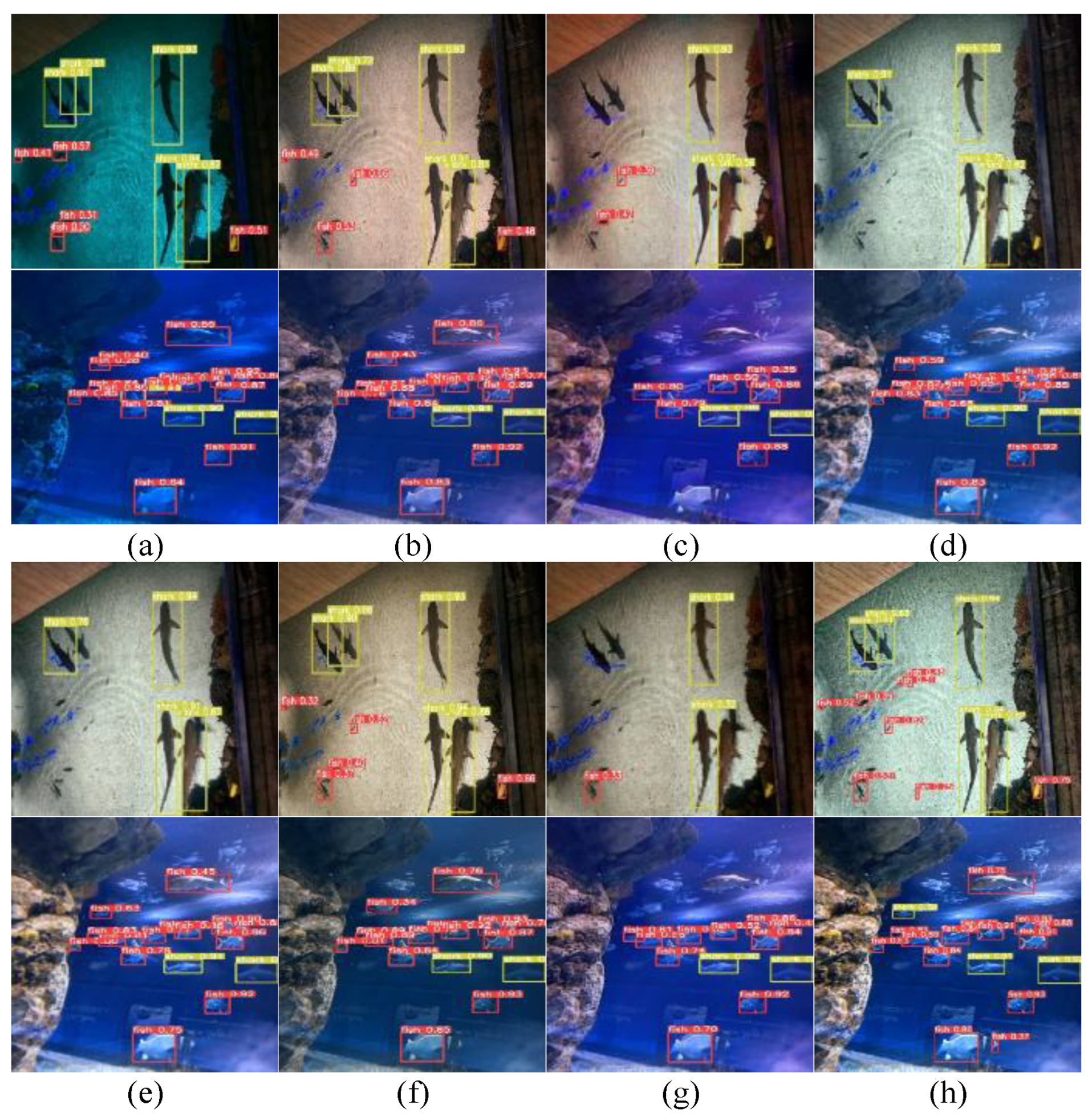
In the object detection task, we trained YOLOv553 on the Aquarium dataset. As shown in
Figure 15, test images with detection metrics allow visual comparison across seven methods. DCP suffers from strong color bias, missing small targets. UWNet and FUnIEGAN over-enhance red, while LitenhenceNet and LA-Net introduce noise and degrade details, leading to missed detections. In contrast, our method detects small, blurred, and low-contrast targets more effectively.
For semantic segmentation, we trained U-Net51 on SUIM52.
Figure 16 shows segmentation results with labeled objects. DCP produces greenish bias, hindering edge detection. UWNet and DeepWaveNet cause color turbidity, impairing accuracy. LA-Net and U-shape Transformer result in occasional overexposure and missegmentation. Our method preserves color and edge features better, supporting more accurate segmentation.
4.10. Complexity Comparison
Model complexity is measured by parameter count (Params) and Multiply-Accumulate Operations (MACs)54. We compared these across methods (
Table 5). Though our model has higher complexity than traditional CNNs, it outperforms other self-attention-based models in both metrics. This shows UCA-Net achieves a lightweight yet effective design, balancing performance and efficiency.
5. Conclusion
We propose UAC-Net, a CNN-Transformer hybrid integrating multiple attention mechanisms. It features an Adaptive Sparse Attention Module (ADSB) with deformable convolution-based residuals to enhance global features for underwater color and light correction. A Composite Attention Module combines three complementary attentions to refine fine details. The parallel dual-attention design jointly handles global and local restoration, addressing distortion and texture loss. The frequency domain feature fusion mechanism organically fused and outputted the output results of parallel attention in the frequency domain. Comparative and ablation studies confirm that UAC-Net consistently outperforms existing methods in both image quality and detail recovery.
Despite strong results, UAC-Net’s lightweight structure can be further optimized. Future work will explore physics-based priors, hardware acceleration, and structural refinement to enhance efficiency and practicality.
Author Contributions
methodology, software, data curation, writing—original draft preparation, Cheng Yu.; validation, Jian Zhou, Guizhen Liu. and Lin Wang.; investigation, Jian Zhou.; resources, Zhongjun Ding.; writing—review and editing, Cheng Yu, Jian Zhou.; supervision, Jian Zhou, Lin ang.; All authors have read and agreed to the published version of the manuscript.
Funding
This research received no external funding.
Data Availability Statement
We encourage all authors of articles published in MDPI journals to share their research data. In this section, please provide details regarding where data supporting reported results can be found, including links to publicly archived datasets analyzed or generated during the study. Where no new data were created, or where data is unavailable due to privacy or ethical restrictions, a statement is still required. Suggested Data Availability Statements are available in section “MDPI Research Data Policies” at
https://www.mdpi.com/ethics.
Conflicts of Interest
The authors declare no conflicts of interest. The funders had no role in the design of the study; in the collection, analyses, or interpretation of data; in the writing of the manuscript; or in the decision to publish the results.
Abbreviations
The following abbreviations are used in this manuscript:
| DCRAC |
Depthwise Separable Convolutional Residual Attention Composite Block |
| DCTB |
Deformable Convolution-Transformer Block |
| FDFM |
Frequency-Domain Feature Fusion Module |
| PTCHM |
Parallel Transformer-CNN Hybrid Module |
| ADSB |
Adaptive Dual-path Self-Attention Block |
References
- Zhou J-c Zhang, D.-h.; Zhang, W.-s. Classical and state-of-the-art approaches for underwater image defogging: a comprehensive survey. Front Inform Technol Electron Eng 2020, 21, 1745–1769. [Google Scholar] [CrossRef]
- Liu, J.; Li, S.; Zhou, C.; Cao, X.; Gao, Y.; Wang, B. SRAF-Net: A Scene-Relevant Anchor-Free Object Detection Network in Remote Sensing Images. IEEE Transactions on Geoscience and Remote Sensing 2022, 60, 5405914. [Google Scholar] [CrossRef]
- Huang, Z.; Wan, L.; Sheng, M.; Zou, J.; Song, J. An underwater image enhancement method for simultaneous localization and mapping of autonomous underwater vehicle. in Proc. 3rd Int. Conf. Robot. Automat. Sci., 2019, pp. 137–142.
- Marengo, M.; Durieux, E.D.H.; Marchand, B.; Francour, P. A review of biology, fisheries and population structure of Dentex dentex (Sparidae). Reviews in Fish Biology and Fisheries 2014, 24, 1065–1088. [Google Scholar] [CrossRef]
- Li, C.-Y.; Guo, J.-C.; Cong, R.-M.; Pang, Y.-W.; Wang, B. Underwater image enhancement by dehazing with minimum information loss and histogram distribution prior. IEEE Trans. Image Process. 2016, 25, 5664–5677. [Google Scholar] [CrossRef] [PubMed]
- Fazal, S.; Khan, D. (2021). Underwater Image Enhancement Using Bi- Histogram Equalization with Fuzzy Plateau Limit. 2021 7th International Conference on Signal Processing and Communication (ICSC), 261–266.
- Ding, X.; Wang, Y.; Zhang, J.; Fu, X. Underwater image dehaze using scene depth estimation with adaptive color correction. in Proc. OCEANS, Jun. 2017, pp. 1–5.
- Chen, L.; Jiang, Z.; Tong, L.; et al. Perceptual underwater image enhancement with deep learning and physical priors. IEEE Transactions on Circuits and Systems for Video Technology 2020, 31, 3078–3092. [Google Scholar] [CrossRef]
- Han, K.; Wang, Y.; Chen, H.; Chen, X.; Guo, J.; Liu, Z.; Tang, Y.; Xiao, A.; Xu, C.; Xu, Y.; Yang, Z.; Zhang, Y.; Tao, D. A Survey on Vision Transformer. IEEE Transactions on Pattern Analysis and Machine Intelligence 2023, 45, 87–110. [Google Scholar] [CrossRef]
- Hitam, M.S.; Awalludin, E.A.; Yussof, W.N.J.H.W.; Bachok, Z. Mixture contrast limited adaptive histogram equalization for underwater image enhancement. in Proc. Int. Conf. Comput. Appl. Technol. (ICCAT), Jan. 2013, pp. 1–5.
- Zhang, W.; Jin, S.; Zhuang, P.; Liang, Z.; Li, C. Underwater image enhancement via piecewise color correction and dual prior optimized contrast enhancement. IEEE Signal Process. Lett. 2023, 30, 229–233. [Google Scholar] [CrossRef]
- Ancuti, C.; Ancuti, C.O.; Haber, T.; et al. (2012). Enhancing underwater images and videos by fusion, In 2012 IEEE conference on computer vision and pattern recognition. IEEE, 2012: 81-88.
- Zhang, S.; Wang, T.; Dong, J.; et al. Underwater image enhancement via extended multi-scale Retinex. Neurocomputing 2017, 245, 1–9. [Google Scholar] [CrossRef]
- Drews, J.; Nascimento, E.; Moraes, F.; Botelho, S.; Campos, M. Transmission estimation in underwater single images. in Proc. IEEE Int. Conf. Comput. Vis. (ICCV) Workshops, Jun. 2013, pp. 825–830.
- Galdran, A.; Pardo, D.; Picon, A.; Alvarez-Gila, A. Automatic redchannel underwater image restoration. Visual Communication and Image Representation, vol. 26, pp. 132–145, Jan. 2014.
- Li, C.-Y.; Guo, J.-C.; Cong, R.-M.; Pang, Y.-W.; Wang, B. Underwater image enhancement by dehazing with minimum information loss and histogram distribution prior. IEEE Trans. Image Process. 2016, 25, 5664–5677. [Google Scholar] [CrossRef]
- Peng, Y.-T.; Cosman, P.C. Underwater image restoration based on image blurriness and light absorption. IEEE Trans. Image Process. 2017, 26, 1579–1594. [Google Scholar] [CrossRef]
- Galdran, A.; Pardo, D.; Picón, A.; Alvarez-Gila, A. Automatic redchannel underwater image restoration. J. Vis. Commun. Image Representation 2015, 26, 132–145. [Google Scholar]
- Li, C.; Anwar, S.; Porikli, F. Underwater scene prior inspired deep underwater image and video enhancement. Pattern Recognition 2020, 98, 107038. [Google Scholar] [CrossRef]
- Naik, A.; Swarnakar, A.; Mittal, K. Shallow-uwnet: Compressed model for underwater image enhancement (student abstract). In AAAI Conference on Artificial Intelligence, pages 15853–15854, 2021.
- Sharma, P.; Bisht, I.; Sur, A. Wavelength-based Attributed Deep Neural Network for Underwater Image Restoration. ACM Transactions on Multimedia Computing, Communications, and Applications 2023, 19, 1–23. [Google Scholar] [CrossRef]
- Qi, Q.; Zhang, Y.; Tian, F.; Wu, Q.J.; Li, K.; Luan, X.; Song, D. Underwater image co-enhancement with correlation feature matching and joint learning. IEEE Transactions on Circuits and Systems for Video Technology 2021, 32, 1133–1147. [Google Scholar] [CrossRef]
- Yang, M.; Hu, K.; Du, Y.; Wei, Z.; Sheng, Z.; Hu, J. Underwater image enhancement based on conditional generative adversarial network. Signal Processing: Image Communication 2020, 81, 115723. [Google Scholar] [CrossRef]
- Islam, M.J.; Xia, Y.; Sattar, J. Fast underwater image enhancement for improved visual perception. IEEE Robotics and Automation Letters 2020, 5, 3227–3234. [Google Scholar] [CrossRef]
- Li, C.; Guo, J. Underwater image enhancement by dehazing and color correction. Journal of Electronic Imaging 2015, 24, 033023. [Google Scholar] [CrossRef]
- Chen, L.; Jiang, Z.; Tong, L.; et al. Perceptual underwater image enhancement with deep learning and physical priors. IEEE Transactions on Circuits and Systems for Video Technology 2020, 31, 3078–3092. [Google Scholar] [CrossRef]
- Liu, Z.; Lin, Y.; Cao, Y.; Hu, H.; Wei, Y.; Zhang, Z.; Lin, S.; Guo, B. (2021). Swin Transformer: Hierarchical Vision Transformer using Shifted Windows. 2021 IEEE/CVF International Conference on Computer Vision (ICCV), 9992–10002.
- Qu, J.; Cao, X.; Jiang, S.; You, J.; Yu, Z. UIEFormer: Lightweight Vision Transformer for Underwater Image Enhancement. IEEE Journal of Oceanic Engineering 2025, 50, 851–865. [Google Scholar] [CrossRef]
- Ren, T.; et al. Reinforced Swin-Convs Transformer for Simultaneous Underwater Sensing Scene Image Enhancement and Super-resolution. IEEE Transactions on Geoscience and Remote Sensing 2022, 60, 1–16. [Google Scholar] [CrossRef]
- Liang, Y.; Li, L.; Zhou, Z.; Tian, L.; Xiao, X.; Zhang, H. Underwater Image Enhancement via Adaptive Bi-Level Color-Based Adjustment. IEEE Trans. Instrumentation and Measurement 2025, 74, 1–16. [Google Scholar] [CrossRef]
- Johnson, J.; Alahi, A.; Fei-Fei, L. Perceptual losses for real-time style transfer and super-resolution. in Proc. 14th Eur. Conf. Comput. Vis., Amsterdam, The Netherlands, 2016, pp. 694–711.
- Li, C.; et al. An underwater image enhancement benchmark dataset and beyond. IEEE Trans. Image Process. 2019, 29, 4376–4389. [Google Scholar] [CrossRef] [PubMed]
- Islam, M.J.; Xia, Y.; Sattar, J. Fast underwater image enhancement for improved visual perception. IEEE Robotics and Automation Letters 2020, 5, 3227–3234. [Google Scholar] [CrossRef]
- Islam, M.J.; Luo, P.; Sattar, J. Simultaneous enhancement and superresolution of underwater imagery for improved visual perception. In 16th Robotics: Science and Systems, RSS 2020, 2020.
- Peng, L.; Zhu, C.; Bian, L. U-shape transformer for underwater image enhancement. IEEE Trans. Image Process. 2023, 32, 3066–3079. [Google Scholar] [CrossRef] [PubMed]
- Li, C.; Guo, C.; Ren, W.; et al. An underwater image enhancement benchmark dataset and beyond. IEEE Transactions on Image Processing 2019, 29, 4376–4389. [Google Scholar] [CrossRef]
- Korhonen, J.; You, J. (2012). Peak signal-to-noise ratio revisited: Is simple beautiful?, In 2012 Fourth International Workshop on Quality of Multimedia Experience. IEEE, 2012: 37-38.
- Wang, Z.; Bovik, A.C.; Sheikh, H.R.; et al. Image quality assessment: from error visibility to structural similarity. IEEE transactions on image processing 2004, 13, 600–612. [Google Scholar] [CrossRef]
- Panetta, K.; Gao, C.; Agaian, S. Human-visual-system-inspired underwater image quality measures. IEEE Journal of Oceanic Engineering 2015, 41, 541–551. [Google Scholar] [CrossRef]
- Yang, M.; Sowmya, A. An underwater color image quality evaluation metric. IEEE Transactions on Image Processing 2015, 24, 6062–6071. [Google Scholar] [CrossRef]
- Wang, Y.; et al. An imaging-inspired no-reference underwater color image quality assessment metric. Comput. Elect. Eng. 2018, 70, 904–913. [Google Scholar] [CrossRef]
- He, K.; Sun, J.; Tang, X. Single Image Haze Removal Using Dark Channel Prior. IEEE Transactions on Pattern Analysis and Machine Intelligence 2011, 33, 2341–2353. [Google Scholar]
- Naik, A.; Swarnakar, A.; Mittal, K. Shallow-uwnet: Compressed model for underwater image enhancement (student abstract). In AAAI Conference on Artificial Intelligence, pages 15853–15854, 2021.
- Islam, M.J.; Xia, Y.; Sattar, J. Fast underwater image enhancement for improved visual perception. IEEE Robotics and Automation Letters 2020, 5, 3227–3234. [Google Scholar] [CrossRef]
- Sharma, P.; Bisht, I.; Sur, A. Wavelength-based attributed deep neural network for underwater image restoration. ACM Transactions on Multimedia Computing, Communications and Applications 2023, 19, 123. [Google Scholar]
- Zhang, S.; Zhao, S.; An, D.; Li, D.; Zhao, R. Liteenhancenet: A lightweight network for real-time single underwater image enhancement. Expert Systems with Applications 2024, 240, 122546. [Google Scholar]
- Liu, S.; Fan, H.; Lin, S.; Wang, Q.; Ding, N.; Tang, Y. Adaptive Learning Attention Network for Underwater Image Enhancement. in IEEE Robotics and Automation Letters 2022, 7, 5326–5333. [Google Scholar]
- Peng, L.; Zhu, C.; Bian, L. U-shape transformer for underwater image enhancement. IEEE Trans. Image Process. 2023, 32, 3066–3079. [Google Scholar] [CrossRef] [PubMed]
- Simonyan, K.; Zisserman, A. Very deep convolutional networks for large-scale image recognition. arXiv 2014, arXiv:1409.1556. [Google Scholar]
- Ashish Vaswani, Noam Shazeer, Niki Parmar, Jakob Uszkoreit, Llion Jones, Aidan N Gomez, Łukasz Kaiser, and Illia Polosukhin. Attention is all you need. In NeurIPS, 2017.
- Ronneberger, O.; Fischer, P.; Brox, T. U-Net: Convolutional networks for biomedical image segmentation. in Proc. 18th Int. Conf. Med. Image Comput. Computer-Assisted Intervention 2015, pp. 234–241. [CrossRef]
- Islam, M.J.; et al. Semantic Segmentation of Underwater Imagery: Dataset and Benchmark. In Proceedings of the 2020 IEEE/RSJ International Conference on Intelligent Robots and Systems (IROS), Las Vegas, NV, USA; 2020; pp. 1769–1776. [Google Scholar]
- Cheng, T.; Song, L.; Ge, Y.; Liu, W.; Wang, X.; Shan, Y. YOLO-world: Real-time open-vocabulary object detection. In Proceedings of the IEEE/CVF Conf. Comput. Vis. Pattern Recognit. (CVPR), Jun. 2024; pp. 16901–16911. [Google Scholar]
- Justus, D.; Brennan, J.; Bonner, S.; McGough, A.S. Predicting the Computational Cost of Deep Learning Models. In Proceedings of the 2018 IEEE International Conference on Big Data (Big Data), Seattle, WA, USA; 2018; pp. 3873–3882. [Google Scholar]
Figure 2.
Schematic diagram of the Composite Attention Module (CAM).
Figure 2.
Schematic diagram of the Composite Attention Module (CAM).
Figure 3.
(a)Schematic diagram of the deformable convolution principle. (b) Structure diagram of deformable convolution.
Figure 3.
(a)Schematic diagram of the deformable convolution principle. (b) Structure diagram of deformable convolution.
Figure 5.
Schematic diagram of the Frequency-Domain Feature Fusion Module (FDFM).
Figure 5.
Schematic diagram of the Frequency-Domain Feature Fusion Module (FDFM).
Figure 6.
Visual comparison results of different methods on the EUVP-T100 test set. (a)input images. (b)reference images. (c)-(i) Results obtained by DCP, UWNet, FUnIEGAN, DeepWaveNet, LitenhencedNet, LA-Net, U-shape Transformer (j)ours.
Figure 6.
Visual comparison results of different methods on the EUVP-T100 test set. (a)input images. (b)reference images. (c)-(i) Results obtained by DCP, UWNet, FUnIEGAN, DeepWaveNet, LitenhencedNet, LA-Net, U-shape Transformer (j)ours.
Figure 7.
Visual comparison results of different methods on the EUVP-R60 test set. (a)input images. (b)-(h) Results obtained by DCP, UWNet, FUnIEGAN, DeepWaveNet, LitenhencedNet, LA-Net, U-shape Transformer (i)ours.
Figure 7.
Visual comparison results of different methods on the EUVP-R60 test set. (a)input images. (b)-(h) Results obtained by DCP, UWNet, FUnIEGAN, DeepWaveNet, LitenhencedNet, LA-Net, U-shape Transformer (i)ours.
Figure 8.
Visual comparison results of different methods on the UIEB-T90 test set. (a)input images. (b)reference images. (c)-(i) Results obtained by DCP, UWNet, FUnIEGAN, DeepWaveNet, LitenhencedNet, LA-Net, U-shape Transformer (j)ours.
Figure 8.
Visual comparison results of different methods on the UIEB-T90 test set. (a)input images. (b)reference images. (c)-(i) Results obtained by DCP, UWNet, FUnIEGAN, DeepWaveNet, LitenhencedNet, LA-Net, U-shape Transformer (j)ours.
Figure 9.
Visual comparison results of different methods on the UIEB-R60 test set. (a)input images. (b)-(h) Results obtained by DCP, UWNet, FUnIEGAN, DeepWaveNet, LitenhencedNet, LA-Net, U-shape Transformer (i)ours.
Figure 9.
Visual comparison results of different methods on the UIEB-R60 test set. (a)input images. (b)-(h) Results obtained by DCP, UWNet, FUnIEGAN, DeepWaveNet, LitenhencedNet, LA-Net, U-shape Transformer (i)ours.
Figure 10.
Visual comparison results of different methods on the UFO-T120 test set. (a)input images. (b)reference images. (c)-(i) Results obtained by DCP, UWNet, FUnIEGAN, DeepWaveNet, LitenhencedNet, LA-Net, U-shape Transformer (j)ours.
Figure 10.
Visual comparison results of different methods on the UFO-T120 test set. (a)input images. (b)reference images. (c)-(i) Results obtained by DCP, UWNet, FUnIEGAN, DeepWaveNet, LitenhencedNet, LA-Net, U-shape Transformer (j)ours.
Figure 11.
Visual comparison results of different methods on the LSUI-T100 test set. (a)input images. (b)reference images. (c)-(i) Results obtained by DCP, UWNet, FUnIEGAN, DeepWaveNet, LitenhencedNet, LA-Net, U-shape Transformer (j)ours.
Figure 11.
Visual comparison results of different methods on the LSUI-T100 test set. (a)input images. (b)reference images. (c)-(i) Results obtained by DCP, UWNet, FUnIEGAN, DeepWaveNet, LitenhencedNet, LA-Net, U-shape Transformer (j)ours.
Figure 12.
Visual comparison results of different methods on the U45 test set. (a)input images. (b)-(h) Results obtained by DCP, UWNet, FUnIEGAN, DeepWaveNet, LitenhencedNet, LA-Net, U-shape Transformer (i)ours.
Figure 12.
Visual comparison results of different methods on the U45 test set. (a)input images. (b)-(h) Results obtained by DCP, UWNet, FUnIEGAN, DeepWaveNet, LitenhencedNet, LA-Net, U-shape Transformer (i)ours.
Figure 13.
Visual comparison of the color histograms of the enhanced images on different comparison methods. (a)Reference images. (b)-(h) Results obtained by DCP, UWNet, FUnIEGAN, DeepWaveNet, LitenhencedNet, LA-Net, U-shape Transformer (i)ours.
Figure 13.
Visual comparison of the color histograms of the enhanced images on different comparison methods. (a)Reference images. (b)-(h) Results obtained by DCP, UWNet, FUnIEGAN, DeepWaveNet, LitenhencedNet, LA-Net, U-shape Transformer (i)ours.
Figure 14.
The detailed magnification and visual comparison of the enhanced image on different comparison methods. (a)-(g) Results obtained by DCP, UWNet, FUnIEGAN, DeepWaveNet, LitenhencedNet, LA-Net, U-shape Transformer (h)ours.
Figure 14.
The detailed magnification and visual comparison of the enhanced image on different comparison methods. (a)-(g) Results obtained by DCP, UWNet, FUnIEGAN, DeepWaveNet, LitenhencedNet, LA-Net, U-shape Transformer (h)ours.
Figure 15.
Detect underwater targets through different methods of YOLOv5. (a)-(g) Results obtained by DCP, UWNet, FUnIEGAN, LitenhencedNet, LA-Net, DeepWaveNet, U-shape Transformer (h)ours.
Figure 15.
Detect underwater targets through different methods of YOLOv5. (a)-(g) Results obtained by DCP, UWNet, FUnIEGAN, LitenhencedNet, LA-Net, DeepWaveNet, U-shape Transformer (h)ours.
Figure 16.
The segmentation tasks of the images enhanced by different methods were compared using Deeplabv3. (a)-(g) Results obtained by DCP, UWNet, FUnIEGAN, LitenhencedNet, LA-Net, DeepWaveNet, U-shape Transformer (h)ours.
Figure 16.
The segmentation tasks of the images enhanced by different methods were compared using Deeplabv3. (a)-(g) Results obtained by DCP, UWNet, FUnIEGAN, LitenhencedNet, LA-Net, DeepWaveNet, U-shape Transformer (h)ours.
Table 1.
Quantitative comparisons of all reference indicators were conducted on the four test sets of EUVP-T100, UIEB-T90, UFO-T100, and LSUI-T100. The red and blue numbers respectively represent the best and sub-best results.
Table 1.
Quantitative comparisons of all reference indicators were conducted on the four test sets of EUVP-T100, UIEB-T90, UFO-T100, and LSUI-T100. The red and blue numbers respectively represent the best and sub-best results.
| Dataset |
Metric |
DCP |
UWNet |
FUnIEGAN |
DeepWaveNet |
LitenhencedNet |
LA-Net |
U-shape Trans |
Ours |
| EUVP-T100 |
PSNR |
13.85 |
25.82 |
25.96 |
25.42 |
20.69 |
21.09 |
24.01 |
27.41 |
| SSIM |
0.48 |
0.74 |
0.78 |
0.81 |
0.74 |
0.75 |
0.75 |
0.86 |
| UIEB-T90 |
PSNR |
14.69 |
18.03 |
19.59 |
22.89 |
23.03 |
23.51 |
21.90 |
24.75 |
| SSIM |
0.67 |
0.71 |
0.72 |
0.82 |
0.87 |
0.88 |
0.82 |
0.89 |
| UFO-T120 |
PSNR |
14.82 |
25.21 |
25.83 |
20.79 |
20.24 |
21.03 |
24.13 |
26.86 |
| SSIM |
0.58 |
0.75 |
0.77 |
0.74 |
0.73 |
0.74 |
0.76 |
0.85 |
| LSUI-T100 |
PSNR |
15.60 |
24.76 |
25.89 |
26.75 |
21.69 |
21.18 |
25.28 |
27.26 |
| SSIM |
0.64 |
0.82 |
0.84 |
0.88 |
0.83 |
0.83 |
0.84 |
0.87 |
Table 2.
All reference indicators were quantitatively compared on three sets of test devices, namely EUVP-R50, UIEB-R60 and U45. The red and blue numbers respectively represent the best and sub-best results, while the green one is the third result.
Table 2.
All reference indicators were quantitatively compared on three sets of test devices, namely EUVP-R50, UIEB-R60 and U45. The red and blue numbers respectively represent the best and sub-best results, while the green one is the third result.
| Dataset |
Metric |
DCP |
UWNet |
FUnIEGAN |
DeepWaveNet |
LitenhencedNet |
LA-Net |
U-shape Trans |
Ours |
| EUVP-R50 |
UIQM |
1.54 |
3.03 |
2.92 |
3.12 |
3.03 |
3.01 |
3.07 |
2.98 |
| UCIQE |
0.571 |
0.585 |
0.594 |
0.592 |
0.619 |
0.620 |
0.591 |
0.606 |
| CCF |
0.088 |
0.989 |
0.839 |
0.997 |
0.824 |
0.823 |
0.833 |
0.895 |
| UIEB-R60 |
UIQM |
1.40 |
2.63 |
3.02 |
2.78 |
2.98 |
2.98 |
3.04 |
3.12 |
| UCIQE |
0.573 |
0.568 |
0.589 |
0.608 |
0.603 |
0.611 |
0.581 |
0.615 |
| CCF |
0.206 |
1.087 |
1.081 |
0.856 |
0.859 |
0.867 |
0.891 |
0.929 |
| U45 |
UIQM |
1.56 |
2.79 |
3.05 |
2.89 |
3.31 |
3.28 |
3.25 |
3.19 |
| UCIQE |
0.539 |
0.528 |
0.559 |
0.533 |
0.583 |
0.601 |
0.567 |
0.604 |
| CCF |
0.066 |
1.015 |
0.892 |
0.951 |
0.823 |
0.864 |
0.852 |
0.880 |
Table 3.
The quantitative results of the network structure ablation study based on the average PSNR and SSIM values of the UIEB dataset.
Table 3.
The quantitative results of the network structure ablation study based on the average PSNR and SSIM values of the UIEB dataset.
| Setting |
Detail |
UIEB-T90 |
| PSNR/SSIM |
|---|
| Full model |
- |
24.75 / 0.89 |
| No.1 |
w/o DCRAC |
23.62 / 0.78 |
| No.2 |
w/o DCTB |
23.57 / 0.82 |
| No.3 |
w/o ADSB |
23.63 / 0.90 |
| No.4 |
w/o CAM |
24.53 / 0.81 |
| No.5 |
w/o DC |
24.60 / 0.85 |
| No.6 |
w/o FDFM |
24.32 / 0.86 |
Table 4.
The quantitative results of the loss function ablation study based on the average PSNR and SSIM values of the UIEB dataset.
Table 4.
The quantitative results of the loss function ablation study based on the average PSNR and SSIM values of the UIEB dataset.
| Loss |
UIEB-T90 |
| PSNR/SSIM |
|---|
| L1 Loss |
22.63 / 0.81 |
| SSIM Loss |
22.82 / 0.80 |
| Perceptual Loss |
23.15 / 0.83 |
| L1 + SSIM |
23.48 / 0.86 |
| L1 + Perceptual |
24.61 / 0.79 |
| SSIM + Perceptual |
24.55 / 0.83 |
| L1 + SSIM + Perceptual |
24.42 / 0.84 |
| 0.5L1 + 0.3SSIM + Perceptual |
24.51 / 0.87 |
| 0.3L1 + 0.1SSIM + Perceptual |
24.58 / 0.89 |
| 0.2L1 + 0.2SSIM + Perceptual |
24.75 / 0.89 |
Table 5.
Comparison of the complexity of different methods.
Table 5.
Comparison of the complexity of different methods.
| Method |
#Params(M) |
#MACS(G) |
| UWNet |
0.22 |
21.71 |
| FUnIEGAN |
7.02 |
10.76 |
| LitenhencedNet |
0.69 |
0.013 |
| LA-Net |
5.15 |
356.03 |
| DeepWaveNet |
0.27 |
18.18 |
| U-shape Transformer |
31.59 |
310.21 |
| Ours |
1.44 |
19.26 |
|
Disclaimer/Publisher’s Note: The statements, opinions and data contained in all publications are solely those of the individual author(s) and contributor(s) and not of MDPI and/or the editor(s). MDPI and/or the editor(s) disclaim responsibility for any injury to people or property resulting from any ideas, methods, instructions or products referred to in the content. |
© 2025 by the authors. Licensee MDPI, Basel, Switzerland. This article is an open access article distributed under the terms and conditions of the Creative Commons Attribution (CC BY) license (http://creativecommons.org/licenses/by/4.0/).