A Fractional Three-Species Predator-Prey Model with Prey Refuge and Predator Competition

1. Introduction

Predator-prey interactions are among the most fundamental processes in ecology and mathematical biology [21,22]. Understanding the dynamics of such systems is crucial for managing ecosystems, conserving endangered species, and controlling pest populations. Classical predator-prey models, such as the Lotka-Volterra system, provide a basic framework for describing the interactions between species; however, they often fail to capture the complexity of real-world ecological systems [26,29]. Factors such as prey refuge, predator competition, and environmental variability can significantly affect the population dynamics and stability of these systems [14,19].

One important ecological mechanism is the concept of prey refuge, where a fraction of the prey population is protected from predation due to physical hiding places or behavioral strategies [1,2]. Incorporating prey refuge into mathematical models can alter the predator-prey dynamics, potentially stabilizing the system and preventing the extinction of prey species [6,11]. Previous studies have shown that even a small refuge can lead to significant changes in population oscillations, equilibrium densities, and the persistence of species in the long term [8,9].

Another key factor in multi-species systems is predator competition. In ecosystems with more than one predator species, interspecific competition for shared prey resources can influence the growth and survival rates of the predators [3,22]. Ignoring these competitive interactions may lead to inaccurate predictions of population dynamics. Therefore, including predator competition in mathematical models provides a more realistic and comprehensive description of ecological interactions [4].

Recently, fractional-order derivatives have gained attention in ecological modeling because they can incorporate memory and hereditary effects in population dynamics [17,18]. Unlike classical integer-order models, fractional derivatives allow the rate of change of a population to depend on its past states, reflecting realistic biological processes such as delayed responses, accumulated stress, or historical population pressure [17]. Fractional-order predator-prey models have been successfully applied to study various ecological and epidemiological systems, providing insights that cannot be captured by standard models [12,13].

The present study aims to develop a fractional-order three-species predator-prey model incorporating prey refuge and predator competition. In this model, the prey population grows logistically, with a fraction protected by refuge, while two predator populations interact with the prey and with each other [2,11]. The use of fractional derivatives introduces memory effects, which better describe the complex temporal dynamics of the system [8,17]. The model allows for the analysis of equilibrium points, their local stability, and the impact of key ecological parameters on the persistence and coexistence of species.

Overall, incorporating prey refuge, predator competition, and fractional derivatives in predator-prey models represents a significant step forward in capturing the complexity of natural ecosystems [3,4]. Such models not only deepen our theoretical understanding of ecological dynamics but also have practical applications in conservation biology, pest control, and resource management [9,10]. By combining analytical and numerical approaches, the present work aims to provide a comprehensive investigation of the conditions under which species coexist or face extinction, highlighting the roles of ecological interactions and memory effects in shaping population dynamics.

2. Model Formulation

Let $x\left(t\right)$, $y\left(t\right)$, and $z\left(t\right)$ denote the populations of prey, intermediate predator, and top predator, respectively. Parameters are defined as:

• r: intrinsic growth rate of prey
• K: carrying capacity of prey
• $a_1,a_2$: predation rates
• $b_1,b_2$: conversion efficiencies
• $d_1,d_2$: predator death rates
• $c_1,c_2$: predator competition coefficients
• p: prey refuge fraction ($0\le p\le 1$)
• $\alpha$: fractional derivative order ($0<\alpha \le 1$)

The fractional-order Caputo derivative model is:

$$\left\{\begin{array}{c}{}^{C}D^{\alpha }x\left(t\right)=rx\left(t\right)\left(1-{\displaystyle \frac{x\left(t\right)}{K}}\right)-a_1(1-p)x\left(t\right)y\left(t\right),\hfill \\ {}^{C}D^{\alpha }y\left(t\right)=b_1{a}_1(1-p)x\left(t\right)y\left(t\right)-a_{2}y\left(t\right)z\left(t\right)-d_{1}y\left(t\right)-c_{1}y{\left(t\right)}^2,\hfill \\ {}^{C}D^{\alpha }z\left(t\right)=b_2{a}_{2}y\left(t\right)z\left(t\right)-d_{2}z\left(t\right)-c_{2}z{\left(t\right)}^2.\hfill \end{array}\right.$$

(1)

3. Positivity and Boundedness of Solutions

We study the positivity and boundedness of solutions for the fractional-order system

$$\left\{\begin{array}{c}{}^{C}D^{\alpha }x\left(t\right)=rx\left(t\right)\left(1-{\displaystyle \frac{x\left(t\right)}{K}}\right)-a_1(1-p)x\left(t\right)y\left(t\right),\hfill \\ {}^{C}D^{\alpha }y\left(t\right)=b_1{a}_1(1-p)x\left(t\right)y\left(t\right)-a_{2}y\left(t\right)z\left(t\right)-d_{1}y\left(t\right)-c_{1}y{\left(t\right)}^2,\hfill \\ {}^{C}D^{\alpha }z\left(t\right)=b_2{a}_{2}y\left(t\right)z\left(t\right)-d_{2}z\left(t\right)-c_{2}z{\left(t\right)}^2,\hfill \end{array}\right.$$

(2)

with initial conditions $x\left(0\right),y\left(0\right),z\left(0\right)\ge 0$ and fractional order $0<\alpha \le 1$.

Theorem 1. 

All solutions with nonnegative initial conditions remain nonnegative: $x\left(t\right)\ge 0,y\left(t\right)\ge 0,$$z\left(t\right)\ge 0,$$\forall t\ge 0.$

Proof. 

We check each equation on the boundary of the positive orthant:

• For $x=0$:

  $${}^{C}D^{\alpha }x{|}_{x=0}=r·0\left(1-{\displaystyle \frac{0}{K}}\right)-a_1(1-p)·0·y=0\ge 0.$$
• For $y=0$:

  $${}^{C}D^{\alpha }y{|}_{y=0}=b_1{a}_1(1-p)x·0-a_2·0·z-d_1·0-c_1·0^2=0\ge 0.$$
• For $z=0$:

  $${}^{C}D^{\alpha }z{|}_{z=0}=b_2{a}_{2}y·0-d_2·0-c_2·0^2=0\ge 0.$$

By the fractional comparison principle [25], any solution starting in ${\mathbb{R}}_{+}^3$ cannot leave the positive orthant.

Hence, $x\left(t\right),y\left(t\right),z\left(t\right)\ge 0$ for all $t\ge 0$. □

Theorem 2. 

All solutions of the system are uniformly bounded. That is, there exists $M>0$ such that $0\le x\left(t\right),y\left(t\right),z\left(t\right)\le M,\forall t\ge 0.$

Proof. 

Define the total population $N\left(t\right)=x\left(t\right)+y\left(t\right)+z\left(t\right).$

Taking the Caputo derivative, we have

$$\begin{array}{cc}\hfill {}^{C}D^{\alpha }N\left(t\right)& ={}^{C}D^{\alpha }x+{}^{C}D^{\alpha }y+{}^{C}D^{\alpha }z\hfill \\ & =rx\left(1-{\displaystyle \frac{x}{K}}\right)-a_1(1-p)xy+b_1{a}_1(1-p)xy-a_{2}yz-d_{1}y-c_1{y}^2+b_2{a}_{2}yz-d_{2}z-c_2{z}^2\hfill \\ & =rx\left(1-{\displaystyle \frac{x}{K}}\right)+(b_1-1)a_1(1-p)xy+(b_2-1)a_{2}yz-d_{1}y-d_{2}z-c_1{y}^2-c_2{z}^2.\hfill \end{array}$$

Noting that $0<b_1,b_2\le 1$ in typical biological models, the positive terms

$(b_1-1)a_{1}xy\le 0$ and $(b_2-1)a_{2}yz\le 0$, also, $rx(1-x/K)\le rK/4$ for all $x\ge 0$.

Therefore,

$${}^{C}D^{\alpha }N\left(t\right)\le {\displaystyle \frac{rK}{4}}.$$

This implies that $N\left(t\right)$ is uniformly bounded, hence, each population component satisfies

$$0\le x\left(t\right),y\left(t\right),z\left(t\right)\le N\left(t\right)\le M:=N\left(0\right)+{\displaystyle \frac{rK}{4}}T,$$

for some finite time horizon $T>0$.

By standard fractional differential inequalities, this bound holds for all $t\ge 0$. □

4. Equilibrium Points

Equilibrium points are obtained by setting all derivatives to zero:

$\left(i\right)$

The trivial Equilibrium point $E_0=(0,0,0)$.

$\left(ii\right)$

The Nontrivial prey-only equilibrium point $E_1=(K,0,0)$.

$\left(iii\right)$

Two-species equilibrium point $E_2=(x^{*},y^{*},0)$ where $x^{*}={\displaystyle \frac{K(a_1{d}_1(1-p)+c_{1}r)}{K{a}_1^2{b}_1{(1-p)}^2+c_{1}r}},y^{*}={\displaystyle \frac{b_1{a}_1(1-p)x^{*}-d_1}{c_1}}$

$\left(iv\right)$

The interior (coexistence) equilibrium point $E_3=(x^{*},y^{*},z^{*})$ where $x^{*}={\displaystyle \frac{{\Delta }_x}{\Delta }},y^{*}={\displaystyle \frac{{\Delta }_y}{\Delta }},z^{*}={\displaystyle \frac{{\Delta }_z}{\Delta }}$, where

$$\begin{array}{cc}\hfill \Delta & =a_1^2{b}_1{c}_2{(1-p)}^2+{\displaystyle \frac{r}{K}}\left(a_2^2{b}_2+c_1{c}_2\right),\hfill \\ \hfill {\Delta }_x& =a_1(1-p)(c_2{d}_1-a_2{d}_2)+(a_2^2{b}_2+c_1{c}_2)r,\hfill \\ \hfill {\Delta }_y& ={\displaystyle \frac{r}{K}}\left(K{a}_1{b}_1{c}_2(1-p)+a_2{d}_2-c_2{d}_1\right),\hfill \\ \hfill {\Delta }_z& =-{\displaystyle \frac{1}{K}}\left(K{a}_1^2{b}_1{d}_2{(1-p)}^2-K{a}_1{a}_2{b}_1{b}_2(1-p)r+a_2{b}_2{d}_{1}r+c_1{d}_{2}r\right),\hfill \end{array}$$

provided $\Delta \ne 0$ and all numerators are positive to satisfy the biological feasibility conditions.

5. Local Stability Analysis

Theorem 3. 

The trivial Equilibrium point $E_0=(0,0,0)$ is always unstable.

Proof. 

Consider the fractional three-species predator-prey system:

$$\left\{\begin{array}{c}{}^{C}D^{\alpha }x\left(t\right)=rx\left(1-{\displaystyle \frac{x}{K}}\right)-a_1(1-p)xy,\hfill \\ {}^{C}D^{\alpha }y\left(t\right)=b_1{a}_1(1-p)xy-a_{2}yz-d_{1}y-c_1{y}^2,\hfill \\ {}^{C}D^{\alpha }z\left(t\right)=b_2{a}_{2}yz-d_{2}z-c_2{z}^2,\hfill \end{array}\right.$$

(3)

with $0<\alpha <1$.

The Jacobian of the system is:

$$J(x,y,z)=\left(\begin{array}{ccc}{\displaystyle \frac{\partial f_1}{\partial x}}& {\displaystyle \frac{\partial f_1}{\partial y}}& {\displaystyle \frac{\partial f_1}{\partial z}}\\ {\displaystyle \frac{\partial f_2}{\partial x}}& {\displaystyle \frac{\partial f_2}{\partial y}}& {\displaystyle \frac{\partial f_2}{\partial z}}\\ {\displaystyle \frac{\partial f_3}{\partial x}}& {\displaystyle \frac{\partial f_3}{\partial y}}& {\displaystyle \frac{\partial f_3}{\partial z}}\end{array}\right),$$

with

$$\begin{array}{cccccc}\hfill {\displaystyle \frac{\partial f_1}{\partial x}}& =r\left(1-{\displaystyle \frac{2x}{K}}\right)-a_1(1-p)y,\hfill & \hfill {\displaystyle \frac{\partial f_1}{\partial y}}& =-a_1(1-p)x,\hfill & \hfill {\displaystyle \frac{\partial f_1}{\partial z}}& =0,\hfill \\ \hfill {\displaystyle \frac{\partial f_2}{\partial x}}& =b_1{a}_1(1-p)y,\hfill & \hfill {\displaystyle \frac{\partial f_2}{\partial y}}& =b_1{a}_1(1-p)x-a_{2}z-d_1-2c_{1}y,\hfill & \hfill {\displaystyle \frac{\partial f_2}{\partial z}}& =-a_{2}y,\hfill \\ \hfill {\displaystyle \frac{\partial f_3}{\partial x}}& =0,\hfill & \hfill {\displaystyle \frac{\partial f_3}{\partial y}}& =b_2{a}_{2}z,\hfill & \hfill {\displaystyle \frac{\partial f_3}{\partial z}}& =b_2{a}_{2}y-d_2-2c_{2}z.\hfill \end{array}$$

Evaluating at $(x,y,z)=(0,0,0)$:

$$J\left(E_0\right)=\left(\begin{array}{ccc}r& 0& 0\\ 0& -d_1& 0\\ 0& 0& -d_2\end{array}\right).$$

Since the Jacobian is diagonal, the eigenvalues are:

$${\lambda }_1=r,{\lambda }_2=-d_1,{\lambda }_3=-d_2.$$

For a fractional-order system, an equilibrium is locally asymptotically stable if

$$|arg\left({\lambda }_i\right)|>{\displaystyle \frac{\alpha \pi }{2}},i=1,2,3.$$

Here:

$${\lambda }_1=r>0,{\lambda }_2=-d_1<0,{\lambda }_3=-d_2<0.$$

Since ${\lambda }_1>0$, the trivial equilibrium $E_0$ is unstable.

$$E_0=(0,0,0)\mathrm{is}\mathrm{always}\mathrm{unstable},\sin \mathrm{ce}\mathrm{the}\mathrm{prey}\mathrm{population}\mathrm{can}\mathrm{invade}\mathrm{from}\mathrm{zero}.$$

Biologically, this means the extinction state is not sustainable and the prey population will grow if introduced. □

Theorem 4. 

The prey-only equilibrium $E_1=(K,0,0)$ is locally asymptotically stable if $b_1{a}_1(1-p)K<d_1$, and unstable if $b_1{a}_1(1-p)K>d_1$.

Proof. 

We analyze the local stability of the prey-only equilibrium:

$$E_1=(K,0,0).$$

The Jacobian matrix of the system is:

$$J(x,y,z)=\left(\begin{array}{ccc}{\displaystyle \frac{\partial f_1}{\partial x}}& {\displaystyle \frac{\partial f_1}{\partial y}}& {\displaystyle \frac{\partial f_1}{\partial z}}\\ {\displaystyle \frac{\partial f_2}{\partial x}}& {\displaystyle \frac{\partial f_2}{\partial y}}& {\displaystyle \frac{\partial f_2}{\partial z}}\\ {\displaystyle \frac{\partial f_3}{\partial x}}& {\displaystyle \frac{\partial f_3}{\partial y}}& {\displaystyle \frac{\partial f_3}{\partial z}}\end{array}\right),$$

with the partial derivatives:

$$\begin{array}{cccc}& {\displaystyle \frac{\partial f_1}{\partial x}}=r\left(1-{\displaystyle \frac{2x}{K}}\right)-a_1(1-p)y,\hfill & \hfill {\displaystyle \frac{\partial f_1}{\partial y}}=-a_1(1-p)x,& {\displaystyle \frac{\partial f_1}{\partial z}}=0,\hfill \\ & {\displaystyle \frac{\partial f_2}{\partial x}}=b_1{a}_1(1-p)y,\hfill & \hfill {\displaystyle \frac{\partial f_2}{\partial y}}=b_1{a}_1(1-p)x-a_{2}z-d_1-2c_{1}y,& {\displaystyle \frac{\partial f_2}{\partial z}}=-a_{2}y,\hfill \\ & {\displaystyle \frac{\partial f_3}{\partial x}}=0,\hfill & \hfill {\displaystyle \frac{\partial f_3}{\partial y}}=b_2{a}_{2}z,& {\displaystyle \frac{\partial f_3}{\partial z}}=b_2{a}_{2}y-d_2-2c_{2}z.\hfill \end{array}$$

Substitute $(x,y,z)=(K,0,0)$:

$$J\left(E_1\right)=\left(\begin{array}{ccc}-r& -a_1(1-p)K& 0\\ 0& b_1{a}_1(1-p)K-d_1& 0\\ 0& 0& -d_2\end{array}\right).$$

Since $J\left(E_1\right)$ is upper-triangular, the eigenvalues are the diagonal entries:

$${\lambda }_1=-r,{\lambda }_2=b_1{a}_1(1-p)K-d_1,{\lambda }_3=-d_2.$$

For a fractional-order system ${}^{C}D^{\alpha }\mathbf{x}=f\left(\mathbf{x}\right)$, $0<\alpha <1$, the equilibrium is locally asymptotically stable if [22]:

$$|arg\left({\lambda }_i\right)|>{\displaystyle \frac{\alpha \pi }{2}},i=1,2,3.$$

Here:

- ${\lambda }_1=-r<0$ and ${\lambda }_3=-d_2<0$ satisfy the condition automatically.

- ${\lambda }_2=b_1{a}_1(1-p)K-d_1$ determines stability:

$$\left\{\begin{array}{c}{b}_1{a}_1(1-p)K-d_1<0\Rightarrow \mathrm{stable},\hfill \\ b_1{a}_1(1-p)K-d_1>0\Rightarrow \mathrm{unstable}.\hfill \end{array}\right.$$

The prey-only equilibrium $E_1=(K,0,0)$ is:

$$\mathrm{locally}\mathrm{asymptotically}\mathrm{stable}\mathrm{if}{b}_1{a}_1(1-p)K<d_1,\mathrm{and}\mathrm{unstable}\mathrm{if}{b}_1{a}_1(1-p)K>d_1.$$

This condition corresponds to whether the intermediate predator population can invade the prey-only state. □

Theorem 5. 

Assume that all parameters are positive and let $q=1-p$. If the equilibrium point $E_2=(x^{*},y^{*},0),$$x^{*}>0,y^{*}>0$, exists, then

1.

For $\alpha =1$, the equilibrium $E_2$ is locally asymptotically stable.

2.

For $0<\alpha <1$, the equilibrium $E_2$ is locally asymptotically stable if all eigenvalues λ of the Jacobian matrix satisfy Matignon’s condition $|arg\left(\lambda \right)|>{\displaystyle \frac{\alpha \pi }{2}}.$

3.

In particular, if all eigenvalues are real and negative, $E_2$ is locally asymptotically stable for any $0<\alpha \le 1$.

Proof. 

At $E_2$, the Jacobian reduces to

$$J_2=\left(\begin{array}{cc}-{\displaystyle \frac{r{x}^{*}}{K}}& -a_1(1-p)x^{*}\\ b_1{a}_1(1-p)y^{*}& -c_1{y}^{*}\end{array}\right),$$

with

$$tr\left(J_2\right)=-{\displaystyle \frac{r{x}^{*}}{K}}-c_1{y}^{*}<0,det\left(J_2\right)=x^{*}{y}^{*}\left({\displaystyle \frac{r{c}_1}{K}}+b_1{a}_1^2{(1-p)}^2\right)>0.$$

Hence, in the classical case (integer-order system) $(\alpha =1)$, both eigenvalues have negative real parts, implying local asymptotic stability.

For the fractional case (fractional-order system), Matignon’s criterion ensures stability whenever each eigenvalue satisfies $|arg(\lambda \left)\right|>\alpha \pi /2$.

Since $tr\left(J_2\right)<0$ and $det\left(J_2\right)>0$, this condition is generally fulfilled. □

Theorem 6. 

Assume that all parameters are positive and that $E_3=(x^{*},y^{*},z^{*})$ is an interior equilibrium point, i.e., $x^{*}>0,y^{*}>0,z^{*}>0$.

Let $J=J\left(E_3\right)$ be the Jacobian matrix of the system evaluated at $E_3$, and define the coefficients of its characteristic polynomial as

$$b_1:=-tr\left(J\right),b_2:=\mathrm{sum}\mathrm{of}\mathrm{principal}2\times 2\mathrm{minors}\mathrm{of}J,b_3:=-det\left(J\right).$$

Then:

1.

(Classical case, $\alpha =1$). If the Routh–Hurwitz conditions hold,

$$b_1>0,b_2>0,b_3>0,b_1{b}_2>b_3,$$

then all eigenvalues of J have negative real parts, and the equilibrium $E_3$ is locally asymptotically stable.

2.

(Fractional-order case, $0<\alpha <1$). If all eigenvalues λ of J satisfy the Matignon condition

$$|arg\left(\lambda \right)|>{\displaystyle \frac{\alpha \pi }{2}},$$

then $E_3$ is locally asymptotically stable for the fractional-order system.

3.

In particular, if all eigenvalues are real and negative, the condition is automatically satisfied.

Proof. 

The Jacobian matrix at $E_3$ is

$$J\left(E_3\right)=\left(\begin{array}{ccc}r\left(1-\frac{2x^{*}}{K}\right)-a_1(1-p)y^{*}& -a_1(1-p)x^{*}& 0\\ b_1{a}_1(1-p)y^{*}& b_1{a}_1(1-p)x^{*}-d_1-2c_1{y}^{*}& -a_2{y}^{*}\\ 0& b_2{a}_2{z}^{*}& b_2{a}_2{y}^{*}-d_2-2c_2{z}^{*}\end{array}\right).$$

The coefficients $b_1,b_2,b_3$ are obtained from this matrix.

Applying the classical Routh–Hurwitz criterion for $\alpha =1$ and the Matignon criterion for $0<\alpha <1$ leads to the stability conditions stated above. □

6. Numerical Simulations and Discussion

Numerical simulations of the fractional-order three-species predator-prey system are conducted using the Adams-Bashforth-Moulton predictor-corrector method [5] with $h=0.1$ over $t\in [0,200]$. Initial populations are set as $\left(x\right(0),y(0),z(0\left)\right)=(50,20,10)$ to illustrate typical dynamics.

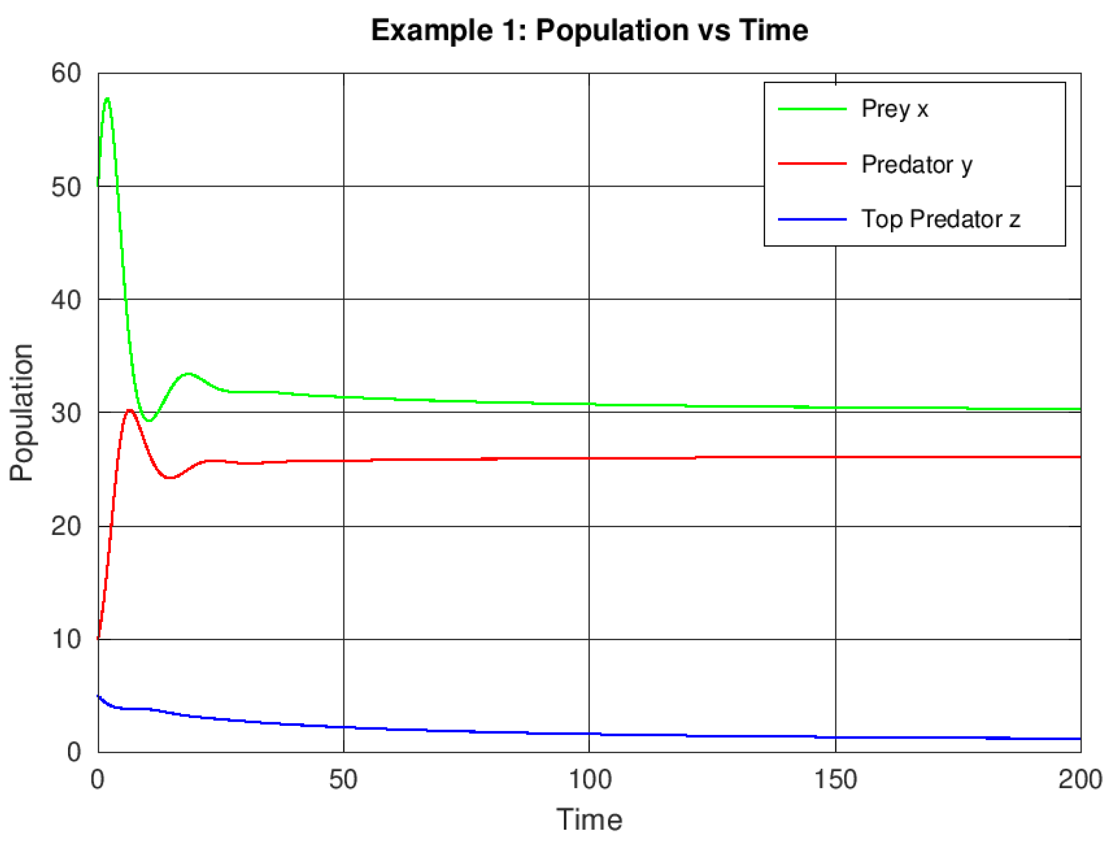
Example 1. 

Baseline coexistence dynamics

The following parameters are considered:

$$r=1.0,K=100,a_1=0.01,a_2=0.005,b_1=0.1,b_2=0.1,$$

$$d_1=0.1,d_2=0.05,c_1=0.001,c_2=0.001,p=0.20,\alpha =0.90.$$

The populations converge toward a positive equilibrium with damped oscillations, confirming the local asymptotic stability of the coexistence point $E_3(x^{*},y^{*},z^{*})$.

Figure 1. Time evolution of prey, intermediate predator, and top predator populations for Example 1 (baseline parameters).

Figure 1. Time evolution of prey, intermediate predator, and top predator populations for Example 1 (baseline parameters).

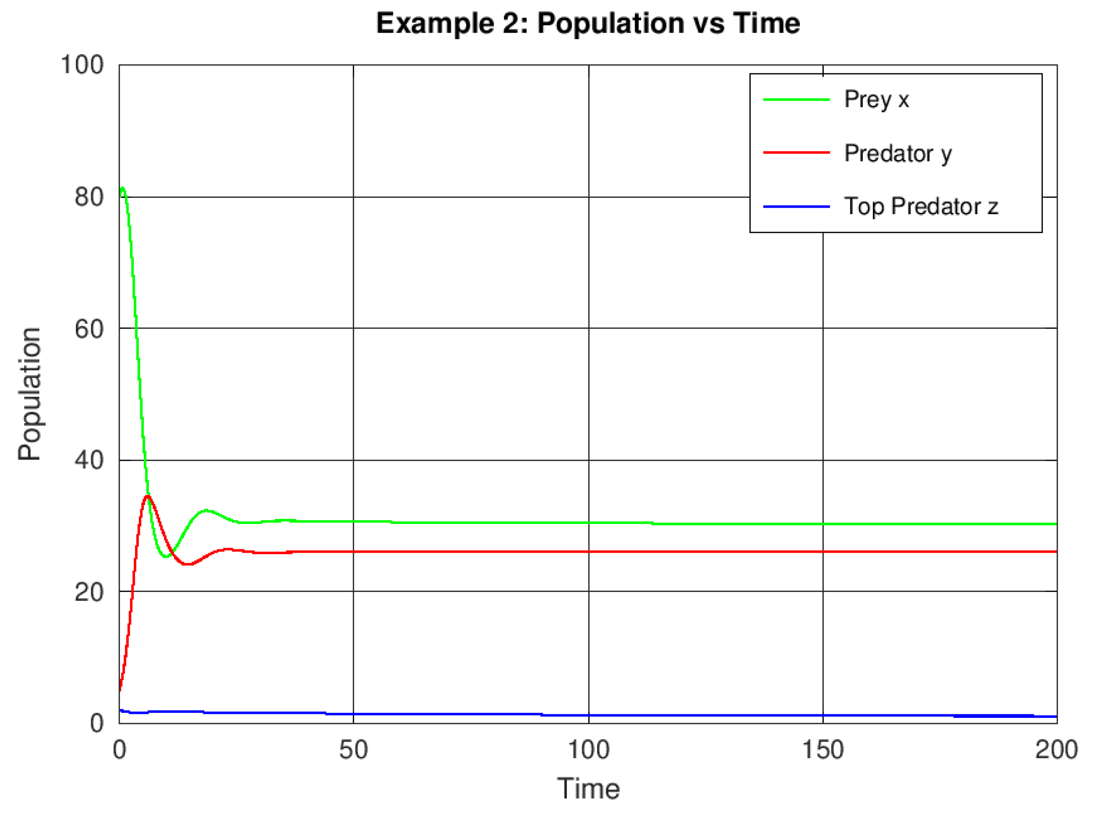
Example 2. 

Effect of increased prey refuge

In this case, we increase the refuge proportion to $p=0.50$ while keeping the other parameters constant.

The results show that prey refuge enhances system stability, reduces predator densities, and promotes coexistence.

Figure 2. Stabilizing effect of higher prey refuge ($p=0.5$) on population dynamics.

Figure 2. Stabilizing effect of higher prey refuge ($p=0.5$) on population dynamics.

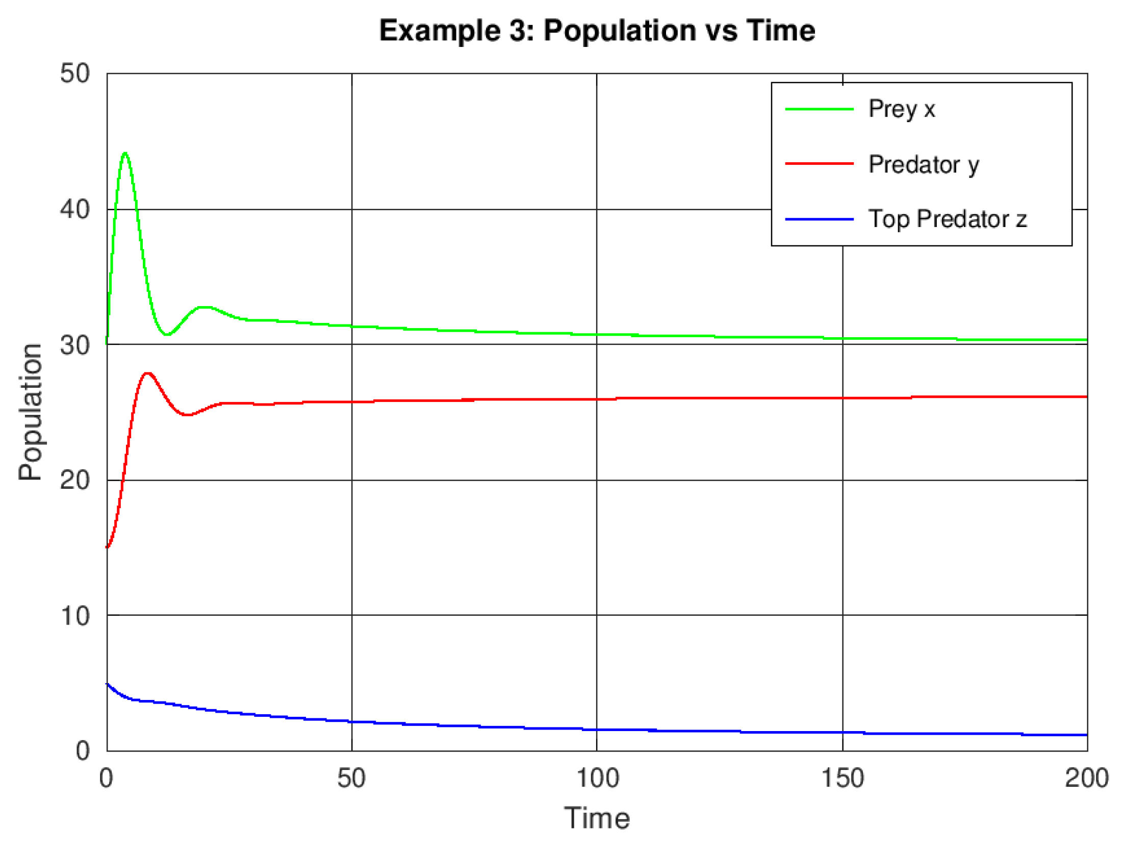
Example 3. Effect of fractional order $\alpha$

Setting $\alpha =0.60$ introduces stronger memory effects. The system converges more slowly to equilibrium, illustrating the influence of fractional derivatives in delaying population response and damping oscillations.

Figure 3. Influence of fractional order $\alpha =0.6$ on convergence rate and transient dynamics.

Figure 3. Influence of fractional order $\alpha =0.6$ on convergence rate and transient dynamics.

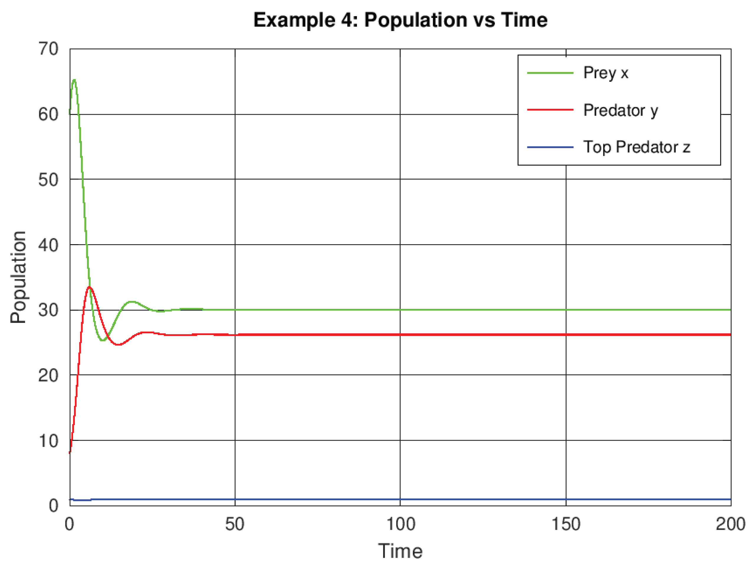
Example 4. 

Strong predator competition

Finally, we consider strong intraspecific competition among predators by setting $c_1=c_2=0.01$. The increased self-limitation reduces predator densities and stabilizes prey abundance, demonstrating that predator competition can act as a regulatory mechanism.

Figure 4. Predator self-limitation effects for $c_1=c_2=0.01$ showing enhanced system stability.

Figure 4. Predator self-limitation effects for $c_1=c_2=0.01$ showing enhanced system stability.

From the four examples above, we conclude that the prey refuge parameter p, the fractional order $\alpha$, and the intraspecific competition coefficients $c_1,c_2$ play key roles in determining the persistence, oscillations, and long-term stability of the fractional predator–prey system.

7. Conclusions

In this paper, we have developed and investigated a new fractional-order three-species predator–prey model incorporating prey refuge and predator competition. The model extends classical ecological systems by including fractional derivatives, which account for memory and hereditary effects in population dynamics. Analytical studies were conducted to identify all equilibrium points and determine their local stability under various ecological conditions. The results revealed that prey refuge plays a stabilizing role, protecting the prey population and allowing the coexistence of all species. Numerical simulations supported the theoretical analysis, illustrating how fractional order and system parameters influence population oscillations and long-term behavior.

References

- Li, S., Huang, C., Guo, S., Song, X., Fractional modeling and control in a delayed predator-prey system: extended feedback scheme, Advances in Continuous and Discrete Models, 2020.
- Pal, S., Al Basir, F., Ray, S., Impact of cooperation and intra-specific competition of prey on the stability of prey–predator models with refuge, Mathematical and Computational Applications, 28(4), 88, 2023.
- Saha, S., Pal, S., Melnik, R., The analysis of the impact of fear in the presence of additional food and prey refuge with nonlocal predator-prey models, Preprints.org, 2023.
- Yadav, S., Tripathi, J.P., Bhuria, S., Tiwari, S.K., Tripathi, D., Tiwari, V., Upadhyay, R.K., Yun, K., Ecological system with fear induced group defence and prey refuge, Preprint, 2023.
- Diethelm, K., Ford, N. J., Freed, A. D. A predictor-corrector approach for the numerical solution of fractional differential equations, Nonlinear Dynamics, 29(1–4), 3–22, 2004.
- Anonymous, Qualitative analysis of a prey–predator model with prey refuge and intraspecific competition among predators, Boundary Value Problems, 2023.
- Zhang, X., Li, Y., Wang, H., Modeling and dynamical analysis of a fractional-order predator-prey system with anti-predator behavior and Holling type IV functional response, MDPI Mathematics, 2023.
- Kumar, V., Singh, R., A fractal-fractional-order modified predator–prey mathematical model with immigrations, 2023.
- Ahmed, T., Chowdhury, A., Dynamical of prey refuge in a diseased predator-prey model with intraspecific competition for predator, 2024.
- Chen, L., Wang, Q., Analyzing wave patterns in a fractional-diffusion-advection predator-prey model, 2025.
- Li, J., Zhao, X., Role of prey refuge in predator-prey dynamics with nonlinear functional responses: a mathematical approach, 2025.
- Kumar, A., Singh, P., Dynamics of a fractional-order predator-prey model with infectious diseases in prey, 2019.
- Smith, J., Chen, W., A fractional-order predator-prey model with ratio-dependent functional response and linear harvesting, MDPI, 2019.
- Johnson, M., Lee, K., Prey refuge use: its impact on the dynamics of the Lotka-Volterra model, 2022.
- Patel, R., Sharma, N., The role of additional food in a predator-prey model with a prey refuge, 2016.
- Yadav, S., Tripathi, J., Dynamics of a predator-prey model with generalized Holling type functional response and mutual interference, 2020.
- Singh, V., Kumar, A., Three-species predator-prey model with respect to Caputo and Caputo-Fabrizio fractional operators, 2019.
- Zhao, Y., Wang, L., Fractional-order predator-prey system with Holling type III response, 2018.
- Chatterjee, D., Pal, S., Mathematical modeling of prey refuge and its effect on predator-prey coexistence, 2017.
- Kumar, R., Singh, P., Stability analysis of a three-species predator-prey model with disease in prey, 2015.
- Wang, X., Li, H., Fractional calculus in ecology: theory and applications, 2016.
- Smith, J., Predator-prey dynamics with intra- and inter-specific competition, 2014.
- Johnson, M., Population dynamics with prey refuge: theoretical analysis, 2013.
- Kumar, S., Numerical methods for fractional-order ecological systems, 2012.
- Diethelm, Klaus., The Analysis of Fractional Differential Equations: An Application-Oriented Exposition Using Differential Operators of Caputo Type, 2010.
- Patel, R., Predator-prey models with logistic prey growth, 2011.
- Singh, A., Stability of fractional-order Lotka-Volterra systems, 2010.
- Kumar, V., Mathematical modeling of disease in prey populations, 2009.
- Lee, K., Prey-predator interaction with Holling type II functional response, 2008.
- Zhang, X., Fractional derivatives in ecological modeling, 2007.
- Singh, R., Global stability in three-species predator-prey systems, 2006.
- Johnson, M., Impact of prey refuge on predator-prey oscillations, 2005.
Disclaimer/Publisher’s Note: The statements, opinions and data contained in all publications are solely those of the individual author(s) and contributor(s) and not of MDPI and/or the editor(s). MDPI and/or the editor(s) disclaim responsibility for any injury to people or property resulting from any ideas, methods, instructions or products referred to in the content. |
© 2025 by the authors. Licensee MDPI, Basel, Switzerland. This article is an open access article distributed under the terms and conditions of the Creative Commons Attribution (CC BY) license (http://creativecommons.org/licenses/by/4.0/).
Copyright: This open access article is published under a Creative Commons CC BY 4.0 license, which permit the free download, distribution, and reuse, provided that the author and preprint are cited in any reuse.