Submitted:
25 November 2025
Posted:
26 November 2025
You are already at the latest version
Abstract
Three-dimensional printing technology for microsensor fabrication is gaining popularity due to its lower cost compared with conventional manufacturing techniques. Such cost reduction is particularly advantageous for the development of affordable devices designed for liquid sensing. Among them, biofuels have emerged as a promising alternative to conventional fuels, offering improved environmental sustainability. Nevertheless, inadequate control of their physicochemical properties can lead to increased emissions and potential engine damage. In this work, we present a sensor system for monitoring biofuel solutions. The device employs piezoelectric sensors integrated with 3D-printed, liquid-filled cells whose structural design is refined through experimental validation and novel optimization strategies that account for sensitivity, recovery, and resolution. The system incorporates discrete electronic circuits and a microcontroller, within which artificial intelligence algorithms are implemented to correlate sensor responses with fluid viscosity and density. The proposed approach achieves calibration and resolution errors as low as 0.99% and 1.48 · 10−2 mPa·s for viscosity, and 0.00485% and 1.9 · 10−4 g/mL for density, enabling detection of small compositional variations in biofuels. Additionally, algorithmic methodologies for dimensionality reduction and data treatment are introduced to address temporal drift, enhance sensor lifespan, and accelerate data acquisition. The resulting system is compact, low-cost, precise, and applicable to diverse industrial liquids.
Keywords:
3D-printing
; sensor
; biofuel
; artificial intelligence
; optimization
; drift
1. Introduction
Three-dimensional (3D) printing enables cost-effective and highly precise sensor manufacturing, positioning it as a good alternative to traditional techniques like lithography and thin-film deposition. In this context, numerous studies have explored the application of 3D-printing technologies in the fabrication of piezoelectric sensors. For instance, in [1,2,3,4,5] they employed polyvinylidene fluoride (PVDF) polymers and their copolymers to develop piezoelectric devices for various sensing applications. These include pressure and force sensors tested under controlled laboratory conditions [1,3], acoustic receivers [4], flow sensors for deionized water, mimicking blood flow [2], and tactile sensors embedded in prosthetic hands capable of identifying object hardness [5]. In [6,7], the authors designed micromachined piezoelectric ultrasonic transducers (PMUTs) using PZT sheets mounted on titanium substrates. These were integrated with Helmholtz resonators featuring 3D-printed cavities of controllable volume to monitor human respiratory patterns. Additional approaches include the use of photopolymer resins mixed with PZT particles to fabricate ultrasonic wave sensors [8], and the development of piezoresistive MEMS accelerometers via 3D-printing for controlled experimental use [9].
A particularly active area of research involves 3D-printed sensors for liquid analysis [10,11,12,13,14]. These works leverage additive manufacturing to produce complete sensor assemblies, fluidic cavities, or microfluidic channels. Sensor modalities include substrate-integrated waveguide (SIW)-based designs [10,15,16], microwave resonators [11,13,14,17,18], parallel plate configurations [12], optical interferometers [19], and electromagnetic bandgap (EBG) microstrip sensors [20]. These systems enabled the differentiation of liquid compositions by measuring dielectric permittivity or transmission spectra. Applications span petroleum monitoring [18]; aqueous mixtures with water-ethanol blends [10,11,12,13,14] being the most notably but also solutions containing isopropanol [15], glucose [19], or potassium chloride [12]; toluene-methanol mixtures [20] and various pure chemicals [13,14,16,17,20]. All aforementioned studies used laboratory instrumentation in the measurement process.
Recent advancements have also integrated machine learning techniques with 3D-printed sensor systems. For example, in [21], the authors developed a deformation-sensitive sensor composed of graphene nanoparticles and carbon nanotubes, employing support vector machines (SVMs) to classify human motion and monitor exhalation; researchers in [22] applied neural networks to optimize the design of a 3D-printed accelerometer for human movement tracking, while in [23] they fabricated 3-axis force sensors and trained a support vector regression (SVR) model on simulated data to quantify forces in medical contexts; finally, the work in [24] combined multi-sensor 3D-printing with machine learning algorithms to predict behavioral impairment following alcohol consumption.
In previous studies [25,26], we introduced a 3D-printed sensing cell incorporating piezoelectric actuators, designed to vibrate at a specific resonance, and artificial intelligence (AI) techniques to characterize the physical properties of aqueous-glycerin solutions. In the present work, we propose an enhanced version of this type of sensor, designed to broaden its operational bandwidth and improve calibration and resolution results. Furthermore, we integrated the sensor into a microcontroller-based system equipped with convolutional neural networks (CNNs), targeting the application of biofuel monitoring. The development of such sensing platforms is particularly relevant given the increasing demand for fuels, their diverse applications, and the need to reduce emissions. Nevertheless, while biofuels are environmentally more favorable, they can lead to elevated emissions or suboptimal engine performance if their viscosity and density are not properly controlled [27,28,29,30]. Numerous studies have explored sensor technologies for monitoring the physical properties of fuels, biofuels and engine oils [29,30,31,32,33,34,35,36,37,38]. More recently, artificial intelligence has become a powerful complement to microsensor technologies, enabling advanced compositional analysis of fuel–lubricant and biofuel mixtures [39,40,41,42]. However, many of these approaches depend on costly instrumentation and complex electronics. To address this limitation, our recent work [43] presented a compact, integrated sensing device. While effective, that design employed a MEMS-based sensor which had higher manufacturing costs. In contrast, the present study focuses on a more cost-effective alternative without compromising performance.
The article is structured as follows: the “Materials and Methods section” details the sensor design, geometric parameters, simulation procedures, structural optimization criteria, complete device schematics, experimental methodology, the data processing techniques and the machine learning algorithms studied. The “Results” section presents optimal sensor geometries identified in real-world applications, experimental data captured with our system from biofuel monitoring, the architecture of the most effective AI models, and their precision obtained in calibration and drift experiments, as well as using dimensionality reduction, compared to the reference values. In the “Discussion”, we contextualize our findings within the existing literature and outline potential future research directions. Finally, we conclude with the key contributions and implications of this work.
2. Materials and Methods
2.1. Comparative Analysis of Sensor Structure and Actuator Layouts
The fundamental architecture of the developed sensor is illustrated in Figure 1. The device comprised two integrated components forming a unified system. The first part consisted of a semi-cylindrical container cell designed to hold the target liquid. This cell featured a vibrating membrane at its base and lateral connectors to facilitate fluid circulation. It was fabricated via stereolithography (SLA) 3D-printing technology [44] using a Formalbs® Form3 printer [44] and Rigid10K resin [45], a material validated in previous studies [25,26] for its mechanical robustness (Young’s modulus = 10 GPa). According to manufacturer specifications [45], this resin also demonstrates good chemical resistance against fuel exposure, exhibiting only a 0.1% weight increase after 24 hours when a sample structure is immersed in diesel. Key printing parameters including dimensional tolerance, resolution, printing speed, and ultraviolet (UV) light exposure duration were controlled throughout the manufacturing process.
The second component comprised the piezoelectric actuators. Commercially available PZT sheets (PIC255, type 5A modified lead zirconate titanate [46]), 100 microns thick, with top and bottom CuNi metallization, and a stiffness of 63 GPa, were manually sectioned and placed on the external surface of the cell membrane using a cyanoacrylate-based contact adhesive (Loctite® 401 [47]). This configuration ensured isolation of the piezoelectric ceramics from the diesel medium, preventing potential chemical degradation. The adhesive selection was validated by previous comparative studies, which revealed negligible performance variation across different cyanoacrylate formulations, attributed to the minimal adhesive layer thickness employed and its relatively low stiffness compared to other structural components of the sensor. Prior to adhesive application, the cell was subjected to an oxygen plasma treatment to improve surface wettability. This process was conducted for 2 minutes at 50 W plasma power and 0.2 mBar oxygen pressure within a vacuum chamber equipped with a radiofrequency plasma generator.
To establish electrical connectivity, 100 Cu wires were soldered to each end of the piezoelectric patches. The opposite ends of the wires were connected to pins embedded in elastomeric plastic tubing for mechanical isolation. The integrity of the solder joints was verified by analyzing the impedance spectrum of the patches across a frequency range of 1 Hz to 1 MHz using an Agilent® 4294A impedance analyzer [48]. These elastomer-coated pins were subsequently inserted into the cell’s side connector protrusions, yielding a compact assembly and minimizing the influence of unwanted variable mechanical coupling caused by the introduction of the cell into a ZIF socket interface for electronic connection.
The optimization of piezoelectric patch configurations was assisted by finite element simulations in COMSOL® Multiphysics [49], enabling a comparative analysis of different actuator layouts based on their spectral response. In contrast, the design of the fluidic cell geometry was addressed experimentally due to the complexity of incorporating full three-dimensional fluid–structure interaction in the model. Multiple prototypes were fabricated and tested under controlled conditions, applying a performance metric focused on resonance amplitude, repeatability, and sensitivity to fluid changes to identify the most suitable sensor architecture.
The geometry and quantity of piezoelectric patches play a critical role in sensor design, as these components, being the most rigid elements, exert a dominant influence on the device’s response. Although simultaneous optimization of the host structure and patch geometry could be addressed as described in [50], this work focuses on a simpler approach: a computational evaluation comparing various actuator configurations to identify the optimal designs. To facilitate this analysis, a simplified cell model was developed using COMSOL. Mechanical and electrical boundary conditions were accurately defined, while non-essential geometric features such as side connectors were excluded due to their less impact on the sensor’s dynamic behavior. A mesh-convergence study was performed to ensure that the finite element results were independent of mesh density while maintaining computational efficiency. Additionally, as previously explained, fluid-structure interactions were omitted to streamline the simulation within a three-dimensional framework. Figure 2 illustrates the piezoelectric patch configurations analyzed through this approach. Performance assessment was based on the voltage amplitude spectrum within the operational frequency range of 1 kHz to 1 MHz. The optimization criterion aimed to maximize both the number and amplitude of resonance peaks in the spectra as these serve as sources of sensor data related to the target liquid [51]. Simulation results indicated that geometries 1 and 6–8 yielded suboptimal spectral profiles. Complementing this analysis, we conducted natural frequency simulations of the standard cell model either with a single piezoelectric sheet on its membrane or with two patches aligned along the vertical axis. In-plane stress values were averaged across all resulting modal shapes, yielding the distribution shown in Figure 3. We can observe that superposition of modes within this frequency range produced low-stress regions at the mid-width and mid-length of the structures, concentrating the effective action and sensing areas in the quadrants. As a result, structures such as 2-4 and 9-10 re-emerged (especially configurations 3, 9 and 10), further reinforcing the previous conclusions. Consequently, we concentrated the fabrication on configurations 2–4 and 9–10, which are also represented in the sensor schematic in Figure 1, with the possible cutouts of actuators highlighted by a black mesh in the plan view.
The other key component is the fluidic container. As previously outlined, one objective of this study was to develop a sensor capable of producing spectral responses characterized by a high number of resonances with high amplitude in a certain frequency range. However, these spectral features must also exhibit sensitivity to fluid changes, maintain repeatability across measurements to attain good resolution, and demonstrate recovery upon reintroduction of the reference fluid. To achieve this, we experimented with the geometric parameters of the fluidic cell depicted in Figure 1. Sensors were fabricated using parameter combinations within the ranges specified in Table 1. Iterative adjustments were made based on comparative performance, with superior parameter values informing the design of subsequent prototypes. This approach enabled progressive refinement of the sensor architecture.
The method for optimizing the cell structure consisted of the following experimental procedure. A sensor fabricated with a given set of geometric parameters was subjected to two fluids via a peristaltic pump: one comprising pure diesel fuel, and the other consisting of a 90:10 volumetric mixture of diesel and commercial sunflower oil. Starting with pure diesel, spectral data were acquired using an Analog Discovery 2 (AD) instrument [52] across a frequency range of 1 kHz to 1 MHz, discretized into 800 points. A sinusoidal input signal of 3.3 V was applied, preceded by a brief stabilization period to ensure fluid equilibrium. For each frequency point, measurements were performed over at least 10 signal periods and were averaged to enhance data robustness. Two spectra were recorded with a time interval of 5 minutes between successive acquisitions. Subsequently, the pure diesel was replaced with the adulterated mixture, using no further cleaning other than the entrainment effect of the new solution. The same measurement protocol was repeated, and finally, the system was flushed with pure diesel once more, and the measurement cycle was repeated. All measurements were conducted under static fluid conditions at room temperature (22±1ºC).
This experimental framework enabled the evaluation of three key performance metrics: sensitivity, reproducibility, and recovery. These were quantified as absolute differences between: spectra of different solutions (); spectra of different consecutive measurements corresponding to the same solution (); spectra of the same fluid measured before and after exposure to a different fluid (). The expression denotes the spectrum corresponding to measurement of liquid j (either pure diesel or the adulterated mixture). A higher sensitivity is desirable, indicating strong differentiation between fluid types, whereas elevated differentiation in resolution or recovery is undesirable, as it reflects inconsistency in repeated measurements of the same fluid.
Based on these definitions, to determine whether greater sensitivity `compensates’ for poorer resolution and recovery at each spectral point i, we propose the following equation. This formulation also serves as a dimensionality reduction strategy for subsequent analysis:
where “max” denotes the greatest difference, corresponding to the worst result between resolution and recovery. To quantify the relative performance of each cell, two metrics are proposed: the first uses equation (1) to compute m over all points of the spectrum and , while the second uses only the points where sensitivity compensates for resolution/recovery () and . Then, in both cases, the mean value across all spectral points is calculated and the sensors with higher values of m are considered the best. The two approaches produced comparable results.
2.2. System Description and Calibration-Drift Experiments
This section presents the architecture of the measurement system designed to operate the sensors optimized using the method described in the preceding subsection, together with the experimental protocol implemented for calibration and drift assessment.
The best sensors were integrated into a measurement system analogous to that depicted in Figure 4, previously introduced in [51] for MEMS-based detection of adulterants in olive oil. In addition to the sensor element, the system comprised electronic interfacing circuits designed to operate with an ESP32-S3-DevKitC-1-N32R8V microcontroller [53]. Fluid samples were introduced into the sensor at maximum flow rate using a Gilson Minipuls 3 peristaltic pump [54]. A transistor-based circuit was employed to amplify the Pulse Width Modulation (PWM) signal generated by the microcontroller, which served to excite the sensor’s input actuator patch(es). The PWM frequency was swept from 10 kHz to 1 MHz, yielding 530 discrete frequency spectra. A variable frequency step was used to account for the microcontroller’s limited frequency resolution. The sensor’s output signal was further amplified via a bipolar junction transistor (BJT) biasing circuit incorporating emitter and collector feedback to improve DC stability at the operating point. This amplified signal was processed by an envelope detector, also implemented using a discrete transistor circuit, and captured via the microcontroller’s analog-to-digital converter (ADC). For each excitation frequency, 1000 output samples were acquired, each comprising 10 response periods. Averaging across these samples improved data robustness. All electronic components were powered using the 5 V supply provided by the microcontroller.
The measurement procedure was repeated for each of the biodiesel solutions listed in Table 2. These solutions were prepared by blending commercial diesel fuel with sunflower oil in proportions consistent with those reported in the literature and compliant with European regulatory standards [28]. The table contains the physical properties of the fluids, determined by averaging three measurements obtained using a commercial Anton Paar DMA4100M densitometer equipped with a Lovis module [55], maintained at 40ºC. Samples were introduced into the system in ascending order of viscosity. For each fluid, measurements were conducted under static conditions following a stabilization period of 5-15 minutes, and subsequently 33 spectra were collected over approximately 10 minutes. When changing the fluid, the sensor was flushed with the incoming fluid for 3 minutes without any additional cleaning protocol. All measurements were performed without active temperature control of the resonator; ambient temperature during the experiments was maintained at 23±1°C. Furthermore, the experiment was repeated using solutions , , and over a period of four days to assess whether spectral variations arising from temporal drift could be mitigated through data processing and AI techniques.
2.3. Deep Learning Algorithms Optimization
Following the acquisition of spectral data from all prepared solutions, machine learning models were constructed to establish predictive relationships between the spectra and the corresponding physical properties of the fluids. As demonstrated in our previous studies [26,43,51], convolutional neural networks exhibit strong performance in the analysis and interpretation of spectral signals. The procedures employed to identify network architectures best suited to our data, together with the spectral drift compensation and dimensionality reduction strategies implemented, are detailed below.
The first step involved defining the data sets and applying appropriate scaling. Mixtures labeled were designated as the training set, whereas mixtures labeled were reserved exclusively for testing and were not used during parameter optimization. Prior to training, the data were preprocessed using a scaling method based on the standard deviation. Following this process, optimization of the neural network architecture was undertaken. To identify the best network configurations that improve predictive accuracy, we applied a hyperparameter fine-tuning strategy analogous to that used in [43,51]. Specifically, we varied the number of convolutional layers (up to five), the number of filters, their size and stride. The tested parameter values are illustrated in Table 3, which summarizes the general architecture of the evaluated models. The filters and their associated parameters define distinct mechanisms for spectral feature extraction. The ReLU activation function was employed to facilitate gradient-based optimization via the Adam algorithm [56], which has proven effective in CNN training. Learning rates ranging from 0.01 to 0.001 were explored to minimize the mean squared error loss function. To control model complexity, we incorporated either high stride values or max-pooling layers, which perform local subsampling by selecting the maximum value within a defined neighborhood. Following the final convolutional block, an average pooling layer was applied to reduce dimensionality, thereby removing the need for a flattening operation and fully connected layers. This design choice is critical, as the latter approach introduces additional parameters and computational overhead, which are incompatible with the constraints of microcontroller deployment. The network ended with a single output neuron using a linear activation function to predict the target physical properties, such as viscosity or density. To identify the most effective model architecture, a comparative evaluation was conducted by quantifying the prediction error. This error was computed as the arithmetic mean of the absolute differences between the model-predicted values of viscosity or density and the corresponding reference values obtained from the commercial laboratory-grade viscometer. This approach enabled the selection of the network configuration that yielded the highest predictive accuracy. All models were implemented and trained using TensorFlow 2.17 [57].
The models were subsequently evaluated using data obtained from drift experiments. To simulate realistic operating conditions, liquid was selected as the reference fluid for measurements on different days. We employed this liquid as a reference because it constitutes a representative solution of the problem under study, namely biodiesels derived from mixtures of conventional diesel and sunflower oil, and it exhibits a comparatively low viscosity relative to other biofuels in our dataset, thereby enabling more efficient removal during the circulation of subsequent liquids to be measured. Following the measurement protocol described earlier, the mean spectrum was calculated from repeated measurements. The ratio between the average spectrum of the reference solution on the initial day (day 0) and that obtained on day n was then determined. This ratio defines a spectral factor , which encodes the relative variations in sensor response between day 0 and day n across all spectral components, each of which may evolve differently over time. The factor was then employed to adjust the spectra of subsequent solutions. Specifically, the adjustment consisted of multiplying the measured spectrum of a given solution by , thereby approximating a transformation of the data from day n back to day 0. The corrected spectrum was then reintroduced as input to the trained machine learning models, yielding more accurate predictions of viscosity and density compared to unprocessed spectra. In this way, the operational lifespan of both the sensor and the overall system can be extended simply by using one single unique calibration solution as reference.
In addition, a dimensionality reduction study was conducted as follows. Using the equation (1) as a basis, the number of spectral points was progressively reduced, thereby decreasing measurement time while simultaneously evaluating the impact on neural network training and performance in both calibration and drift experiments.
It is important to note that the models were trained externally and subsequently deployed on the microcontroller via the TensorFlow Lite library, enabling a fully autonomous viscosity and density monitoring system. This machine learning framework not only enhanced system autonomy but also simplified the electronic requirements for signal processing, because any spurious effect originating from the parasitic elements of the resonator or the electronics remains constant across all measurements, so they can be learned and disregarded by the machine learning models.
3. Results
This section applies the previously defined performance metric to evaluate and compare 64 sensor geometries fabricated during the design refinement process. It presents representative examples illustrating how the criterion guided structural selection, summarizes the final geometric parameters, and discusses the influence of piezoelectric patch distribution and fluidic cell features on overall sensor performance.
In addition, we describe the outcomes of calibration and drift experiments performed with the optimized sensor integrated into the microcontroller-based system. These results include spectral measurements for all prepared solutions, the predictive performance of CNN models for viscosity and density estimation, and their comparison with laboratory references. The section also examines the correction of temporal drift and explores dimensionality reduction as a means to accelerate measurements while preserving accuracy and enabling efficient deployment on resource-constrained hardware.
3.1. Optimization of the Sensor Structure
As described in Section 2, we employed a systematic approach to refine the geometry of the liquid-containing cell, guided by equation 1 and the measurement protocol described in the corresponding subsection. According to this equation, spectral points yielding values greater than 1 are considered positive, as they indicate that the sensor’s sensitivity exceeds its limitations in resolution or recovery. Conversely, values below 1 are regarded as negative, since insufficient resolution or recovery cannot be distinguished from spectral variations induced by changes in the liquid. In total, 64 combinations of geometric parameters were designed, fabricated, and tested. Figure 5 illustrates the application of the optimization method to two representative geometries: one of larger dimensions without fins (left), and another of smaller scale incorporating membrane extensions (right). In the figure, green lines indicate cases where , while red lines correspond to , enabling refinement of the cell structure based on this criterion.
Following the structural refinement process, several conclusions could be drawn:
- In general, miniaturization of the cell, and consequently its patches, yielded improved m-metric values.
- When the cell membrane was fully covered by piezoelectric actuators, the addition of fins produced inferior results compared to an empty configuration. Conversely, when the actuators were reduced in size such that half of the membrane remained uncovered, the presence of fins substantially enhanced the m-metrics relative to a hollow cell.
- A comparable improvement was observed when the membrane thickness was reduced. However, combining fin addition with reduced membrane thickness led to overall poorer performance, as each factor independently increases variability in the printing process, and their simultaneous application amplifies this variability. Accordingly, a thicker membrane proved more suitable when fins were incorporated.
- The optimal fin configuration consisted of one fin per quadrant of the cell (i.e., a 2×2 array). Increasing the number of cilia along either axis degraded performance.
- A reduced arrangement (1×2) produced comparable results only when the cilia were positioned within quadrants.
- Complete coverage of the membrane with four piezoelectric patches significantly worsened the m-metric values, likely due to multiplied defects introduced during fabrication and gluing of the patches.
It should be emphasized that these conclusions are constrained by inherent imperfections in sensor fabrication. Manufacturing processes introduce additional sources of variability, including cell curing, resin evacuation, patch cutting, and non-uniform adhesion. Therefore, the findings presented here should be regarded as design guidelines rather than definitive optimization criteria.
Figure 6 presents the outcomes of these structural refinement techniques. Table 4 summarizes the geometric values obtained for this sensor. Regarding patch components, both vertical and horizontal divisions were observed, as described earlier. For the fluidic cell, a compact design incorporating four internal fins, one per rectangular quadrant, proved sufficient to achieve good results across the three defined metrics, while minimizing material requirements. Notably, alternative models based on this geometry, such as those with a 0.2 mm membrane or without fins, also performed well experimentally.
3.1.1. Calibration and Drift Experiments
The sensor depicted in Figure 6 was integrated into the microcontroller system illustrated in Figure 4. Subsequently, experiments were conducted to measure the solutions listed in Table 2, following the protocol described in subSection 2.2. A total of 363 spectra were acquired, as shown in Figure 7 (a). This figure demonstrates the capability of the proposed system to detect subtle variations in liquid properties.
Based on these data, convolutional neural networks were trained to predict viscosity and density using the optimization procedure explained in subSection 2.3. The solutions labeled N in Table 2 served as training data, while the remaining fluid measurements were reserved for testing, thereby assessing the model’s generalization performance. The optimal network architectures identified for both viscosity and density estimation followed the configuration shown in Figure 7 (b). This architecture comprised three convolutional layers with 8, 16, and 32 filters, respectively, each with a kernel size of 5 and a stride of 5, without intermediate max-pooling layers. The network concluded with a global average pooling layer and a dense output layer containing a single neuron, as detailed in the corresponding subsection. Training was performed with a batch size of 55 over 200 epochs.
Figure 8 (a) and (b) present the results obtained with our predictive models in comparison with the laboratory instrument. In Figure 8 (a), the red boxes denote viscosity predictions for the training solutions (N), the blue boxes correspond to the test solutions (T), and the green dots indicate the reference values measured with the commercial viscometer.
Similarly, Figure 8 (b) shows the density predictions, where the green boxes represent the training set, the orange boxes the test set, and the blue dots the reference measurements. For viscosity, the system successfully distinguishes between pure diesel and a mixture containing 1% sunflower oil; however, minor adulterations remain undetectable, as evidenced by the overlap of boxplot extremes. The density predictions are also very accurate. To further evaluate the system robustness, we repeated the measurement procedure described in subSection 2.2 for fluids , , and over four consecutive days. This experiment enabled the development of an algorithmic approach to extend sensor lifespan. Specifically, the previously trained models were combined with the drift correction method explained in subSection 2.3, yielding the results shown in Figure 8 (c) and (d). These figures compare predictions obtained from spectra recorded on day 0, corresponding to the initial measurement of the 11 solutions, with those derived from spectra collected on subsequent days. Spectral variations attributable to temporal drift were observed, underscoring the need for correction. Although prediction accuracy decreases over time, the integration of the models with the spectral transformation method still permits differentiation among most solutions. This demonstrates that simple algorithmic strategies can effectively mitigate drift effects and extend the operational lifetime of the sensing system, achieving accuracies sufficient for certain practical applications.
Table 5 and Table 6 report the mean errors associated with the viscosity and density models during the calibration experiment, whereas Table 7 and Table 8 present the corresponding results for the drift experiment. Consistent with previous studies [51], several metrics were employed to evaluate model performance: the absolute difference between predicted and reference values ( and ); the ratio between the mean error and the operating range (full-scale error, ); the relative deviation, defined as the mean difference normalized by the reference values (); and the resolution error, quantified as the standard deviation across repeated measurements of the same solution (). The tabulated results corroborate the conclusions observed in the graphics: both calibration and resolution errors are minimal, and when comparing drift experiment outcomes with those obtained on day 0, the errors increase slightly but remain within acceptable limits.
Finally, a dimensionality reduction analysis was performed using metric 1, using the new definition of resolution as the standard deviation, with the objective of reducing data acquisition time and thereby accelerating the estimation of fluid physical properties. To this end, progressively fewer spectral points were selected according to equation 1, and new convolutional neural networks were trained following the protocol described in subSection 2.3. The trained models were applied both to the calibration experiment and to the drift experiment. Table 9, Table 10, Table 11 and Table 12 summarize the errors obtained. The results indicate that performance remains comparable whether 530 or 103 spectral points are used, demonstrating that measurement time can be reduced with minimal impact on accuracy. Moreover, reducing the input dimensionality to 103 points lowered computational demands; that is, the optimal neural networks contained fewer parameters, improving their suitability for implementation in the limited memory of microcontrollers. Figure 9 presents the graphical results obtained with models trained on spectra of 103 points, confirming their strong overall performance when compared with models trained on spectra of 530 points (Figure 8).
4. Discussion
Using the error values reported in the tables of the previous section, the performance of the proposed device can be compared with that of other viscosity and density monitoring systems described in the literature [25,26,31,32,33,35,36,43]. The results of this comparison are presented in Table 13 and Table 14. For viscosity measurements, the proposed system achieves the second-best performance in the and metrics, ranking only behind [43], while in the metric it occupies the third position (after [33] and [43]). In terms of density, the accuracy of our system consistently ranks third across the , and metrics. With respect to resolution, the device ranks close to fourth, corresponding to the results reported by [43]. It should be emphasized that the studies compiled here are not restricted to fuels; they also encompass other types of liquids, whose interactions with the sensor material may yield either improved or diminished monitoring performance. A particularly relevant comparison can be observed in the tables, in the column corresponding to article [43]. In that case, the reported errors were obtained using a similar system configuration and a comparable set of biofuels but employing a MEMS sensor. The results were nearly identical to those presented here, although in that study it was possible to detect a 0.5% admixture of sunflower oil in diesel. These findings highlight that a sufficiently precise monitoring system can be realized using low-cost technologies, especially when combined with artificial intelligence, thereby achieving performance comparable to sensors fabricated with more expensive technologies.
Several avenues for future development and optimization of the proposed system can be identified. First, improvements in the manufacturing process are necessary. Two possible strategies may be considered: (i) laser-cutting the piezoelectric patches to improve reproducibility across samples, followed by bonding them to the fluidic cell using the printing resin itself; or (ii) incorporating piezoelectric particles directly into the plastic resins, thereby creating a uniformly sensitive fluidic cell throughout the structure. While both approaches could improve manufacturing reproducibility, the resolution of the 3D printer would remain a limiting factor. Another potential enhancement involves the use of specialized materials that exhibit reduced reactivity with fuels or other target liquids, thereby increasing sensor stability and durability. With respect to algorithmic improvements, equation 1 could be refined by incorporating drift experiment results into the denominator, thereby optimizing an additional critical aspect of sensor performance. Beyond this, more advanced correction techniques could be investigated and applied, potentially yielding superior data processing outcomes. Finally, for successful commercialization, these technical aspects must be complemented by the development of a comprehensive business plan. Such a plan should include detailed market research, regulatory compliance analysis, and brand development strategies to ensure the viability and competitiveness of the product.
5. Conclusions
In this work, we introduce a system that integrates 3D-printed fluidic cells and piezoelectric actuators with machine learning algorithms for the monitoring of liquids of industrial and environmental relevance. The transducer was structurally optimized using a novel metric that accounts for the multi-peak characteristics of the electromechanical response, as well as sensitivity, resolution, and regeneration capacity. Convolutional neural networks were employed and fine-tuned through hyperparameter optimization to improve accuracy in estimating fluid physical properties from spectral measurements. Both the sensor and the trained networks were implemented within a microcontroller-based platform with simple conditioning electronics. Calibration and resolution errors in viscosity and density estimation were small in comparison with reported values, reaching 0.99% and mPa·s for viscosity, and 0.00485% and g/mL for density. These precision levels enabled the detection of variations in biodiesel composition of less than 1%, based on viscosity and density measurements. Additional experiments addressing sensor temporal drift and dimensionality reduction further extended device lifespan and accelerated measurement speed. The results were benchmarked against comparable studies in the literature, demonstrating similar or superior performance in certain cases. While further improvements are possible, particularly through the automation of sensor fabrication, the present work provides effective solutions to challenges related to drift correction, geometric optimization, and data dimensionality reduction. The outcome is a low-cost, compact, portable, and precise sensing device capable of supporting biofuel quality assessment and adaptable to other industrial applications.
Author Contributions
Conceptualization, V.C., V.R.-D. and J.L.S.-R.; methodology, V.C. and J.L.S.-R.; software, V.C.; validation, V.C. and J.L.S.-R.; formal analysis, V.C.; investigation, V.C., V.R.-D., A.B. and J.L.S.-R.; resources, V.R.-D., A.B. and J.L.S.-R.; data curation, V.C.; writing—original draft preparation, V.C.; writing—review and editing, V.R.-D. and J.L.S.-R.; visualization, V.C.; supervision, J.L.S.-R.; project administration, V.R.-D. and J.L.S.-R.; funding acquisition, V.R.-D. and J.L.S.-R. All authors have read and agreed to the published version of the manuscript.
Funding
This work was supported by Universidad de Castilla-La Mancha, Spain, through Grant PID2023-146163OB-I00 by MCIN/AEI and FEDER ‘ERDF A way of making Europe’.
Institutional Review Board Statement
Not applicable.
Informed Consent Statement
Not applicable.
Data Availability Statement
The data presented in this study are available on request from the corresponding author.
Conflicts of Interest
The authors declare no conflicts of interest. The funders had no role in the design of the study; in the collection, analyses, or interpretation of data; in the writing of the manuscript, or in the decision to publish the results.
References
- Košir, T.; Slavič, J. Single-process fused filament fabrication 3D-printed high-sensitivity dynamic piezoelectric sensor. Additive Manufacturing 2022, 49, 102482. [CrossRef]
- Islam, S.; Tan, J.Y.; Mou, T.D.; Ray, S.; Liu, H.; Kim, A.; et al. 3D-Printable Self-Powered Piezoelectric Smart Stent for Wireless Endoleaks Sensing. In Proceedings of the 2024 IEEE 37th International Conference on Micro Electro Mechanical Systems (MEMS). IEEE, 2024, pp. 789–792.
- Islam, M.N.; Rupom, R.H.; Adhikari, P.R.; Demchuk, Z.; Popov, I.; Sokolov, A.P.; Wu, H.F.; Advincula, R.C.; Dahotre, N.; Jiang, Y.; et al. Boosting piezoelectricity by 3D printing PVDF-MoS2 composite as a conformal and high-sensitivity piezoelectric sensor. Advanced Functional Materials 2023, 33, 2302946. [CrossRef]
- Pala, S.; Lin, L. Fully transparent piezoelectric ultrasonic transducer with 3D printed substrate. In Proceedings of the 2019 20th International Conference on Solid-State Sensors, Actuators and Microsystems & Eurosensors XXXIII (TRANSDUCERS & EUROSENSORS XXXIII). IEEE, 2019, pp. 234–237.
- Nassar, H.; Khandelwal, G.; Chirila, R.; Karagiorgis, X.; Ginesi, R.E.; Dahiya, A.S.; Dahiya, R. Fully 3D printed piezoelectric pressure sensor for dynamic tactile sensing. Additive Manufacturing 2023, 71, 103601. [CrossRef]
- Feng, G.H.; Chen, W.S. Piezoelectric micromachined ultrasonic transducer-integrated Helmholtz resonator with microliter-sized volume-tunable cavity. Sensors 2022, 22, 7471. [CrossRef]
- Feng, G.H.; Chen, W.S. Sound Pressure and Bandwidth Enhanced PMUT with Volume Controllable Helmhotz Resonator for Respiratory Monitoring. In Proceedings of the 2021 21st International Conference on Solid-State Sensors, Actuators and Microsystems (Transducers). IEEE, 2021, pp. 42–45.
- Roloff, T.; Mitkus, R.; Lion, J.N.; Sinapius, M. 3D-printable piezoelectric composite sensors for acoustically adapted guided ultrasonic wave detection. Sensors 2022, 22, 6964. [CrossRef]
- Pagliano, S.; Marschner, D.E.; Maillard, D.; Ehrmann, N.; Stemme, G.; Braun, S.; Villanueva, L.G.; Niklaus, F. Micro 3D printing of a functional MEMS accelerometer. Microsystems & Nanoengineering 2022, 8, 105. [CrossRef]
- Allah, A.H.; Eyebe, G.A.; Domingue, F. Fully 3D-printed microfluidic sensor using substrate integrated waveguide technology for liquid permittivity characterization. IEEE Sensors Journal 2022, 22, 10541–10550. [CrossRef]
- Salim, A.; Ghosh, S.; Lim, S. Low-cost and lightweight 3D-printed split-ring resonator for chemical sensing applications. Sensors 2018, 18, 3049. [CrossRef]
- Sebechlebska, T.; Vaneckova, E.; Choińska-Młynarczyk, M.K.; Navrátil, T.; Poltorak, L.; Bonini, A.; Vivaldi, F.; Kolivoška, V. 3D printed platform for impedimetric sensing of liquids and microfluidic channels. Analytical Chemistry 2022, 94, 14426–14433. [CrossRef]
- Wiltshire, B.D.; Zarifi, M.H. 3-D printing microfluidic channels with embedded planar microwave resonators for RFID and liquid detection. IEEE Microwave and Wireless Components Letters 2018, 29, 65–67. [CrossRef]
- Wiltshire, B.D.; Mohammadi, S.; Zarifi, M.H. Integrating 3D printed microfluidic channels with planar resonator sensors for low cost and sensitive liquid detection. In Proceedings of the 2018 18th International Symposium on Antenna Technology and Applied Electromagnetics (ANTEM). IEEE, 2018, pp. 1–2.
- Rocco, G.M.; Bozzi, M.; Schreurs, D.; Perregrini, L.; Marconi, S.; Alaimo, G.; Auricchio, F. 3-D printed microfluidic sensor in SIW technology for liquids’ characterization. IEEE Transactions on Microwave Theory and Techniques 2019, 68, 1175–1184. [CrossRef]
- Moscato, S.; Pasian, M.; Bozzi, M.; Perregrini, L.; Bahr, R.; Le, T.; Tentzeris, M.M. Exploiting 3D printed substrate for microfluidic SIW sensor. In Proceedings of the 2015 European microwave conference (EuMC). IEEE, 2015, pp. 28–31.
- Cinar, A.; Basaran, S.C. 3D-printed sensor design based on metamaterial absorber for characterization of solid and liquid materials. Sensors and Actuators A: Physical 2024, 368, 115166. [CrossRef]
- Mohammed, A.M.; Hart, A.; Wood, J.; Wang, Y.; Lancaster, M.J. 3D printed re-entrant cavity resonator for complex permittivity measurement of crude oils. Sensors and Actuators A: Physical 2021, 317, 112477. [CrossRef]
- Zhang, D.; Wei, H.; Krishnaswamy, S. 3D printing optofluidic Mach-Zehnder interferometer on a fiber tip for refractive index sensing. IEEE Photonics Technology Letters 2019, 31, 1725–1728. [CrossRef]
- Radonić, V.; Birgermajer, S.; Kitić, G. Microfluidic EBG sensor based on phase-shift method realized using 3D printing technology. Sensors 2017, 17, 892. [CrossRef]
- Hou, Y.; Gao, M.; Gao, J.; Zhao, L.; Teo, E.H.T.; Wang, D.; Qi, H.J.; Zhou, K. 3D printed conformal strain and humidity sensors for human motion prediction and health monitoring via machine learning. Advanced Science 2023, 10, 2304132. [CrossRef]
- Liu, G.; Wang, C.; Jia, Z.; Wang, K.; Ma, W.; Li, Z. A rapid design and fabrication method for a capacitive accelerometer based on machine learning and 3D printing techniques. IEEE Sensors Journal 2021, 21, 17695–17702. [CrossRef]
- Liu, G.; Yu, P.; Tao, Y.; Liu, T.; Liu, H.; Zhao, J. Hybrid 3D printed three-axis force sensor aided by machine learning decoupling. International Journal of Smart and Nano Materials 2024, 15, 261–278. [CrossRef]
- Song, Y.; Tay, R.Y.; Li, J.; Xu, C.; Min, J.; Shirzaei Sani, E.; Kim, G.; Heng, W.; Kim, I.; Gao, W. 3D-printed epifluidic electronic skin for machine learning–powered multimodal health surveillance. Science advances 2023, 9, eadi6492. [CrossRef]
- Toledo, J.; Ruiz-Díez, V.; Velasco, J.; Hernando-García, J.; Sánchez-Rojas, J.L. 3D-printed liquid cell resonator with piezoelectric actuation for in-line density-viscosity measurements. Sensors 2021, 21, 7654. [CrossRef]
- Corsino, V.; Ruiz-Díez, V.; Gilpérez, J.M.; Ramírez-Palma, M.; Sánchez-Rojas, J.L. Machine learning techniques for the estimation of viscosity and density of aqueous solutions in piezo-actuated 3D-printed cells. Sensors and Actuators A: Physical 2023, 363, 114694. [CrossRef]
- Razzaq, L.; Farooq, M.; Mujtaba, M.; Sher, F.; Farhan, M.; Hassan, M.T.; Soudagar, M.E.M.; Atabani, A.; Kalam, M.A.; Imran, M. Modeling viscosity and density of ethanol-diesel-biodiesel ternary blends for sustainable environment. Sustainability 2020, 12, 5186. [CrossRef]
- Estevez, R.; Aguado-Deblas, L.; Posadillo, A.; Hurtado, B.; Bautista, F.M.; Hidalgo, J.M.; Luna, C.; Calero, J.; Romero, A.A.; Luna, D. Performance and emission quality assessment in a diesel engine of straight castor and sunflower vegetable oils, in diesel/gasoline/oil triple blends. Energies 2019, 12, 2181. [CrossRef]
- Sun, H.; Liu, Y.; Tan, J. Research on testing method of oil characteristic based on quartz tuning fork sensor. Applied Sciences 2021, 11, 5642. [CrossRef]
- Voglhuber-Brunnmaier, T.; Niedermayer, A.O.; Feichtinger, F.; Jakoby, B. Fluid sensing using quartz tuning forks—Measurement technology and applications. Sensors 2019, 19, 2336. [CrossRef]
- Toledo, J.; Manzaneque, T.; Hernando-García, J.; Vázquez, J.; Ababneh, A.; Seidel, H.; Lapuerta, M.; Sánchez-Rojas, J.L. Application of quartz tuning forks and extensional microresonators for viscosity and density measurements in oil/fuel mixtures. Microsystem technologies 2014, 20, 945–953. [CrossRef]
- Toledo, J.; Ruiz-Díez, V.; Pfusterschmied, G.; Schmid, U.; Sánchez-Rojas, J. Characterization of oscillator circuits for monitoring the density-viscosity of liquids by means of piezoelectric MEMS microresonators. In Proceedings of the Smart Sensors, Actuators, and MEMS VIII. SPIE, 2017, Vol. 10246, pp. 380–390.
- Toledo, J.; Manzaneque, T.; Ruiz-Díez, V.; Jiménez-Márquez, F.; Kucera, M.; Pfusterschmied, G.; Wistrela, E.; Schmid, U.; Sánchez-Rojas, J.L. Comparison of in-plane and out-of-plane piezoelectric microresonators for real-time monitoring of engine oil contamination with diesel. Microsystem Technologies 2016, 22, 1781–1790. [CrossRef]
- Goel, S.; Venkateswaran, P.; Prajesh, R.; Agarwal, A. Rapid and automated measurement of biofuel blending using a microfluidic viscometer. Fuel 2015, 139, 213–219. [CrossRef]
- Maurya, R.K.; Kaur, R.; Kumar, R.; Agarwal, A. A novel electronic micro-viscometer. Microsystem Technologies 2019, 25, 3933–3941. [CrossRef]
- Camas-Anzueto, J.; Gómez-Pérez, J.; Meza-Gordillo, R.; Anzueto-Sánchez, G.; Pérez-Patricio, M.; López-Estrada, F.; Abud-Archila, M.; Ríos-Rojas, C. Measurement of the viscosity of biodiesel by using an optical viscometer. Flow measurement and instrumentation 2017, 54, 82–87. [CrossRef]
- Chauhan, M.; Khanikar, T.; Singh, V.K. PDMS coated fiber optic sensor for efficient detection of fuel adulteration. Applied Physics B 2022, 128, 89. [CrossRef]
- Liu, H.; Tang, X.; Lu, H.; Xie, W.; Hu, Y.; Xue, Q. An interdigitated impedance microsensor for detection of moisture content in engine oil. Nanotechnology and Precision Engineering 2020, 3, 75–80. [CrossRef]
- Urban, A.; Zhe, J. A microsensor array for diesel engine lubricant monitoring using deep learning with stochastic global optimization. Sensors and Actuators A: Physical 2022, 343, 113671. [CrossRef]
- De Pascali, C.; Bellisario, D.; Signore, M.A.; Sciurti, E.; Radogna, A.V.; Francioso, L.N. A rapid classification of cross-contaminations in aviation oil using impedance-driven supervised machine learning. IEEE Sensors Journal 2024, 24, 38209–38221. [CrossRef]
- Moradkhani, A.; Hasannejad, O.; Baghelani, M. An artificial intelligence assisted distance variation robust microwave sensor for biofuel analysis applications. IEEE Microwave and Wireless Components Letters 2022, 32, 1475–1478. [CrossRef]
- Baghelani, M.; Hosseini, N.; Daneshmand, M. Artificial intelligence assisted noncontact microwave sensor for multivariable biofuel analysis. IEEE Transactions on Industrial Electronics 2020, 68, 11492–11500. [CrossRef]
- Corsino, V.; Ruiz-Díez, V.; Sánchez-Rojas, J.L. Innovative sensor systems using deep learning and piezoelectric resonators for biofuel monitoring. IEEE Sensors Letters 2025. [CrossRef]
- Formlabs. Formlabs Resin 3D Printer. Available online, accessed on 18 November 2025. https://formlabs.com/.
- Formlabs. Rigid 10K Resin Datasheet. Available online, accessed on 18 November 2025. https://formlabs-media.formlabs.com/datasheets/2001479-TDS-ENUS-0.pdf.
- PI-Ceramic. PZT Actuators. Available online, accessed on 18 November 2025. https://www.piceramic.com/en/products/piezoceramic-components/plates-and-blocks/.
- Henkel. Loctite 435. Available online, accessed on 18 November 2025. https://www.henkel-adhesives.com/es/es/producto/instant-adhesives/loctite_4350.html.
- Keysight. 4294A Precision Impedance Analyzer, 40 Hz to 110 MHz, accessed on 18 November 2025. https://www.keysight.com/us/en/support/4294A/precision-impedance-analyzer-40-hz-to-110-mhz.html.
- COMSOL. Software for multiphysics simulation, accessed on 18 November 2025. https://www.comsol.com/.
- Toledo, J.; Ruiz-Díez, V.; Díaz, A.; Ruiz, D.; Donoso, A.; Bellido, J.C.; Wistrela, E.; Kucera, M.; Schmid, U.; Hernando-García, J.; et al. Design and characterization of in-plane piezoelectric microactuators. In Proceedings of the Actuators. MDPI, 2017, Vol. 6, p. 19. [CrossRef]
- Corsino, V.; Ruiz-Díez, V.; Sánchez-Rojas, J.L. Smart density and viscosity sensing based on edge machine learning and piezoelectric MEMS for edible oil monitoring. Sensors and Actuators A: Physical 2025, 385, 116258. [CrossRef]
- Digilent. Analog Discovery 2. Available online, accessed on 18 November 2025. https://digilent.com/reference/test-and-measurement/analog-discovery-2/start?srsltid=AfmBOoqzO4NnlfHMxz82_WnP0s9Fm64nW8wV5yEbcaJcbfjwHyum5WkA.
- Systems, E. ESP32-S3-DevKitC-1-N32R8V, accessed on 18 November 2025. https://docs.espressif.com/projects/esp-idf/en/latest/esp32s3/hw-reference/esp32s3/user-guide-devkitc-1.html.
- Gilson. Gilson Peristaltic Pump Minipuls 3. Available online, accessed on 18 November 2025. https://es.gilson.com/minipuls-3-peristaltic-pumps.html.
- Paar, A. Rolling-Ball Viscometer: Lovis 2000 M/ME, accessed on 18 November 2025. https://www.anton-paar.com/corp-en/products/details/rolling-ball-viscometer-lovis-2000-mme/.
- Kingma, D.P.; Ba, J. Adam: A method for stochastic optimization. arXiv preprint arXiv:1412.6980 2014. [CrossRef]
- Abadi, M.; Agarwal, A.; Barham, P.; Brevdo, E.; Chen, Z.; Citro, C.; Corrado, G.S.; Davis, A.; Dean, J.; Devin, M.; et al. TensorFlow: Large-Scale Machine Learning on Heterogeneous Systems, 2015. Software available from tensorflow.org.
Figure 1.
Basic sensor design with the most important geometric parameters. A top view, elevation, and profile section are provided for complete structural characterization.
Figure 1.
Basic sensor design with the most important geometric parameters. A top view, elevation, and profile section are provided for complete structural characterization.
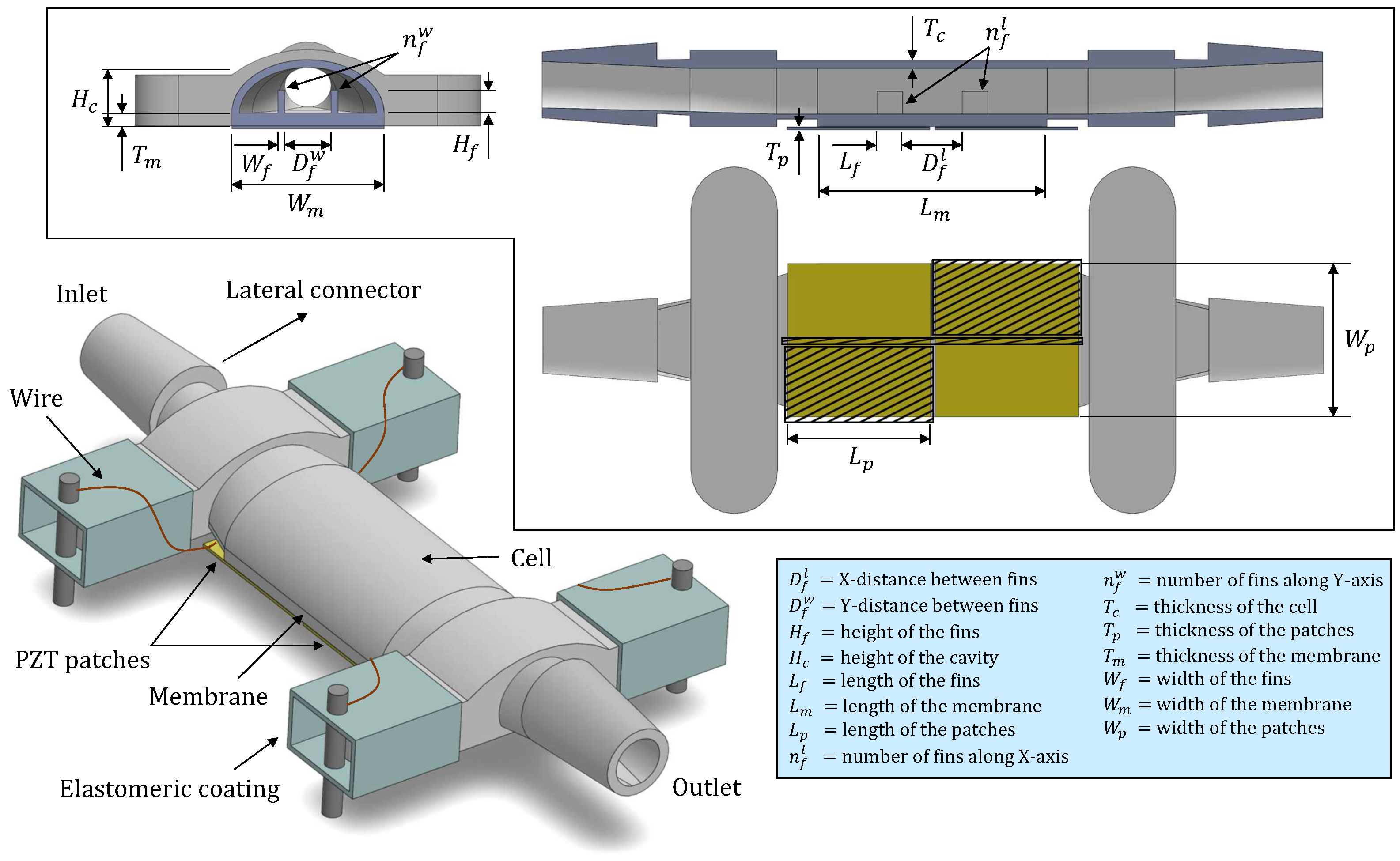
Figure 2.
Simulated membranes with piezoelectric patches for actuation (depicted in red), and signal detection (shown in blue).
Figure 2.
Simulated membranes with piezoelectric patches for actuation (depicted in red), and signal detection (shown in blue).
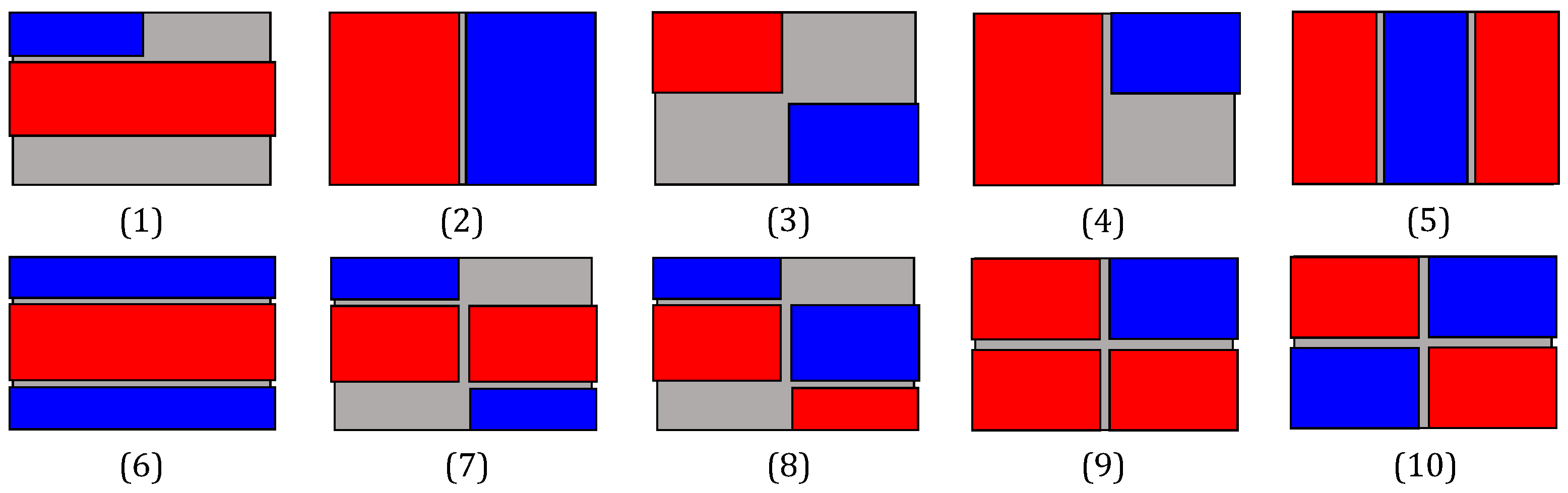
Figure 3.
In-plane stress distribution, averaged across all modal forms between 1 kHz and 1 MHz. Positive values are represented in red, negative values in blue, and low-stress regions in white. Sensor patches are delineated in black.
Figure 3.
In-plane stress distribution, averaged across all modal forms between 1 kHz and 1 MHz. Positive values are represented in red, negative values in blue, and low-stress regions in white. Sensor patches are delineated in black.
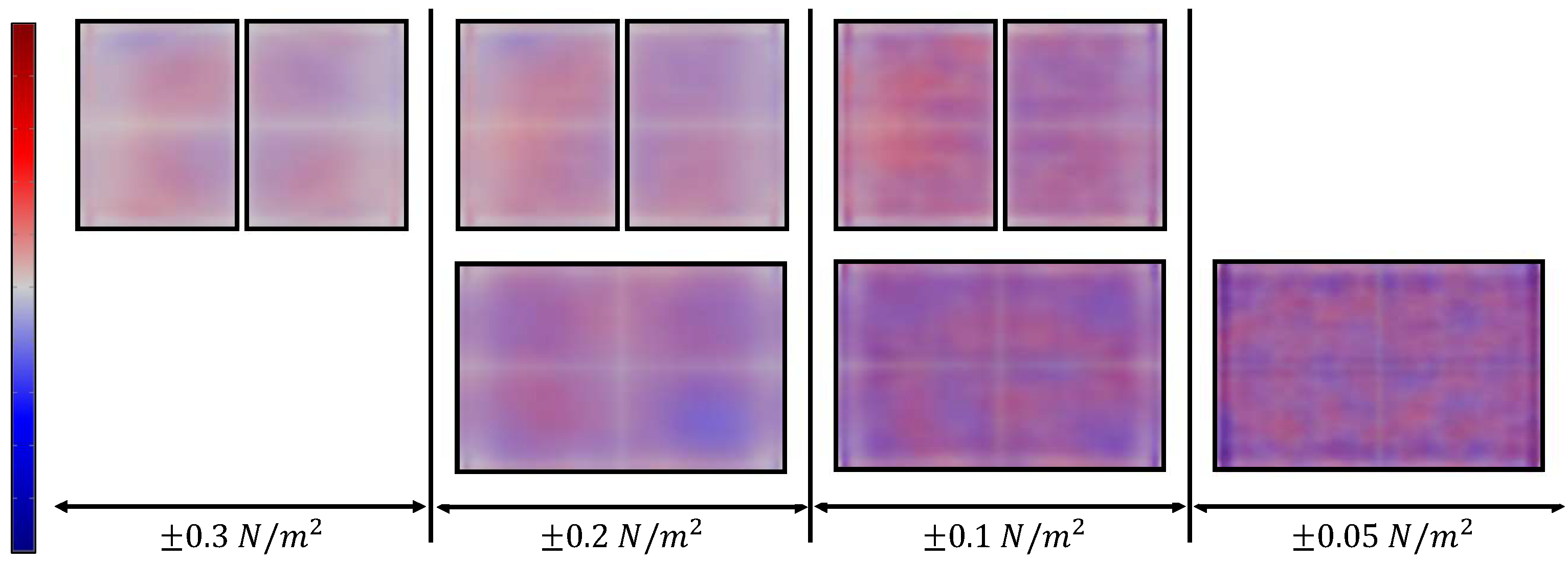
Figure 4.
Architecture of our sensor system. A schematic illustration of the sensor, signal conditioning circuits, and microcontroller is provided.
Figure 4.
Architecture of our sensor system. A schematic illustration of the sensor, signal conditioning circuits, and microcontroller is provided.
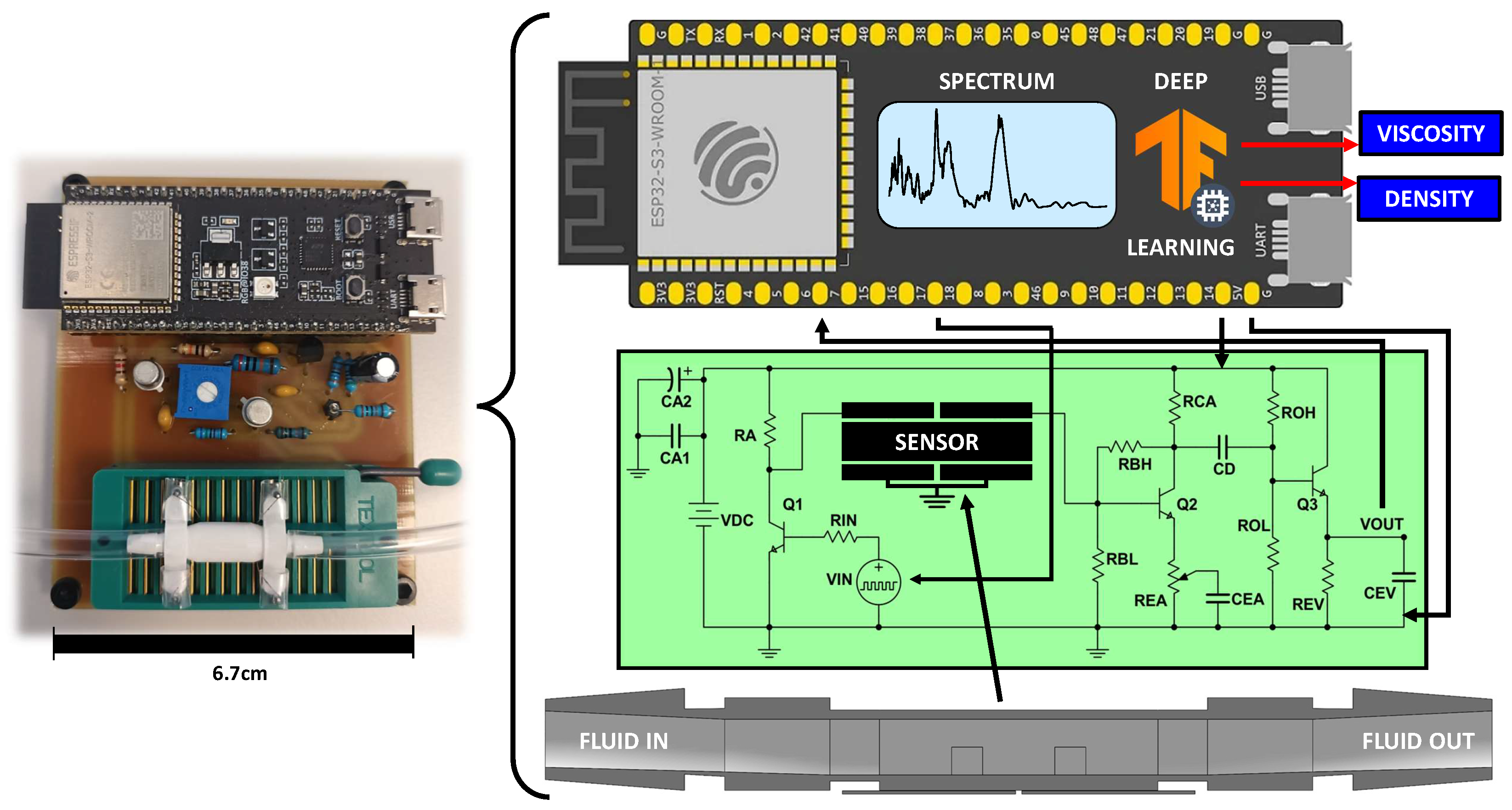
Figure 5.
Comparison of the performance of two geometries: the left graph depicts a cell with poorer m and performance in the sensitivity-reproducibility/recovery game, while the right figure shows a cell with improved performance across this metric.
Figure 5.
Comparison of the performance of two geometries: the left graph depicts a cell with poorer m and performance in the sensitivity-reproducibility/recovery game, while the right figure shows a cell with improved performance across this metric.
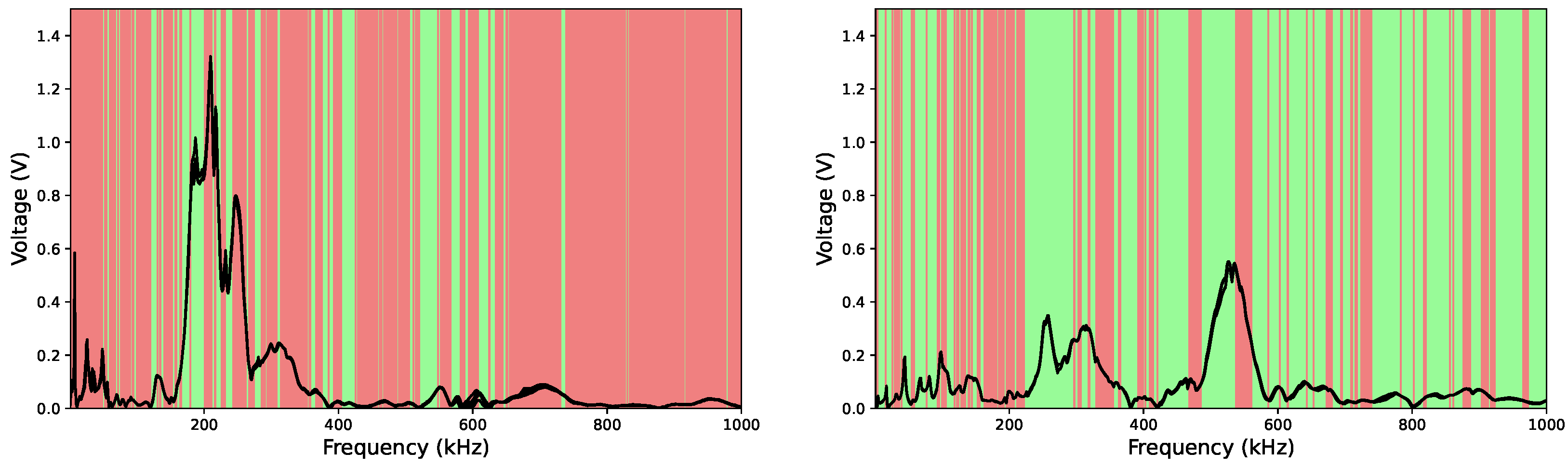
Figure 6.
Sensor obtained through the structural refinement process. Three views are presented: an overview (left), a plan view (right), and an interior view of the cell showing the arrangement of fins attached to the membrane (top center).
Figure 6.
Sensor obtained through the structural refinement process. Three views are presented: an overview (left), a plan view (right), and an interior view of the cell showing the arrangement of fins attached to the membrane (top center).
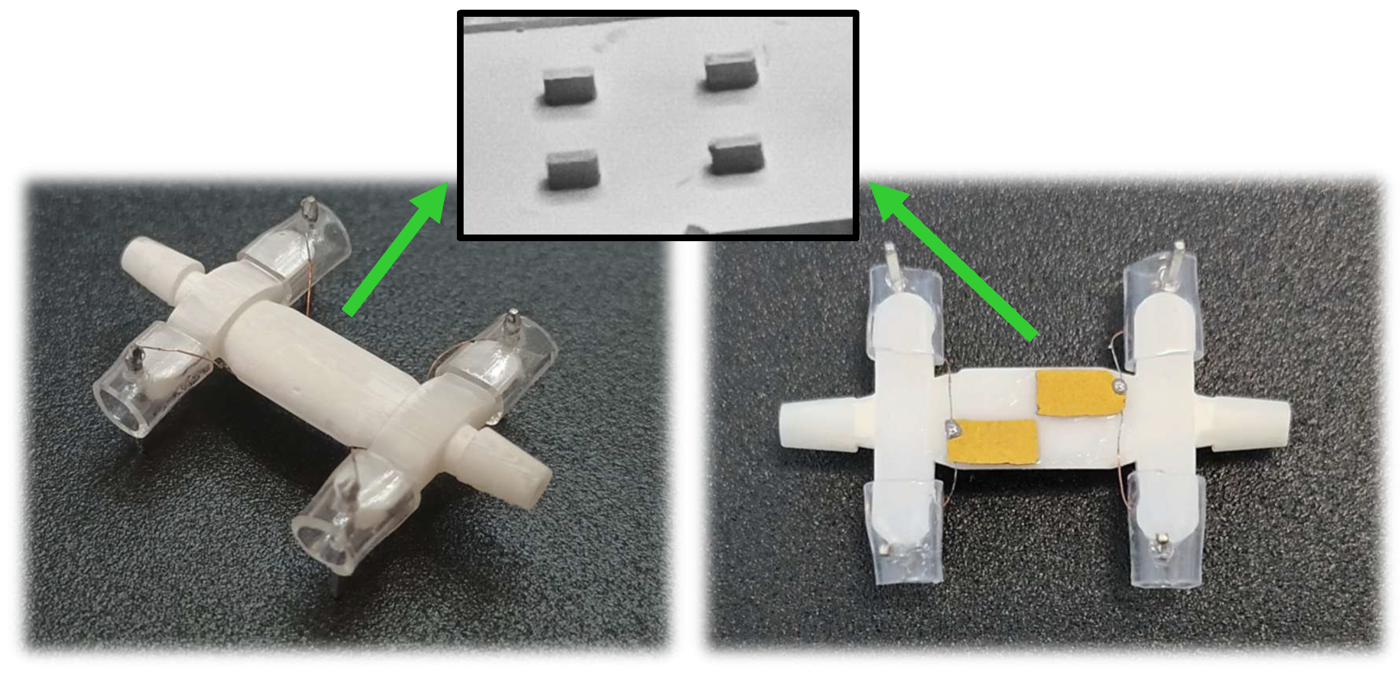
Figure 7.
(a) Spectra collected by our liquid monitoring system for each solution in Table 2. (b) Optimized neural network architecture for viscosity and density estimation based on the N-labeled spectra in (a).
Figure 7.
(a) Spectra collected by our liquid monitoring system for each solution in Table 2. (b) Optimized neural network architecture for viscosity and density estimation based on the N-labeled spectra in (a).
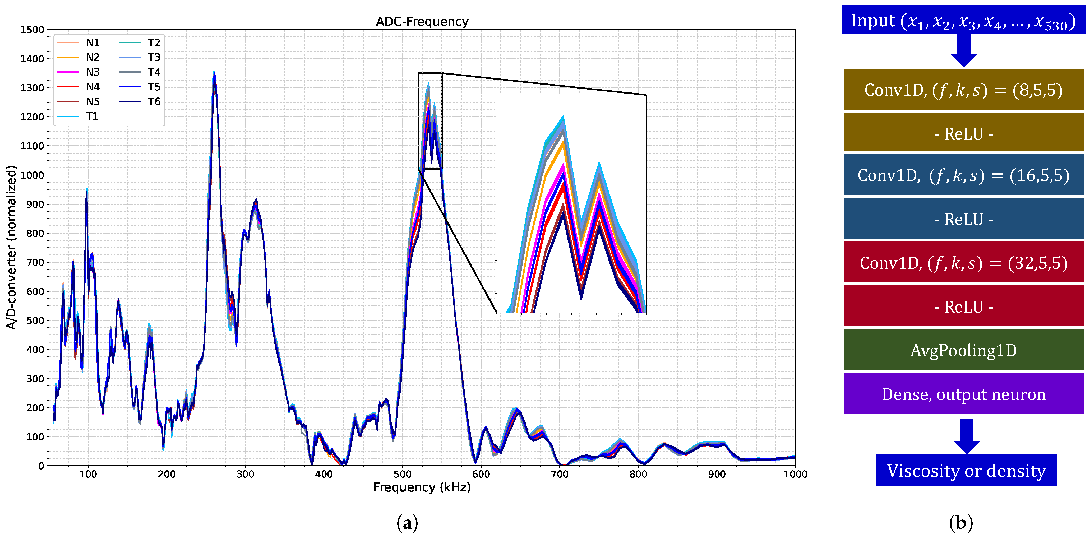
Figure 8.
(a) Viscosity model predictions for the training set (red) and test set (blue), compared with measurements from the commercial viscometer (green). (b) Density model predictions for the training set (green) and test set (orange), compared with the reference measurements (blue). (c) Viscosity predictions for four solutions at day 0 (red) and over four subsequent days after applying the data correction procedure (blue), compared with the reference values (green). (d) Density predictions for four solutions at day 0 (green) and over four subsequent days after applying the data correction procedure (orange), compared with the reference values (blue).
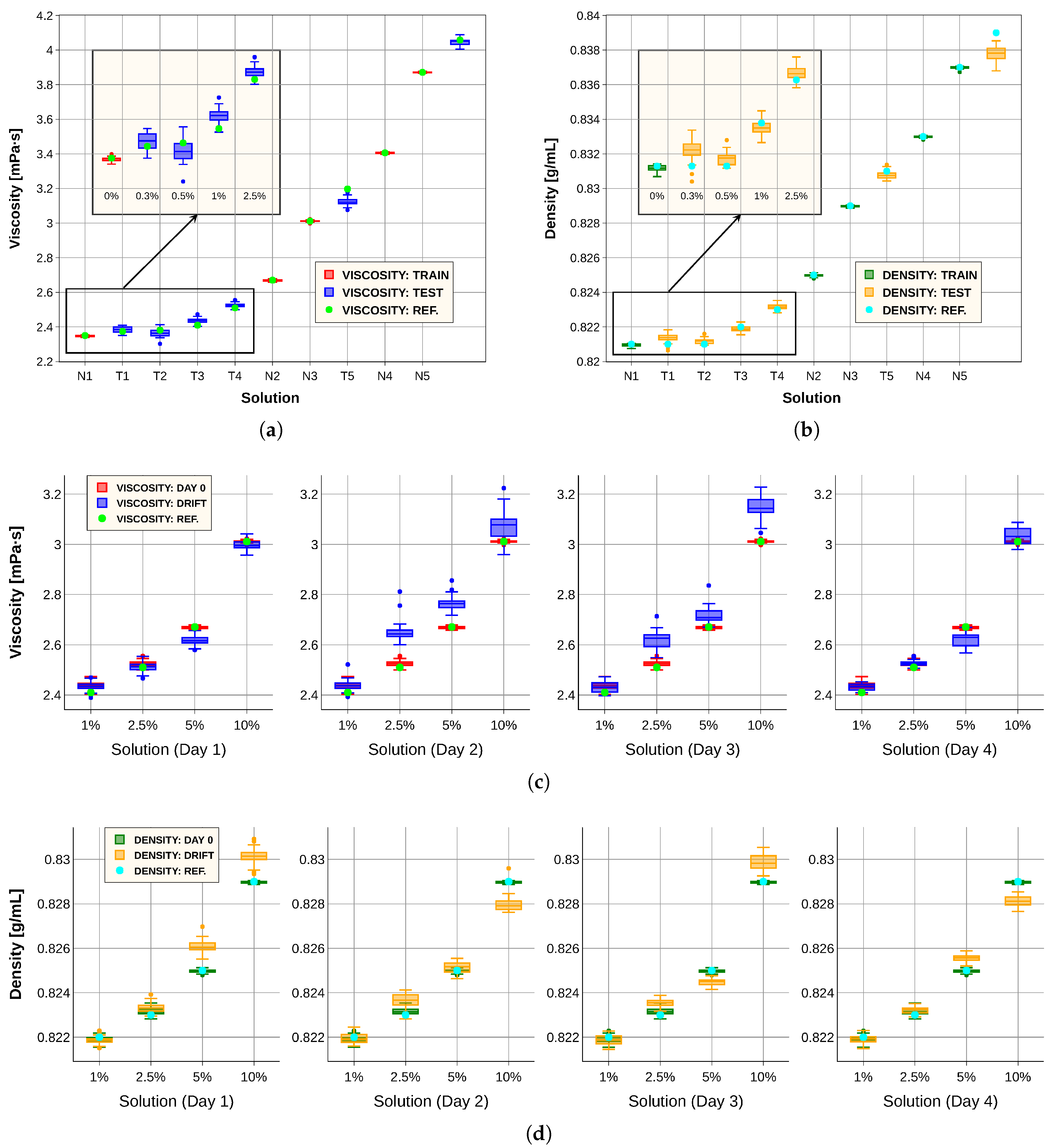
Figure 9.
Results obtained with models trained with 103-point spectra. (a) Viscosity model predictions for the training set (red) and test set (blue), compared with measurements from the commercial viscometer (green). (b) Density model predictions for the training set (green) and test set (orange), compared with the reference measurements (blue). (c) Viscosity predictions for four solutions at day 0 (red) and over four subsequent days after applying the data correction procedure (blue), compared with the reference values (green). (d) Density predictions for four solutions at day 0 (green) and over four subsequent days after applying the data correction procedure (orange), compared with the reference values (blue).
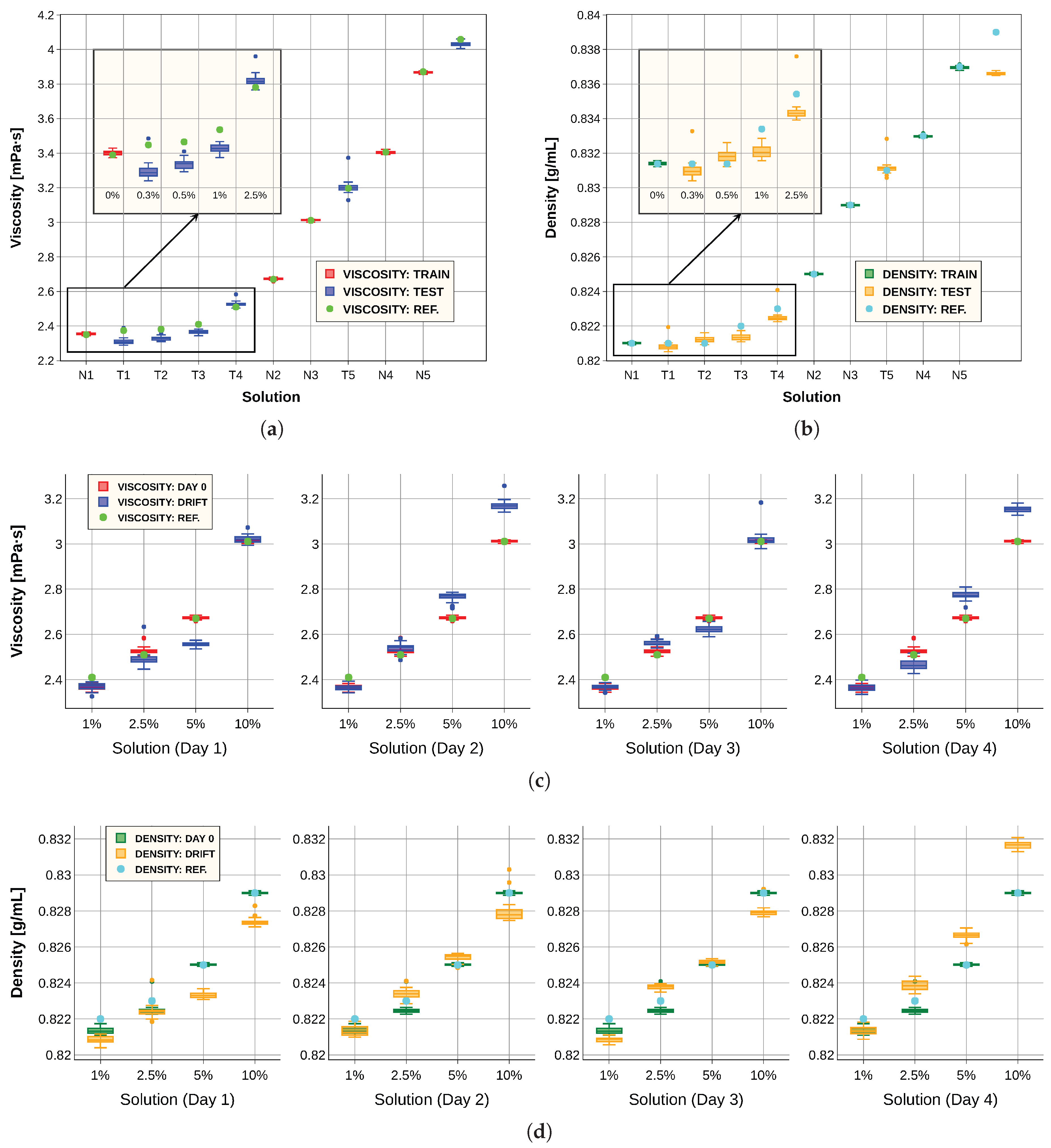

Table 1.
Description and dimensional specification of the geometric parameters investigated during the sensor optimization process.
Table 1.
Description and dimensional specification of the geometric parameters investigated during the sensor optimization process.
| Label | Description | Minimum (mm) | Maximum (mm) |
|---|---|---|---|
| X-distance between fins | 1 | 4 | |
| Y-distance between fins | 0.8 | 1.82 | |
| height of the fins | 0.9 | 1.8 | |
| height of the cavity | 1.8 | 1.8 | |
| length of the fins | 0.5 | 2 | |
| length of the membrane | 8 | 17 | |
| length of the patches | |||
| number of fins along X-axis | 0 | 4 | |
| number of fins along Y-axis | 0 | 3 | |
| thickness of the cell | 0.2 | 0.3 | |
| thickness of the patches | 0.11 | 0.11 | |
| thickness of the membrane | 0.2 | 0.5 | |
| width of the fins | 0.14 | 0.6 | |
| width of the membrane | 4 | 14 | |
| width of the patches |
Table 2.
Composition of the biofuels employed with the corresponding viscosity and density values.
| Label | Description | (mPa·s) | (g/mL) |
|---|---|---|---|
| 100% Diesel - 0% Sunflower oil | 2.350 | 0.821 | |
| 95% Diesel - 5% Sunflower oil | 2.670 | 0.825 | |
| 90% Diesel - 10% Sunflower oil | 3.011 | 0.829 | |
| 85% Diesel - 15% Sunflower oil | 3.406 | 0.833 | |
| 80% Diesel - 20% Sunflower oil | 3.871 | 0.837 | |
| 99.7% Diesel - 0.3% Sunflower oil | 2.374 | 0.821 | |
| 99.5% Diesel - 0.5% Sunflower oil | 2.381 | 0.821 | |
| 99% Diesel - 1% Sunflower oil | 2.410 | 0.822 | |
| 97.5% Diesel - 2.5% Sunflower oil | 2.510 | 0.823 | |
| 87.5% Diesel - 12.5% Sunflower oil | 3.197 | 0.831 | |
| 78% Diesel - 22% Sunflower oil | 4.058 | 0.839 |
Table 3.
General structure of the tested convolutional neural networks.
| Input: spectrum of 530 components | |
| Convolutional blocks ∈ [3,4] | Number of filters ∈ [8,64] |
| Kernel size ∈ [3,13] | |
| Stride ∈ [2,7] | |
| ReLU activation function | |
| MaxPooling 1D, size = 1/2 | |
| Average pooling 1D | |
| Fully connected 1. Output: Viscosity or Density | |
Table 4.
Dimensions of the best sensor found in experiments.
| Label | Description | Value (mm) |
|---|---|---|
| X-distance between fins | 2.33 | |
| Y-distance between fins | 1.82 | |
| height of the fins | 0.9 | |
| height of the cavity | 1.8 | |
| length of the fins | 1 | |
| length of the membrane | 9 | |
| length of the patches | ||
| number of fins along X-axis | 2 | |
| number of fins along Y-axis | 2 | |
| thickness of the cell | 0.3 | |
| thickness of the patches | 0.11 | |
| thickness of the membrane | 0.5 | |
| width of the fins | 0.27 | |
| width of the membrane | 6 | |
| width of the patches |
Table 5.
Error values obtained from viscosity predictions obtained with the proposed system.
| Dataset | Calibration | Resolution | ||
|---|---|---|---|---|
| Train (N) | 0.2 | 0.12 | ||
| Test (T) | 1.64 | 0.99 | ||
Table 6.
Error values obtained from density predictions obtained with the proposed system.
| Dataset | Calibration | Resolution | ||
|---|---|---|---|---|
| Train (N) | 0.29 | |||
| Test (T) | 2.24 | |||
Table 7.
Comparison of viscosity prediction errors between day 0 and subsequent days.
| Dataset | Calibration | Resolution | ||
|---|---|---|---|---|
| Data 0 | 2.12 | 0.51 | ||
| Data drift | 9.08 | 2.04 | ||
Table 8.
Comparison of density prediction errors between day 0 and subsequent days.
| Dataset | Calibration | Resolution | ||
|---|---|---|---|---|
| Data 0 | 1.6 | |||
| Data drift | 7.87 | |||
Table 9.
Errors in viscosity estimation for the test dataset using models trained with spectra of varying dimensionality.
Table 9.
Errors in viscosity estimation for the test dataset using models trained with spectra of varying dimensionality.
| Points (Dataset) | Calibration | Resolution | ||
|---|---|---|---|---|
| 530 (T) | 1.64 | 0.99 | ||
| 244 (T) | 1.35 | 0.84 | ||
| 103 (T) | 2.18 | 1.44 | ||
Table 10.
Errors in density estimation for the test dataset using models trained with spectra of varying dimensionality.
Table 10.
Errors in density estimation for the test dataset using models trained with spectra of varying dimensionality.
| Points (Dataset) | Calibration | Resolution | ||
|---|---|---|---|---|
| 530 (T) | 2.24 | |||
| 244 (T) | 3.14 | |||
| 103 (T) | 3.95 | |||
Table 11.
Errors in viscosity estimation from the drift experiment, using the spectral correction method and models trained with spectra of different numbers of points.
Table 11.
Errors in viscosity estimation from the drift experiment, using the spectral correction method and models trained with spectra of different numbers of points.
| Points (Dataset) | Calibration | Resolution | ||
|---|---|---|---|---|
| 530 (drift) | 10.12 | 2.28 | ||
| 244 (drift) | 8.67 | 1.93 | ||
| 103 (drift) | 10.52 | 2.35 | ||
Table 12.
Errors in density estimation from the drift experiment, using the spectral correction method and models trained with spectra of different numbers of points.
Table 12.
Errors in density estimation from the drift experiment, using the spectral correction method and models trained with spectra of different numbers of points.
| Points (Dataset) | Calibration | Resolution | ||
|---|---|---|---|---|
| 530 (drift) | 8.027 | |||
| 244 (drift) | 12.48 | 0.11 | ||
| 103 (drift) | 15.03 | 0.13 | ||
Table 13.
Comparison of viscosity results obtained in this work with those reported in the literature [25,26,31,32,33,35,36,43].
| Error | Our work | [43] | Outperformed by (excluding [43]) |
|---|---|---|---|
| - | |||
| 1.64 | 1.41 | - | |
| 0.99 | 0.8 | 0.792 - [33] | |
| [2.7-7.8] - [25,26,32] |
Short Biography of Authors
Víctor Corsino is a PhD student in Science and Technology Applied to Industrial Engineering, Universidad de Castilla-La Mancha (UCLM), Spain. He has a degree in Electronic Engineering from this university, with a mention in advanced electronic technologies, and a Master’s degree in Artificial Intelligence from Universidad Politécnica de Madrid (UPM). Since 2023 is part of Microsystems, Actuators and Sensors Group. His current research interests include pattern recognition, machine learning and microsensors with liquid media applications.
Víctor Ruiz-Díez is an Assistant Professor, holding a degree in Industrial Engineering, with a mention in Electronics and Automation, from the Universidad de Castilla-La Mancha, Spain, and a Master’s degree in Physics and Mathematics from the same university and Universidad de Granada. He earned his Ph.D. in Applied Sciences and Technologies for Industrial Engineering from the Universidad de Castilla-La Mancha, where he specialized in high-performance MEMS resonators for liquid media applications. His work has garnered recognition with numerous publications and contributions at international conferences. Currently, he leads research on MEMS applications in terrestrial and liquid locomotion using advanced 3D printing techniques.
Andrei Braic is a Ph.D. student in Electronic Engineering at the Universidad de Castilla-La Mancha (UCLM), Spain. He holds a degree in Electronic Engineering from UCLM and a Master’s in Systems and Control Engineering from UNED. He’s part of the Microsystems, Actuators and Sensors (MAS) Group, and his research focuses on piezoelectric actuation combined with 3D-printing techniques for sensors and actuators.
José Luis Sánchez-Rojas received the M.S., and Ph.D. degrees in telecommunication engineering from the Universidad Politécnica de Madrid, Spain. In 1997, he was an Invited Postdoctoral Scientist with Cornell University, Ithaca, NY, and Colorado University, Boulder. He is currently a Full Professor with the Universidad de Castilla-La Mancha, and head of the Microsystems, Actuators and Sensors Lab. His research interests cover smart microdevices, miniaturization, microrobot locomotion, design and applications of MEMS/NEMS, sensors and actuators.
Disclaimer/Publisher’s Note: The statements, opinions and data contained in all publications are solely those of the individual author(s) and contributor(s) and not of MDPI and/or the editor(s). MDPI and/or the editor(s) disclaim responsibility for any injury to people or property resulting from any ideas, methods, instructions or products referred to in the content. |
© 2025 by the authors. Licensee MDPI, Basel, Switzerland. This article is an open access article distributed under the terms and conditions of the Creative Commons Attribution (CC BY) license (http://creativecommons.org/licenses/by/4.0/).
Copyright: This open access article is published under a Creative Commons CC BY 4.0 license, which permit the free download, distribution, and reuse, provided that the author and preprint are cited in any reuse.


