Submitted:
25 November 2025
Posted:
26 November 2025
You are already at the latest version
Abstract
Formal verification has achieved remarkable outcomes in both theory advancement and engineering practice, with the formalization of mathematical theories serving as its foundational cornerstone—making this process particularly critical. Axiomatic set theory underpins modern mathematics, providing the rigorous basis for constructing almost all theories. Landau's Foundations of Analysis starts with pure logical axioms from set theory, does not rely on geometric intuition, strictly constructs number systems, and is a benchmark for axiomatic analysis in modern mathematics. In this paper, we first develop a machine proof system for axiomatic set theory rooted in the Morse-Kelley (MK) system. This system encompasses proof automation, scale simplification, and specialized handling of the Classification Axiom for ordered pairs. We then prove the Transfinite Recursion Theorem, leveraging it to further prove the Recursion Theorem for natural numbers the key result for defining natural number operations.
Finally, we detail the implementation of a machine proof system for analysis, which adopts MK as its description language and adheres to Landau’s Foundations of Analysis. This formalization can be relatively seamlessly ported to type theory-based real analysis. Implemented using the Rocq proof assistant, the formalization has undergone verification to ensure completeness and consistency. This work holds broader applicability, and it can be extended to the formalization of point-set topology and abstract algebra, while also serving as a valuable resource for teaching axiomatic set theory and mathematical analysis.
Keywords:
formal verification
; foundations of analysis
; axiomatic set theory
; Rocq
; Recursion Theorem
MSC: 68V20
1. Introduction
Formal verification for mathematics aims to formalize mathematical theories through computers verification. Gödel once stated, "The development of mathematics towards greater exactness has, as is well-known, lead to formalization of large areas of it such that you can carry out proofs by following a few mechanical rules. " In recent decades, formalization technology has become an important tool in mathematical theory [36,37] and program verification[1,39].
Formal tools have rapidly developed alongside innovations in underlying theories, resulting in stronger expressive power, closer alignment with mathematical notation, better interactivity, and higher levels of automation[24,26,38]. The pioneering computer proof tool Automath was developed by de Bruijn in the late 1960s, with the aim of expressing mathematical proofs through a computer language[2]. As the first successful application of the Curry-Howard isomorphism, many of its design principles were not fully appreciated at the time. However, as type theory and computer tools advanced, it provided a strong foundation for the development of modern higher-order logic provers[29,30].
Rocq(formerly known as Coq)[3,7,8], an interactive proof assistant based on constructive calculus theory[10,11,34], is one of the most popular provers founded on the type theory. Gonthier and his team completed the formal proof of the "Four Color Theorem"[18] and the "Odd Order Theorem" [16], causing a great sensation in the mathematical and computer fields. Boldo had formalized the Lebesgue integration of nonnegative functions, whcih is of great significance for toward the formalization of spaces such as Banach spaces. Cao introduced Rocq into teaching to help students understand the contents in a deep and comprehensive way, without missing any key concepts. Shao Zhong, Gu Ronghui and other researchers successfully developed the world’s first fully formally verified operating system kernel with no vulnerabilities: CertiKOS[21]. Cohen and Johnson-Freyd developed a natural deduction proof system for Why3. It can be seen from these abundant achievements that formal verification has achieved fruitful results both in theoretical development and engineering applications[12,25,28], and the formalization of mathematical theories as foundation, is particularly important.
Set theory plays an extremely important role in mathematics because its concepts are involved in nearly every branch of mathematics[23]. At the same time, set theory has significant applications in computer science, artificial intelligence, logic and other fields. The third mathematical crisis prompted mathematicians to begin the axiomatization of set theory, which involved limiting the definitions in naive set theory through axioms[4]. In 1908, the German mathematician Zermelo first published an axiomatic system for set theory, which was later improved and modified by mathematicians Fraenkel and Skolem, forming the well-known Zermelo-Fraenkel set theory axiom system(ZF). In 1920, Hungarian-American mathematician von Neumann proposed another axiomatic system[27], which was modified by Bernays starting in 1937 and further simplified by Gödel in 1940, resulting in the famous von Neumann-Bernays-Gödel set theory axiom system(NBG). Subsequently, other axiomatic set theory systems such as Morse-Kelley(MK) set theory[31,35] and Tarski-Grothendieck set theory were developed. Axiomatic set theory has provided a convenient and practical language and tool for mathematical research, thereby making set theory the foundation of modern mathematical theory once again.
The axiomatic system for natural number took shape based on basic properties summarized by Dedekind, with its landmark being Peano’s 1889 work Arithmetices Principia, Nova Methodo Exposita (The Principles of Arithmetic, Presented by a New Method). After numerous failures and setbacks, efforts to find a foundation for analytical mathematics[42] gradually gained clarity — the process known as the "arithmetization of analysis" in the 19th century, which generally unfolded in three stages[9,19]: (1) establishment of the limit theory: marked primarily by the work of Cauchy and Weierstrass. (2) establishment of the real number theory: defined mainly by the real number construction theories developed by Dedekind, Cantor, and Weierstrass, among others. (3) completion of the arithmetization process: symbolized by the natural number theories proposed by Dedekind and Peano. It is evident that the arithmetization of analysis is closely linked to the resolution of the three famous crises in the history of mathematics.
In this work, we first present the machine proof system of Morse-Kelley axiomatic set theory which is concise yet comprehensive for analysis. This part of the content includes not only our formalization but also the optimization and vulnerability patching compared to previous work[40]. Next, we prove Transfinite Recursion Theorem which is one of most important conclusions in MK. Moreover, through this theorem we prove Recursion Theorem for natural numbers, which is a crucial conclusion for defining natural number operations. At last, we present the implementation details of machine proof system for analysis including natural numbers, fractions, cuts, real numbers, complex numbers which follows Landau’s Foundations of Analysis and uses the MK as the foundational description language. Every proof is verified by Rocq to show rigor and correctness and we make up for missing proof details to make it more complete.
The paper is organized in the following way. Section 2 is dedicated to related work. Section 3 states contents of the MK including axioms, notations, definitions and properties for understanding this work. Section 4 introduces the proof details of Transfinite Recursion Theorem and Recursion Theorem for natural numbers. Section 5 presents the formalization of analysis from natural numbers to complex numbers. Finally, we draw our conclusions and discuss some potential further work in Section 6.
2. Related Work
In the formalizations of set theory, Simpson developed the axiomatization of ZFC and formalized common set-theoretic concepts. Kirst and Smolka completed the formal construction of second-order ZF set theory[32]. Paulson constructed the ZFC set theory based on the formalization tool Isabelle/ZF. On the other hand, there already exists some formalizations of Landau’s “Foundations of Analysis”[33]. de Bruijn designed earliest proof checker Automath, and his student van Benthem Jutting has completed the formalization of Landau’s “Foundations of Analysis” in AUT-QE[2]. Moreover, Brown has given a particular faithful reproduction of a signature corresponding to the Automath version of Landau’s book[6]. Guidi encoded this book into the formal language ’’, furthermore, presents an implemented procedure producing a representation of the “Foundations of Analysis” in Rocq[22]. In addition to the above work, Grimm has defined real numbers from set theory, and he aims to formalize the fundamental notations of mathematics referring to “Elements of Mathematics” of Bourbaki[20]. In Rocq’s standard library, there is already a set of real number theories based on a dozen axioms[17]. The excellent real analysis library—Coquelicot[5]—is developed by Boldo et al. as an extension of the library.
In our previous work, we had completed the machine proof system of axiomatic set theory and analysis[41], which are significantly different from the work in this paper. Regarding axiomatic set theory, we have addressed the existing defects about classifier, added a series of automated strategies and conclusions with independent significance to facilitate expansion, and furthermore, we have proven the key proposition Recursion Theorem for defining natural number operations. The formalization of Recursion Theorem based on the Transfinite Recursion Theorem is the first of its kind to our knowledge. In terms of analysis, we completed the formalization of the equivalence among completeness theorems of real number[14], the properties of continuous functions on closed intervals[13] and the rigor of calculus without limit theory[15], however, all this work is based on type theory, which is fundamentally different from our work at the underlying level.
3. Morse-Kelley Axiomatic Set Theory
Considering consistency the description of the axioms, definitions and theorems involved in the formalization corresponds to one in Kelley’s General Topology. Meanwhile, we just extract the content required by the formalization for the sake of code simplicity and readability. The MK theory itself is a metalanguage, and few additional elements need to be introduced such as logical constants and quantifications, that and equality in MK are consistent with the conventional meaning. Moreover, this theory is built on classical logic, hence the law of excluded middle need be introduced. Then the MK system can be start builded with these foundations.
We first declare a "class," which is the type of all objects (whether they are sets or not). The formal description in Rocq is as follows:
- Parameter Class :Type.
Additionally, two mathematical constants and the concept of set need to be introduced. The first constant of these is “∈” and “” is called “e is a element of C ” or “e belongs to C”. The second constant one of these is “” which denotes a classifier, that is, the class composed of all classes that satisfy a certain property. Next, if “s” is a set, it indicates that “s” belongs to a certain class. Their formal descriptions in Rocq is as follows:
- Parameter In : Class -> Class -> Prop.
- Notation "x ∈ y" := (In x y) (at level 10).
- Parameter Classifier : (Class -> Prop) -> Class.
- Notation "\{ P \}" := (Classifier P) (at level 0).
- Definition Ensemble (s :Class) = ∃ C, s ∈ C.
There are a total of 8 axioms and 1 axiomatic-scheme about the extensionality of equality, classifier, the judgment of whether a special class is a set, the existence of countably infinite sets and the axiom of choice. The descriptions of these propositions and their formalizations in Rocq are as follows:
Axiom of extent:
Classification axiom-scheme: is a set and
Axiom of subsets: x is a s set is a s set,
Axiom of union: Both are sets is a set.
Axiom of substitution: The domain of function f is a set → Ran(f) is a set.
Axiom of amalgamation: x is a set is a set.
Axiom of regularity:
Axiom of infinity: is a set, and whenever .
Axiom of choice: There is a choice function c whose domain is .
- Axiom AxiomI : ∀ x y, x = y <-> (∀ z, z ∈ x <-> z ∈ y).
- Axiom AxiomII : ∀ b P, b ∈ \{ P \} <-> Ensemble b /\ (P b).
- Axiom AxiomIII : ∀ {x}, Ensemble x -> ∃ y, Ensemble y /\ (∀ z, z ⊂ x -> z ∈ y).
- Axiom AxiomIV : ∀ {x y}, Ensemble x -> Ensemble y -> Ensemble (x∪y).
- Axiom AxiomV : ∀ {f}, Function f -> Ensemble dom(f) -> Ensemble ran(f).
- Axiom AxiomVI : ∀ x, Ensemble x -> Ensemble (∪ x).
- Axiom AxiomVII : ∀ x, x ≠ Ø -> ∃ y, y ∈ x /\ x ∩ y = Ø.
- Axiom AxiomVIII : ∃ y, Ensemble y /\ Ø ∈ y /\ (∀ x, x ∈ y -> x∪[x] ∈ y).
- Axiom AxiomIX : ∃ c, ChoiceFunction c /\ dom(c) = μ ̃ [Ø].
Except for the details of classification axiom-scheme, all the axioms above is similar to other axiomatic set theory systems, but this one is the key that cannot be lacking. We can resolve Russell Paradox, that is, proper class is not a set by the classification axiom-scheme. Firstly, we named Russell’s class as R whose definition is as follows:
Supposing the R is a set. If , we can get R is a set and by classification axiom-scheme. If , we can get by classification axiom-scheme and R is a set. Both situations above are self-contradictory, therefore Russell’s class is not a set. In addition, it can be concluded that is not a set by this conclusion.
In our early formalization for MK, we had completed almost the all content, however, there are some aspects need to be improved. Therefore, we upgrade the original system, and solve the remaining problems in this work.
3.1. Optimization and Automation
In Rocq, the integration of proof tactics can be achieved through "Ltac", which is highly necessary in the machine proof system for axiomatic set theory. This is because it can help reduce the proofs related to sets in subgoals and provide concise instructions to replace lengthy commands, thereby improving efficiency. The following briefly shows the handling of instructions, quantifiers, sets, and other aspects in the code.
- (* Simplification for existential quantifier in the hypothesis *)
- Ltac deHex1 :=
- match goal with
- H: ∃ x, ?P
- |- _ => destruct H as []
- end.
- Ltac rdeHex := repeat deHex1; deand.
- (* Simplification for empty-class *)
- Ltac eqext := apply AxiomI; split; intros.
- (* Simplification for classification axiom-scheme *)
- Ltac appA2G := apply AxiomII; split; eauto.
- Ltac appA2H H := apply AxiomII in H as [].
- Ltac PP H a b := apply AxiomII in H as [? [a [b []]]]; subst.
- Ltac appoA2G := apply AxiomII’; split; eauto.
- Ltac appoA2H H := apply AxiomII’ in H as [].
- (* Simplification for intersection and union *)
- Ltac deHun :=
- match goal with
- | H: ?c ∈ ?a ∪ ?b
- |- _ => apply MKT4 in H as [] ; deHun
- | _ => idtac
- end.
- Ltac deGun :=
- match goal with
- | |- ?c ∈ ?a∪?b => apply MKT4 ; deGun
- | _ => idtac
- end.
- Ltac deHin :=
- match goal with
- | H: ?c ∈ ?a ∩ ?b
- |- _ => apply MKT4’ in H as []; deHin
- | _ => idtac
- end.
- Ltac deGin :=
- match goal with
- | |- ?c ∈ ?a ∩ ?b => apply MKT4’; split; deGin
- | _ => idtac
- end.
- (* Simplification for empty-class *)
- Ltac emf :=
- match goal with
- H: ?a ∈ Ø
- |- _ => destruct (MKT16 H)
- end.
- Ltac eqE := eqext; try emf; auto.
- Ltac feine z := destruct (@ MKT16 z).
- Ltac NEele H := apply NEexE in H as [].
- (* Simplification for ordered pair *)
- Ltac ope1 :=
- match goal with
- H: Ensemble ([?x,?y])
- |- Ensemble ?x => eapply MKT49c1; eauto
- end.
- Ltac ope2 :=
- match goal with
- H: Ensemble ([?x,?y])
- |- Ensemble ?y => eapply MKT49c2; eauto
- end.
- Ltac ope3 :=
- match goal with
- H: [?x,?y] ∈ ?z
- |- Ensemble ?x => eapply MKT49c1; eauto
- end.
- Ltac ope4 :=
- match goal with
- H: [?x,?y] ∈ ?z
- |- Ensemble ?y => eapply MKT49c2; eauto
- end.
- Ltac ope := try ope1; try ope2; try ope3; try ope4.
- Ltac xo :=
- match goal with
- |- Ensemble ([?a, ?b]) => try apply MKT49a
- end.
- Ltac rxo := eauto; repeat xo; eauto.
- (* Simplification for mathematical induction *)
- Ltac MI x := apply Mathematical_Induction with (n:=x); auto; intros.
Furthermore, enabling researchers to focus their proof ideas on the core part, we have extracted many propositions with general significance and added numerous inferences with wide applications. There are 40 lemmas,16 corollaries, 50 facts, and 30 integrated proof strategies carrying out simplification work. As a result, we reduce the overall code size to half of its original size.
3.2. Classification Axiom-Scheme for Ordered Pair
When classification axiom-scheme was first proposed in MK, it took a general form, so it should naturally be applicable to various situations. However, when the elements in a class are ordered pairs (i.e., there exist two variables), they must be handled reasonably in formalization; otherwise, the kernel verification cannot be passed. In the early work, we newly defined a classifier for ordered pairs and added 2 axioms following the example of classification axiom-scheme. The specific details of the formalization are as follows.
Origin code:
- Parameter Classifier_P : (Class -> Class -> Prop) -> Class.
- Notation "\{\ P \}\" := (Classifier_P P) (at level 0).
- Axiom AxiomII_P : ∀ a b P, [a, b] ∈ \{\ P \}\ <-> Ensemble [a, b] /\ (P a b).
- Axiom Property_P : ∀ z P, z ∈ \{\ P \}\ -> (∃ a b, z = [a, b]) /\ z ∈ \{\ P \}\.
It should be noted here that the statements of "Parameter" and "Axiom" are directly acknowledged without the need for proof, therefore it is necessary to propose with caution. In this work, we prove the additional three admitted propositions about the ordered pair and provide a better handling method to address the weakness. The formalization of the classification axiom-scheme for ordered pair is shown in the following code.
Updated code:
- Notation "\{\ P \}\" := \{ λ z, ∃ x y, z = [x, y] /\ P x y \}(at level 0).
- Fact AxiomII’ : ∀ a b P, [a, b] ∈ \{\ P \}\ <-> Ensemble [a, b] /\ (P a b).
The statements of “Fact” need to be proven, which means the description is rigorous. Hence we can get the additional three axioms previously added is rational but unnecessary. These propositions verified by Rocq ensure the non-contradiction of the entire system.
3.3. Essential Content for Analysis
The formalization of analysis does not need to introduce the content related to the Axiom of Choice and subsequent content concerning cardinal numbers in MK. Meanwhile, the machine proof system of axiomatic set theory can be designed to be self enclosed and does not require the introduction of additional content, hence we only retained previous content of Axiom of Choice but not including Axiom of Choice. The following table lists the essential definitions and their corresponding symbols in MK to formalize FA.

Table 1.
Definitions and meanings in MK.
| Rocq Symbol | Meaning |
|---|---|
| a is an element of the class A | |
| Ensemble A | A is a set |
| or | |
| and | |
| and | |
| ∅ | empty class |
| proper class | |
| A is a subclass of B | |
| ordered pair | |
| Function f | f is a function |
| dom(f) | domain of f |
| ran(f) | range of f |
| value of f at a | |
| Oridinal r | r is an ordinal |
| R | class of all ordinal numbers |
| Oridinal_Number r | r is an ordinal number |
| restriction of f on x | |
| OnTo F A B | function F is from A to B |
| PlusOne n | successor of n |
| W | class of all integer numbers |
For sake of understanding, the specific content of the definitions and their respective formalizations are presented as follows.
• The empty class ∅ is a class without any elements.
- Definition Ø := \{λ x, x ≠ x \}.
• Their proper class is a class composed of all sets.
- Definition μ := \{λ x, x = x \}.
•f is a function that means it is composed of ordered pairs, and if the first coordinate of any element in f is fixed, its second coordinate is unique.
- Definition Relation r := ∀ z, z ∈ r -> ∃ x y, z = [x, y].
- Definition Function f :=
- Relation f /\ (∀ x y z, [x, y] ∈ f -> [x, z] ∈ f -> y = z).
• The domain of f is composed of first coordinates of all elements in f.
- Definition Domain f := \{ λ x, ∃ y, [x,y] ∈ f \}.
- Notation "dom( f )" := (Domain f)(at level 5).
• The domain of f is composed of second coordinates of all elements in f.
- Definition Range f := \{ λ y, ∃ x, [x,y] ∈ f \}.
- Notation "ran( f )" := (Range f)(at level 5).
• The value of f at x is the second coordinate of an ordered pair whose first coordinate is x, and f is usually a function, otherwise it is meaningless.
- Definition Value f x := ∩ \{ λ y, [x,y] ∈ f \}.
- Notation "f [ x ]" := (Value f x)(at level 5).
•F is an ordinal that means it satisfies the following two properties.
- Definition Connect r x :=
- ∀ u v, u ∈ x -> v ∈ x -> (u ∈ v) \/ (v ∈ u) \/ (u = v).
- Definition full x := ∀ m, m ∈ x -> m ⊂ x.
- Definition Ordinal x := Connect E x /\ full x.
•F is an ordinal number that means F is not only an ordinal but also a set.
- Definition Ordinal_Number x := x ∈ R.
• The restriction of f on x means the subclass of f whose domain is x.
- Definition Restriction f x := f ∩ (x × μ).
- Notation "f | ( x )" := (Restriction f x)(at level 30).
• function f is from A to B that means Dom(f) is A and Ran(f) is subclass of B.
- Definition OnTo F A B := Function F /\ dom(F) = A /\ ran(F) ⊂ B.
• Successor of n is
- Definition PlusOne n := n ∪ [n].
So far, all the fundamental content of the machine proof system of axiomatic set theory has been completed. Next, the Recursion Theorem on natural numbers is derived through the Transfinite Recursion Theorem in MK, which completes the interface between axiomatic set theory and analysis.
4. Key Theorems
The proof of Recursion Theorem is scattered in various literature, however, we don’t follow these conventional approach. but rather want to start from some conclusions of ordinal number in MK. We therefore use the Transfinite Recursion Theorem in MK to prove the Recursion Theorem, which enables the recursive definition of natural number operations and then complete the formalization of the analysis. We first present essential conclusion in MK and the formal proof details of Transfinite Recursion Theorem and Recursion Theorem on natural numbers.
4.1. Preliminary Property
There are 4 propositions used in the proof, and these descriptions and formalizations are as follows.
Property 1.
If x is an ordinal E well-orders x.
Property 2.
R is and ordinal and R is not a set.
Property 3.
Each E-Section of R is an ordinal.
Property 4.
Let f be a function such that is an ordinal and for u in . If h is also a function such that is an ordinal and for u in , then or .
- Property MKT107 : ∀ x, Ordinal x -> WellOrdered E x.
- Property MKT113 : Ordinal R /\ ̃ Ensemble R.
- Property MKT114 : ∀ x, Section x E R -> Ordinal x.
- Property MKT127 : ∀ {f h g},
- Function f -> Ordinal dom(f) -> (∀ u, u ∈ dom(f) -> f[u] = g[f|(u)]) ->
- Function h -> Ordinal dom(h) -> (∀ u, u ∈ dom(h) -> h[u] = g[h|(u)]) ->
- h ⊂ f \/ f ⊂ h.
4.2. Transfinite Recursion Theorem
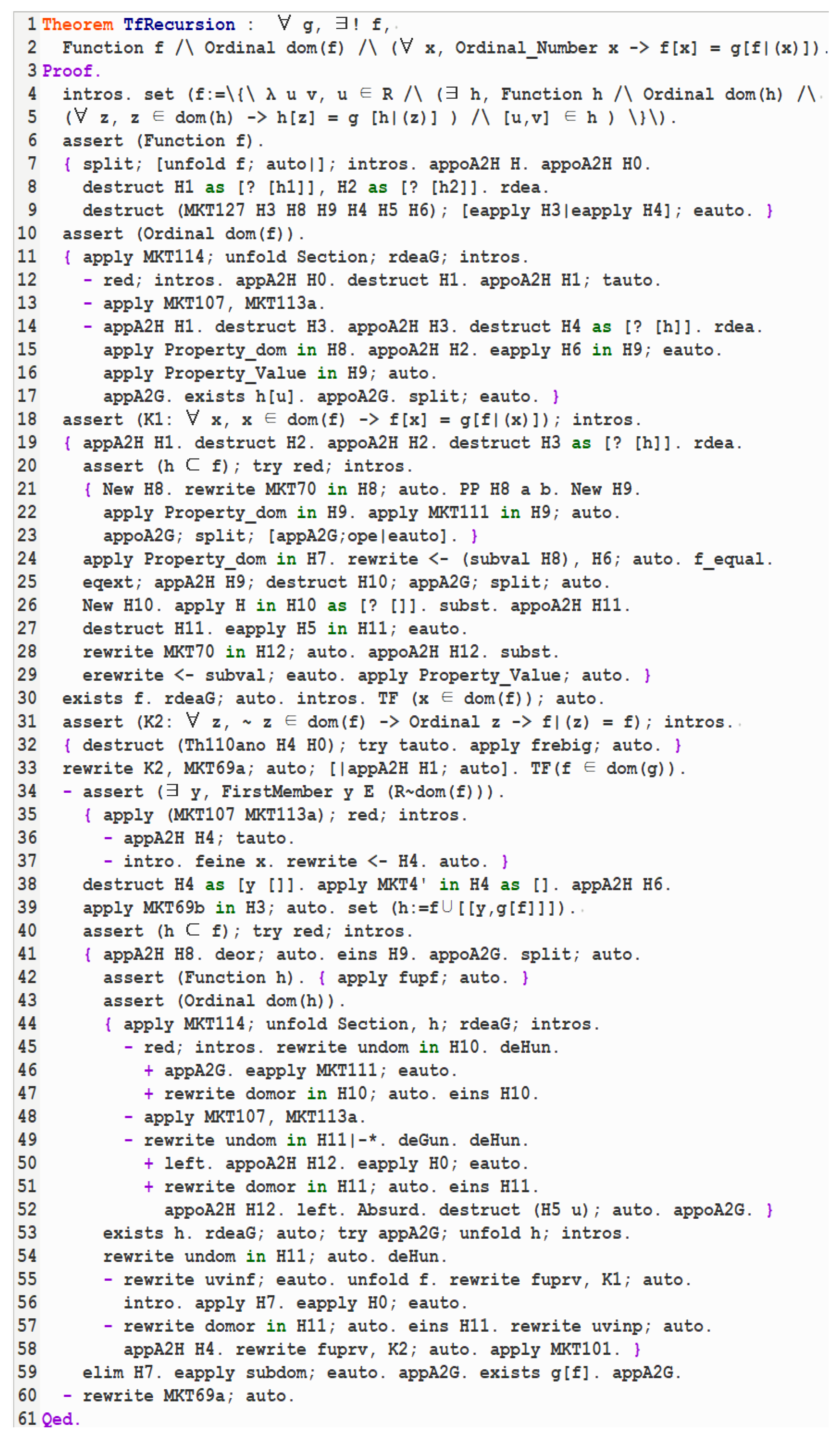
Theorem 1.
For each g there is a unique function f such that the is an ordinal and for each ordinal number.
The formalization of the theorem is expressed directly in Rocq as follows:
- Theorem TfRecursion : ∀ g, ∃! f,
- Function f /\ Ordinal dom(f) /\ (∀ x, Ordinal_Number x -> f[x] = g[f|(x)]).
Proof.
Uniqueness is easy to prove, and the following contents focus on existence. We first construct a ordered pair class f as follows, and prove that f is exactly what is required.
and there is a function h such that its domain is an ordinal, for z in the domain of h and
Let be the elements of f, then there exists functions with domain ordinal, that satisfy and for any ordinal number x and . According to Property 4, we have or . For the former case we can get that then since is a function. For the latter case, the same reasoning applies, so we have ; thus, f is a function.
According to Property 3, is an ordinal if is an E-section of R. As the construction of f, is a subclass of R. We can get E well-orders R by Property 1 and Property 2.
Then we discuss ordinal number x in two cases.
Case 1 (): We have in this case. Next, it can be inferred that by the construction of f , and there is a function h, whose properties are described above. We can get then and . Hence this conclusion is proved in this case.
Case 2 (): We have in this case. This case only requires proof of , that is . Assume to the contrary that it is. Supposing , there is a E-first member y of , and then we construct a new class . It is not difficult to prove that h is a function and its domain is an ordinal. In addition, we get that for so , which is in contradiction with . Therefore, this theorem is proven. □
4.3. Recursion Theorem on Natural Numbers
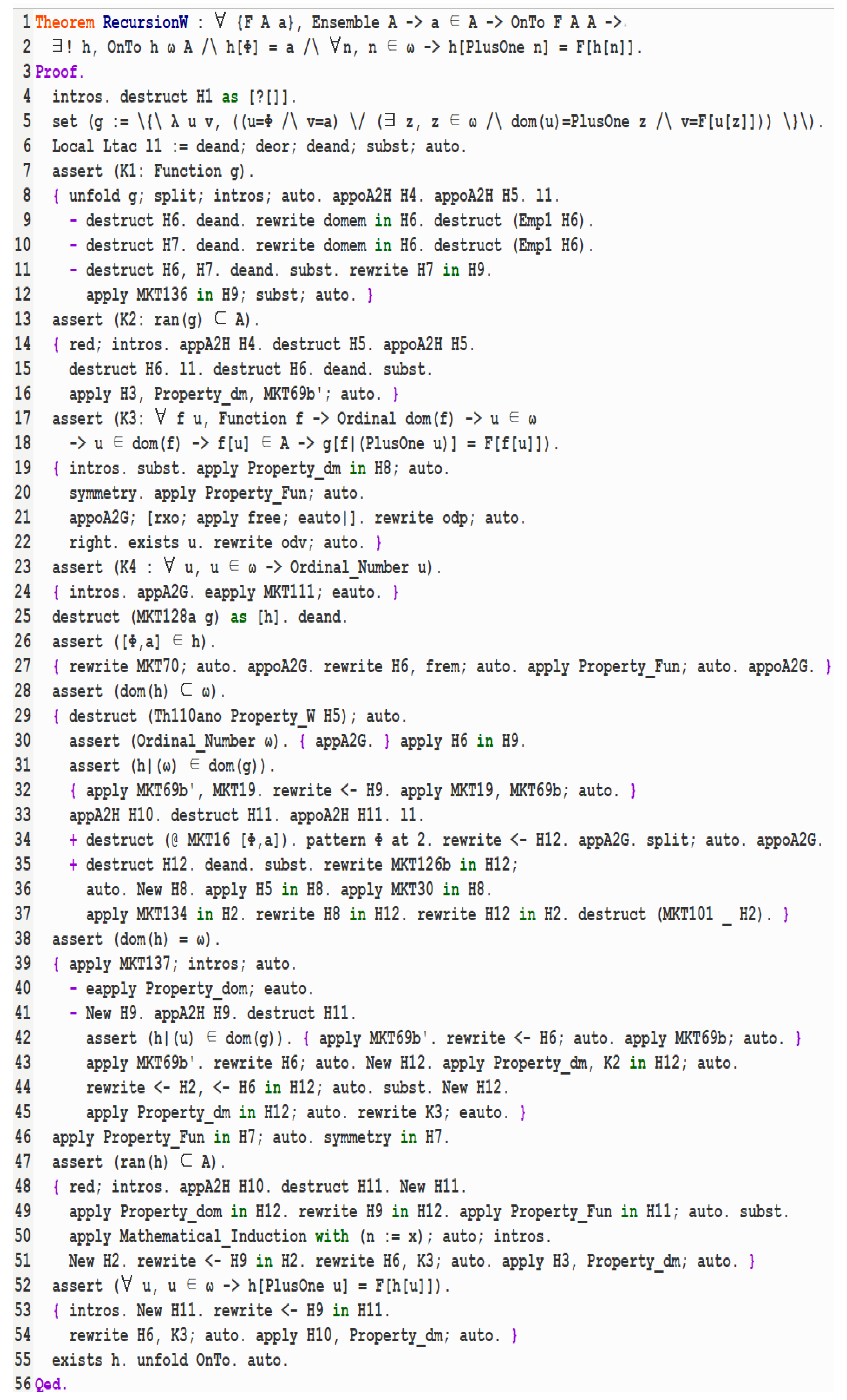
Theorem 2.
A is a set, a is the element of A, and function F is from A to A, then there is a unique function h which is from W to A, such that and
The formalization of the theorem is expressed directly in Rocq as follows:
- Theorem RecursionW: ∀ F A a, Ensemble A -> a ∈ A -> OnTo F A A ->
- ∃! h, OnTo h W A /\ h[Ø] = a /\ ∀n, n ∈ W -> h[PlusOne n] = F[h[n]].
Proof.
Uniqueness is easy to prove, and the following contents focus on existence. We first construct a ordered pair class g as follows.
Dom(u) is successor of natural number z and Let be the elements of g. For , , if not, then it cause the contradiction that ∅ is equal to the successor of a class. For another case, then there exists integer numbers whose successors of the two are equal, then . Moreover, we have , so g is a function.
By the construction of g, we can get that and any function f, whose domain is an ordinal, has the following properties:
According to Theorem 1, there is a function h, whose domain is an ordinal, such that for every ordinal number x. We can prove , and further we get by Mathematical Induction. By the properties of h, we can obtain . At last, by the construction of g we can get . Hence h is the function desired in the theorem. □
The formalizations of Transfinite Recursion Theorem and Recursion Theorem on natural numbers have completed, and the specific details of formal proof can be found in the appendix.
5. Machine Proof System of Analysis
The machine proof system of analysis is strictly following Landau’s "Foundations of Analysis". Starting from the Peano axioms, natural numbers (positive integers), fractions (positive), and rational numbers/integers (positive) are defined in order. The positive real numbers (called "Cut" in this book) are defined by Dedekind cut, and furthermore, adding negative real numbers and 0 to construct all real numbers. Finally, defining complex numbers by real number pairs and then the whole number system theory is realized naturally. Overall, "Foundations of Analysis" defines real numbers through construction rather than a series of axioms, and introduces the Dedekind fundamental theorem instead of admitting it as an axiom. The formalization of this book is sufficient as the basis in most areas of analysis.
5.1. Natural Nnumbers
To unify with it, we first define ’1’ and the set of positive natural numbers, which are formally described as follows.
- Definition One := PlusOne Ø.
- Definition Nat := W ̃ [Ø].
The successor function of positive natural numbers is formally described as follows:
- Definition Nsuc := \{\ λ u v, u ∈ Nat /\ v = PlusOne u \}\.
- Notation " x+ " := Nsuc[x](at level 0).
This further proves the mathematical induction method of positive natural numbers, which is formally described as follows:
- Theorem MathInd : ∀ P : Class -> Prop,
- P One -> (∀ k, k ∈ Nat -> P k -> P k+) -> (∀ n, n ∈ Nat -> P n).
Finally, provide a formal proof of the recursion theorem for positive natural numbers, as well as a function for constructing recursive operations.
- Theorem RecursionNex : {F A a}, Ensemble A -> a ∈ A -> OnTo F A A ->
- ∃ h, OnTo h Nat A /\ h[One] = a /\ ∀ n, n ∈ Nat -> h[n+] = F[h[n]].
- Theorem RecursionNun : ∀ h1 h2 F A a,
- OnTo h1 Nat A -> h1[One] = a -> (∀ n, n ∈ Nat -> h1[n+] = F[h1[n]]) ->
- OnTo h2 Nat A -> h2[One] = a -> (∀ n, n ∈ Nat -> h2[n+] = F[h2[n]]) -> h1 = h2.
- Definition NArith F a :=
- ∩ \{ λ h, OnTo h Nat Nat /\ h[One] = a /\ ∀ n, n ∈ Nat -> h[n+] = F[h[n]] \}.
By using the above function, one only needs to provide a function from Nat to Nat, as well as a positive natural number, to obtain the corresponding recursive function, because recursive functions are unique. From this, we can proceed to related contents of the natural number part. Starting with the formal proof of the Peano axioms as follows.
- Theorem FAA1 : One ∈ Nat.
- Theorem FAA2 : ∀ x y, x ∈ Nat -> y ∈ Nat -> x = y -> x+ = y+.
- Theorem FAA3 : ∀ x, x ∈ Nat -> x+ <> One.
- Theorem FAA4 : ∀ x y, x ∈ Nat -> y ∈ Nat -> x+ = y+ -> x = y.
- Theorem FAA5 : ∀ M, M ⊂ Nat -> One ∈ M -> (∀ u, u ∈ M -> u+ ∈ M) -> M = Nat.
The formal definition of natural number addition and its correctness verification are as follows.
- Definition addN := λ m, NArith Nsuc m+.
- Notation " x + y " := (addN x)[y].
- Fact addnT : ∀ {n}, n ∈ Nat ->
- OnTo (addN n) Nat Nat /\ n + One = n+ /\ ∀ m, m ∈ Nat -> n + m+ = (n + m)+.
Furthermore, we provide the formal definition of natural number subtraction and verify its correctness.
- Definition minN x y := ∩ \{ λ z, z ∈ Nat /\ x = y + z \}.
- Notation " x - y " := (minN x y).
- Fact MinNUn : ∀ {x y z}, x ∈ Nat -> y ∈ Nat -> z ∈ Nat -> x + y = z -> y = z - x.
- Fact MinNEx : ∀ {x y}, y > x -> x ∈ Nat -> y ∈ Nat -> x + (y - x) = y.
Finally, we provide the formal definition of natural number multiplication and verify its correctness.
- Definition mulN := λ m, NArith (addN m) m.
- Notation " x · y " := (mulN x)[y](at level 40).
- Fact mulNT : ∀ {n}, n ∈ Nat ->
- OnTo (mulN n) Nat Nat /\ n · One = n /\ ∀ m, m ∈ Nat -> n · m+ = (n · m) + n.
5.2. Fractions and Rational Numbers
Fractions are composed of ordered pairs of natural numbers, that is, fractions set is the cartesian product of the set of natural numbers with itself. Related definitions and properties of fractions are formally described as follows.
- (* Fractions set, Numerator and Denominator *)
- Definition FC := Nat × Nat.
- Notation " p 1 " := (First p)(at level 0) : FC_scope.
- Notation " p 2 " := (Second p)(at level 0) : FC_scope.
- (* Relation(~,>,<) *)
- Definition eqv f1 f2 := (f11 · f22)%Nat = (f21 · f12)%Nat.
- Notation " f1 ̃ f2 " := (eqv f1 f2): FC_scope.
- Definition gtf f1 f2 := (f11 · f22 > f21 · f12)%Nat.
- Notation " x > y " := (gtf x y) : FC_scope.
- Definition ltf f1 f2 := (f11 · f22 < f21 · f12)%Nat.
- Notation " x < y " := (ltf x y) : FC_scope.
- (* Operation(+,-,·,÷) *)
- Definition addF f1 f2 := [f11 · f22 + f21 · f12, f12 · f22]%Nat.
- Notation "f1 + f2" := (addF f1 f2) : FC_scope.
- Definition minF f1 f2 := [(f11 · f22) - (f21 · f12), f12 · f22]%Nat.
- Notation "f1 - f2" := (minF f1 f2) : FC_scope.
- Definition mulF f1 f2 := [f11 · f21, f12 · f22]%Nat.
- Notation " f1 · f2 " := (mulF f1 f2)(at level 40) : FC_scope.
- Definition divF f1 f2 := f1 · ([f22, f21]).
- Notation "f1 / f2" := (divF f1 f2) : FC_scope.
A rational number is a class composed of all equivalent fractions of a certain fraction. Related definitions and properties of rational numbers are formally described as follows.
- (* Rational Numbers *)
- Definition rC := \{λ S, ∃ F, F ∈ FC /\ S = \{λ f, f ∈ FC /\ f ̃ F \} \}%FC.
- (* Relation(>,<) *)
- Definition gtr r1 r2 := ∀ f1 f2, f1 ∈ r2 -> f2 ∈ r1 -> (f2 > f1)%FC.
- Notation " x > y " := (gtr x y) : rC_scope.
- Definition ltr r1 r2 := ∀ f1 f2, f1 ∈ r1 -> f2 ∈ r2 -> (f1 < f2)%FC.
- Notation " x < y " := (ltr x y) : rC_scope.
- (* Operation(+,-,·,÷) *)
- Definition addr r1 r2 :=
- \{ λ f, f ∈ FC /\ ∃ f1 f2, f1 ∈ r1 /\ f2 ∈ r2 /\ f ̃ (f1 + f2) \}%FC.
- Notation "r1 + r2" := (addr r1 r2) : rC_scope.
- Definition minr r1 r2 :=
- \{ λ f, f ∈ FC /\ ∃ f1 f2, f1 ∈ r1 /\ f2 ∈ r2 /\ f ̃ (f1 - f2) \}%FC.
- Notation " r1 - r2 " := (minr r1 r2) : rC_scope.
- Definition mulr r1 r2 :=
- \{ λ f, f ∈ FC /\ ∃ f1 f2, f1 ∈ r1 /\ f2 ∈ r2 /\ f ̃ (f1 · f2) \}%FC.
- Notation " r1 · r2 " := (mulr r1 r2)(at level 40) : rC_scope.
- Definition divr r1 r2 :=
- \{ λ f, f ∈ FC /\ ∃ f1 f2, f1 ∈ r1 /\ f2 ∈ r2 /\ f ̃ (f1 / f2) \}%FC.
- Notation " r1 / r2 " := (divr r1 r2)(at level 40) : rC_scope.
This part presents the definition of fractions and establishes a direct connection with rational numbers through the concept of equivalence classes. Additionally, we prove the Archimedean property for rational numbers.
5.3. Cuts
Landau’s definition of Cuts(positive real numbers) refers to Dedekind cut. A rational number set M is a the cut (positive real number), if it satisfies these properties as follows:
(1) M is not empty and there exists rational numbers don’t belong to M;
(2) M contains all rational numbers smaller than any element in M;
(3) With every number it contains, the M also contains a greater one.
Related definitions and properties of cuts are formally described as follows.
- (* Cuts, Lower Number and Upper Number *)
- Definition CC := \{λ S, S ⊂ rC /\ (S <> Ø /\ ∃ r, r ∈ rC /\ ̃ r ∈ S) /\
- (∀ r1 r2, r1 ∈ S -> r2 ∈ rC -> r2 < r1 -> r2 ∈ S) /\
- (∀ r1, r1 ∈ S -> ∃ r2, r2 ∈ S /\ r1 < r2) \}%rC.
- Definition Num_L r c := r ∈ c.
- Definition Num_U r c := ̃ r ∈ c.
- (* Relation(>,<) *)
- Definition gtc c1 c2 := ∃ r, Num_L r c1 /\ Num_U r c2.
- Notation " x > y " := (gtc x y) : CC_scope.
- Definition ltc c1 c2 := ∃ r, Num_L r c2 /\ Num_U r c1.
- Notation " x < y " := (ltc x y) : CC_scope.
- (* Operation(+,-,·,1,÷,√) *)
- Definition addc c1 c2 :=
- \{λ c, ∃ r1 r2, Num_L r1 c1 /\ Num_L r2 c2 /\ c = (r1 + r2) \}%rC.
- Notation "c1 + c2" := (addc c1 c2) : CC_scope.
- Definition minc c1 c2 := \{λ r, ∃ r1 r2,
- Num_L r1 c1 /\ r2 ∈ rC /\ Num_U r2 c2 /\ r2 < r1 /\ r = (r1 - r2) \}%rC.
- Notation " x - y " := (minc x y) : CC_scope.
- Definition mulc c1 c2 :=
- \{λ c, ∃ r1 r2, Num_L r1 c1 /\ Num_L r2 c2 /\ c = (r1 · r2)%rC \}.
- Notation " c1 · c2 " := (mulc c1 c2)(at level 40) : CC_scope.
- Definition recC c := \{ λ r, r ∈ rC /\
- ∃ r0, r0 ∈ rC /\ Num_U r0 c /\ (~ LNU r0 c) /\ r = (Ntor One) / r0) \}.
- Notation " c1 / c2 " := c1 · (recC c2).(at level 40) : CC_scope.
- Definition Sqrt_C c := \{ λ r, r ∈ rC /\ (rtoC r) · (rtoC r) < c \}.
- Notation " √ c " := (Sqrt_C c)(at level 0) : CC_scope.
This part presents the construction method of cuts, moreover, we prove the existence of irrational numbers().
5.4. Real Numbers
Every cut is a positive real number, and each positive real number corresponds to a negative real number. At the same time, we define the 0 distinct from positive real number and negative real number, then the specific implementation is as follows.
(1) ∅ represents 0.
(2) represents positive real number, where u is a cut.
(3) represents negative real number, where u is a cut.
Related definitions and properties of real numbers are formally described as follows.
- (* 0, positive, negative, real numbers class and value of real numbers *)
- Definition zero := Ø.
- Notation " 0 " := zero : RC_scope.
- Definition PRC := \{\ λ u v, u ∈ CC /\ v = 0 \}\.
- Definition NRC := \{\ λ u v, u = 0 /\ v ∈ CC \}\.
- Definition RC := PRC ∪ [0] ∪ NRC.
- Notation " p 1 " := (First p)(at level 0) : RC_scope.
- Notation " p 2 " := (Second p)(at level 0) : RC_scope.
- (* Relation(>,<) *)
- Definition gtR r1 r2 := (r2 ∈ PRC /\ r1 ∈ PRC /\ (r21 < r11)%CC) \/
- (r2 = 0 /\ r1 ∈ PRC) \/ (r2 ∈ NRC /\ r1 ∈ PRC) \/
- (r2 ∈ NRC /\ r1 = 0) \/ (r2 ∈ NRC /\ r1 ∈ NRC /\ (r12 < r22)%CC).
- Notation " x > y " := (gtR x y) : RC_scope.
- Definition ltR r1 r2 := (r1 ∈ PRC /\ r2 ∈ PRC /\ (r11 < r21)%CC) \/
- (r1 = 0 /\ r2 ∈ PRC) \/ (r1 ∈ NRC /\ r2 ∈ PRC) \/
- (r1 ∈ NRC /\ r2 = 0) \/ (r1 ∈ NRC /\ r2 ∈ NRC /\ (r22 < r12)%CC).
- Notation " x < y " := (ltR x y) : RC_scope.
- (* Operation(||,+,-,·,÷,√) *)
- Definition AbsR := \{\ λ r z, r ∈ RC /\
- (r ∈ NRC -> z = [r2,0]) /\ (r ∈ PRC -> z = r) /\ (r = 0 -> z = 0) \}\.
- Notation " | X | " := (AbsR[X])(at level 10) : RC_scope.
- Definition addR a := \{\ λ b c, b ∈ RC /\
- (a ∈ PRC -> b ∈ PRC -> c = [a1 + b1,0]) /\
- (a ∈ NRC -> b ∈ NRC -> c = [0, a2 + b2]) /\ (a = 0 -> c = b) /\
- (b = 0 -> c = a) /\ (a ∈ PRC -> b ∈ NRC -> (a1 = b2 -> c = 0) /\
- (gtc a1 b2 -> c = [a1 - b2,0]) /\ (ltc a1 b2 -> c = [0,b2 - a1])) /\
- (a ∈ NRC -> b ∈ PRC -> (a2 = b1 -> c = 0) /\
- (gtc a2 b1 -> c = [0,a2 - b1]) /\ (ltc a2 b1 -> c = [b1 - a2,0])) \}\.
- Notation "x + y" := ((addR x) [y]) : RC_scope.
- Definition minR := \{\ λ a b, a ∈ RC /\
- (a ∈ PRC -> b = [0,a1]) /\ (a ∈ NRC -> b = [a2,0]) /\ (a = 0 -> b = 0) \}\.
- Notation "- x" := (minR[x]) : RC_scope.
- Definition MinR x y := x + (-y).
- Notation "x - y" := MinR x y : RC_scope.
- Definition mulR a := \{\ λ b c, b ∈ RC /\ (a ∈ PRC -> b ∈ PRC -> c = [a1·b1,0]) /\
- (a ∈ NRC -> b ∈ NRC -> c = [a2·b2,0]) /\ (a ∈ PRC -> b ∈ NRC -> c = [a1·b2,0]) /\
- (a ∈ NRC -> b ∈ PRC -> c = [a2·b1,0]) /\ (a = 0 -> c = 0) /\ (b = 0 -> c = 0) \}\.
- Notation " x · y " := ((mulR x) [y])(at level 40) : RC_scope.
- Definition divR a := \{\ λ b c, b ∈ RC /\ b <> 0 /\
- (b ∈ PRC -> c = a · [(recC b1),0]) /\ (b ∈ NRC -> c = a · [0,(recC b2)]) \}\.
- Notation " x / y " := ((divR x) [y]) : RC_scope.
- Definition Sqrt_R := \{\ λ a b, a ∈ RC /\ ̃ a ∈ NRC /\
- (a ∈ PRC -> b = [(√ (a1))%CC, 0]) /\ (a = 0 -> b= 0) \}\.
- Notation " √ a " := (Sqrt_R [a])(at level 0): RC_scope.
This part presents how to extend from cuts to real numbers and further realize their various order relations and operations. Meanwhile, we prove the Dedekind fundamental theorem in last.
5.5. Complex Numbers
Complex numbers are composed of ordered pairs of real numbers that is similar to the relationship between fractions and natural numbers. Related definitions and properties of fractions are formally described as follows.
- (* Complex numbers set, Real part and Imaginary part *)
- Definition cC := RC × RC.
- Notation " p 1 " := (First p)(at level 0) : cC_scope_.
- Notation " p 2 " := (Second p)(at level 0) : cC_scope.
- (* Operation(+,-,·,÷,¯,||) *)
- Definition addC x y := [x1 + y1, x2 + y2]%RC.
- Notation "x + y" := (addC x y) : cC_scope.
- Definition minC x y := [x1 - y1, x2 - y2]%RC.
- Notation " x - y " := (minC x y) : cC_scope.
- Definition mulC x y := [x1 · y1 - x2 · y2, x1 · y2 + x2 · y1]%RC.
- Notation " x · y " := (mulC x y) : cC_scope.
- Definition Out_1 x := ((x1) / (Square_cC x))%RC.
- Definition Out_2 x := (- ((x2) / (Square_cC x)))%RC.
- Definition DivC x y:= [(y1) / (Square_cC y), (-x2)/ (Square_cC x)] · x.
- Notation " x / y " := (DivC x y) : cC_scope.
- Definition Conj x := [x1, (-x2)]%RC.
- Notation " x $^{-}$ " := (Conj x)(at level 0) : cC_scope.
- Definition Abs_cC x := √((x1 · x1) + (x2 · x2)).
- Notation " | x | " := (Abs_cC x) : cC_scope.
All content of the complex numbers part has also been fully formalized, but we will not elaborate on it in detail here because of space limitations. Researchers who are interested can refer to our source code for more information.
6. Conclusions and Future Work
We completed the formalization of the machine proof system of analysis based on Morse-Kelley axiomatic set theory. Firstly, we introduce the machine proof system of Morse-Kelley axiomatic set theory that is concise while remaining comprehensive enough for analysis. This content covers not only our formalization work but also highlights the distinctions and advantages of our approach relative to prior research. Next, we provide the proof for the Transfinite Recursion Theorem key conclusion within the MK system. Furthermore, leveraging this theorem, we prove the Recursion Theorem for natural numbers, the critical result for defining operations on natural numbers. Finally, we present the implementation details of the machine proof system designed for analysis, which encompasses natural numbers, fractions, cuts, real numbers and complex numbers. This system adheres to the framework of Landau’s "Foundations of Analysis" and adopts MK as its foundational descriptive language. All proofs undergo verification in Rocq to ensure rigor and correctness, and we supplement any missing proof details to enhance the formal system’s completeness.
In the future, we will complete the formalization of deeper contents of this theory such as calculus, point set topology and abstract algebra. Meanwhile, We will complete the extension to previous work. Furthermore, this work can be promoted to undergraduate teaching to help students better understand the specific contents on axiomatic set theory and mathematical analysis.
Author Contributions
Conceptualization, Y.G.; methodology, Y.G. and Y.F.; software, Y.F.; validation, Y.F.; formal analysis, Y.G. and Y.F.; investigation,Y.G. and X.M.; resources, Y.F.; data curation, Y.G.; writing—original draft preparation, Y.G. and Y.F.; writing—review and editing, Y.G and Y.F.; visualization, X.M.; supervision, Y.F.; project administration, X.M.; funding acquisition, Y.F. All authors have read and agreed to the published version of the manuscript.
Funding
This research was funded by National Natural Science Foundation (NNSF) of China under Grant 62388101 and 62476028.
Acknowledgments
We are grateful to the anonymous reviewers, whose comments greatly helped to improve the presentation of our research in this article.
Conflicts of Interest
The authors declare no conflict of interest.
Appendix A.
The formal proof of Transfinite Recursion Theorem is shown in Figure A1.
Figure A1.
Formal proof of Transfinite Recursion Theorem.
Appendix B.
The formal proof of Recursion Theorem on natural numbers is shown in Figure A2.
Figure A2.
Formal proof of Recursion Theorem on natural numbers.
References
- Beeson, M. Mixing computations and proofs. J. Formaliz. Reason. 2016, 9, 71–99.
- Van Benthem Jutting, L.S. Checking Landau’s "Grundlagen" in the AUTOMATH System. Ph.D. Thesis, Eindhoven University of Technology, Eindhoven, The Netherlands, 1977.
- Bertot, Y.; Castéran, P. Interactive Theorem Proving and Program Development. Coq’Art: The Calculus of Inductive Constructions; Texts in Theoretical Computer Science; Springer: Berlin/Heidelberg, Germany, 2004.
- Bernays, P.; Fraenkel, A. A. Axiomatic Set Theory. North Holland Publishing Company:Amsterdam, Netherlandish, 1958.
- Boldo, S.; Lelay, C.; Melquiond, G. Coquelicot: A User-Friendly Library of Real Analysis. Math. Comput. Sci. 2015, 9, 41–62.
- Brown, C.E. Faithful Reproductions of the Automath Landau Formalization. Technical Report. 2011. Available online: https://www.ps.uni-saarland.de/Publications/documents/Brown2011b.pdf (accessed on 28 July 2018).
- Chlipala, A. Certified Programming with Dependent Types: A Pragmatic Introduction to the Coq Proof Assistant; MIT Press: Cambridge, MA, USA, 2013.
- The Coq Development Team. The Coq Proof Assistant Reference Manual (Version 8.9.1). 2019. Available online: https://coq.inria.fr/distrib/8.9.1/refman/ (accessed on 4 August 2019).
- Courant, R.; John, F.; Blank, A. A., et al. Introduction to Calculus and Analysis; Interscience Publishers: New York, USA, 1965.
- Coquand, T.; Paulin, C. Inductively Defined Types. In Lecture Notes in Computer Science, Proceedings of the International Conference on Computer Logic (COLOG 1988), 12–16 December 1988; Springer: Berlin/Heidelberg, Germany, 1990; Volume 417, pp. 50–66.
- Coquand, T.; Huet, G. The calculus of constructions. Inf. Comput. 1988, 76, 95–120.
- Cruz-Filipe, L.; Marques-Silva, J.; Schneider-Kamp, P. Formally verifying the solution to the Boolean Pythagorean triples problem. J. Autom. Reason. 2019, 63, 695–722.
- Fu, Y.; Yu, W. A Formalization of Properties of Continuous Functions on Closed Intervals. In Lecture Notes in Computer Science, Proceedings of the International Congress on Mathematical Software(ICMS 2020), Braunschweig, Germany, 13–16 July 2020; Bigatti A., Carette J.,Joswig M., de Wolff T., Eds; Springer: Cham, Switzerland, 2020; Volume 12097, pp. 272–280.
- Fu, Y.; Yu, W. Formalizing equivalence between real number completeness and intermediate value theorem. China Automation Congress(CAC 2021), Beijing, China, 22–24 October 2021; Volume 12097, pp. 5337–5340.
- Fu, Y.; Yu, W. Formalizing Calculus without Limit Theory in Coq. Mathematics 2021, 9, 1377, . [CrossRef]
- Gonthier, G.; Asperti, A.; Avigad, J.; Bertot, Y.; Cohen, C.; Garillot, F.; Roux, S.L.; Mahboubi, A.; O’Connor, R.; Biha, S.O.; et al. Machine-checked proof of the Odd Order Theorem. In Lecture Notes in Computer Science, Proceedings of the Interactive Theorem Proving 2013 (ITP 2013), Rennes, France, 22–26 July 2013; Blazy, S., Paulin-Mohring, C., Pichardie, D., Eds; Springer: Berlin/Heidelberg, Germany, 2013; Volume 7998, pp. 163–179.
- Geuvers, H.; Niqui, M. Constructive reals in Coq: Axioms and categoricity. Types for Proofs and Programs(TYPES 2000), Durham, UK, 8-12 December, 2000; Goos, G., Hartmanis, J., van Leeuwen, J., Eds; Springer: Berlin/Heidelberg, Germany, Volume 2277, pp. 79–95.
- Gonthier, G. Formal proof—The Four Color Theorem. Not. Am. Math. Soc. 2008, 55, 1382–1393.
- Grabiner, J.V. Who gave you the epsilon? Cauchy and the origins of rigorous calculus. Am. Math. Mon. 1983, 90, 185–194.
- Grimm, J. Implementation of Bourbaki’s mathematics in Coq: Part two, from natural to real numbers. Journal of Formalized Reasoning. 1983, 90, 185–194.
- Gu, R.; Shao, Z.; Chen, H., et al. CertiKOS: An Extensible Architecture for Building Certified Concurrent OS Kernels. Proc of the USENIX Symp. Operating Syst. Design Implement,Savannah, GA, USA, 2-4 November,2016, USENIX Association: Berkeley, USA, 2016; pp. 653–669.
- Guidi, F. Verified Representations of Landau’s "Grundlagen" in the lambda-delta Family and in the Calculus of Constructions. J. Formaliz. Reason. 2016, 8, 93–116.
- Halmos, P. R. Naive Set Theory. Springer-Verlag: New York, USA, 1974.
- Hales, T. Formal proof. Not. Am. Math. Soc. 2008, 55, 1370–1380.
- Hales, T.; Adams, M.; Bauer, G.; Dang, T.D. A Formal Proof of the Kepler Conjecture. Forum of Mathematics, Pi; Cambridge University Press: Cambridge, UK, 2017; Volume 5, pp. 1–29.
- Harrision, J. Formal proof—Theory and practice. Not. Am. Math. Soc. 2008, 55, 1395–1406.
- Heijenoort J. V. From Frege to Gödel: A Source Book in Mathematical Logic. Harvard University Press : Cambridge, UK, 1967.
- Heule, M.; Kullmann, O.; Marek, V. Solving and Verifying the Boolean Pythagorean Triples Problem via Cube-and-Conquer. In Lecture Notes in Computer Science, Proceedings of the Theory and Applications of Satisfiability Testing 2016(SAT 2016), Bordeaux, France, 5–8 July 2016; Creignou, N., Le Berre, D., Eds; Springer: Cham, Switzerland, 2016; Volume 9710, pp. 228–245.
- Harrison, J.; Urban, J.; Wiedijk, F. History of Interactive Theorem Proving. Handbook of the History of Logic: Computational Logic. 2014, 9, 135–214.
- Jiang, N.; Li, Q; Wang, L; et al. Overview on Mechanized Theorem Proving. Journal of software 2020, 31(1), 82–112.
- Kelley, J. L. General Topology. Springer-Verlag: New York, USA, 1955.
- Kirst, D.; Smolka, G. Categoricity Results for Second-Order ZF in Dependent Type Theory. In Lecture Notes in Computer Science, Proceedings of the Interactive Theorem Proving 2017 (ITP 2017), Brasília, Brazil, September 26–29, 2017; Ayala-Rincón, M., Muñoz, C.A., Eds; Springer: Cham, 2017; Volume 10499, pp. 304–318.
- Landau, E. Foundations of Analysis: The Arithmetic of Whole, Rational, Irrational, and Complex Numbers; Chelsea Publishing Company: New York, NY, USA, 1966.
- Luo, Z. ECC, an extended calculus of constructions. In Proceedings of the Fourth Annual Symposium on Logic in Computer Science, California, USA, 5–8 June 1989; IEEE Press: Piscataway, NJ, USA, 1989; pp. 386–395.
- Morse, A. P. A Theory of Sets. Academic: New York, USA, 1965.
- Vivant, C. Thèoréme Vivamt; Grasset: Prais, France, 2012.
- Voevodsky, V. Univalent Foundations of Mathematics; Beklemishev, L., De Queiroz, R., Eds; Springer: Berlin/Heidelberg, Germany, 2011; Volume 6642, p. 4.
- Wiedijk, F. Formal proof—Getting started. Not. Am. Math. Soc. 2008, 55, 1408–1414.
- Wang, J.; Zhan, N; Feng, X; et al. Overview of Formal Methods. Journal of software 2019, 30(1), 33–61.
- Yu, W.; Sun, T.; Fu, Y. Machine Proof System of Axiomatic Set Theory; Science Press: Beijing, China, 2020.
- Yu, W.; Fu, Y.; Guo. L. Machine Proof System of Analysis of foundatios; Science Press: Beijing, China, 2022.
- Zorich, V. A.; Paniagua, O. Mathematical analysis; Springer: New York, USA, 2016.
Disclaimer/Publisher’s Note: The statements, opinions and data contained in all publications are solely those of the individual author(s) and contributor(s) and not of MDPI and/or the editor(s). MDPI and/or the editor(s) disclaim responsibility for any injury to people or property resulting from any ideas, methods, instructions or products referred to in the content. |
© 2025 by the authors. Licensee MDPI, Basel, Switzerland. This article is an open access article distributed under the terms and conditions of the Creative Commons Attribution (CC BY) license (http://creativecommons.org/licenses/by/4.0/).
Copyright: This open access article is published under a Creative Commons CC BY 4.0 license, which permit the free download, distribution, and reuse, provided that the author and preprint are cited in any reuse.


