Submitted:
25 November 2025
Posted:
25 November 2025
You are already at the latest version
Abstract
In traditional portfolio optimization models, prediction errors of excess returns in asset selection can lead to performance degradation. This paper employs the Transformer deep learning model to predict the return rates of candidate assets, aiming to enhance the accuracy of return predictions and thereby improve portfolio performance. Using the CSI 800 Index’s constituent stocks as candidate assets, we conduct 72-period rolling investments and compare the results with LSTM and SVR models. The empirical results demonstrate the superiority of the Transformer model in improving predictive accuracy and portfolio model performance.
Keywords:
portfolio optimization
; deep learning
; mean-variance model
; transformer model
1. Introduction
Due to the influence of macroeconomic conditions, investor psychology, government policies, and other factors, financial asset prices often exhibit sharp fluctuations, high noise, and characteristics such as nonlinearity, instability, and complexity [1]. Scholars have attempted to address problems that traditional statistical methods cannot solve by applying artificial intelligence methods based on machine learning, aiming to provide descriptive, explanatory, and predictive models for financial market analysis and investment decision-making. These models can identify important patterns from large volumes of unstructured financial data [2].
Traditional machine learning methods have been widely applied in financial asset prediction, especially in time series forecasting. Among them, support vector regression (SVR) and artificial neural networks (ANN) are the most commonly used methods. In recent years, deep learning has emerged rapidly in the field of machine learning, particularly gaining attention in financial forecasting. Due to the evolving market landscape, deep learning models have increasingly become mainstream approaches capable of accurately identifying complex patterns in financial data [3], thus demonstrating better performance than classic machine learning methods [4]. Long short-term memory networks (LSTM), convolutional neural networks (CNN), and deep multilayer perceptron (DMLP) are among the most widely used deep learning models in finance. LSTM is particularly suited for time series forecasting, while DMLP and CNN are better suited for classification tasks requiring feature extraction [5].
In 1952, the mean-variance (MV) model was proposed [6]. This model quantifies asset return optimization by minimizing risk through the mean-variance or mean-covariance matrix of returns, thereby constructing a theoretically optimal investment portfolio [7]. The MV model has been widely used by both investors and researchers to understand the construction of various investment portfolios and holds significant theoretical and practical implications. However, the MV model is extremely sensitive to input prediction errors. The prediction errors of excess returns (differences between expected and actual returns or risk-adjusted returns) in asset selection may significantly degrade the performance of investment models [8,9]. Some researchers have explored using machine learning methods to predict returns of selected assets, aiming to improve predictive accuracy and thereby enhance portfolio model performance.
With the rapid development of machine learning, increasingly optimal deep learning models have continuously emerged. These models show greater potential in handling financial time series with long-term, cross-period dependencies, such as the recently popular Transformer model.
Based on existing research [10,11,12,13,14,15], this paper focuses on two main areas: (1) adopting the Transformer deep learning model to predict returns, and comparing its prediction results with LSTM and SVR models to evaluate its ability to predict excess returns of selected assets; (2) applying prediction results from the Transformer model in the traditional mean-variance model to construct a theoretically optimal investment portfolio, and comparing results with those from LSTM and SVR models to examine the model’s ability to improve portfolio performance.
2. Related Work
In recent years, deep learning methods have gained significant attention in financial forecasting and portfolio optimization. Compared with traditional approaches, deep neural networks can more effectively capture the nonlinear structures and complex dependencies embedded in financial time series, thereby improving the accuracy of asset return prediction [16,17]. Existing studies indicate that deep learning outperforms shallow models in cross-sectional stock return prediction and demonstrates stronger adaptability in practical portfolio construction [16,18]. Moreover, incorporating clustering techniques to enhance the modeling of stock similarity has been shown to improve prediction performance and promote more rational asset allocation [19]. Furthermore, end-to-end portfolio optimization frameworks based on deep architectures provide enhanced adaptability to dynamic market environments [20].
Within deep learning models, the development of attention mechanisms-particularly the Transformer architecture-has provided an effective means to model long-range dependencies in financial time series [21]. Recent research has explored the use of Transformers in asset price forecasting and risk identification, improving asset management accuracy through advanced temporal modeling [22,23]. Transformer-based models integrated with transaction graph information have also been applied to anti-money-laundering risk monitoring, demonstrating the potential of Transformers in fusing graph-structured financial data [24].
Beyond deterministic forecasting models, reinforcement learning has been widely adopted for dynamic investment strategy formulation. Through deep reinforcement learning, agents can continuously adjust portfolio strategies in response to market conditions to optimize long-term returns [25,26]. Studies show that such methods not only exhibit strong autonomous decision-making capabilities but also achieve better dynamic trade-offs between risk control and return maximization [27].
Graph neural networks and anomaly detection mechanisms have also emerged as important research directions in finance, particularly in corporate risk assessment and transaction fraud detection [28,29,30]. For instance, combining dynamic graph modeling with multi-head self-attention enables the effective identification of abnormal fluctuations in financial data, thereby enhancing early risk warning capabilities [31]. Under complex sequential and transactional data scenarios, improved sequence modeling methods provide more robust support for financial fraud detection [32].
Moreover, to enhance model interpretability and generalization, some studies have focused on structural-aware attention mechanisms, knowledge graph integration, causal inference, and regularization techniques [33,34,35]. These advancements not only enrich the expressive power of deep learning models but also improve their reliability in high-stakes financial applications [36,37].
In summary, deep learning models have developed rapidly and diversely in the fields of asset return prediction and portfolio optimization in recent years. Among them, Transformer-based models have gradually become mainstream due to their superior capability in sequence modeling. Building upon this body of research, this paper introduces the Transformer architecture into the traditional mean–variance portfolio optimization framework, aiming to improve return forecasting accuracy and thereby enhance overall portfolio performance.
3. Model Construction
3.1. Portfolio Construction
3.1.1. Single-Period Portfolio Construction
The framework for constructing a single-period portfolio is shown in Figure 1 on the next page. To construct a portfolio suitable for the next period, it is first necessary to use historical data of the candidate assets over a certain time window. Transformer, LSTM, and SVR are used respectively to predict the expected excess returns of each candidate asset in the next period. The predicted excess returns are then input into the MV model to construct the theoretically optimal portfolio.
The prediction of the expected excess return of each asset in the next period is a supervised learning task, also a regression problem. When using various models to make predictions, historical data of each asset and its relationship with future excess returns are required, as shown in Figure 2 on the next page. To predict the excess return at period , data from period t need to be used as explanatory variables. In addition, it is necessary to collect explanatory variable data from period to , as well as the corresponding target excess return data from period to t.
When training models like SVR, one can directly input the explanatory variables for one period and the corresponding next-period excess return. However, before training deep learning models like Transformer, it is necessary to extract subsequences of length m from the time series using a sliding window.
3.1.2. Multi-Period Portfolio Construction
When constructing multi-period portfolios, this paper adopts the commonly used sliding window approach for return prediction and portfolio research [38], as illustrated in Figure 3. To construct a portfolio for period , observable historical data from period to t are used to predict the excess return in period , and then the portfolio is constructed based on this prediction. To construct a portfolio for period , data from period to are used. The process continues in this manner.
3.2. Transformer Model
The Transformer model structure used in this paper is illustrated in Figure 4. First, the input explanatory variable sequence is expanded in dimensionality through a linear layer. Positional encodings are computed and added to the input sequence to represent the positional information of elements in the numerical sequence.
Next, the transformed input sequence is passed through N layers of Transformer encoder modules, where the output of each encoder layer serves as the input for the next layer.
Each encoder module consists of two parts. The first part is the multi-head self-attention mechanism, which is responsible for capturing the correlation and deep features within the input sequence. Each attention head learns different features. Dropout is applied within this part to prevent overfitting from future information leakage. The second part is a feedforward neural network, which integrates the outputs from the attention mechanism. Each part of the output undergoes residual connection and normalization.
Finally, the output of the last encoder module is passed through a linear layer for integration, resulting in the predicted sequence of excess returns.
3.3. MV Model
The MV model uses and to measure the returns and risks of each asset. By solving the optimization problem in Equation (1), the portfolio weights are adjusted to maximize returns and minimize risk, thereby obtaining the theoretically optimal portfolio.
Here, represents the expected excess return vector for n candidate assets, as provided by each prediction model; represents the variance-covariance matrix of expected returns, estimated using the historical excess return variance-covariance matrix of the assets; is the risk aversion coefficient of the investor; is an n-dimensional vector of ones; is the portfolio weight for asset i, with and each .
4. Empirical Analysis
4.1. Data Selection
This paper uses the constituent stocks of the CSI 800 Index as candidate assets, with a single-period investment horizon of one month. From January 2015 to December 2020, a total of 72 rolling investment periods are conducted. In each sliding window, the historical data length M is set to 30 months, and the input sequence length m for deep learning models is set to 12 months.
Since the CSI 800 Index constituents are adjusted semiannually, the candidate stocks also change accordingly. Stocks with missing or discontinuous historical data due to delisting, suspension, or other reasons are removed from the candidate pool in the corresponding period.
To predict the expected excess returns of candidate stocks, this paper uses 10 classic explanatory variables as shown in Table 1. For example, in the first investment period (January 2015), there are 507 candidate stocks. The explanatory variable data from June 2012 to December 2014 are shown in Table 2, and the first-level industry classifications are shown in Figure 5 (data source: Wind database) [39].
4.2. Return Prediction
Due to the high cost of training deep learning models, this paper performs two rounds of hyperparameter tuning using data from January 2014 to December 2017. The resulting models are then applied to the investment periods 2015–2017 and 2018–2020. The hyperparameter settings for each prediction model are summarized in Table 3.
RMSE and MAPE are used to evaluate the prediction accuracy of excess returns. The lower the value of these error metrics, the higher the model’s predictive performance.
Table 4 shows the prediction errors of the three models over the 72 investment periods. The results indicate the following:
(1) Based on RMSE, the SVR model has the lowest average prediction error at 0.115, followed by Transformer, and the LSTM model has the highest at 0.132.
(2) Based on MAPE, the Transformer model achieves the smallest average and standard deviation of prediction errors, at only 610 and 1998, respectively, while SVR and LSTM produce significantly larger errors than Transformer.
(3) The MAPE skewness values of all three models exceed 7, indicating a highly right-skewed distribution. This suggests that although the models perform well in most periods, extremely large errors occur in a few periods.
From this, it can be concluded that in predicting the excess returns of candidate stocks, the Transformer and SVR models exhibit relatively higher prediction accuracy, whereas the LSTM model performs relatively poorly.
4.3. Investment Performance of Portfolios Constructed Using the MV Model
This paper uses the variance-covariance matrix of the excess returns over the past 12 months of each candidate stock as the estimate of in the MV model. The risk aversion coefficient is set to 3. The predicted excess returns obtained from the three forecasting models—Transformer, LSTM, and SVR—are used as the input expected returns for the MV model to construct portfolios.
As shown in Figure 6 and Table 5, the Transformer model demonstrates superior performance in enhancing the investment effectiveness of the MV model.
The portfolio constructed using the Transformer and MV model achieved higher returns in four out of six years compared to the portfolios constructed using LSTM or SVR combined with the MV model. In five out of six years, it outperformed both the CSI 800 Index and the CSI 800 Equal-weighted Index. Among all portfolios, it achieved the highest cumulative return, annualized return, and Sharpe ratio, reaching 107.96%, 12.98%, and 0.46, respectively. In contrast, the portfolio based on SVR and MV attained a cumulative return of 53.02%, an annualized return of 7.35%, and a Sharpe ratio of 0.25. The portfolio based on LSTM and MV underperformed even the market benchmarks.
It is worth noting that the portfolios constructed using the MV model contained relatively few stocks. As shown in Figure 6, except for the first period of the Transformer-based portfolio which included 29 stocks, the number of stocks in all other periods did not exceed 13. Such compact portfolios are suitable not only for institutional investors but also for individual investors.

Table 6.
Number of Stocks in Portfolios Constructed Using the MV Model.
| Min | 25% Quantile | Median | 75% Quantile | Max | |
|---|---|---|---|---|---|
| Transformer | 5 | 8 | 10 | 12 | 29 |
| LSTM | 5 | 8 | 10 | 11 | 12 |
| SVR | 4 | 8.75 | 11 | 12 | 13 |
5. Conclusions
In traditional portfolio models, prediction errors in the expected excess returns of selected assets may lead to deterioration in portfolio performance. Some studies have applied machine learning methods to forecast asset returns, aiming to improve prediction accuracy and thus enhance the effectiveness of portfolio models.
In recent years, the Transformer deep learning model has demonstrated a superior ability to capture long-term dependencies in sequential data. This paper applies the Transformer model to predict the expected excess returns of selected assets and inputs the predicted values into the MV model to construct portfolios. A comparative analysis is conducted with the SVR and LSTM models.
Using 72 periods of investment experiments with the constituent stocks of the CSI 800 Index as candidate assets, the Transformer model shows superior prediction ability over LSTM and SVR. It significantly enhances the investment performance of the MV model. The MV portfolios constructed using predictions from the Transformer model outperform those constructed with LSTM and SVR in terms of cumulative return and Sharpe ratio.
The findings of this paper provide a new perspective for theoretical research on portfolio optimization. The integration of the Transformer model with the MV model also demonstrates its applicability to real-world investment environments.
References
- Paiva F D, Cardoso R T N, Hanaoka G P, et al. Decision-making for financial trading: A fusion approach of machine learning and portfolio selection. Expert Systems with Applications, vol. 115, 2019.
- Andriosopoulos, D. Computational approaches and data analytics in financial services: A literature review. Journal of the Operational Research Society, vol. 70, no. 10, 2019.
- Hinton G E, Salakhutdinov R R. Reducing the dimensionality of data with neural networks. Science, vol. 313, no. 5786, 2006.
- Baek Y, Kim H Y. ModAugNet: A new forecasting framework for stock market index value with an overfitting prevention LSTM module and a prediction LSTM module. Expert Systems with Applications, vol. 113, 2018.
- Ozbayoglu A M, Gudelek M U, Sezer O B. Deep learning for financial applications: A survey. Applied Soft Computing, vol. 93, 2020.
- Markowitz, H. Portfolio selection. The Journal of Finance, vol. 7, no. 1, 1952.
- Zai Y, L. Analysis and evaluation of the Markowitz model. Financial Research, no. 9, 1991.
- Best M J, Grauer R R. On the sensitivity of mean–variance–efficient portfolios to changes in asset means: Some analytical and computational results. The Review of Financial Studies, vol. 4, no. 2, 1991.
- Britten–Jones, M. The sampling error in estimates of mean–variance efficient portfolio weights. The Journal of Finance, vol. 54, no. 2, 1999.
- Li B, Zhang D, Feng J. The role of serial correlation in improving portfolio performance. Management Science, vol. 31, no. 4, 2018.
- Wang W, Li W, Zhang N, et al. Portfolio formation with preselection using deep learning from long-term financial data. Expert Systems with Applications, vol. 143, 2020.
- Ma Y L, Han R Z, Wang W Z. Portfolio optimization with return prediction using deep learning and machine learning. Expert Systems with Applications, vol. 165, 2021.
- Zhang S, Yao L N, Sun A X. Deep learning based recommender system: A survey and new perspectives. ACM Computing Surveys, vol. 52, no. 1, 2019.
- Young T, Hazarika D, Poria S, et al. Recent trends in deep learning based natural language processing. IEEE Computational Intelligence Magazine, vol. 13, no. 3, 2018.
- Minaee S, Kalchbrenner N, Cambria E, et al. Deep learning based text classification: A comprehensive review. ACM Computing Surveys, vol. 54, no. 3, 2021.
- Abe M, Nakayama H. Deep learning for forecasting stock returns in the cross-section. Proc. Pacific-Asia Conf. Knowledge Discovery and Data Mining, pp. 273–284, 2018.
- Li B, Zheng X Y, Li Y Y. Fundamental quantitative investment research driven by machine learning. China Industrial Economics, no. 8, 2019.
- Jiang Z Q, Tian J W, Zhou W X. A study on the predictability of stock market returns in China. Journal of Management Science, vol. 22, no. 4, 2019.
- Sebastian A, Tantia V. Deep learning for stock price prediction and portfolio optimization. International Journal of Advanced Computer Science and Applications, vol. 15, no. 9, 2024.
- Wu Y, Qin Y, Su X, Lin Y. Transformer-based risk monitoring for anti-money laundering with transaction graph integration. 2025.
- Ashrafzadeh M, Sadrani M, Zolfani S H. Deep learning and machine learning models for portfolio optimization: Enhancing return prediction with stock clustering. Results in Engineering, Art. 106263, 2025.
- Cao H K, Cao H K, Nguyen B T. Delafo: An efficient portfolio optimization using deep neural networks. Proc. Pacific-Asia Conf. Knowledge Discovery and Data Mining, pp. 623–635, 2020.
- Zhang Z, Zohren S, Roberts S. Deep learning for portfolio optimization. arXiv:2005.13665, 2020. arXiv:2005.13665, 2020.
- Lezmi E, Xu J. Time series forecasting with transformer models and application to asset management. SSRN 4375798, 2023.
- Xu Q R, Xu W, Su X, Ma K, Sun W, Qin Y. Enhancing systemic risk forecasting with deep attention models in financial time series. 2025.
- Rather A, M. LSTM-based deep learning model for stock prediction and predictive optimization model. EURO Journal on Decision Processes, vol. 9, Art. 100001, 2021.
- Tamuly A, Bhutani G. Portfolio optimization using deep reinforcement learning. Proc. IEEE INDISCON, pp. 1–6, 2024.
- Nguyen M, D. Advanced investing with deep learning for risk-aligned portfolio optimization. PLoS One, vol. 20, no. 8, e0330547, 2025.
- Yao G, Liu H, Dai L. Multi-agent reinforcement learning for adaptive resource orchestration in cloud-native clusters. arXiv:2508.10253, 2025. arXiv:2508.10253, 2025.
- Chiang C F, Li D, Ying R, Wang Y, Gan Q, Li J. Deep learning-based dynamic graph framework for robust corporate financial health risk prediction. 2025.
- Chen X, Gadgil S U, Gao K, Hu Y, Nie C. Deep learning approach to anomaly detection in enterprise ETL processes with autoencoders. arXiv:2511.00462, 2025. arXiv:2511.00462, 2025.
- Wang Y, Fang R, Xie A, Feng H, Lai J. Dynamic anomaly identification in accounting transactions via multi-head self-attention networks. arXiv:2511.12122, 2025. arXiv:2511.12122, 2025.
- Xu Z, Xia J, Yi Y, Chang M, Liu Z. Discrimination of financial fraud in transaction data via improved Mamba-based sequence modeling. 2025.
- Lyu S, Wang M, Zhang H, Zheng J, Lin J, Sun X. Integrating structure-aware attention and knowledge graphs in explainable recommendation systems. arXiv:2510.10109, 2025. arXiv:2510.10109, 2025.
- Liu, H. Structural regularization and bias mitigation in low-rank fine-tuning of LLMs. Transactions on Computational Science Methods, vol. 3, no. 2, 2023.
- Dai, L. Integrating causal inference and graph attention for structure-aware data mining. Transactions on Computational Science Methods, vol. 4, no. 4, 2024.
- Zheng H, Zhu L, Cui W, Pan R, Yan X, Xing Y. Selective knowledge injection via adapter modules in large-scale language models. 2025.
- Xue P, Yi Y. Sparse retrieval and deep language modeling for robust fact verification in financial texts. Transactions on Computational Science Methods, vol. 5, no. 10, 2025.
- Wang, C. Stock return prediction with multiple measures using neural network models. Financial Innovation, vol. 10, no. 1, Art. 72, 2024.
Figure 1.
Framework for Single-Period Portfolio Construction.
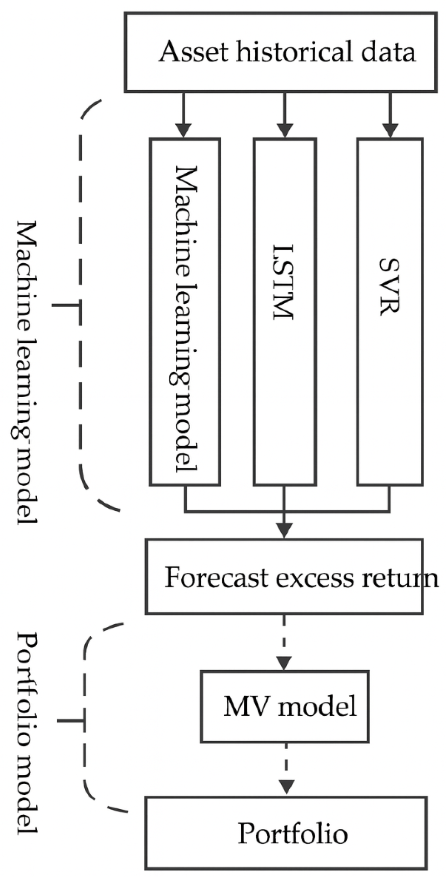
Figure 2.
Relationship Between Observable Data and Predicted Excess Returns.
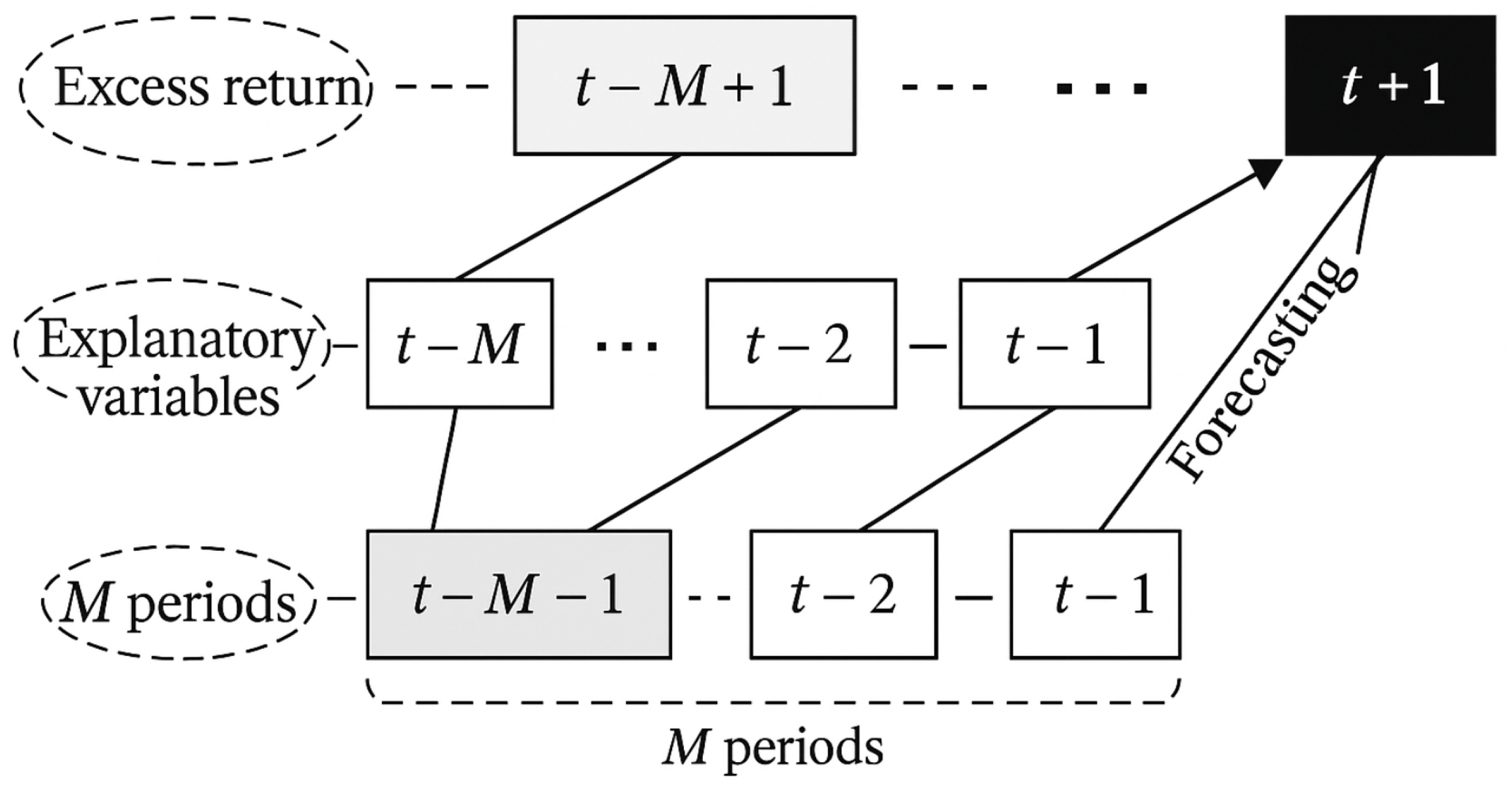
Figure 3.
Illustration of the Sliding Window Method.
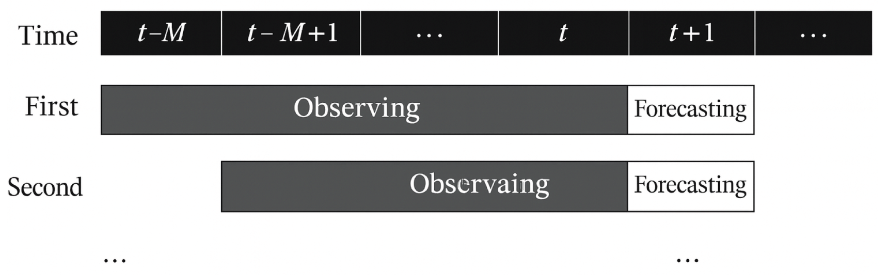
Figure 4.
Structure of the Transformer Model.
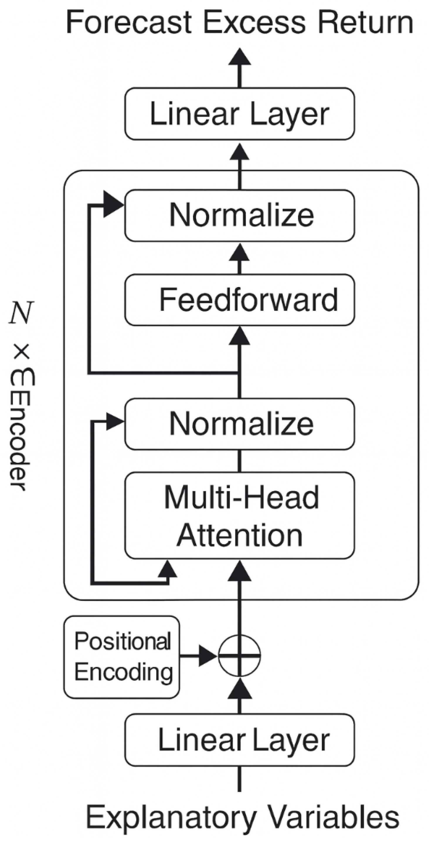
Figure 5.
Distribution of Selected Stocks by Shenwan First-Level Industry (December 2014).
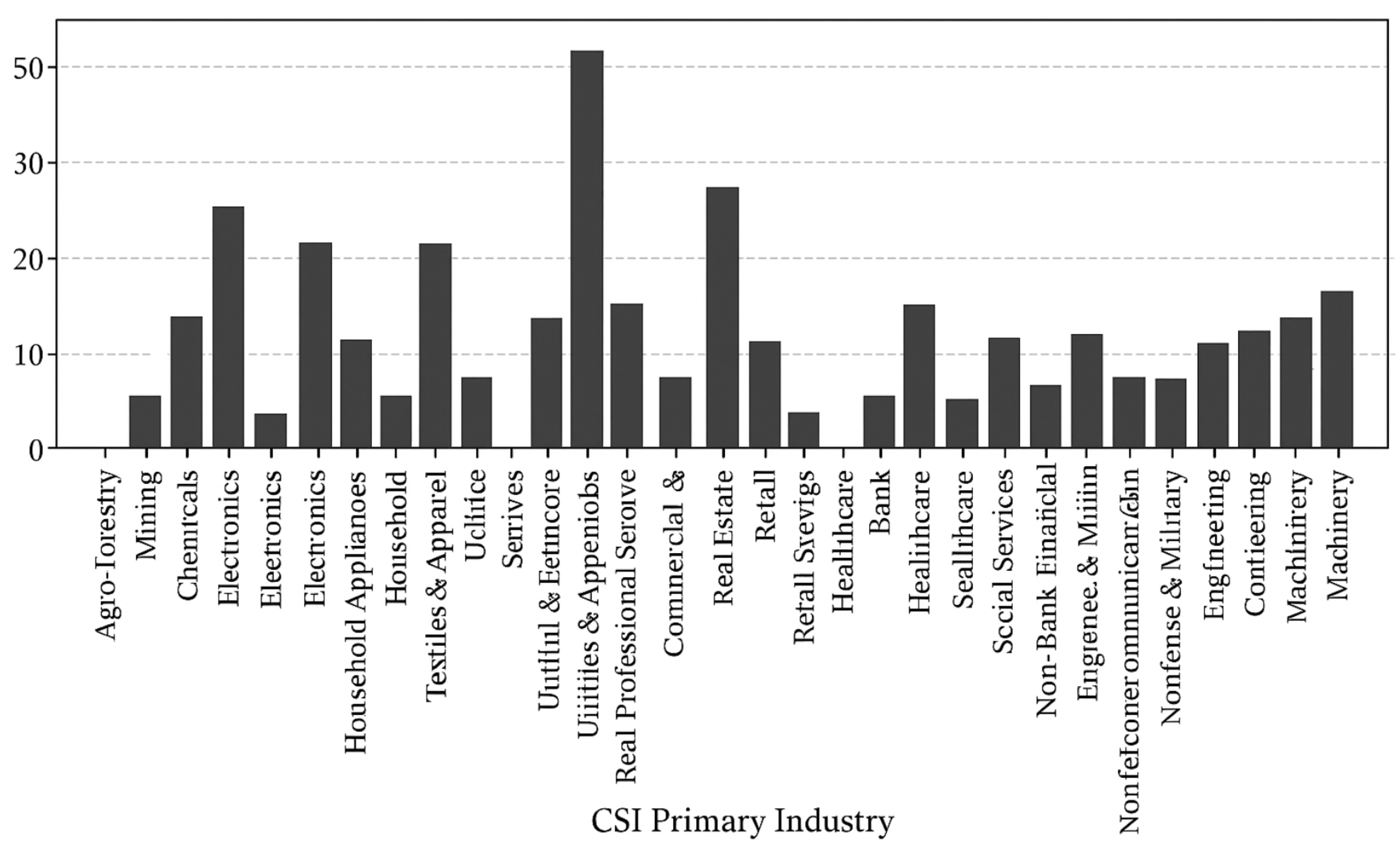
Figure 6.
Cumulative Returns of Portfolios Constructed Using the MV Model.
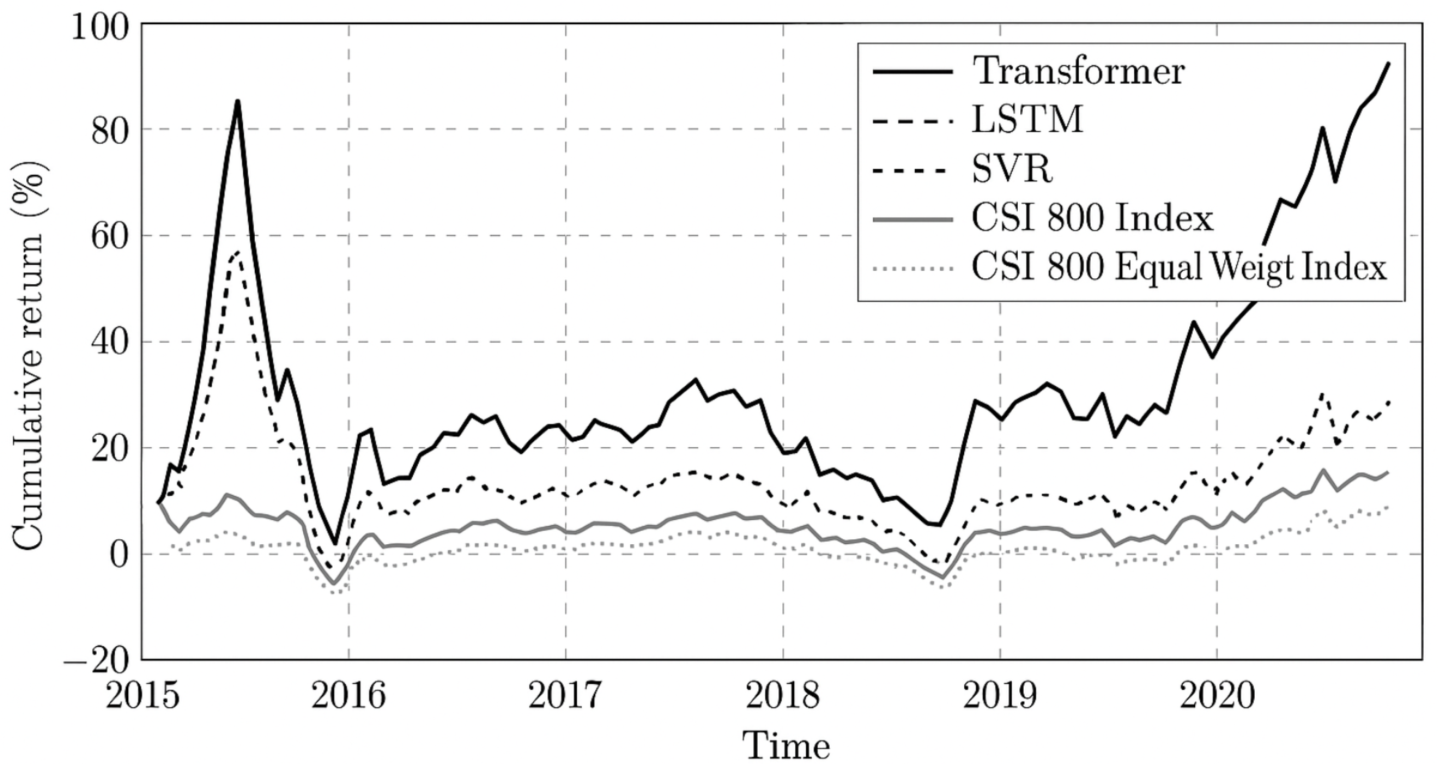
Table 1.
Explanatory Variables.
| Variable | Description |
|---|---|
| Industry | First-level industry classification (Shenwan) |
| ROE | Return on equity |
| E/P | Earnings-to-price ratio |
| Inflation | Inflation rate, CPI (YoY) |
| Rf | Risk-free rate, Shibor (1-month) |
| Turnover | Average daily turnover rate |
| Reversal | Reversal factor, excess return of current month |
| Size | Market capitalization |
| B/M | Book-to-market ratio |
| D/P | Dividend yield |
Table 2.
Descriptive Statistics of Explanatory Variables (June 2012 to December 2014).
| Variable | Unit | Mean | Std. Dev. | Min | Median | Max |
|---|---|---|---|---|---|---|
| ROE | % | 2.78 | 11.25 | -744.70 | 2.49 | 194.19 |
| E/P | 0.05 | 0.05 | -0.34 | 0.06 | 0.79 | |
| Inflation | % | 2.29 | 0.48 | -1.40 | 2.60 | 3.20 |
| Rf | % | 0.38 | 0.07 | 0.20 | 0.38 | 0.61 |
| Turnover | % | 1.45 | 1.44 | 0.02 | 1.06 | 26.24 |
| Reversal | % | 1.42 | 12.22 | -37.25 | 0.61 | 266.80 |
| Size | CNY 100M | 260 | 700 | 0.98 | 88 | 17000 |
| B/M | 0.47 | 0.30 | -0.12 | 0.48 | 2.47 | |
| D/P | % | 1.37 | 1.64 | 0.00 | 0.93 | 29.19 |
Table 3.
Hyperparameters of Prediction Models.
| Model | 2015–2017 | 2018–2020 |
|---|---|---|
| Transformer | d_model=288, nhead=6, dim_feedforward=288, n_layer=3, dropout=0.1 |
d_model=288, nhead=6, dim_feedforward=288, n_layer=3, dropout=0.1 |
| LSTM | hidden_size=192, n_layer=3 | hidden_size=256, n_layer=4 |
| SVR | kernel=rbf, gamma=0.001, C=0.01 | kernel=rbf, gamma=1, C=0.01 |
Table 4.
Comparison of Prediction Errors Across Models.
| RMSE | MAPE | |||||
|---|---|---|---|---|---|---|
| Model | Mean | Std | Skew | Mean | Std | Skew |
| Transformer | 0.124 | 0.056 | 1.754 | 610 | 1998 | 7.60 |
| LSTM | 0.132 | 0.052 | 1.329 | 1980 | 11991 | 8.28 |
| SVR | 0.115 | 0.050 | 1.572 | 1949 | 14346 | 8.30 |
Table 5.
Investment Performance of Portfolios Constructed Using the MV Model.
| 2015 | 2016 | 2017 | 2018 | 2019 | 2020 | Cumulative | Annualized | Sharpe | |
|---|---|---|---|---|---|---|---|---|---|
| Transformer | 20.76 | -9.95 | 12.51 | -19.02 | 39.21 | 50.78 | 107.96 | 12.98 | 0.46 |
| LSTM | 1.55 | -1.28 | -2.50 | -28.71 | 18.65 | 23.61 | 4.84 | 0.79 | -0.05 |
| SVR | 8.94 | -9.23 | 7.97 | -6.26 | 45.12 | 46.66 | 53.02 | 7.35 | 0.25 |
| CSI800 | 14.91 | -13.27 | 15.16 | -20.44 | 31.75 | 29.51 | 48.10 | 5.79 | 0.21 |
| CSI800 Equal | 36.90 | -15.07 | 0.44 | -31.31 | 27.44 | 19.32 | 21.99 | 3.77 | 0.11 |
Disclaimer/Publisher’s Note: The statements, opinions and data contained in all publications are solely those of the individual author(s) and contributor(s) and not of MDPI and/or the editor(s). MDPI and/or the editor(s) disclaim responsibility for any injury to people or property resulting from any ideas, methods, instructions or products referred to in the content. |
© 2025 by the authors. Licensee MDPI, Basel, Switzerland. This article is an open access article distributed under the terms and conditions of the Creative Commons Attribution (CC BY) license (http://creativecommons.org/licenses/by/4.0/).
Copyright: This open access article is published under a Creative Commons CC BY 4.0 license, which permit the free download, distribution, and reuse, provided that the author and preprint are cited in any reuse.


