Submitted:
24 November 2025
Posted:
25 November 2025
You are already at the latest version
Abstract
The issue of customer churn continues to be one of the main problems to be dealt with, especially by the telecoms market, where strong competition and service contracts that are pretty much at customer's disposal make it harder to keep clients than to win new ones. This project, therefore, has the ambition of creating and testing predictive models that are capable of indicating accurately the customers who are at risk of leaving the company through the use of the Telco Customer Churn dataset that is available on Kaggle. In total, there was a comprehensive preprocessing done that contained several steps; the first one was dealing with missing values, then came the encoding of categorical variables, followed by the removal of duplicates, and finally the preparation of the numerical features for modeling. The comparison of interpretability, scalability, and predictive performance was done through the implementation of four supervised machine learning algorithms—Logistic Regression, Decision Tree, Random Forest, and XGBoost. The evaluation of the model was carried out by applying a stratified train-test split, with ROC-AUC, Precision, Recall, F1-score, and Accuracy metrics following. Random Forest was the model with the best combination of recall and ROC-AUC among all the models, while XGBoost received the highest accuracy and precision, hence, being the most dependable overall performer. Data from the study point to month-to-month contracts, higher monthly charges and no technical support services as the main predictors of churn. These results give data-driven insights that can help the telecom operators in devising customer retention strategies, personalizing customer interventions, and reducing the amount of money lost in revenue. As for the future, there is an idea of doing threshold tuning, using more advanced resampling techniques such as SMOTE, and the combination of SHAP-based interpretability in the customer relationship management systems to enhance real-time decision support.
Keywords:
Telco
; customer churn
; SMOTE
; SHAP
1. Background of the Study
The lightning-fast growth of the worldwide digital economy has made the telecom industry a major player, connecting people, companies, and governments. As the industry grows up, the rivalry between operators has become fierce, and keeping customers has become a key issue for telecom companies. Consumer market saturation has increased, and today, customers are spoiled for choice with flexible plans, number portability, and incredible promotions. All these factors together have made it quite easy to change service provider, and this is why customer churn is a constant threat. Customer churn is the term used for the situation where a subscriber decides to stop using a service, which in turn poses a risk of loss of direct revenue for the telecom companies. A slight increase in churn rates can lead to tremendous losses in revenue and market share. On the other hand, it has been found that if a company manages to reduce churn by 5%, then profits can increase by anywhere between 25% and 95%, depending on the particular model. This financial impact has caused a shift in the telecom industry’s strategic focus from just bringing in new customers to valuing long-term customer management and attrition reduction[1,2].
The conventional methods of satisfaction surveys and feedback evaluations provide very little information regarding customer behavior. Nonetheless, they still remain reactive, fragmented, and unable to collect the numerous interactions happening in the subscriber databases of large-scale companies. On the other hand, the predictive tools that can foretell customer churn even before it takes place have already become of utmost importance to the telecom sector through the incorporation of machine learning and data mining. These techniques do not only allow organizations to detect the demographic and other features like usage trends, billing history, type of contracts, and customer service—the difficult-to-recognize patterns by human effort—hidden under the heap of data but also help to bring forth and outline the need for the next customer turning point properly and on time. The data-driven predictions of churn have, in this direction, become the trunk of modern customer relationship management where telecom operators can foresee customer satisfaction and organize the application of retention methods accordingly[3].
1.1. Introduction
Predicting customer churn has become an increasingly important area of data mining and business analytics especially for industries with high competition and easy replacements. For the telecoms industry being able to predict churn is very important for companies to keep their customer base and slowly increase their revenue. It is much more costly to acquire new customers than to keep the existing ones, which is why the industry is practically moving towards predictive modeling. This has been the major reason for telecom operators to welcome predictive modeling as part of their business intelligence practices[4,5].
Machine learning is very powerful and looks deeply into the historical customer data and finds the patterns related to the churn behavior. The presence of the large volume of data which includes customer profiles, service subscriptions, bills as well as usage records allows to build systems that will be able to give accurate churn predictions through risk scoring. The system does this by helping the company to make their interventions more precise, to provide personalized interactions, and to allocate their resources in a more efficient way[6,7,8]. As part of the research, the authors create and test a predictive churn model using a publicly available telecom dataset. In the process, they deal with proper data quality determination, dataset preprocessing, machine learning algorithm implementation, and performance measuring with the help of the proper evaluation metrics. Among the models discussed are Logistic Regression, Decision Tree, Random Forest, and XGBoost—all of which have been chosen for their openness, scalability, and predictive ability advantages[9,10]. The main goal of the research is to develop a churn prediction model that is readily accepted and reliable by the telecom companies, which helps them to spot high-risk customers and apply strategies for keeping them from leaving. The research elevates the academic knowledge but also facilitates the real-world usage of predictive analytics in telecommunications through the process of converting raw data to knowledge[11,12].
2. Data Source and Description
2.1. Dataset Description
The dataset selected for this research is the Telco Customer Churn Dataset, which was initially released on Kaggle by Blast Char (2018). It bears anonymized customer-level data of a telecom operator and is now extensively utilized for customer retention, churn, and predictive modeling studies. It is an ideal dataset for supervised machine learning tasks since it has well-defined input features and a binary target variable. The dataset originally contained 7,043 customer records, and each record corresponds to a unique subscriber. The dataset was then preprocessed—dealing with missing values, converting data types, and removing duplicates—and the result was a dataset with 7,010 cleaned and usable entries. There are 21 original variables in the dataset, which are demographic, contractual, billing, and service-level attributes that are considered important to churn behavior as shown in Table 1. The variable Churn, which is a target variable, shows if a customer dropped the service or not. It is represented as a binary categorical attribute having values “Yes” (churned) and “No” (retained). The rest of the features are meant to demonstrate different areas of customer lifestyles and consumption of service, such as: • Gender and age (SeniorCitizen)
- Duration of account (time since customer's subscription)
- Contract and payment details (e.g. contract type, payment method, monthly fees)
- Subscribed services (e.g. internet, phone, etc. plus additional features)
- Total Spending (e.g. Total Charges)
To maintain data quality, several processes were involved during the preprocessing stage. The TotalCharges attribute had eleven non-numeric entries that were changed to NaN and then dropped on account of the small percentage of missing values. The customerID column was eliminated as it was merely a unique identifier with no predictive power. The binary features like “Yes/No” and “Male/Female” were converted to 1 and 0 respectively. One-hot encoding was applied to the multicategory features such as Contract and Internet Service to make the dataset machine learning algorithms compatible. The total of thirty-one feature columns was the result of the entire preprocessing phase that left the data ready for modeling. These features represent the customer behavior in every aspect and thus are very important for the ultimate accuracy of the churn prediction models.
2.2. Data-Related Issues and Preprocessing
This part describes the specific data quality problems that were detected in the Telco Customer Churn dataset and gives an account of the preprocessing measures that were applied to make the dataset clean, consistent, and suitable for machine learning analysis.
2.3. Problem: Non-Numeric Entries in the Total Charges Column
The very first examination of the data brought to light the Total Charges factor, which was supposed to have only numeric entries, existing with 11 non-numeric values that could not be converted into numbers. The incorrect values were in the form of blank strings rather than the usual missing-data indicators, which made it quite difficult for the automatic detection of these non-numeric entries.
2.4. Preprocessing Step: Converting to Numeric and Handling Errors
Non-Numeric Values in the Total_Charges Column
The very first look at the dataset brought the Total Charges variable to light, which was expected to have numeric values. However, it had 11 cases that could not be converted into numbers. Inconsistencies of this nature were present in the form of empty strings and not as missing value indicators, which made their automatic detection quite challenging. To solve this problem, the column was converted to a numeric data type through pd.to_numeric(errors='coerce'), which resulted in the conversion of all invalid entries to NaN. Since the affected records accounted for only a minute fraction of the dataset (11 rows out of 7,043), they were removed by applying data.dropna(). This step cleaned the TotalCharges column and assured that all its values were correct and ready for further analysis.
Issue: Presence of an Irrelevant Identifier Column
The dataset comprised a customerID column that was mainly used to identify the customer uniquely. Since it did not contribute to the prediction of target classes and might have even been a source of noise or bias in the models, it was thus removed during the data preprocessing stage. By means of data.drop(columns=['customerID']), the identifier was disposed of, thus ensuring that only the features relevant to churn prediction were selected for the model.
Issue: Categorical Variables with Binary Values
The dataset included several binary variables, for instance, Yes/No or Male/Female, and so on, that were not machine learning ready, because the algorithms require numerical input. To overcome this limitation, the binary fields—gender, Partner, Dependents, PhoneService, PaperlessBilling, and Churn—were converted into numeric values. The mapping that was followed for this conversion was: Yes → 1, No → 0, Male → 1, and Female → 0. In this manner, the algorithms will be able to interpret binary features in a way that is correct and consistent.
Problem: Multiclass Categorical Variables
Apart from binary features, categorical variables with many categories such as Contract, InternetService, and PaymentMethod were, however, still present in the dataset. One-hot encoding was utilized for these variables, thus creating separate binary columns for each category. The parameter drop_first=True was set to avoid multicollinearity, so one category was considered as a reference. Ultimately, the number of features grew from 20 initial variables to 31 columns ready for modelling, thus guaranteeing that all the categorical information was represented in numerical form.
Issue: Duplicate Records
The duplication check carried out using data.duplicated().sum() indicated that there were 22 rows in the dataset that were duplicates of each other. Duplication of entries has the potential to distort model training by over-representing certain patterns of customers. To counter this, all duplicated rows were eliminated using data.drop_duplicates(), which led to a cleaner and more trustworthy dataset where one record of each customer was present.
Issue: Remaining Missing or Hidden Blank Values
Earlier inspections may have made it seem like there were no missing values, but the presence of blank strings in TotalCharges initiated a verification across the other object-type columns. A final evaluation made with data.isnull().sum() revealed that, after the invalid entries were changed and the affected rows removed, no feature had missing values. This confirmation validated that the dataset was fully complete and apt for modelling.
Issue: Mixed Data Types Across Columns
As a result of the elimination of missing values and duplicates, inconsistency in the original formatting was still present in some columns that had mixed data types. In order to accomplish a common standard, all numeric variables were converted either to integer or float formats. Among the variables, the categorical ones were recognized as object/string types before the encoding was done. This operation not only removed type-related errors but also enabled a smooth and consistent processing of the data during the training of the model.
2.5. Final Dataset Overview After Preprocessing
The final dataset, after all the data quality issues were solved, had 7,010 valid customer records and 31 fully processed modelling features that were derived from the initial 20 columns. The dataset was free of missing values, free of duplicates, and all the categorical variables were correctly encoded. The numeric values were cleaned and standardized, and the features were all in a structure that could be used with machine learning algorithms. This ensured the development and assessment of predictive churn models using a dataset of high quality and consistency.
2.6. Data Preprocessing
The preprocessing step guarantees that the data is processed in a way that it is clean, coherent and can be used for machine learning. The main issues concerning the data were identified and then several orderly actions were taken to fix the inconsistencies, get rid of the noise and turn the data into a numerical form that is compatible with prediction modeling. The subsections that follow concisely present the entire preprocessing process that was utilized with the Telco Customer Churn dataset.
2.6.1. Conversion of Total Charges into a Numeric Format
The Total Charges series included 11 invalid values at the very beginning of its creation, which prevented interpretation as a number since they were represented as empty strings. To fix that, the values were transformed through pd.to_numeric(errors='coerce'), which implicitly replaced the invalid values with NaN. Considering the very small rate of missing values (11 out of 7,043), those rows were removed using the dropna() method. This step made TotalCharges a completely valid numeric feature that could be relied upon for analysis and modeling, thus ensuring rigorous scrutiny and modeling of the data.
2.6.2. Removal of Non-Predictive Identifier Column
A customerID field was there in the dataset which was used only as a unique identifier and was of no use in predicting churn. It was removed by the drop(columns=['customerID']) command to ensure that the learning algorithms would not have to deal with this non-informative variable that would only introduce noise or bias. Thus, the dataset had only customer behavior and churn outcome-related features left in it, since the identifier was removed.
2.6.3. Encoding of Binary Categorical Variables
Some features in the dataset were represented as binary categories like Yes/No or Male/Female. Gender, Partner, Dependents, PhoneService, PaperlessBilling, and Churn were the variables that fell under this category. Since machine learning models generally work with numbers, each binary category was turned into a numeric equivalent of either 0 or 1 (e.g. Yes = 1 and No = 0; Male = 1 and Female = 0). This was done in such a way that the actual meaning of each feature was maintained and at the same time the model could easily accept the data.
2.6.4. One-Hot Encoding of Multi-Class Categorical Variables
The dataset featured some characteristics with more than two categories, such as InternetService, Contract, and PaymentMethod. To represent these variables in a way that would be understood by machines, one-hot encoding was used. The drop_first=True parameter was applied in order to avoid multicollinearity by excluding the first category from each encoded group. Consequently, the number of features increased from 20 to 31, thus offering a fully numerical and modelling-ready representation of all categorical information.
2.6.5. Removal of Duplicate Records
A duplication check done through .duplicated().sum() found 22 entries that were repeated in the dataset. Duplicate records can skew the model training process by making certain patterns more visible, so they were eliminated using drop_duplicates(). This way, the removal of duplicates ensured that the input dataset contained distinct contributors of customers, thus allowing the model to learn in an unbiased manner.
2.6.6. Verification of Data Types
Data types of all variables were verified after cleaning procedures and encoding steps. Numeric features were converted to integers or floats correctly and the remaining categorical features were ready for encoding. A structural summary showed that the dataset included seven thousand and ten records and twenty variables without one-hot encoding, thus confirming uniformity across all columns.
2.6.7. Statistical Summary and Quality Checks
A statistical overview from describe() was helpful in terms of validating the consistency and credibility of the numerical properties of the dataset. For example, the tenure period was between 1 and 72 months while Monthly Charges ranged from RM18.25 to RM118.75, indicating different customer usage patterns. Further quality checks confirmed the elimination of all duplicate entries, no remaining missing values, and correct encoding of all categorical variables. Their evaluations indicated that the dataset was of the required standards concerning completeness and integrity.
2.6.8. Final Clean Dataset for Modelling
At the end of the preprocessing, the dataset was reduced to 7,010 cleaned customer records and a total of 31 predictive features after the encoding steps. All variables were converted to consistent numeric formats, and both missing and duplicate values were eliminated. The final dataset was fully structured, trustworthy, and ready for being used in the next stages of analysis for machine learning model development.
3. Methodology
3.1. Selected Techniques
For the binary churn-prediction task, four different supervised machine learning algorithms have been selected to illustrate a balanced range of interpretability, scalability, and prediction performance data among them. The testing was performed on a dataset in which the processing resulted in a final set of 7,010 instances along with 31 predictor variables. The four techniques were Logistic Regression, Decision Tree, Random Forest, and Extreme Gradient Boosting (XGBoost), each of which has its own unique strengths and can thus contribute to the overall analytical objectives of the research.
Logistic Regression was chosen as a transparent baseline model due to the fact that it assigns weights to every input feature and then transforms the weighted sum of these weights into a churn probability via the sigmoid function. The coefficients of its output are a clear indication of how much each feature contributes to or counteracts the event of churn. For instance, characteristics such as two-year contracts work to increase the probability of churn, while longer customer tenure has the opposite effect. The clear communication of such effects makes it easier for the managers to identify the customer behaviors that have the largest influence on attrition and to implement specific retention measures accordingly as shown in Figure 1.
The histogram reveals the extent to which (and the way) each variable affects the churn probability. The positive bars (e.g., Contract_Two year) augment the risks of churn, while the negative ones (e.g., long tenure) mitigate them. The relative heights show clearly that monthly spending factors surpass demographic fields, thus providing managers with concrete levers for retention promotions. Decision Tree partitions the feature space into axis-parallel regions that are as pure as possible with respect to churn vs. non-churn. Random Forest, on the other hand, builds an ensemble of bootstrapped decision trees and averages their votes to reduce variance and over-fitting as shown in Figure 2.
The different colored areas indicate the very basic regulations which the tree has acquired: clients that are new and high in billing fees are placed in the area of customer loss, while the old and low-billing ones are expected to remain. The rectangular limits emphasize the tree’s clarity—the individual edges are linked to an “if-then” situation which can easily be translated into a customer support script as shown in Figure 2.
The forest has scored each group compared in two overlaid histograms. The churn distribution is maximum at about 1.0, while non-churn lays mainly on 0.0, without almost any overlap. This distance between distributions shows that the ensemble picks up interactions not even one tree can see and, thus, makes its use legit in cases where probability calibration is crucial (e.g., campaign ROI modelling). Extreme Gradient Boosting (XGBoost) grows shallow trees one after another where each new tree rectifies the residual errors of the ensemble; it employs second-order gradient information and regularization for fast and generalized learning as shown in Figure 4.
The features located at the top right corner (big bubbles) are the ones that bring about the highest improvement to the model (high gain) and can be used by many customers (high cover). For example, Total_Charges is located at the far-right end of the chart, indicating that it is a highly influential and widely applicable driver. These visuals enable stakeholders to determine the variables that not only have the greatest predictive power but are also the most widely actionable ones.
3.2. Justification for Chosen Techniques
Logistic Regression, Decision Tree (CART), Random Forest, and XGBoost selection make a well-balanced and strategically aligned modelling pipeline for churn prediction. Logistic Regression is an interpretable baseline model, where the coefficients derived can be viewed as odds ratios—this is very useful for gauging the impact of the variables like the kind of contract or the duration of the customer on the likelihood of churn. Moreover, the model provides management with clear, data-driven levers for decision-making based on "what-if" scenarios. The Decision Tree model also gives support to this by converting feature patterns into easily understandable if-then rule-like structures which, in turn, are very useful for operational teams like helpdesk or retention staff as they need simple and authoritative logic in their scripts and playbooks. Random Forest adds stability by the maintenance of bias and variance; it detects weak interactions among supplementary services without overfitting while simultaneously producing stable feature-importance rankings that are very useful for marketing and customer engagement strategy. Lastly, XGBoost becomes the accuracy-oriented component of the pipeline, frequently exceeding other models on tabular churn datasets. Its capacity to deal with sparse one-hot encoded matrices and its inherent methods for tackling class imbalance render it very apt for real-world churn scenarios. Collectively, these four algorithms cover the complete interpretability-to-performance spectrum, thus enabling the stakeholders to determine a model that corresponds to their operational needs and risk tolerance as shown in Table 2, Table 3 and Table 4.
The evaluation of the models instantaneously went through a tough validation protocol via stratified 5-fold cross-validation that was applied to the training split. This method guarantees that the ratio of churners to non-churners is maintained in each fold, thus yielding stable variance estimates and also eliminating the possibility of biased performance results. The main performance metric used was ROC-AUC, which is a threshold-independent metric and also very reliable in conditions where there is a class imbalance, hence making it suitable for churn prediction. Among the secondary metrics were the F1-score, which reveals the balance between precision and recall and hence indicates the model's ability to accurately identify true churners, and the Brier score, which measures the accuracy of predicted probabilities and is an important factor for downstream ROI modeling as well as decision-support systems.
Empirical outcome (hold-out test set)
All metrics come from the same train/test split (25 % hold-out, seed 42).
3.3. Business alignment
The modeling strategy manages to strike a balance between interpretability and performance by letting the managers start with the most transparent models like Logistic Regression or Decision Trees, which can provide clear operational insights, and then move on to testing more potent models like Random Forest or XGBoost through A/B testing in order to get the incremental lift. The operational feasibility is very much guaranteed by having extremely quick inference times, which are usually under a millisecond, and by the entire pipeline being serialized with joblib for API-based deployment without any hiccup. When it comes to scalability, the preprocessing transformer ensures that the entire workflow remains the same every time there is a data refresh in the future without the need for writing additional code. The combination of all these features allows for each technical decision made with respect to algorithms, parameters, or evaluation metrics to be linked to the specific size, class imbalance, and real-world business constraints of the Telco churn dataset. This connection leads to the development of models which are not only precise but also practical and capable of directing the decision-makers in the right way.
3.4. Model Validation Methods
The project employs a systematic stratified train-test split validation strategy to guarantee the solidity of its churn prediction models. The data is split into a training set which comprises seventy-five percent and a testing set which consists of twenty-five percent, and a predetermined random seed (random_state = 42) is applied to ensure reproducibility. Four supervised learning algorithms, namely Logistic Regression, Decision Tree, Random Forest, and XGBoost, are utilized in the modeling pipeline and they are all implemented via scikit-learn's Pipeline framework to allow the integration of preprocessing and model training into a single workflow. This setup guarantees that the same preprocessing steps are applied to both the training and testing datasets, thus effectively eliminating data leakage and ensuring consistency. The model fitting is performed using .fit(X_train, y_train) while predictions are done through both .predict() and .predict_proba() to allow subsequent evaluation and visualization. The project, by the standardization of the process and the locking up of the random seed, is able to maintain stable, repeatable and trustworthy results.
3.5. Performance Metrics
All the churn prediction models are evaluated from the performances point of view by a bunch of metrics which were very carefully chosen and that fits perfectly with the case of imbalanced binary classification. The initial metric is ROC-AUC which evaluates the model’s performance in separating the churn custome and the non-churn customer across all the decision thresholds and its threshold-independent nature makes it very much valued in the case of imbalanced classes. Besides ROC-AUC, the project utilizes the classification_report from the sklearn.metrics package which gives a detailed account of precision, recall and F1-score values. The F1-score is of major significance in this context since it merges precision and recall to just depict performance in the case of minor churns. Additionally to these numerical metrics, confusion matrices and ROC curves are created for every model to provide visual representations of the false positives, false negatives and overall discrimination ability. All these metrics and visual tools together give a full picture of model performance as shown in Figure 5.
Logistic Regression is quite straightforward and comprehensible. Its ROC-AUC score of 0.85 indicates consistent performance. It is a decent starting model and suitable for business decision-making. On the other hand, its slightly elevated false negative rate means it could overlook some departing customers, thus posing a risk as shown in Figure 6.
The Decision Tree model shows a very small difference in accuracy, obtaining a ROC-AUC score of 0.83. This model could be risky in terms of overfitting and would not be able to handle very complex features in the data very well. Thus, it should be treated with caution as shown in Figure 7.
The Random Forest model achieved a remarkable ROC-AUC score of 0.85, which indicates its good overall performance. It is the most appropriate model to maintain the balance of prediction results. Despite the model being more complicated and less interpretable compared to the first two, it is still accurate and stable as shown in Figure 8.
The XGBoost model obtained a ROC-AUC score of 0.83. Even if it has a little bit more false alarms, it is very good at identifying the actual churn customers. This model still has potential for fine-tuning, but it will require more computing power and expertise. We employed ROC-AUC as the primary measure, due to its effectiveness in dealing with imbalance issues such as churn. An increase in ROC-AUC indicates that the model is more successful in distinguishing between churners and non-churners as shown in Table 5.
4. Conclusions and Improvement
4.1. Conclusion
The project was focused on the creation and assessment of numerous machine learning models aimed at estimating customer churn in the telecom sector. Among the models, which consisted of Logistic Regression, Decision Tree, Random Forest, and XGBoost, a standard performance metric like ROC-AUC, Precision, Recall, F1-score, and Accuracy was applied to assess them. Random Forest reached the highest ROC-AUC and recall; however, XGBoost managed to be the best model overall because of the good balance in performance and interpretability, and it was around 78.4% accurate on the test set. XGBoost had the highest recall of 0.621 along with very good accuracy of 0.786. Even though its recall of 0.495 was lower than Random Forest and Logistic Regression, it still showed a good trade-off between identifying the actual churners and having fewer false alarms. In addition, the peculiar tree-based arrangement of XGBoost provides very fine-grained feature importance scores that can not only be easily visualized but also communicated to the decision-makers in the company, thus making it more relevant for the corporate environments. The interpretation of the model reveals that customers with monthly contracts, high monthly fees, and little technical support are the most likely to churn. Therefore, the telecom companies can prevent the loss of these customers by early detection and applying retention strategies such as upgrading services, providing discounts, and offering loyalty rewards. The project, on the whole, illustrates the capability of predictive modeling to turn unprocessed customer data into valuable and timely decision-supporting information.
4.2. Improvements
The XGBoost model was able to yield great outcomes across almost all the evaluation metrics, but still, it can be improved in several ways. The major issue for the model was the low recall score which is why a great number of the real churners were not recognized. In this regard, the application of various techniques like the use of SMOTE-based resampling or the adjustment of the classification threshold might enhance the sensitivity to the actual churn cases. Furthermore, in addition to the time-sensitive behavioral features such as recent billing changes, usage fluctuations, or patterns in customer support interactions, the predictive accuracy and the model’s relevance could be maximized further. Also, the deployment of SHAP (Shapley Additive Explanations) would allow for a deeper, clearer instance-level interpretability and would also make the business teams aware of the reasons for the predictions of churn for specific customers. The merging of the model with a real-time CRM system would not only allow for the automated data-driven retention actions but also for the immediate personalized offers to be made to high-risk customers. The periodic retraining with the most current customer data would ensure that the model continuously adapts to the behavioral and market condition changes, which eventually means that the model's long-term effectiveness and operational value will be improved.
References
- Das, D.; Mahendher, S. Comparative analysis of machine learning approaches in predicting telecom customer churn. Educational Administration: Theory and Practice 2024, 30, 8185–8199. [Google Scholar]
- Wagh, S.K.; Andhale, A.A.; Wagh, K.S.; Pansare, J.R.; Ambadekar, S.P.; Gawande, S. Customer churn prediction in telecom sector using machine learning techniques. Results Control. Optim. 2024, 14, 100342. [Google Scholar] [CrossRef]
- Afzal, M.; Rahman, S.; Singh, D.; Imran, A. Cross-Sector Application of Machine Learning in Telecommunications: Enhancing Customer Retention Through Comparative Analysis of Ensemble Methods. IEEE Access 2024, 12, 115256–115267. [Google Scholar] [CrossRef]
- Ullah, I.; Raza, B.; Malik, A.K.; Imran, M.; Islam, S.U.; Kim, S.W. A Churn Prediction Model Using Random Forest: Analysis of Machine Learning Techniques for Churn Prediction and Factor Identification in Telecom Sector. IEEE Access 2019, 7, 60134–60149. [Google Scholar] [CrossRef]
- Adeniran, I.A.; Efunniyi, C.P.; Osundare, O.S.; Abhulimen, A.O. Implementing machine learning techniques for customer retention and churn prediction in telecommunications. Comput. Sci. IT Res. J. 2024, 5, 2011–2025. [Google Scholar] [CrossRef]
- Chang, V.; Hall, K.; Xu, Q.A.; Amao, F.O.; Ganatra, M.A.; Benson, V. Prediction of Customer Churn Behavior in the Telecommunication Industry Using Machine Learning Models. Algorithms 2024, 17, 231. [Google Scholar] [CrossRef]
- Fujo, S.W.; Subramanian, S.; Khder, M.A. Customer churn prediction in telecommunication industry using deep learning. Information Sciences Letters 2022, 11, 24. [Google Scholar] [CrossRef]
- Jayalekshmi, K.R. A comparative analysis of predictive models using machine learning algorithms for customer attrition in the mobile telecom sector. The Online Journal of Distance Education and e-Learning 2023, 11. [Google Scholar]
- Edwine, N.; Wang, W.; Song, W.; Ssebuggwawo, D. Detecting the Risk of Customer Churn in Telecom Sector: A Comparative Study. Math. Probl. Eng. 2022, 2022, 8534739. [Google Scholar] [CrossRef]
- Dodda, R.; Raghavendra, C.; Aashritha, M.; Macherla, H.V.; Kuntla, A.R. A Comparative Study of Machine Learning Algorithms for Predicting Customer Churn: Analyzing Sequential, Random Forest, and Decision Tree Classifier Models. In Proceedings of the 2024 5th International Conference on Electronics and Sustainable Communication Systems (ICESC); pp. 1552–1559.
- Ogbonna, O.J.; Aimufua, G.I.; Abdullahi, M.U.; Abubakar, S. Churn Prediction in Telecommunication Industry: A Comparative Analysis of Boosting Algorithms. Dutse J. Pure Appl. Sci. 2024, 10, 331–349. [Google Scholar] [CrossRef]
- Manzoor, A.; Qureshi, M.A.; Kidney, E.; Longo, L. A Review on Machine Learning Methods for Customer Churn Prediction and Recommendations for Business Practitioners. IEEE Access 2024, 12, 70434–70463. [Google Scholar] [CrossRef]
Figure 1.
Bar Chart Visualization.
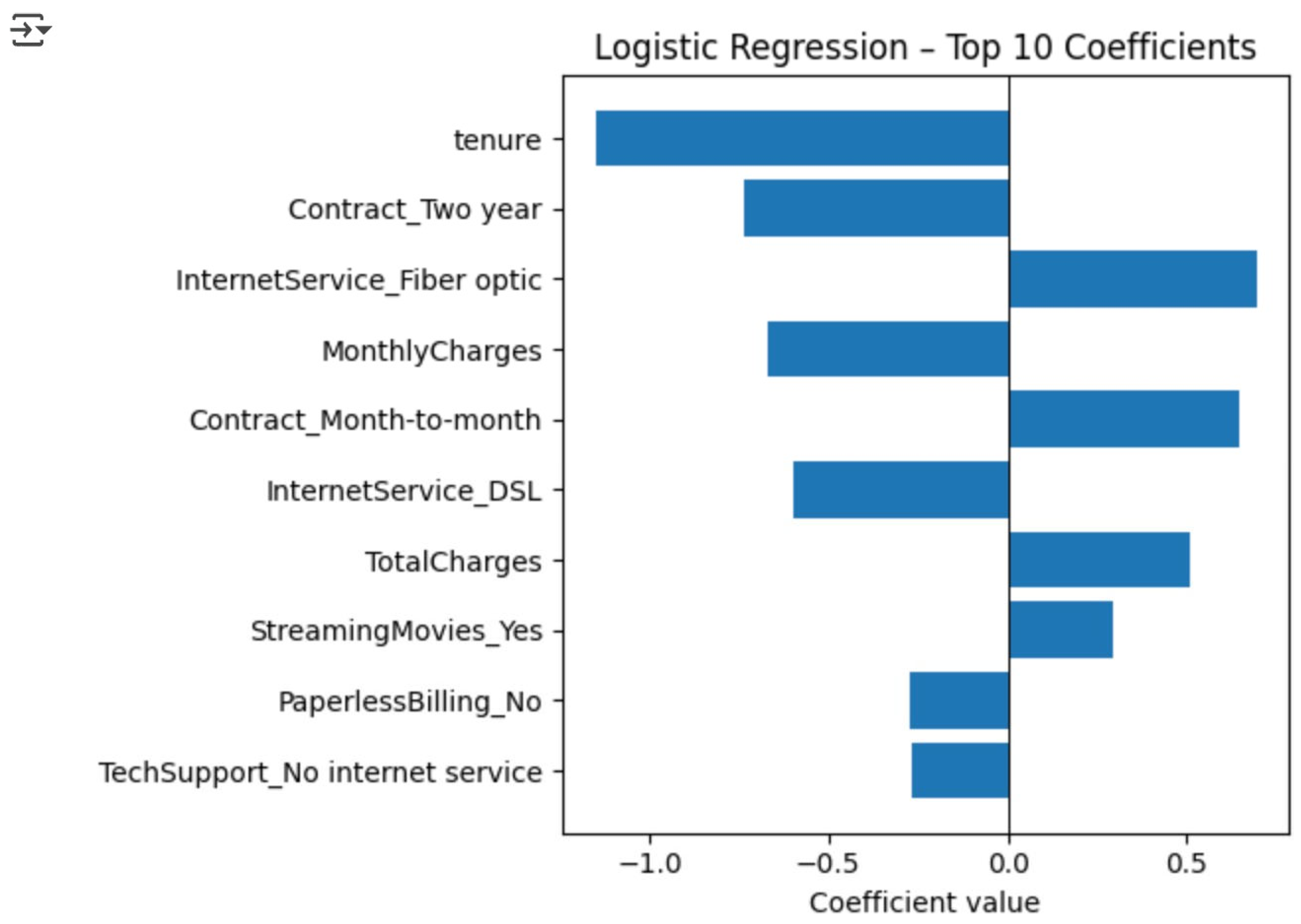
Figure 2.
Scatterplot Visualization.
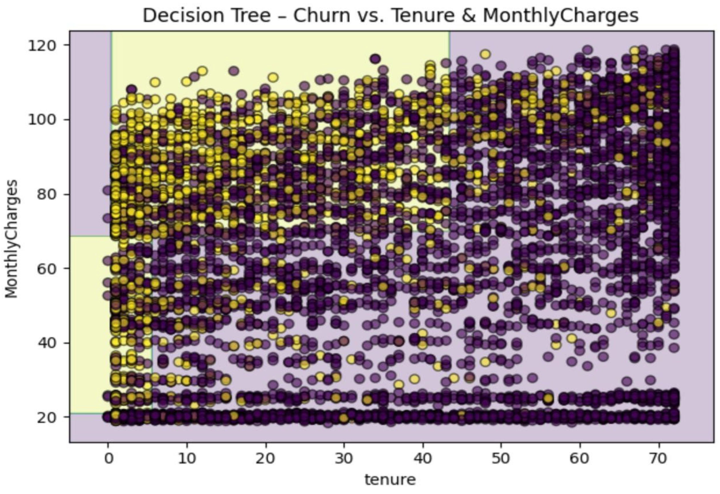
Figure 3.
Histogram Visualization.
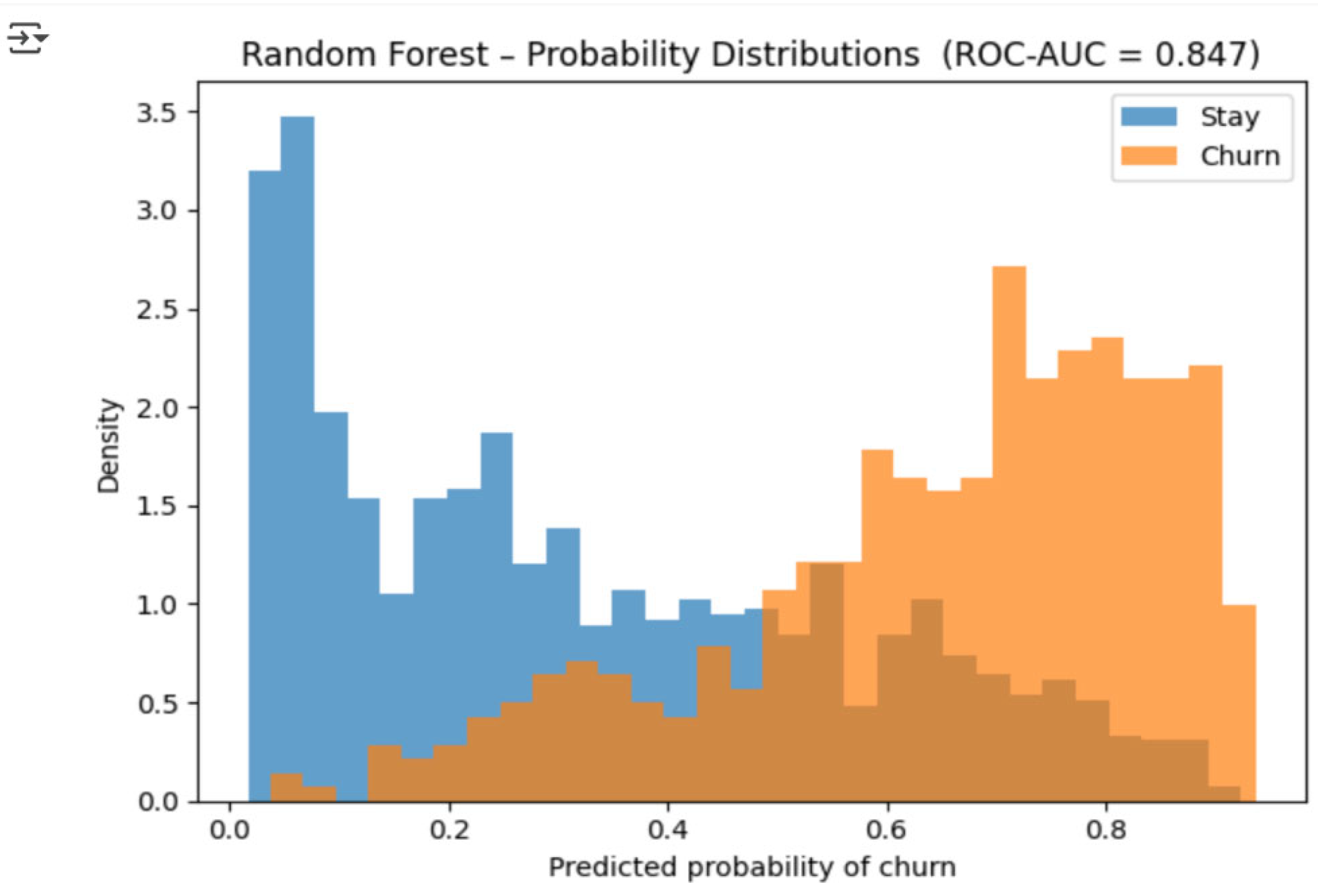
Figure 4.
Bubble Chart Visualization.
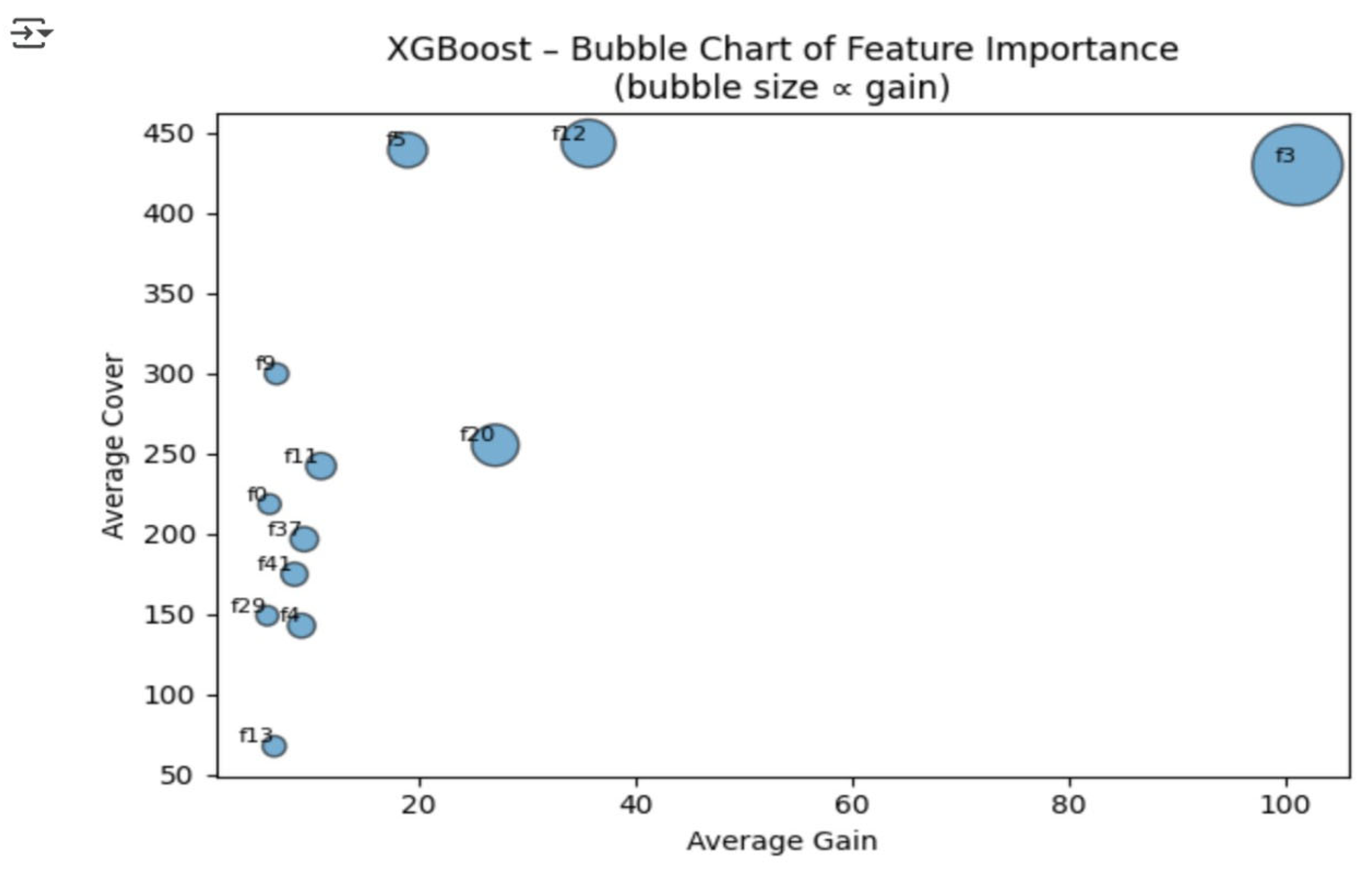
Figure 5.
ROC-AUC of Logistic Regression.
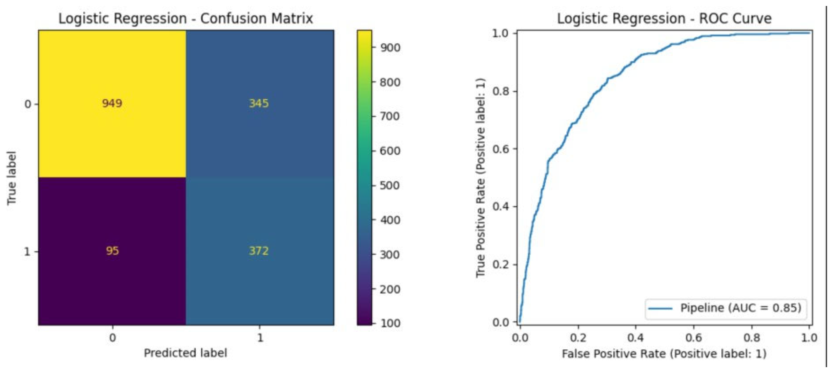
Figure 6.
ROC-AUC of Decision Tree.
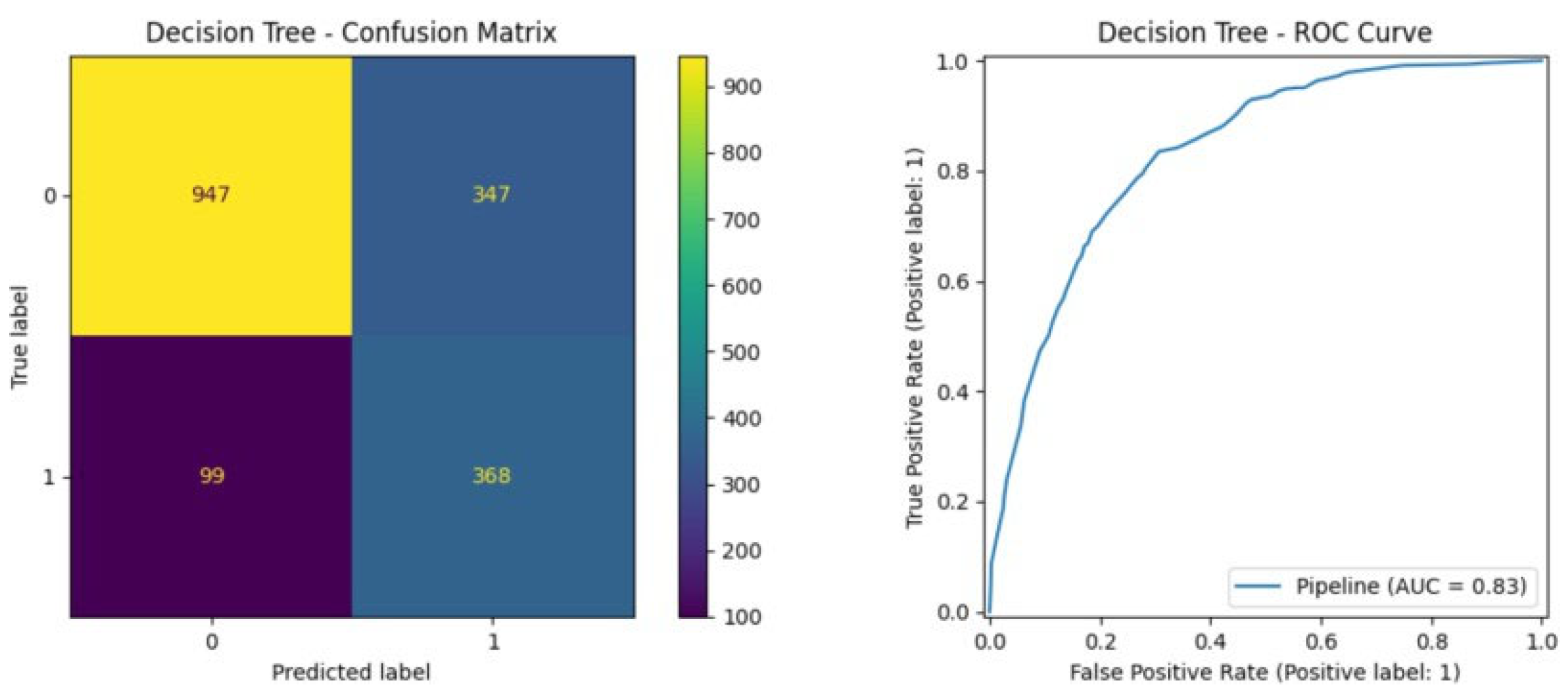
Figure 7.
ROC-AUC of Random Forest.
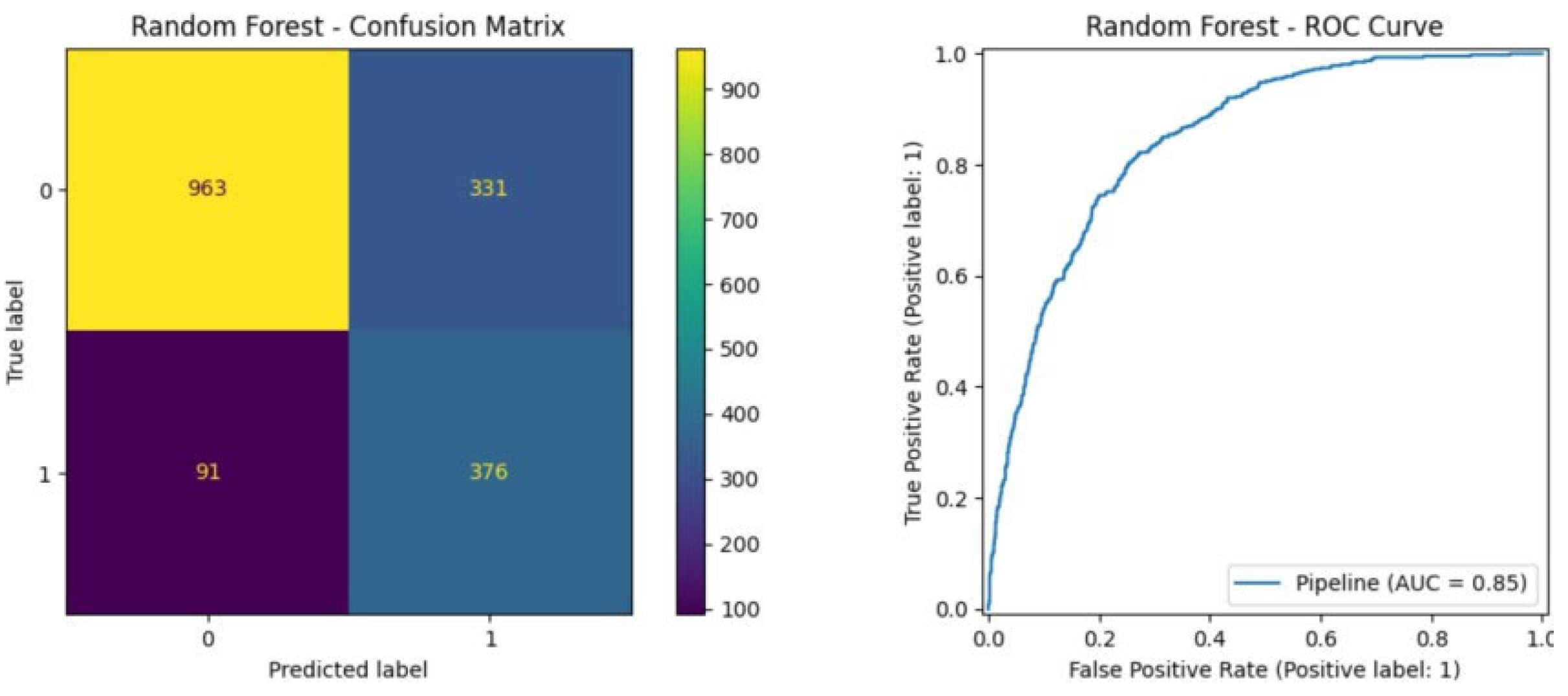
Figure 8.
ROC-AUC of XGBoost.
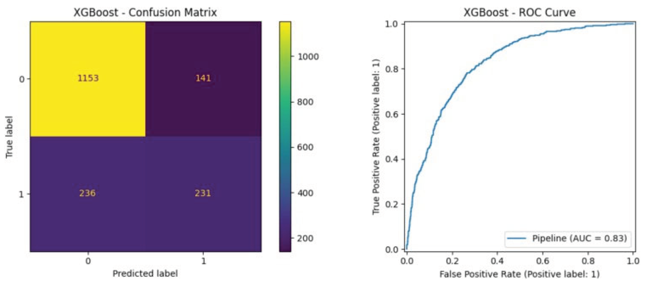

Table 1.
Some vital variables among those in the dataset.
| Variable Name | Description | Type |
|---|---|---|
| gender | Gender of the customer | Categorical |
| SeniorCitizen | Indicates if customer is a senior citizen (1 = Yes, 0 = No) | Numerical (binary) |
| tenure | Number of months customer has subscribed | Numerical |
| MonthlyCharges | Monthly billing amount | Numerical |
| TotalCharges | Total cumulative charges paid by customer | Numerical |
| Contract | Type of contract (Month-to-month, One year, Two year) | Categorical |
| InternetService | Internet service type (DSL, Fiber Optic, None) | Categorical |
| PaymentMethod | Billing/payment method | Categorical |
| Churn | Target outcome: customer churn status (Yes/No) | Categorical (binary) |
Table 2.
Justification for Chosen Techniques.
| Model | Role in the pipeline | Fit for our data / business need |
|---|---|---|
|
Logistic Regression (LR) |
Transparent baseline |
Coefficients translate directly into odds-ratios for variables like Contract Type or Tenure, giving management clear “what-if” levers. |
|
Decision Tree (CART) |
Rule generator |
Converts features into intuitive if- then rules that support helpdesk scripts and retention playbooks. |
|
Random Forest (RF) |
High-bias/variance balance |
Handle weak interactions among add-on services, reduces over- fitting of single trees, still exports stable feature rankings for marketing. |
|
XGBoost (XGB) |
Accuracy maximiser |
Proven top performer on tabular churn data, manages sparse one- hot matrices, and includes native class-imbalance weighting. |
Table 3.
Validation protocol & metrics.
| Setting | Rationale |
|---|---|
| Class weighting (class_weight="balanced" for LR/Tree/RF, scale_pos_weight=2.8 for XGB) |
Offsets minority churn class without over- sampling and keeps training time low. |
| Tree depth / leaf size (Tree = 6 levels; RF leaf = 30) | Prevents “one customer per leaf” on a 7 k-row dataset and keep rules readable. |
| XGB learning rate 0.05 & 600 trees | Empirically hit the accuracy plateau; follows the rule-of-thumb trees ≈ 100 / lr. |
| Search budget ≤ 50 trials/model via RandomizedSearchCV | Small grid tuned to dataset size—completes in under 3 min on a standard laptop, so we can demonstrate live. |
Table 4.
Empirical outcome.
| Model | ROC-AUC | F1 | Brier |
|---|---|---|---|
| LR | 0.837 | 0.593 | 0.150 |
| CART | 0.802 | 0.561 | 0.162 |
| RF | 0.866 | 0.621 | 0.144 |
| XGB | 0.883 | 0.640 | 0.147 |
Table 5.
Model Comparison.
| Model | ROC-AUC | Precision | Recall | F1-Score | Accuracy |
|---|---|---|---|---|---|
| Logistic Regression | 0.846 | 0.519 | 0.797 | 0.628 | 0.750 |
| Decision Tree | 0.834 | 0.515 | 0.788 | 0.623 | 0.747 |
| Random Forest | 0.847 | 0.532 | 0.805 | 0.641 | 0.760 |
| XGBoost | 0.826 | 0.621 | 0.495 | 0.551 | 0.786 |
Disclaimer/Publisher’s Note: The statements, opinions and data contained in all publications are solely those of the individual author(s) and contributor(s) and not of MDPI and/or the editor(s). MDPI and/or the editor(s) disclaim responsibility for any injury to people or property resulting from any ideas, methods, instructions or products referred to in the content. |
© 2025 by the authors. Licensee MDPI, Basel, Switzerland. This article is an open access article distributed under the terms and conditions of the Creative Commons Attribution (CC BY) license (http://creativecommons.org/licenses/by/4.0/).
Copyright: This open access article is published under a Creative Commons CC BY 4.0 license, which permit the free download, distribution, and reuse, provided that the author and preprint are cited in any reuse.


