1. Introduction
Rice serves as the primary food source for over half of the world's population [
1,
2], serving as a vital food crop for achieving the United Nations' Sustainable Development Goal 2030 of Zero Hunger [
3]. China ranks second globally in rice cultivation area, with a perennial planting area of 30 million hectares [
4]. In mechanized rice cultivation, the paddy field bottom layer serves as a critical component within the tillage soil structure, bearing the operational loads of agricultural machinery. During operation, machinery encounters vibrations, bouncing, and bogging due to uneven pits and ruts in the bottom layer, significantly impacting both the passage of machinery and the quality of field operations [
5,
6]. As agricultural production rapidly advances toward intelligent and labor-saving practices, the autonomous navigation and precise control capabilities of paddy field machinery have become critical for realizing smart farms with reduced labor requirements in rice production [
7]. However, the complex and variable contour of paddy field hard bottom layer surfaces [
8] remains poorly understood in terms of its impact on the position and attitude changes of agricultural machinery. This lack of clarity constrains the optimization of operation control strategies and hinders the advancement of intelligent operation levels. [
9,
10], it is imperative to elucidate the influence patterns of typical hard bottom layer contours on the position and attitude changes of agricultural machinery. Early terrain mechanics theories provided the foundation for modeling wheel-ground interactions. Bekker and Wong systematically established mathematical models for soft soil bearing capacity, settlement, and rolling resistance, offering theoretical support for vehicle dynamics response research. [
11,
12]. Jia et al. proposed a wheel-terrain interaction model based on wheel dynamics and terrain mechanics, effectively simulating wheeled movement in soft soil and enabling numerical simulations for off-road mobile robots [
13]. Misaghi et al. employed the International Roughness Index (IRI) to model road surface irregularities in truck-road interactions, quantifying the effects of truck suspension systems and road conditions on pavement damage [
14]. Zheng et al. identified the driving environment as the most significant external factor influencing vehicle dynamics. They investigated the effects of varying road roughness, adhesion coefficients, and road gradients on the dynamic performance of dual-clutch transmission vehicles [
15]. Inotsume and Kubota proposed an adaptive terrain passability prediction method based on multi-source transfer Gaussian process regression. This approach utilizes limited data from low-risk terrain within the target environment, combined with prior travel experience across diverse terrain surfaces [
16]. Golanbari identified soil deformation as a key factor affecting off-road vehicle performance. They investigated soil deformation caused by the interaction between pneumatic tires and track wheels with the ground. The fitted surfaces obtained using optimization algorithms effectively predicted soil deformation induced by different wheel types [
17].
In studies examining the impact of complex farmland topography on agricultural machinery operations, Tu et al. proposed methods for quantifying paddy field hard bottom layer contours, tillage layer thickness, and their characteristics based on machinery pose information. They developed a method for quantifying hard bottom layer contour features, providing a driving environment map for agricultural machinery [
8,
18,
19]. The primary factor affecting autonomous agricultural machinery path tracking accuracy is lateral deviation caused by skidding under terrain influence [
20,
21]. To address terrain-induced lateral deviation in agricultural machinery, Bevly, Ryu, and Anderson et al. employed a dual-antenna Global Navigation Satellite System (GNSS) system and Inertial Navigation System (INS) sensors to establish a kinematic model-based heading Kalman filter. This approach enabled the estimation of center-of-mass lateral deviation angles and front-rear wheel lateral deviation angles, further facilitating the estimation of wheel lateral deviation stiffness [
22,
23,
24]. To suppress disturbances from wheel lateral deviation, researchers treated lateral deviation as a disturbance term in linear motion models and employed robust control techniques for mitigation [
25]. Alternatively, they developed vehicle dynamics and kinematic models incorporating lateral deviation parameters, applying nonlinear control techniques to design path-tracking control laws [
26,
27]. Lenain et al. developed front and rear wheel yaw angle observers based on extended kinematic equations for front-wheel steering and four-wheel steering agricultural vehicles, utilizing dual-antenna GNSS and INS. They applied the estimated values to path tracking control, effectively enhancing tracking accuracy [
28]. Regarding operational effectiveness, Zhou et al. addressed the tilting and height fluctuations of leveling machines caused by uneven hardpan layers in rice fields. They designed a leveling machine based on dual-antenna GNSS positioning and orientation, achieving horizontal and elevation control of the leveling blade after terrain-induced attitude changes [
29]. He Jing et al. proposed a real-time terrain-aware dynamic adjustment method for rice row detection by integrating 2D LiDAR, Attitude and Heading Reference System (AHRS), and Real-Time Kinematic Global Navigation Satellite System (RTK-GNSS) data fusion [30].
The above research demonstrates that terrain undulations significantly impact vehicle driving stability and agricultural machinery operation quality. Relevant studies have laid a solid foundation for analyzing the operational characteristics of agricultural machinery in complex terrain conditions, covering aspects such as terrain mechanics modeling, vehicle dynamics response, path tracking control, and terrain perception. These studies enable real-time acquisition of agricultural machinery attitude information, construction of paddy field operation environment maps, extraction of hard-bottom contour features, and quantitative description of unevenness. They have also partially revealed the patterns of terrain undulation affecting the operational stability and work precision of agricultural machinery. However, research remains limited on the coupling relationship between local contour features of the hard bottom layer and the motion state of agricultural machinery, the response patterns of key attitude parameters, and the mechanisms of vehicle entrapment. Particularly in typical ridge-and-furrow and vehicle-trapping scenarios, systematic experimental analysis and theoretical support are lacking regarding how characteristic parameters of the hard bottom layer—such as height, height differences, and local roughness—influence machinery trajectory deviation, attitude response, and escape capability.
To address the aforementioned issues, this paper focuses on paddy field machinery and designs an integrated platform for acquiring agricultural machinery position/orientation information and hard-bottom contour data based on GNSS and AHRS sensor fusion technology. It proposes a method for simultaneously obtaining the motion state of agricultural machinery during operation and hard-bottom contour information, constructs motion state datasets for key points such as the antenna, bottom of the wheel, and rear axle center, and establishes a correlation analysis method between motion state and hard-bottom feature parameters. Building upon this foundation, the study analyzes the mechanism by which typical hard-bottom layer contours influence agricultural machinery movement trajectory deviation, attitude response, and bogging behavior. It reveals the patterns of how hard-bottom layer contour characteristics affect the operational stability and precision of agricultural machinery. This research aims to provide theoretical foundations and technical support for optimizing structural design, improving path-tracking control algorithms, and developing vehicle-stuck early warning strategies for paddy field machinery. It holds significant importance for enhancing the intelligence and operational efficiency of wheeled agricultural robots and advancing smart rice production.
2. Materials and Methods
2.1. Agricultural Machine Position and Orientation Information with Bottom Layer Contour Acquisition Platform
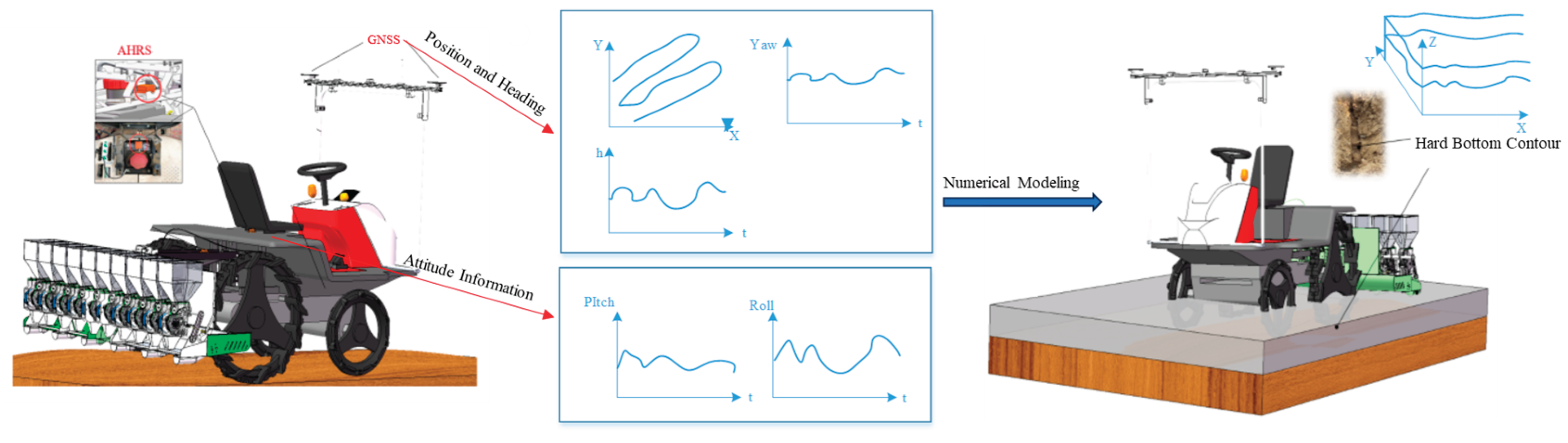
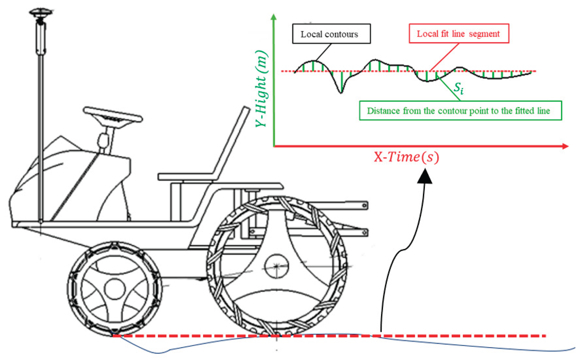
Using a wheeled agricultural machine equipped with an autonomous driving system as the mobile platform, a GNSS and an AHRS are installed on the machine's chassis. The GNSS measures the real-time spatial position and heading information of the machine during operation, while the AHRS measures the motion attitude of the chassis. A time-stamp synchronization method is employed to synchronously collect the machine's position and attitude data. During field operations, the wheels contact the hard bottom layer of the paddy field. Continuous contact points between the bottom of wheels and the hard bottom layer form a point cloud of the hard bottom contour. Based on measured position and attitude information—including the machinery's spatial position, heading angle, and chassis pitch angle—the Euler transformation method establishes a bottom of the wheel motion trajectory model in the global coordinate system [
8]. GNSS spatial positioning and orientation data, combined with AHRS roll and pitch attitude information, are processed through sensor calibration and outlier handling to reconstruct the hard-bottom contour terrain traced by the machine's wheels. A visualizable hard-bottom contour digital model is then constructed using a triangulated mesh method based on the collected point cloud. The designed agricultural machinery pose information and hard-bottom contour perception platform is illustrated in
Figure 1.
2.2. Correlation Analysis Method Between Agricultural Machinery Operational Motion States and Contour Feature Parameters
2.2.1. Method for Extracting Agricultural Machinery Operational Motion State Parameters
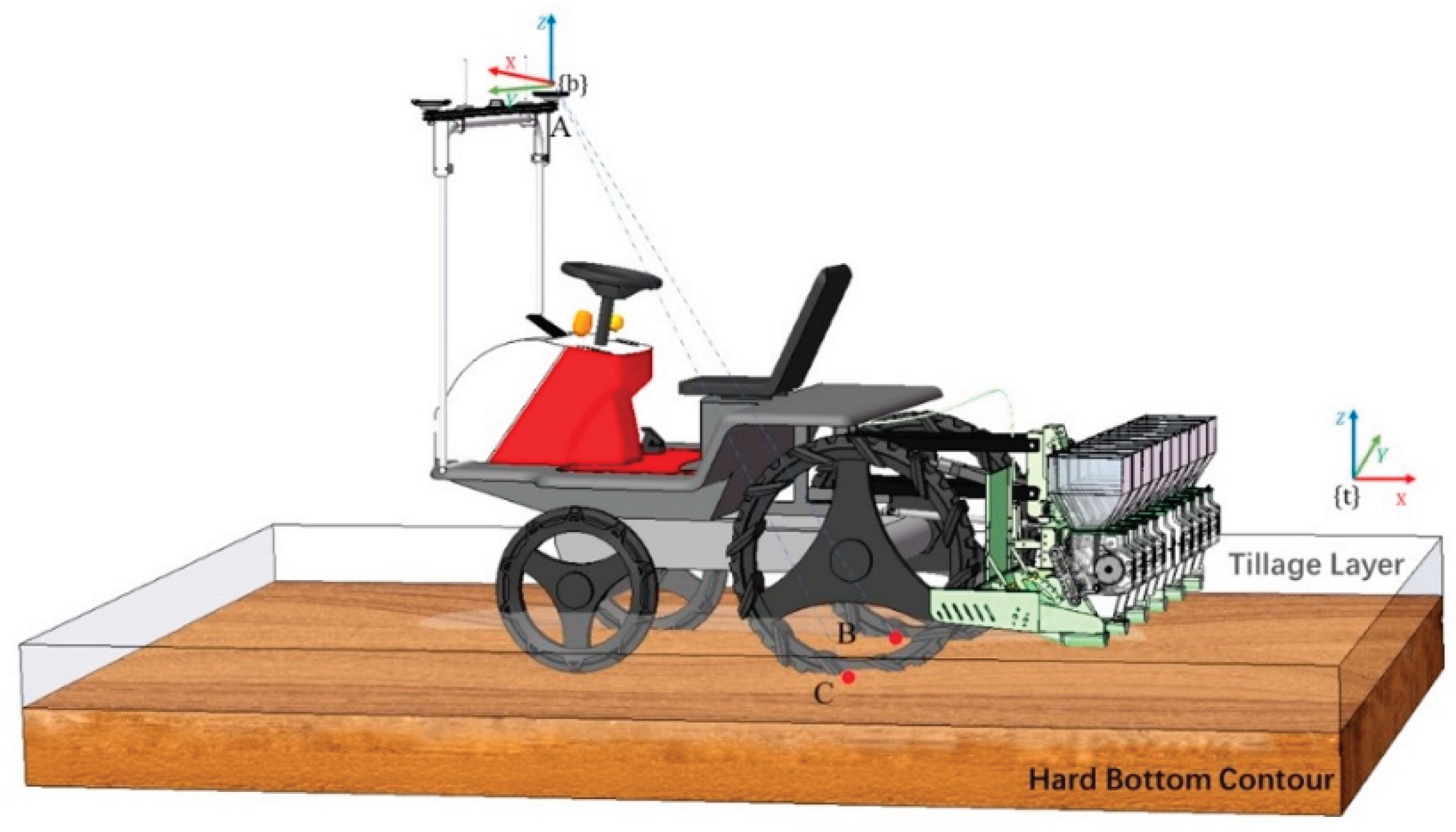
The onboard GNSS dual-antenna satellite positioning system enables the main antenna to capture the spatial position of the agricultural machinery antenna installation point within a local tangent plane coordinate system, along with the working speed and heading angle between the two antennas. The integrated AHRS system measures the pitch and roll angles of the agricultural machinery chassis. During actual operations, the agricultural machinery undergoes frequent attitude changes. The position of the main antenna cannot fully represent the machinery's motion state when it is not level. Therefore, the motion states of the bottom surfaces of the left and right rear wheels and the center of the rear suspension are used to express the machinery's true motion. By establishing a vehicle coordinate system, coordinate increments relative to the main antenna installation position are obtained for the bottom of the left and right rear wheels. Real-time motion information for the rear wheel bottoms is derived through continuous conversion based on the main antenna position and the vehicle's current attitude. The relationship between the local tangent plane coordinate system {t}, the vehicle coordinate system {b}, and the position of the rear wheel bottoms is illustrated in
Figure 2.
Due to the rotational relationship between the bottom of wheel and wheel hub, the effect of rotation on the bottom of wheel position must be considered. This involves analyzing the change in coordinate increments of the bottom of wheel within the vehicle body coordinate system during body pitch. The positional relationship during body pitch is illustrated in
Figure 3.
Let the right wheel's base point be
, with coordinates
in the vehicle body coordinate system. Expressed as a matrix:
Among these, denotes the distance between the two positioning antennas, represents the distance between the left and right wheel hubs, is the vertical distance from the antenna positioning center point to the right rear wheel hub D, and is the distance projected along the X-axis of the vehicle coordinate system from the antenna positioning center point to the right rear wheel hub D. , , and represent the incremental coordinates of the bottom of the wheel relative to the wheel hub in the x, y, and z directions of the vehicle coordinate system, respectively. denotes the rotation angle of the vehicle coordinate system relative to the local tangent plane coordinate system's X-axis, and is the wheel diameter.
Let the transformation matrix for converting point set coordinates in the vehicle body coordinate system to the local tangent plane coordinate system be
. The rotation matrix about the Z-axis is
, the rotation matrix about the Y-axis is
, and the rotation matrix about the X-axis is
. Then:
Taking the bottom of right wheel as the sampling point, let the position coordinates of the main antenna in the global coordinate system {e} be
eP
A(B, L, H). After Gauss projection transformation to the local tangent plane coordinate system {t}, the coordinates become
tP
A(x
At, y
At, z
At). Let the set of
tP
A coordinate points for point A of the main antenna in the local tangent plane coordinate system be
. and the coordinate set of the bottom of right wheel point in the local tangent plane coordinate system after Euler transformation is
. Then:
Similar to setting the left wheel center point as
, the coordinates of
in the vehicle coordinate system are expressed as a matrix:
The set of points
obtained by Euler transformation of the base point coordinates of a revolver in the local tangent plane coordinate system satisfies:
Let the center point of the rear axle be
. The coordinates of
in the vehicle coordinate system are expressed as a matrix:
The ePA point cloud undergoes Gaussian projection and Euler transformation to obtain the coordinate matrices , , and for the right rear wheel bottom layer, left rear wheel bottom layer, and rear axle center in the local tangent plane coordinate system. Based on these coordinate positions, the displacement, velocity, and acceleration of the agricultural machinery's wheel bottoms and rear axle center are derived. These provide the motion-related input variables for analyzing how hard-surface contour excitation influences the agricultural machinery's pose.
By applying differential operations to the positional time series data from the bottom of the left and right wheels and the center of the agricultural machinery's rear axle, the corresponding kinematic parameters of the machinery can be derived. Specifically, performing first-order differentiation on the displacement time series of the left and right wheel bottoms yields the linear velocity of the right wheel bottom, the linear velocity of the left wheel bottom, and the velocity of the agricultural machinery's rear axle center, respectively.
Taking the calculation of the right wheel's baseline motion parameters as an example, let the right wheel's baseline velocity be
and its baseline acceleration be
. Using a discrete difference form, the calculation yields:
were,
n denotes the time step index, and Δ
t represents the sampling interval. For the 10 Hz frequency data acquisition in this paper, this value is 0.1 seconds.
Similarly, the linear velocity
and linear acceleration
of the revolver can be calculated as follows:
Center vehicle velocity
, center vehicle acceleration
, where:
To represent the instantaneous directional change during agricultural machinery movement, the lateral bottom of the wheel velocity difference
and acceleration difference
are introduced, where:
Based on data acquired from satellite positioning and attitude sensors, a complete mathematical mapping relationship is established through differential operations. This relationship transforms observational data from various parts of the agricultural machinery into parameters describing the motion state of the bottom of the wheels and the center of the rear axle. This provides input for analyzing the relationship between the motion state of the agricultural machinery and the contour characteristics of the hard bottom layer.
2.2.2. Method for Extracting Contour Feature Parameters of Hard Bottom Layer
Agricultural machinery operates on hard bottom layers, with wheels exerting force upon the hard bottom layer contour. Due to the absence of shock-absorbing suspension on the rear axle, the contour surface of the hard bottom layer directly impacts the vehicle's wheels. This force induces displacement and attitude changes in the wheels contacting the hard bottom layer. By utilizing GNSS position and AHRS attitude data from the machinery, discrete point clouds
(Equation 6) and
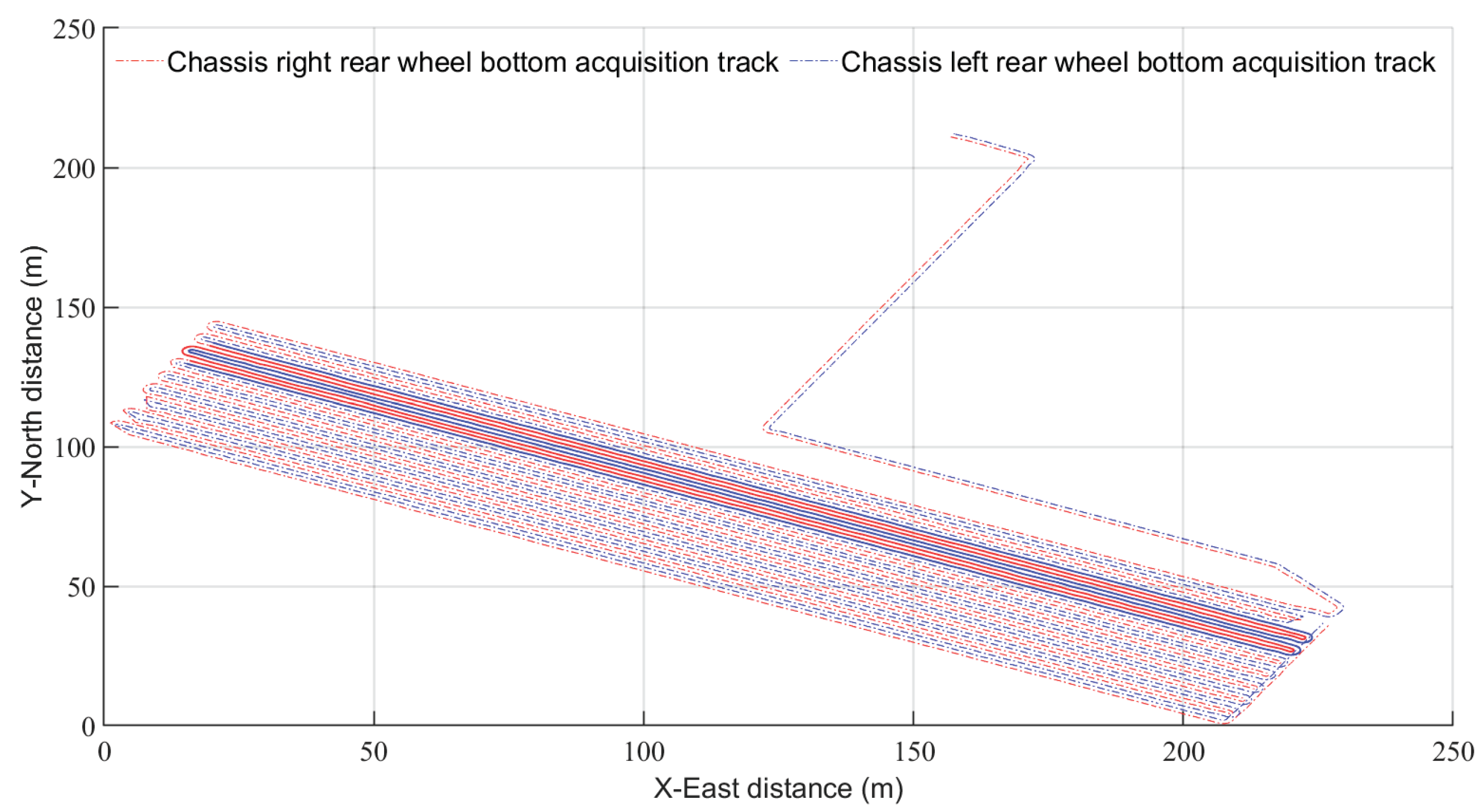
(Equation 8) representing the bottom of left and right wheels are reconstructed. Through automatic sensor calibration, outlier removal, and 3D spline curve denoising of the contour trajectory, a digital model of the hard bottom layer contour traversed by the machinery is constructed. In practical field operations, agricultural machinery primarily follows planned straight sections. The quality of straight-line segment operations critically impacts overall field performance. To extract representative hard bottom layer trajectory patterns, straight-line segments were isolated from the full-field hard bottom layer contour. The full-field wheel-bottom trajectory is illustrated in
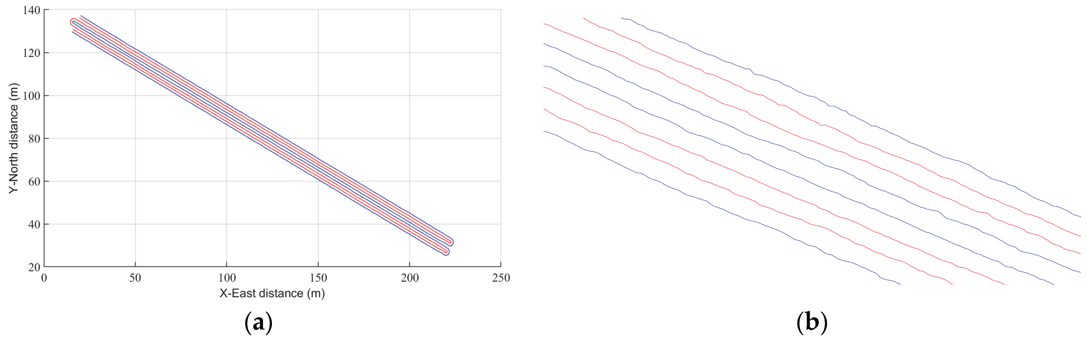
Figure 4. The actual hard bottom layer contours of the left and right wheels of the agricultural machinery were isolated. Continuous scattered points were then fitted with spline curves to form smooth hard bottom layer contours, as shown in
Figure 5.
Based on the coordinate points connecting the 3D spline curve of the hard bottom layer contour, isolate the contour points of the hard bottom layer in contact with the bottom of left wheel. In the local tangent plane coordinate system, the X-axis coordinate value is , Y-axis coordinate value , and Z-axis coordinate value . Additionally, the X-axis coordinate value , Y-axis coordinate value , and Z-axis coordinate value of the hard bottom layer contour points contacting the bottom of right wheel in the local tangent plane coordinate system, along with the Z-axis coordinate height difference between the hard bottom layer contours contacting the bottom of left and right wheels.
To further analyze the impact of localized characteristics of the hard bottom layer on the movement state of agricultural machinery, the surface roughness of the hard bottom layer is introduced to represent the degree of localized undulation. Based on the contour information of the hard bottom layer, a section spanning the agricultural machinery's wheelbase length was selected locally. A straight line was fitted using the least squares method, and the height of each point relative to this fitted line was calculated. The relationship between the hard bottom layer contour, the locally fitted line segments, and the height of contour points relative to the fitted line is illustrated in
Figure 6.
Let the coefficient of the linear term (slope) of the locally fitted line based on the least squares method be
, the constant term (intercept) be
, and the distance from the th contour point within the local region to the fitted line be
. Then:
where,
denotes the distance from the i-th contour point to the fitted straight line;
represents the index of the i-th contour point;
denotes the height of the i-th contour point.
Let the local surface roughness at the j-th point on the hard bottom layer be denoted as
, calculated using the following formula:
where,
represents the sample size within the specified range.
By performing a traversal calculation on the hard-bottom contour collected from the field according to Equation (19), the continuous surface roughness characteristic values of the hard-bottom contour traversed by the agricultural machinery can be obtained.
2.2.3. Correlation Impact Analysis Method
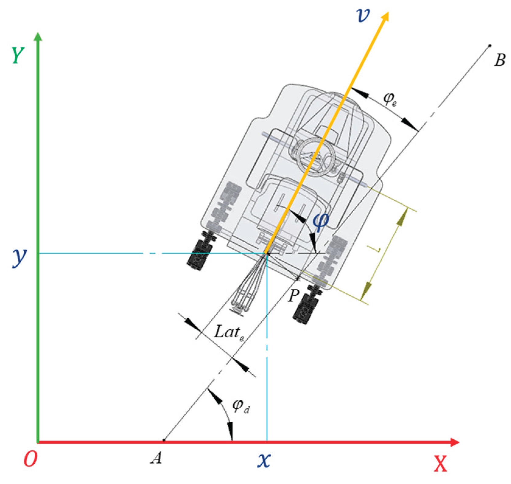
When agricultural machinery performs path-following operations, the degree of deviation in vehicle posture from the planned path serves as a key parameter for evaluating the operational quality of autonomous agricultural machinery and determining decision-control output. To analyze how the motion state parameters and hard bottom layer contour feature parameters of agricultural machinery affect the deviation of its posture from the planned path, real-time position and heading are obtained via GNSS. These are then compared with the expected values of the planned path to derive the perpendicular distance between the vehicle position and the expected path (lateral deviation) and the angular difference between the vehicle direction and the expected path direction (heading deviation). Schematic diagrams of lateral deviation and heading deviation are shown in
Figure 7.
The installed GNSS and AHRS systems continuously capture real-time position and attitude parameters of the agricultural machinery, including antenna elevation, velocity, heading angle, pitch angle, and roll angle. Building upon the sensor-derived data, the agricultural machinery operational motion state parameter extraction method described in
Section 2.2.1 is employed. Through Euler transformation, the following motion state parameters are obtained: the bottom of left wheel velocity, the bottom of right wheel velocity, the bottom of left-right wheel velocity difference, left wheelbase acceleration, right wheelbase acceleration, left-right wheelbase acceleration difference, vehicle center velocity, and vehicle center acceleration.
Section 2.2.2's hard bottom layer contour feature extraction method is used to obtain the 3D coordinates of contact points between the agricultural machinery and the hard bottom layer contour, along with local elevation differences and surface roughness characteristics. A segmented straight working path was selected. Continuous data sets synchronously collected by the vehicle-mounted autonomous driving system—including vehicle pose sensors and operational parameters—were used as the test dataset. Numerical sets for hard bottom layer contour features and agricultural machinery pose parameters were calculated. The lateral deviation and heading deviation recorded during operation were analyzed in relation to the hard bottom layer contour feature parameters and agricultural machinery pose parameters, respectively. To quantify the linear correlation strength and direction between hard bottom layer contour features and agricultural machinery motion parameters as multivariate pairwise continuous variables, this study employs the classical Pearson correlation analysis method. This method calculates the correlation coefficient between each pair of variables by computing the ratio of the covariance between the agricultural machinery motion parameters and the hard bottom layer contour feature parameters to their respective standard deviations multiplied by the position deviation and heading deviation. The calculation formula is as follows:
In the equation, denotes the sequence number of the variable type representing the contour feature parameter of the hard bottom layer for agricultural machinery motion parameters; denotes the sequence number of the deviation type for agricultural machinery motion; denotes the correlation coefficient between the two variables; denotes the covariance between the and variables; and denote the standard deviations of the and variables, respectively.
The correlation coefficient ranges from -1 to 1, where 0 indicates no linear relationship between two variables, 1 indicates perfect positive correlation, and -1 indicates perfect negative correlation. By observing the degree of correlation, significant factors influencing lateral deviation and heading deviation during agricultural machinery movement are analyzed and extracted. Based on the identified significant factors, field experiments are conducted to analyze how the hard bottom layer contour characteristics affect the position and orientation of agricultural machinery.
2.3. Extraction of Agricultural Machinery States During Typical Bogging Processes
During paddy field operations, agricultural machinery often becomes bogged down in mud or soft soil while maneuvering at field edges or working on an unknown hard bottom layer. Unable to extricate itself, the vehicle becomes stuck, severely reducing operational efficiency. This issue is particularly critical during unmanned intelligent farming operations, as it necessitates halting the work program and disrupts continuous operation. Field observations during the application and promotion of intelligent farm machinery in paddy fields reveal that vehicle entrapment predominantly occurs when the destruction of the hard bottom layer increases wheel trapping depth. Farm machinery wheels become embedded in this layer, unable to extricate themselves through their own propulsion. This typical type of paddy field entrapment is related to the depth and local characteristics of the hard bottom layer. A schematic illustration of vehicle entrapment is shown in
Figure 8.
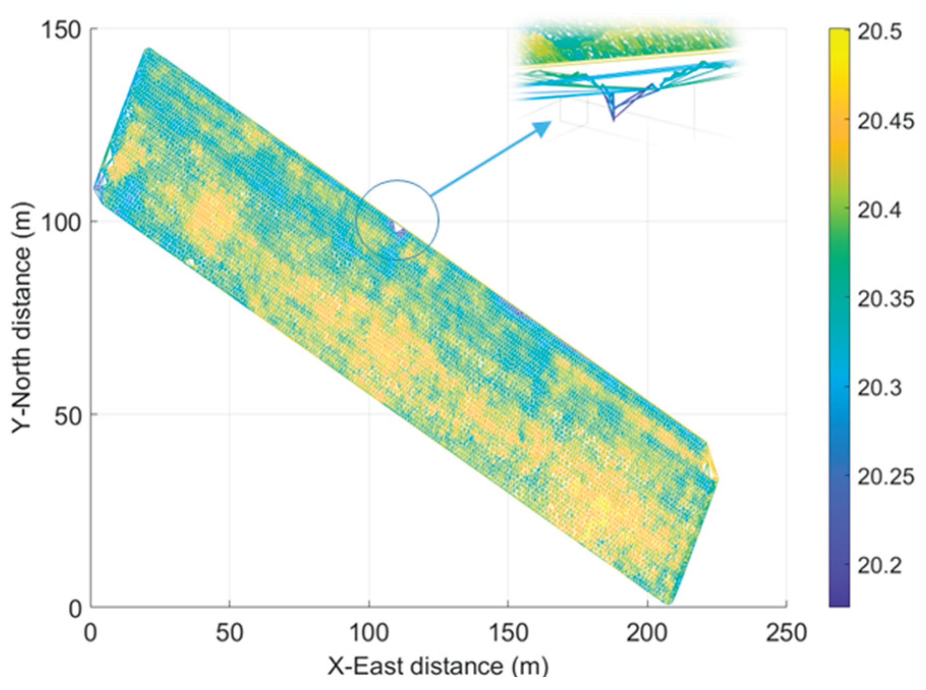
To analyze the typical vehicle entrapment process of agricultural machinery under hard bottom layer conditions, operational data from production trials exhibiting typical entrapment scenarios were extracted for analysis. A digital model of the hard bottom layer in the entrapment field was constructed using a hard bottom layer digital modeling method. Based on typical bogging incidents occurring during actual agricultural machinery operations, the hard bottom layer contour was captured and its characteristic parameters were extracted using the method described in
Section 2.2.2. This process yielded a localized contour model of the hard bottom layer and its characteristic parameters under typical bogging conditions. The resulting bogging contour model and its locally magnified region are shown in
Figure 9.
To analyze the dynamic characteristics of the hard bottom layer contour before and after the moment of agricultural machinery becoming stuck, the contour feature parameters of the hard bottom layer were extracted from data collected within 15 seconds before and after the incident. The data system was configured with a sampling frequency of 10 Hz, enabling the extraction of 300 data sets for analysis. The study focused on the contour height at the tire-hard bottom layer interface and the local roughness of the hard bottom layer. Through numerical analysis, a dynamic variation model of the hard bottom layer contour characteristics under typical entrapment scenarios was constructed.
3. Results and Discussion
3.1. Test Scenario
3.1.1. Paddy Field Operation Test Scenario
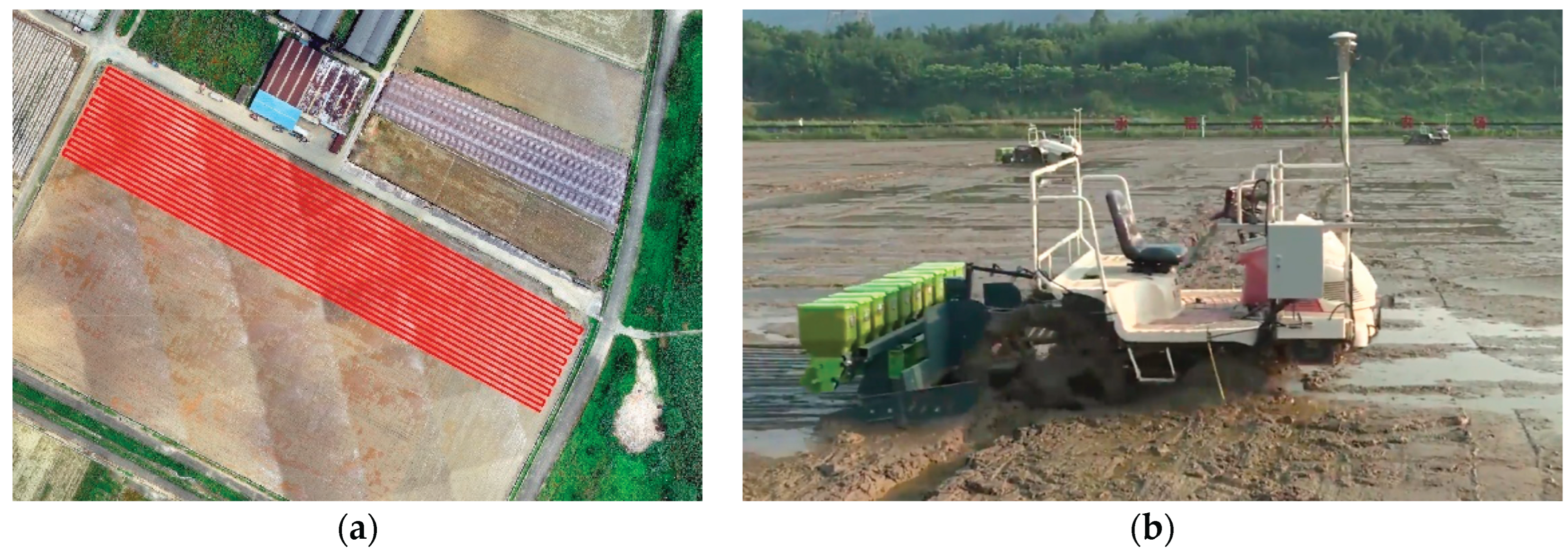
An unmanned direct-seeding machine was deployed in rice fields at Guangzhou's Zengcheng District unmanned farm. The machine integrated agricultural machinery position and attitude data, and hard bottom layer information collection system integrated onto the unmanned rice direct seeder to collect real-time position and attitude data. Utilizing hard bottom layer contour acquisition and feature extraction methods, corresponding contour information was synchronously obtained during machinery movement. The unmanned rice direct seeder performed automated mechanical seeding while concurrently collecting hard bottom layer and mud surface data. The planned working path of the direct seeder is shown in
Figure 10(a), and the operational site is depicted in
Figure 10(b).
3.1.2. Hard Road Surface Test Scenario
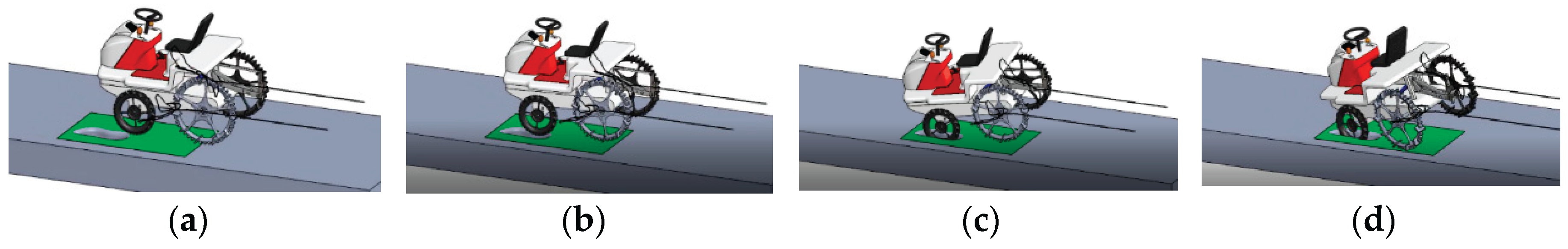
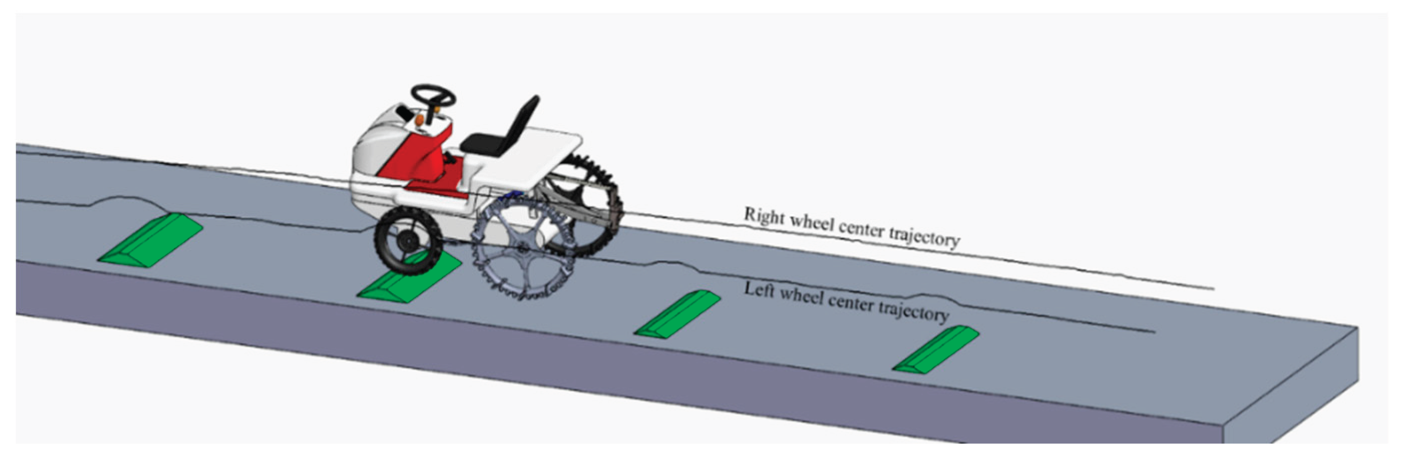
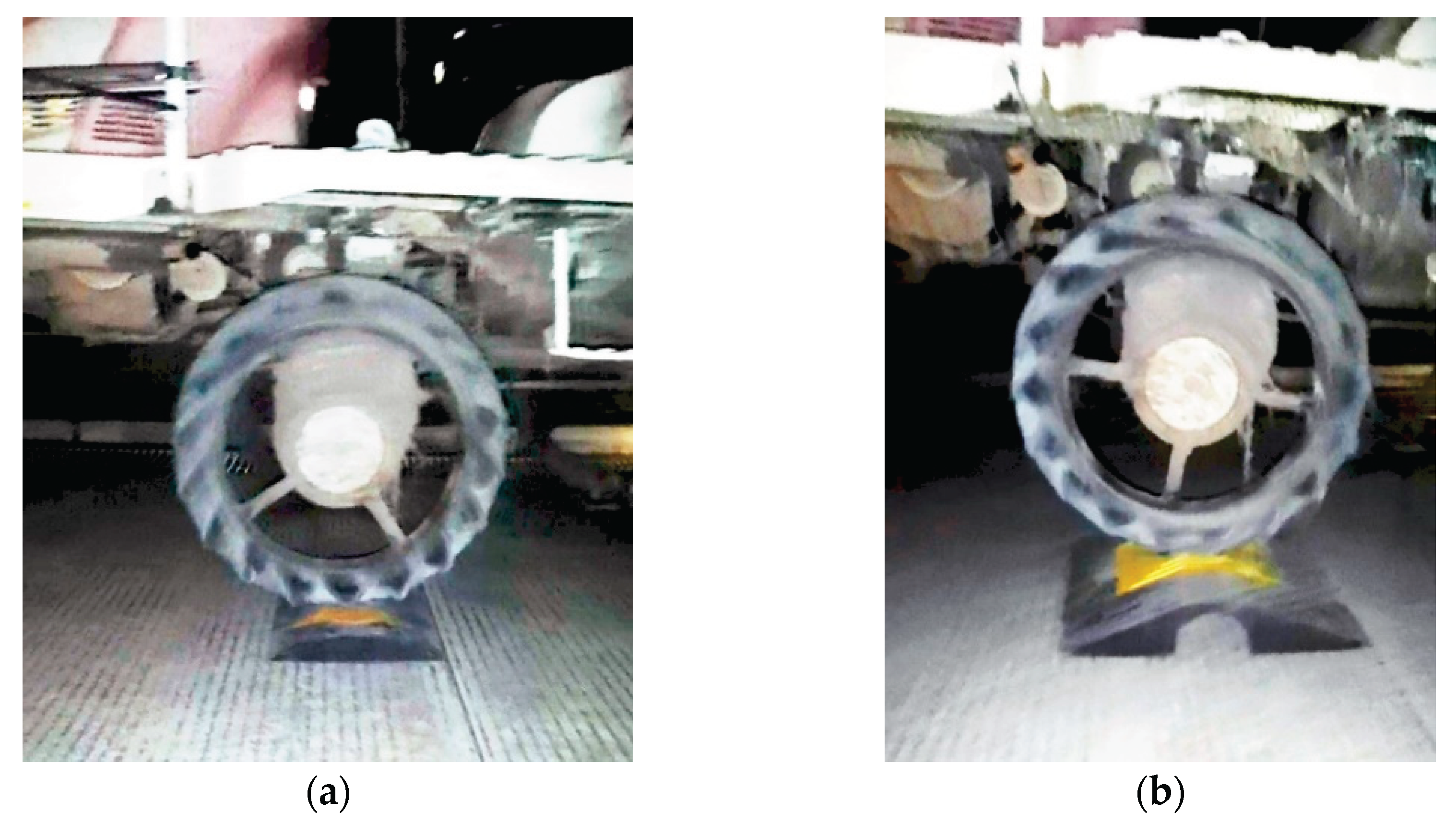
Furthermore, to analyze the impact of agricultural machinery movement when traveling along a hard bottom layer contour with a known fixed elevation difference, two sets of 5cm-high trapezoidal ridges and two sets of 10cm-high trapezoidal ridges were laid at equal intervals along the planned agricultural machinery track on a hard cement road. Using automatic straight-line driving mode, the machinery's single-side wheels directly rolled over the ridges, causing lateral tilt. The machinery's position and orientation data were collected to analyze the impact of fixed-height ground contours on its posture through experimental evaluation. The experimental setup is illustrated in
Figure 11, while the actual field test site is shown in
Figure 12.
3.2. Analysis of the Relationship Between Agricultural Machinery Movement State and Hard Bottom Layer Characteristic Parameters
3.2.1. Correlation Analysis Results
During paddy field operation trials, the contour characteristics of the paddy field hard bottom layer and the impact of agricultural machinery movement were analyzed. Data collected from paddy field operation scenarios were selected and segmented into straight operation path segments. A dataset comprising 3,091 sets of synchronously collected data from vehicle-mounted position and attitude sensors and operation parameters via the vehicle-mounted autonomous driving system was used as the test dataset. Employing the parameter extraction method described in
Section 2.2, calculating parameter sets for hard bottom layer contour characteristics and agricultural machinery attitude. These parameters were then analyzed against lateral deviation and heading deviation data collected during operations, with results presented in
Table 1.
The correlation strength and direction between the hard-bottom contour features and the agricultural machinery's position and attitude parameters were determined by combining the results of significance tests and correlation coefficients. The lateral deviation and heading deviation during straight-line operation of the agricultural machinery showed extremely significant correlations with the Z-axis height and height difference of the hard-bottom contour at the bottom of left and right wheels, respectively. Simultaneously, both deviations exhibited extremely significant correlations with the local roughness of the hard-bottom contour. The lateral deviation also exhibited extremely significant correlation with the linear velocity difference between the bottom of left and right wheels. The Pearson correlation analysis results provide a reference basis for further analysis of the agricultural machinery's motion and posture response under hard-surface layer excitation.
3.2.2. Results of Straight-Line Driving Test on Rigid Pavement with Fixed Elevation Difference
1) Fixed wheel angle through the ridge test
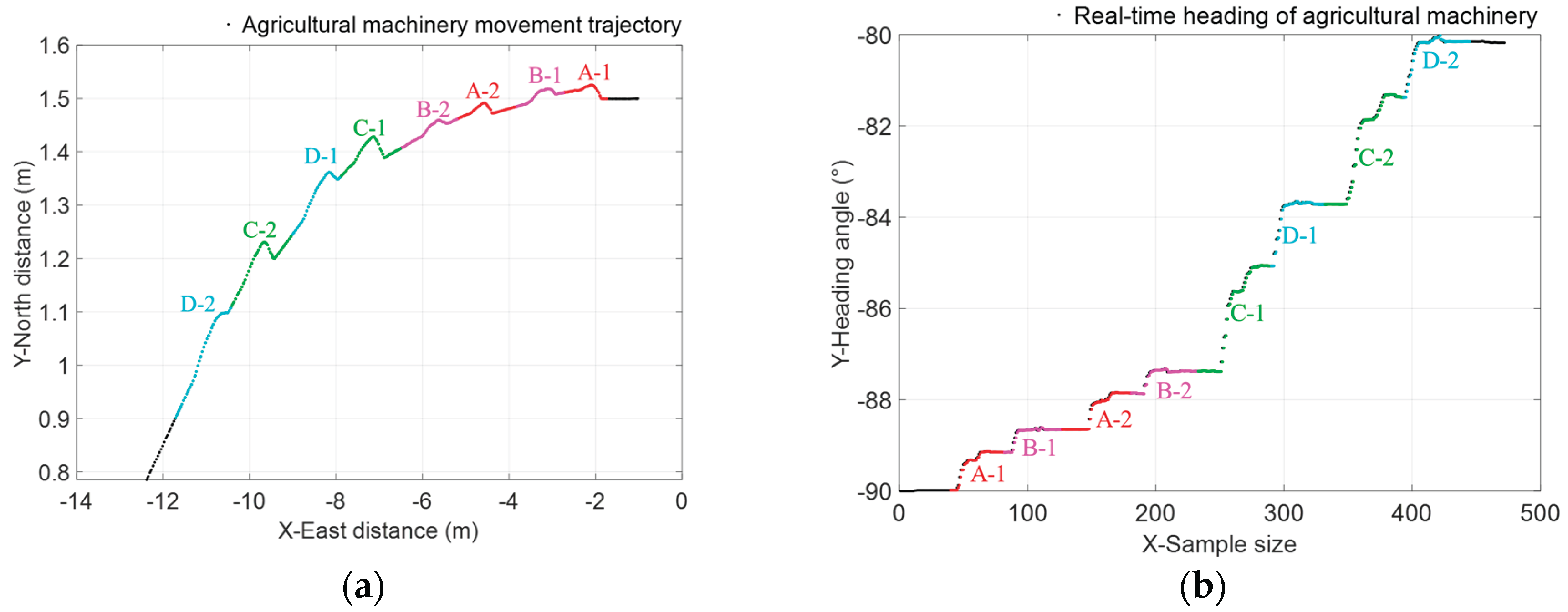
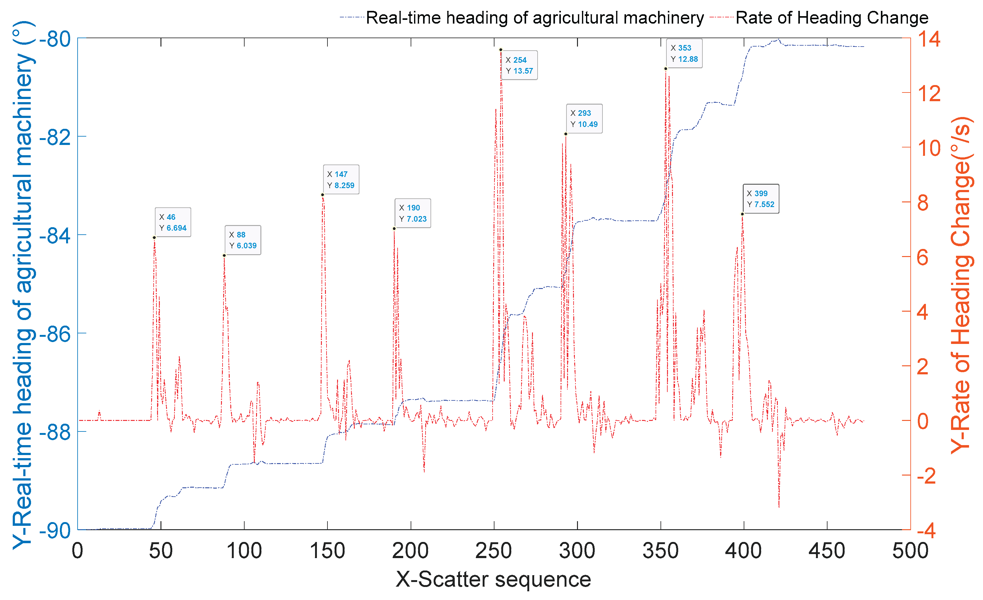
Using the fixed wheel angle of agricultural machinery during straight-line travel, a continuous ridge-crossing test was conducted. By obtaining rear wheel center trajectory data, the heading and heading change rate of a single wheel crossing ridges were analyzed. The front wheels of the rice transplanter's mobile chassis had a diameter of 650 mm, while the rear wheels measured 950 mm in diameter. The speed was set to the field operation speed of 1 m/s. The front and rear wheels traversed two 5 cm-high ridges and two 10 cm-high ridges respectively, comprising a total of eight stages designated as A-1, B-1, A-2, B-2, C-1, D-1, C-2, and D-2. The planar trajectory of the agricultural machinery traversing the ridge platform during all stages is shown in
Figure 13(a), while the heading changes are depicted in
Figure 13(b). Simultaneously, the heading and heading change rate during the machinery's passage over the ridge platform were acquired, with the results presented in
Figure 14. The stage numbers and descriptions for the entire test process are detailed in
Table 2.
As shown in
Figure 13 and
Table 2, the trajectory tracking results for single-wheel crossing of ridges indicate that when both front and rear wheels continuously traverse a ridge, the agricultural machinery's heading persistently deviates toward the side with the ridge. The heading variation range when crossing a 5 cm-ridge was 0.48°-0.85°, while crossing a 10 cm-ridge resulted in a variation range of 1.17°-2.40°. The heading change caused by a 10 cm obstacle was 2-3 times that of a 5 cm one, indicating that ridge height is the primary influencing factor—consistent with the correlation analysis results.
As shown in
Figure 14 and
Table 2, from the perspective of heading change rate, the front wheel (diameter 0.65 m) exhibited an average heading change rate of 7.48°/s when traversing a 5 cm obstacle, while the rear wheel (diameter 0.95 m) averaged 6.53°/s. This indicates a reduction of approximately 12.6% in the rear wheel's heading change rate compared to the front wheel. When traversing a 10 cm ridge, the front wheel exhibited a phase-average heading rate of 13.23°/s, while the rear wheel recorded 9.02°/s, indicating a reduction of approximately 31.8% in the rear wheel's heading rate compared to the front wheel. Larger-diameter wheels demonstrate greater stability when traversing ridges than smaller wheels, a characteristic that becomes more pronounced when navigating higher ridges.
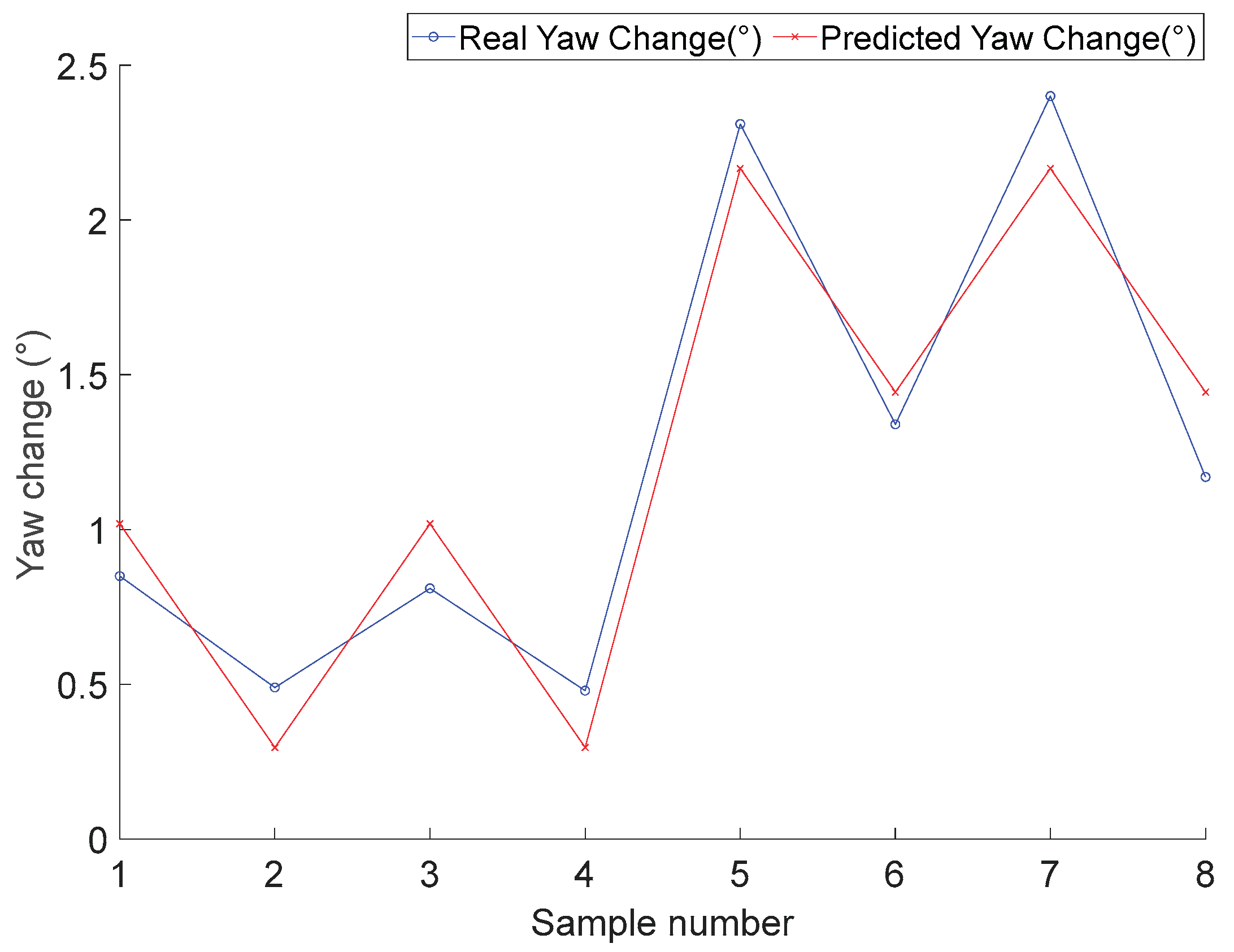
A regression model was developed with ridge height and wheel diameter as independent variables, and the heading change as the dependent variable, as follows:
where
represents the heading change value,
represents the ridge height, and
represents the wheel diameter.
The regression model achieved a coefficient of determination (R²) of 0.92356 and a sum of squared errors (SSE) of 0.30436. The comparison between the measured and predicted heading change values is presented in
Table 3 and
Figure 15.
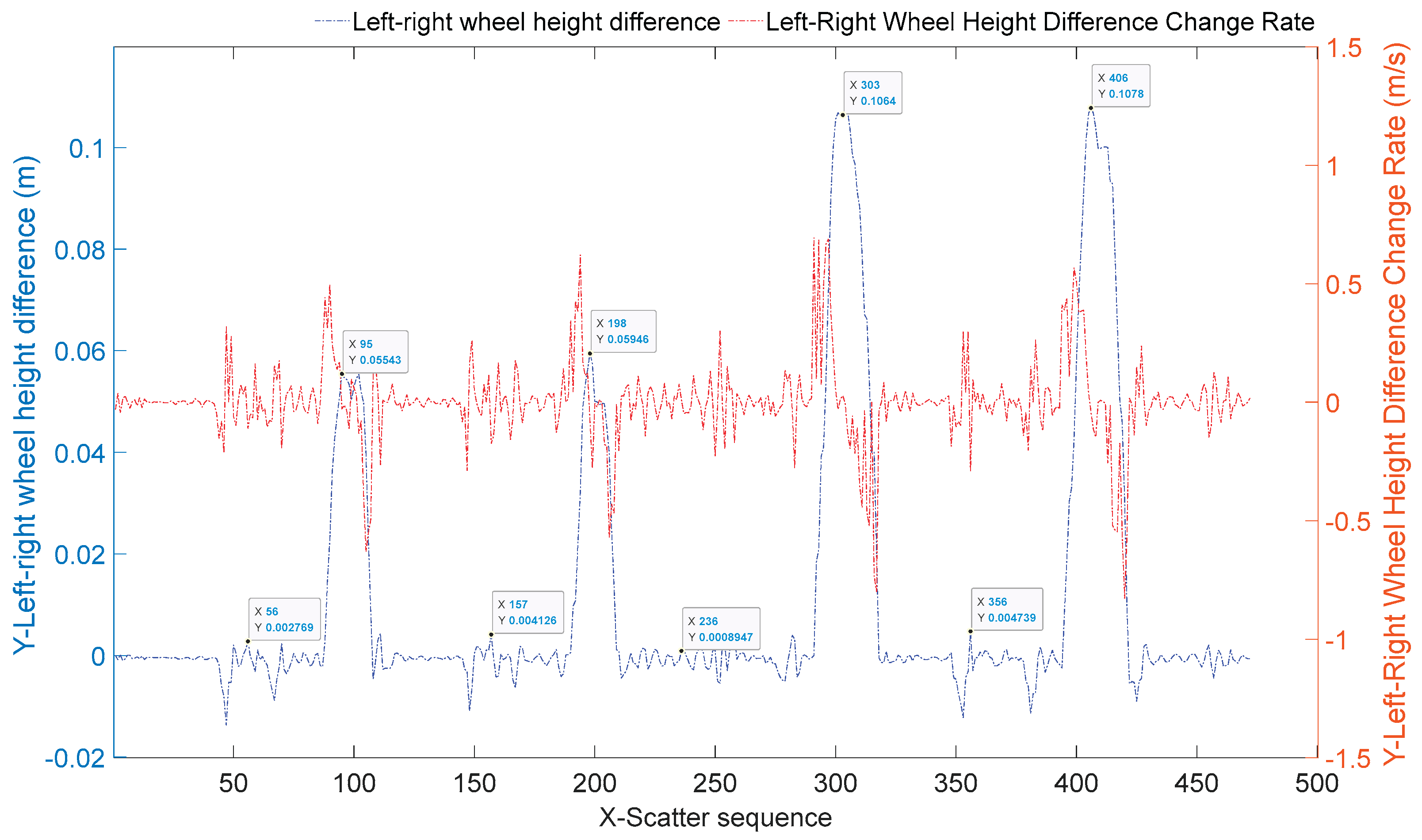
To further observe the dynamic process of height differences and their rate of change between the left and right rear axles of agricultural machinery caused by the ridge, the height differences and their rates of change at each pass stage were extracted, as shown in
Figure 16.
As shown in
Figure 16, whether traversing a 5 cm or 10 cm ridge, the front wheels exhibit minimal impact on the rear axle height difference (within 1 cm). However, when the rear wheels pass over the ridge, the rear axle height difference closely matches the ridge height, measuring 5.5 cm, 5.9 cm, 10.6 cm, and 10.8 cm respectively. Therefore, the front suspension system effectively counteracts terrain effects on the vehicle body when the front wheels traverse the ridges. The rear axle, lacking suspension damping, perceives the actual contour features of the hard subsoil layer when the rear wheels pass over it. The primary factor influencing the roll attitude of the agricultural machinery lies in the terrain characteristics encountered during rear-wheel traversal. Consequently, when considering control compensation for the machinery, the focus should be on the rear wheels and the terrain features they encounter during passage.
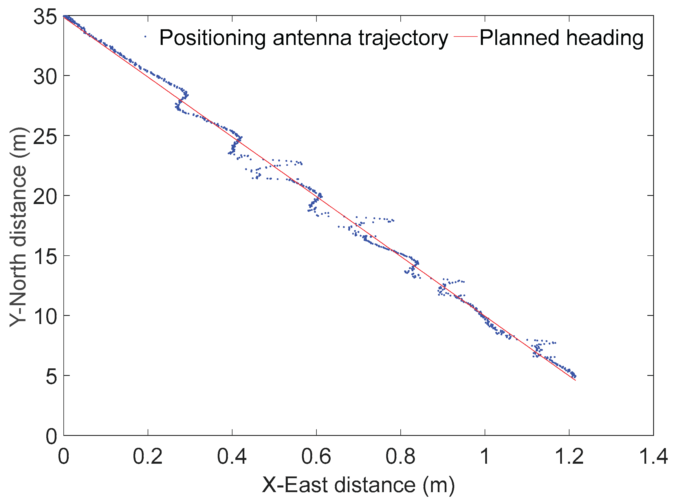
2) Straight-line autonomous driving passes ridge test
During straight-line autonomous driving trials on ridges, the agricultural machinery traversed four ridges of identical specifications using straight-line assisted driving. The planar trajectory of the positioning antenna is shown in
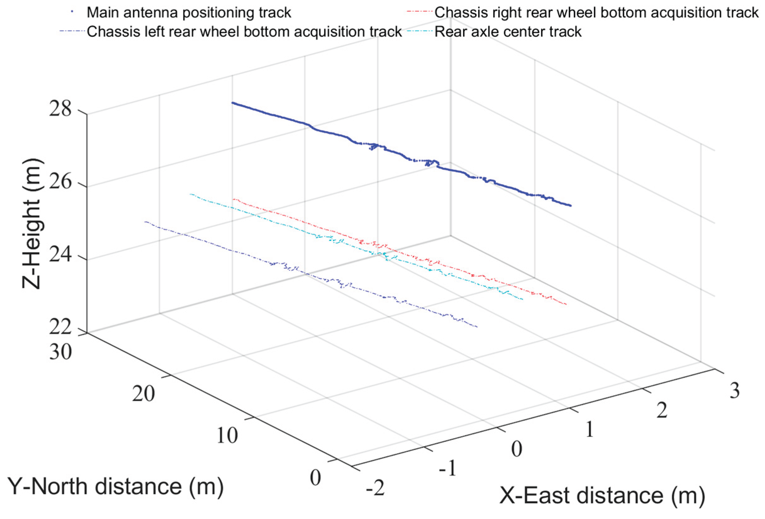
Figure 17. Using the sensor data calibration method(Tu et al., 2023), the roll system error was determined to be -2.429°, the pitch system error was 0.846°, and the heading system error was -1.103°. The rear axle center and bottom of the wheel trajectories are shown in
Figure 18.
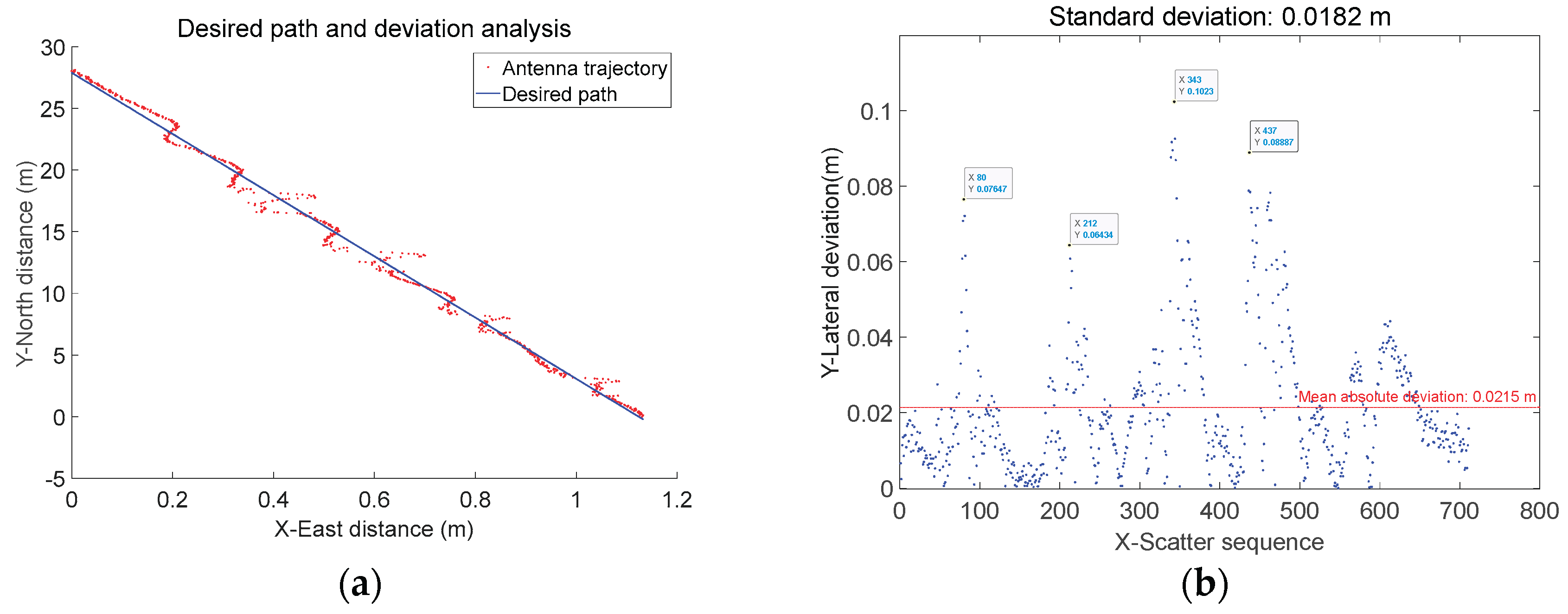
Based on the acquired positioning data, analyze the deviation of the antenna from the expected path as the agricultural machinery passes through each ridge. Combined with the acquired vehicle posture data, determine the deviation of the center of the rear axle and the center of the line connecting the bottom of left and right wheels from the expected path. The acquired antenna trajectory and its lateral deviation are shown in
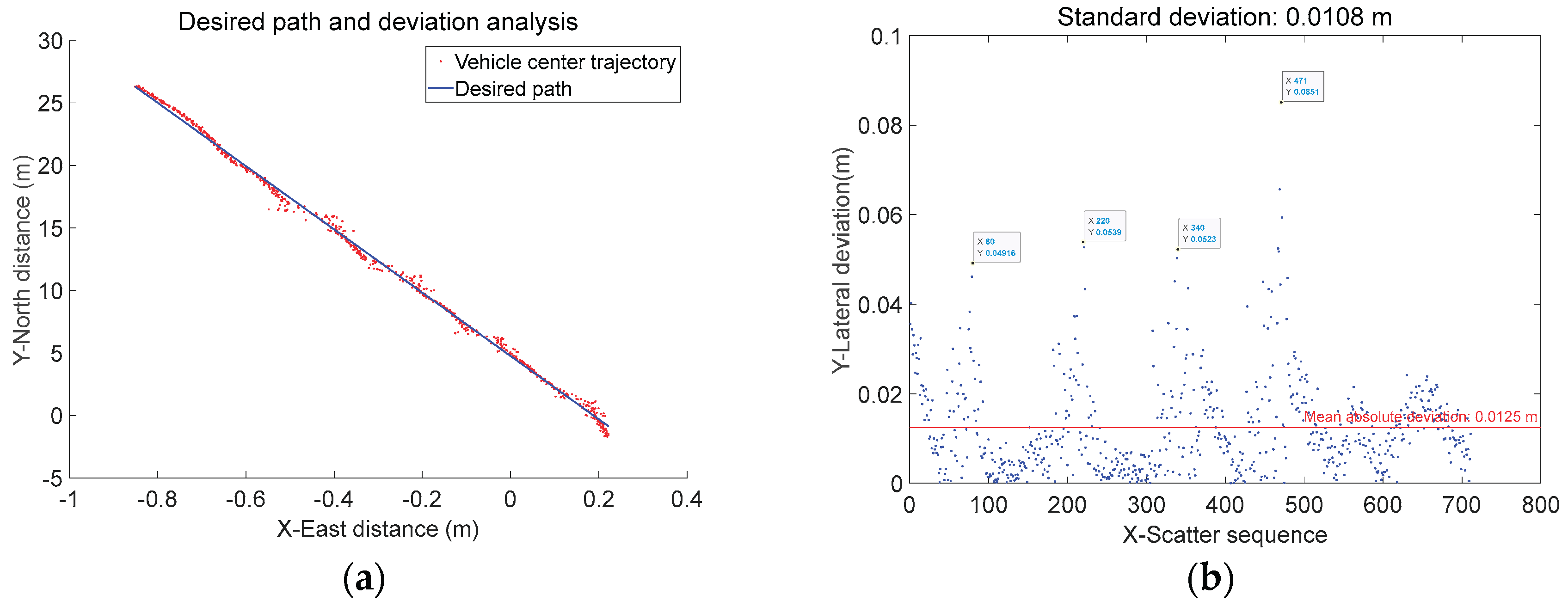
Figure 19. The acquired rear axle center trajectory and its lateral deviation are shown in
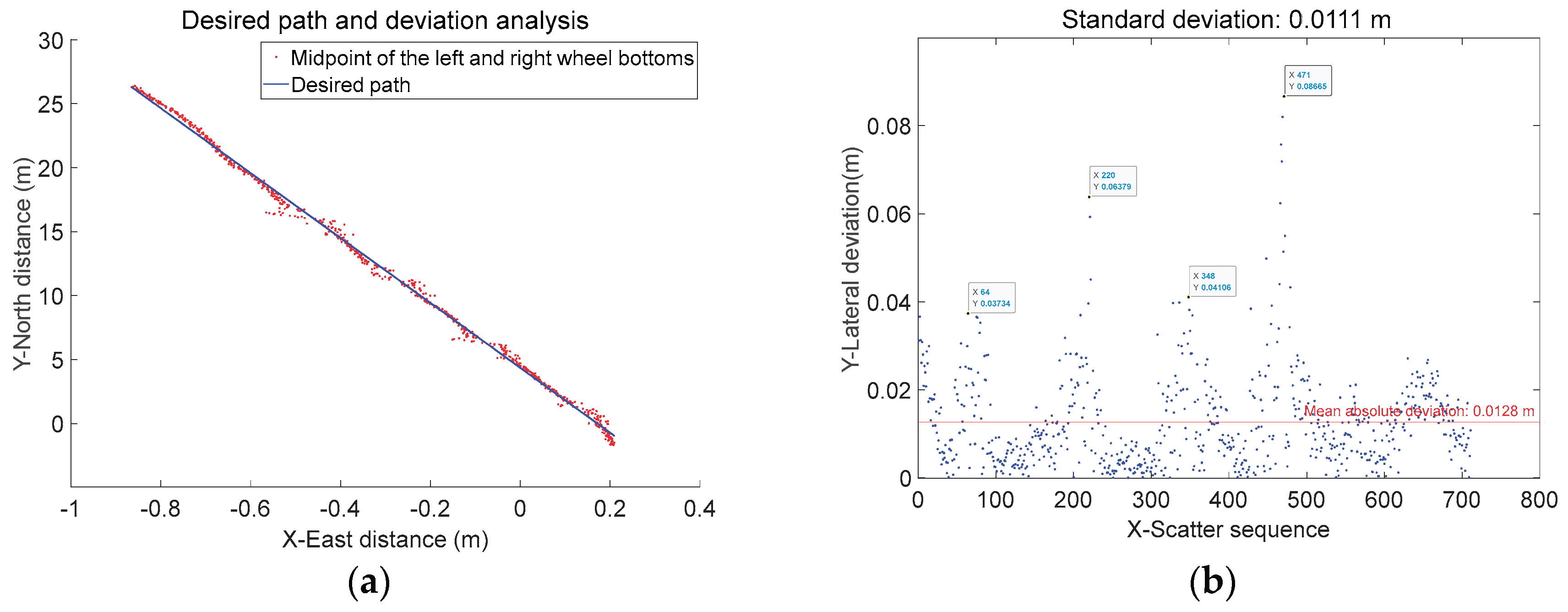
Figure 20. The acquired centerline trajectory of the bottom of left and right wheels and its lateral deviation are shown in
Figure 21.
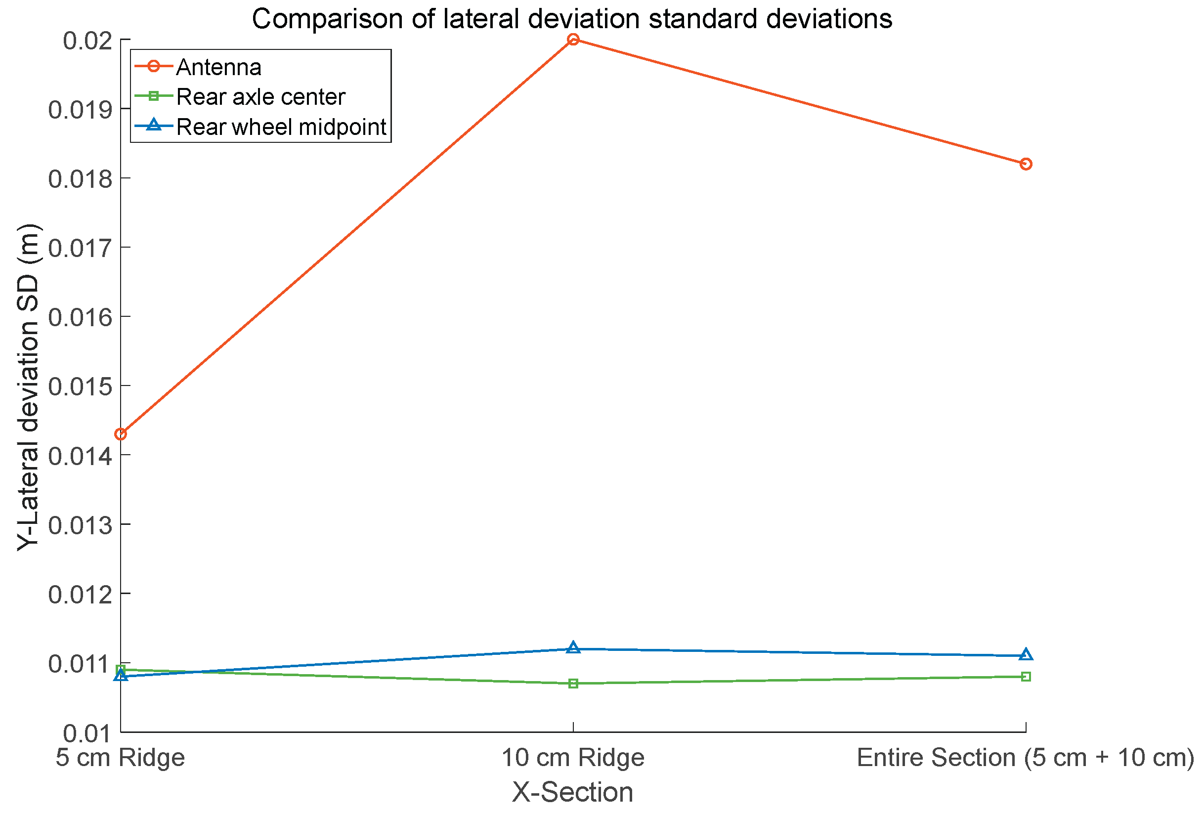
Results indicate that when traversing a 5 cm ridge section, the standard deviation of antenna lateral deviation was 0.0143 m, the standard deviation of rear axle center lateral deviation was 0.0109 m, and the standard deviation of left/right wheelbase center lateral deviation was 0.0108 m. When traversing the 10 cm ridge section, the standard deviation of antenna lateral deviation was 0.0200 m, the standard deviation of rear axle center lateral deviation was 0.0107 m, and the standard deviation of left/right wheelbase center lateral deviation was 0.0112 m; During the entire passage over 5cm and 10cm ridges, the standard deviation of the antenna lateral deviation was 0.0182 m, the standard deviation of the rear axle center lateral deviation was 0.0108 m, and the standard deviation of the left and right wheelbase center lateral deviation was 0.0111 m. Detailed information is shown in
Table 4 and
Figure 22.
As shown in
Table 4 and
Figure 22, when the agricultural machinery traversed 5 cm and 10 cm ridges respectively, the standard deviation of the positioning antenna heading deviation increased from 0.0143 m to 0.0200 m—nearly doubling. Meanwhile, the standard deviation of the heading for the attitude-corrected rear axle center and bottom of the wheel center remained virtually unchanged at approximately 0.01 m. This indicates that single-side passage over ridges causes lateral displacement of the higher-positioned antenna, while the machine itself does not experience lateral slip. The attitude-corrected rear axle center and bottom of the wheel center more accurately represent the machine's true real-time position and its actual deviation from the planned path.
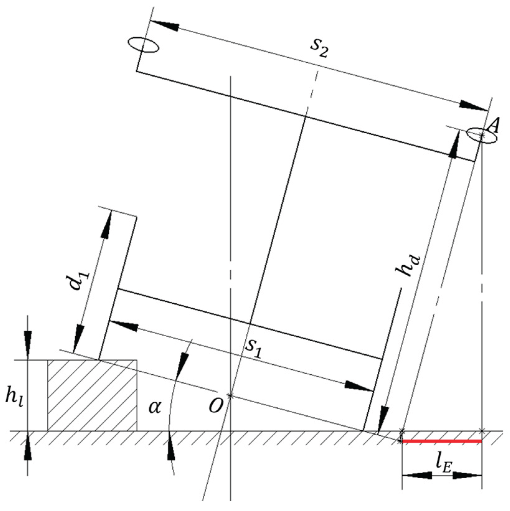
The lateral roll angle generated by the height difference between the left and right wheels of the agricultural machinery can be visualized from the rear view as the machinery rotating about the center point O at the base of the left and right wheels, as shown in
Figure 23.
Based on geometric relationships, the theoretical model for the antenna position deviation relative to the horizontal plane during agricultural machinery rollover is as follows:
In the equation, represents the vehicle roll angle caused by the height difference between the left and right wheels, denotes the height difference between the left and right wheels, indicates the rear track width of the agricultural machinery, shows the offset of the antenna position relative to the horizontal plane during roll, is the height of the antenna above the bottom of wheel, and is the symmetrical mounting distance between the dual antennas.
From the theoretical model Equation (23) and numerical results (
Table 4 and
Figure 22) for antenna position deviation relative to horizontal during the entire process of agricultural machinery rolling over ridges, it can be observed that the hard bottom layer contour significantly affects the lateral deviation of the positioning antenna. The deviation of the antenna position from the horizontal during machine rollover is proportional to the height difference between left and right wheels and the installation height of the antenna relative to the bottom of wheel. Specifically, when the machine rolls 1.91 degrees and 3.81 degrees over the tested 0.05 m and 0.1 m high ridges, the antenna position deviates 0.083 m and 0.166 m from the horizontal, respectively. After attitude correction calculations, the lateral deviation accuracy of the rear axle center and left/right wheel bottom centers relative to the positioning antenna improved by 40.7% and 39.0%, respectively.
3.3. Analysis of the Impact of Paddy Field Hard Bottom Layer on Typical Agricultural Machinery Bogging Incidents
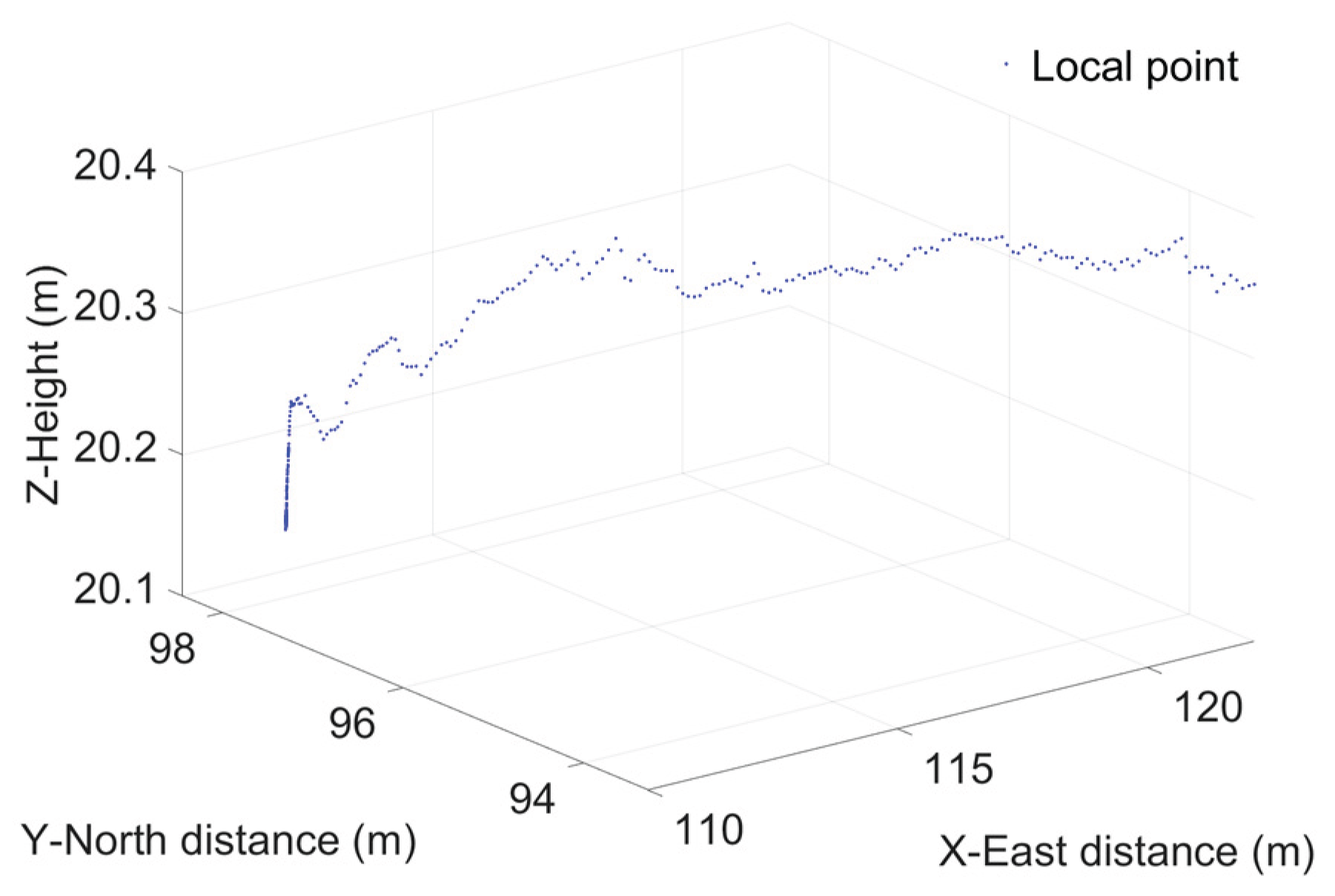
During paddy field operation trials, data on the hard bottom layer contour and agricultural machinery attitude were extracted during the process of machinery becoming stuck due to hard bottom layer depression. To analyze the complete process of becoming stuck, data from 15 seconds before and after the incident were extracted for analysis. The surface points of the extracted hard bottom layer contour are shown in
Figure 24.
Referring to the correlation analysis results in
Section 3.2.1, under unmanned operation conditions, the positional deviation of agricultural machinery exhibits extremely significant correlations with both the hard-bottom layer height and the local roughness of the hard-bottom layer contour surface. This section analyzes the hard-bottom layer height and local roughness across 300 data sets collected before and after vehicle entrapment. The relationship between hard-bottom layer height and local roughness changes during the 15 seconds preceding and following entrapment is illustrated in
Figure 25.
To visually illustrate the changes in the hard bottom layer contour and surface roughness before and after vehicle entrapment, contour points of the hard bottom layer and local contour points were plotted at 0.1-second intervals over a 30-second period before and after entrapment. Fitted straight lines were then calculated for the local roughness, as shown in
Figure 26.
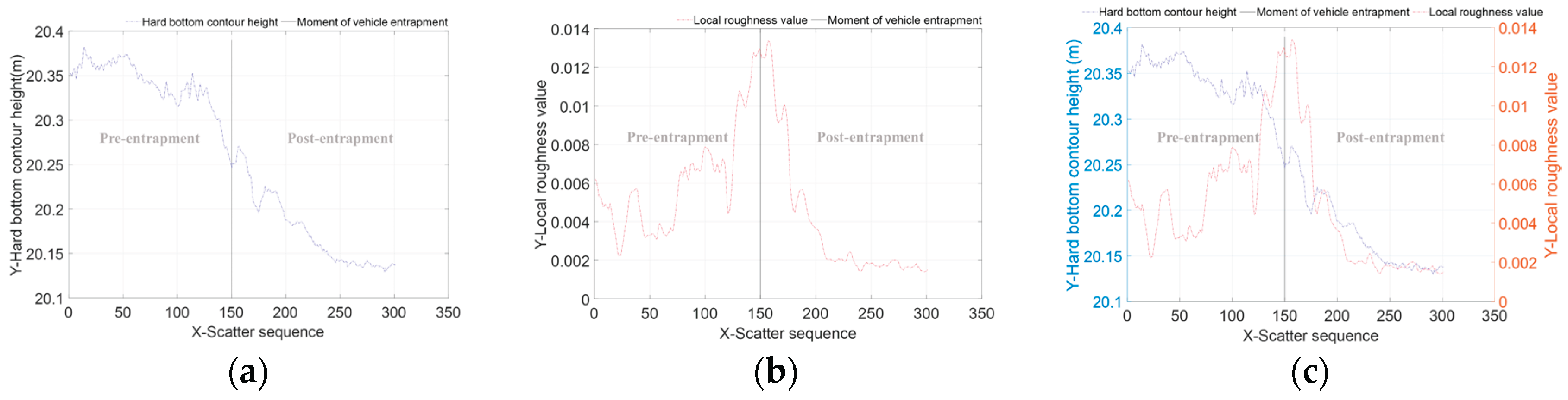
As shown in
Figure 25 and
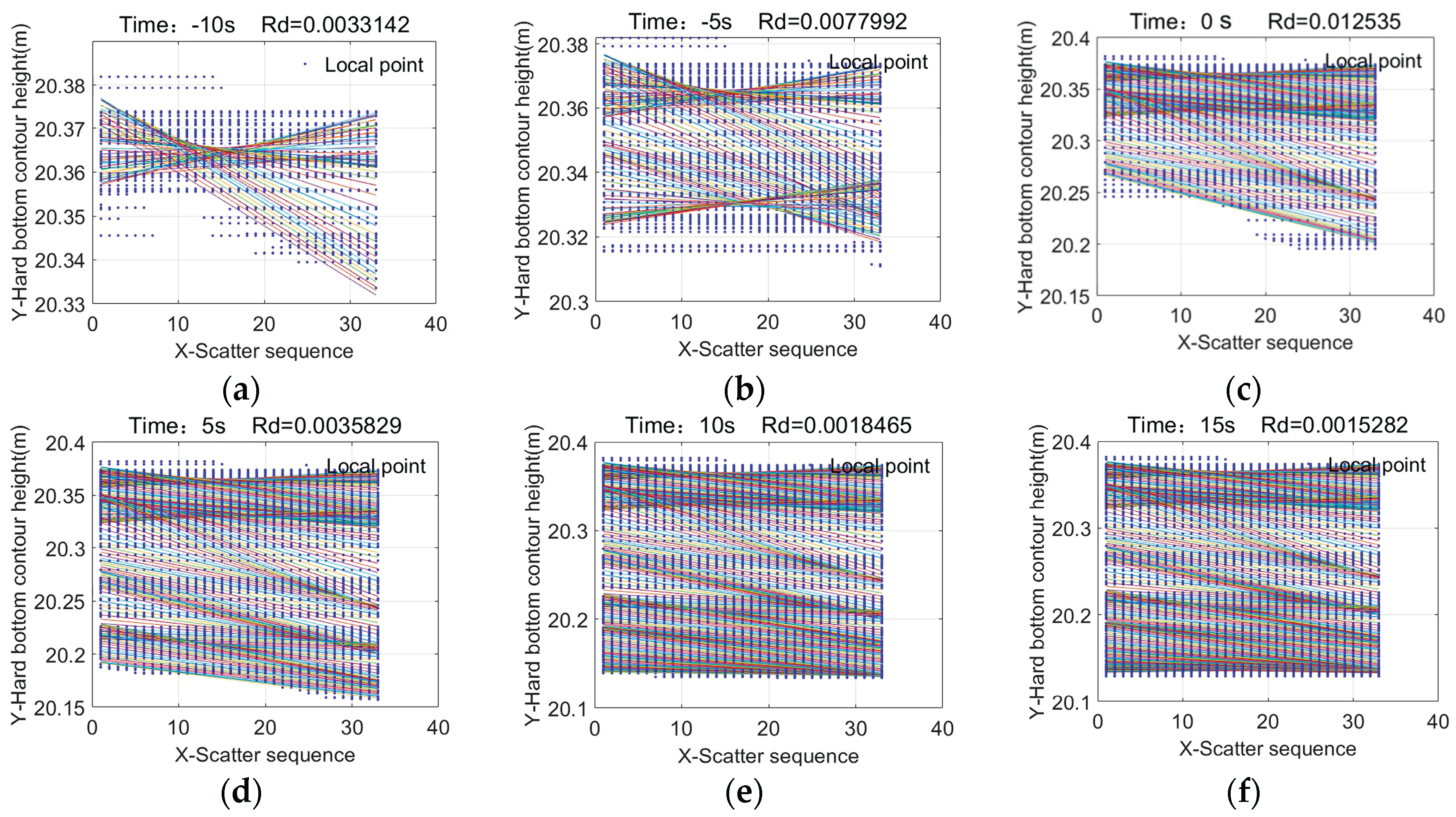
Figure 26, during the normal operation segment (-15 s to -5 s) in paddy fields, the average elevation of the hard bottom layer contour tends to stabilize. Adjacent local contour fitting lines exhibit an alternating pattern, with the local roughness of the hard bottom layer contour fluctuating between 0.002 and 0.008. During the pre- and post-vehicle- trapping segments (-5 s to 5 s), as the vehicle approaches a low-lying area, the hard bottom contour elevation drops sharply. Adjacent local contour fitting lines exhibit a rapid downward shift, and the local roughness of the hard bottom contour increases dramatically. At the moment of initial trapping (“0 s”), the local roughness value peaks at 0.0125. During the post- trapping phase (5 s–15 s), The slip ratio between the agricultural machinery wheels and the hard base layer increases to pure sliding. The contour elevation of the hard base layer decreases gradually, and the adjacent local contour fitting lines exhibit a slow downward shift. The local roughness of the hard base layer contour decreases sharply, with the local roughness value dropping to 0.0014, approaching the 0.0011 value observed during idle parking.
Based on changes in contour elevation and local roughness, construct segmented discriminant functions for pre- and post-wheel- trapping states. Let the agricultural machinery's motion state at time
be
, the hard-bottom layer elevation change rate be
, and the local roughness be
. the local roughness change rate is
, the upper threshold for roughness is
, and the contour height change rate threshold is
. Then:
Based on
Figure 25 and
Figure 26 and the segmented vehicle-trapping discrimination function (24), it is evident that in typical vehicle- trapping scenarios on paddy fields, when a decline in the hard-bottom contour is detected alongside a sharp increase in local roughness exceeding the upper threshold of 0.01, the agricultural machinery faces a risk of trapping. When a decrease in the hard-bottom contour is detected alongside a decrease in local roughness values, it indicates that the agricultural machinery has become trapped. This provides a basis for predicting trapping incidents caused by hard-bottom depressions in paddy fields and for designing post-trapping recovery strategies.
4. Discussion
This study investigates the influence patterns of hard-bottom layer contours on the position and attitude changes of agricultural machinery. By integrating GNSS and AHRS sensors, a system for collecting position/attitude and hard-bottom layer information was established, revealing the mechanism by which typical paddy field terrain features affect the attitude response of unmanned agricultural machinery during operation. The findings indicate that the geometric characteristics and local roughness parameters of the hard bottom contour significantly influence the heading stability, lateral stability, attitude changes, and trapping risk of agricultural machinery. This research provides crucial theoretical and technical support for path planning and driving control in unmanned precision agricultural operations.
The proposed method for acquiring hard-bottom contour data and integrating pose information achieves the acquisition and fusion of motion state data from multiple key points (antenna, wheel bottom, rear axle center) by mounting GNSS and AHRS on the power chassis of a rice transplanter. This provides a foundation for dynamic analysis of agricultural machinery's attitude response characteristics. The study reveals the influence patterns of ridge height and local roughness variations on heading deviation and attitude response, providing a basis for speed control and path tracking of agricultural machinery in complex terrain. Notably, the finding that a 10 cm ridge causes 2–3 times greater heading deviation than a 5 cm ridge indicates terrain undulations significantly impact path accuracy in autonomous agricultural machinery. Large-diameter tires effectively mitigate this effect, offering a mechanical design approach to enhance driving stability.
Additionally, after correcting the positional deviations of the rear axle center and bottom of the wheel center using the attitude correction algorithm, the lateral deviation accuracy improved by approximately 40% compared to antenna measurements. This demonstrates the feasibility and necessity of the attitude fusion correction algorithm for enhancing positioning accuracy. These findings provide practical guidance for optimizing attitude solution models and improving multi-sensor fusion algorithms in unmanned agricultural machinery.
The results of the vehicle trapping test indicate that when the hard-bottom contour drops sharply within a short time and the roughness increases to 0.01, agricultural machinery is prone to trapping. This validates that the hard-bottom contour parameters can serve as key indicators for predicting trapping risk and establishes a segmented discrimination function for trapping states. This provides criteria for establishing pre-trapping warnings and escape strategies during unmanned operations. By integrating real-time hard-bottom contour change rate and roughness threshold parameters into the autonomous control system, adaptive adjustments to speed and posture response strategies can be achieved during operations, thereby enhancing operational safety and continuity.
However, since the experimental platform utilizes a rice transplanting power chassis, the stiffness and vibration characteristics of the sensor mounting location exert a certain influence on measurement accuracy under bumpy terrain conditions. Future improvements in data stability can be achieved through structural optimization and high-precision attitude fusion algorithms. Furthermore, the hard-bottom contour sampling range and temporal resolution in this study remain confined to offline processing. Integrating real-time data streams for dynamic modeling and feature recognition could enable online assessment and adaptive control of agricultural machinery operation status, representing a key direction for future research.
In summary, the proposed method for analyzing the influence of hard bottom contours on the position and attitude changes of agricultural machinery not only provides a theoretical basis for revealing the relationship between terrain and the dynamic response of agricultural machinery, but also offers technical references for unmanned precision operation path planning, vehicle entrapment early warning, and agricultural machinery structural optimization. This holds significant importance for advancing the autonomous perception and intelligent decision-making capabilities of smart agricultural machinery systems.
5. Conclusions
To reveal the influence patterns of hard bottom contour on changes in the position and attitude of agricultural machinery during operation, this study utilizes a rice transplanter chassis equipped with GNSS and AHRS to establish a platform for synchronous acquisition of agricultural machinery position/attitude data and hard bottom contour information. It proposes a method for analyzing the correlation between operational movement states and contour feature parameters, revealing the influence patterns of hard bottom contour characteristics on agricultural machinery attitude response and the mechanism of vehicle entrapment. Key findings include:
(1) A platform for acquiring agricultural machinery pose information and hard-bottom contour features was established. Through multi-sensor fusion of GNSS and AHRS, continuous collection of agricultural machinery operating status and parameters such as hard-bottom elevation and local roughness was achieved, ensuring high-precision data acquisition and temporal consistency. A pose response model for key components of agricultural machinery was constructed.
(2) A correlation analysis method was established between the movement state of agricultural machinery and the contour features of the hard bottom layer. Results indicate that the lateral deviation and heading deviation of the machinery exhibit extremely significant correlations with the Z-axis elevation difference between the bottom of left and right wheels and the local roughness of the hard bottom layer contour, respectively. Changes in ridge height significantly affect the machinery's heading. A mathematical model for agricultural machinery heading response based on hard-bottom elevation differences and wheel diameter was constructed, achieving a coefficient of determination R² of 0.92. Field tests confirmed that when ridge height increased from 5 cm to 10 cm, the magnitude of heading deviation was 2–3 times greater than at the lower height, validating both the significant impact of terrain undulations on driving stability and the reliability of the model.
(3) The attitude response and correction characteristics of wheeled agricultural machinery during ridge crossing were elucidated. Under typical ridge-crossing conditions, large-diameter wheels effectively mitigate heading rate changes caused by terrain disturbances, demonstrating superior driving stability. The front axle suspension system reduces the impact of hard-surface excitation, while the machine's roll attitude is primarily influenced by terrain features encountered by the rear wheels. A theoretical model was developed to predict antenna position deviation relative to the horizontal plane during machine roll. Experiments demonstrate that after attitude correction, lateral deviations at the rear axle center and bottom of the wheel center remain within 0.0108–0.0112 m, improving positioning accuracy by 40.7% and 39.0% respectively compared to direct antenna measurements, validating the effectiveness of the attitude compensation and motion correction models.
(4) A vehicle bogging-in identification and early warning criterion based on dynamic changes in the hard-bottom contour was proposed. In typical bogging-in tests, when a rapid decrease in hard-bottom elevation accompanied by a sharp increase in local roughness exceeding 0.01 is detected within a 5-second timeframe, the agricultural machinery is deemed to be in an imminent bogging-in state. If roughness simultaneously decreases, it indicates that trapping has already occurred. This reveals the dynamic evolution patterns of hard-bottom elevation and local roughness before and after trapping, establishing a segmented discrimination function for agricultural machinery trapping status. This provides a theoretical basis for 5-second advance warning and escape control strategies before typical trapping events.
This study investigates the influence of hard bottom contours on the position and attitude changes of agricultural machinery during movement. It establishes quantitative relationships among hard bottom contour characteristics, agricultural machinery attitude responses, and vehicle entrapment states. The findings provide theoretical foundations and technical support for intelligent path tracking control, chassis structure optimization, and unmanned precision operations in agricultural machinery. This research holds significant importance for enhancing the intelligence level and operational efficiency of paddy field machinery.
Author Contributions
Conceptualization, T.T., L.H., X.L., and J.H.; methodology, T.T., L.H., X.L., and J.H.; software, T.T., P.W., P.H., R.Z., and G.C.; validation, T.T., Z.M., D.F., and M.Y.; formal analysis, T.T.; investigation, T.T. and X.D.; resources, T.T., L.H., X.L., J.H., and P.W.; data curation, T.T., L.H., and J.H.; writing—original draft preparation, T.T.; writing—review and editing, T.T., L.H., X.L., and J.H.; visualization, T.T., L.H., P.W., X.D., and J.M.; supervision, L.H., X.L., and J.H.; project administration, X.L.; funding acquisition, T.T., and L.H., and J.H.. All authors have read and agreed to the published version of the manuscript.
Funding
This research was funded by the China Postdoctoral Science Foundation (Grant No. 2024M750955), the National Natural Science Foundation of China (32472016, 32071913), the Postdoctoral Fellowship Pro-gram (Grade C) of China Postdoctoral Science Foundation (Grant No. GZC20230855) and the Lingnan Modern Agricultural Science and Technology Laboratory Independent Research Project (Grant No. NT2025006).
Data Availability Statement
The data that supports this study will be shared upon reasonable request to the corresponding author.
Acknowledgments
We would like to thank our partners of the Zengcheng Teaching Base of South China Agricultural University for their help and support in field management and machine maintenance.
Conflicts of Interest
The authors declare no conflicts of interest.
References
- Nawaz, A.; Rehman, A. U.; Rehman, A.; Ahmad, S.; Siddique, K. H. M.; Farooq, M., Increasing sustainability for rice production systems. Journal of Cereal Science 2022, 103, 103400. [CrossRef]
- Seck, P. A.; Diagne, A.; Mohanty, S.; Wopereis, M. C. S., Crops that feed the world 7: Rice. Food Security 2012, 4, (1), 7-24. [CrossRef]
- Kuenzer, C.; Knauer, K., Remote sensing of rice crop areas. International Journal of Remote Sensing 2013, 34, (6), 2101-2139. [CrossRef]
- Xin, F.; Xiao, X.; Dong, J.; Zhang, G.; Zhang, Y.; Wu, X.; Li, X.; Zou, Z.; Ma, J.; Du, G.; Doughty, R. B.; Zhao, B.; Li, B., Large increases of paddy rice area, gross primary production, and grain production in Northeast China during 2000–2017. Science of The Total Environment 2020, 711, 135183. [CrossRef]
- He, J.; Hu, L.; Wang, P.; Liu, Y.; Man, Z.; Tu, T.; Yang, L.; Li, Y.; Yi, Y.; Li, W.; Luo, X., Path tracking control method and performance test based on agricultural machinery pose correction. Computers and Electronics in Agriculture 2022, 200, 107185. [CrossRef]
- Hu, L.; Luo, X.; Lin, C.; Yang, W.; Xu, Y.; Li, Q., Development of 1PJ-4.0 laser leveler installed on a wheeled tractor for paddy field. Nongye Jixie Xuebao= Transactions of the Chinese Society for Agricultural Machinery 2014, 45, (4), 146-151.
- Luo, X.; Hu, L.; He, J.; Zhang, Z.; Zhou, Z.; Zhang, W.; Liao, J.; Huang, P., Key technologies and practice of unmanned farm in China. Transactions of the Chinese Society of Agricultural Engineering 2024, 40, (1), 1-16.
- 9Tu, T.; He, J.; Luo, X.; Hu, L.; Wang, P.; Chen, G.; Tian, L.; Feng, D.; Wang, Z.; Man, Z.; Li, W.; Wei, Z.; Peng, J.; Yi, Y.; Wu, P., Methods and experiments for collecting information and constructing models of bottom-layer contours in paddy fields. Computers and Electronics in Agriculture 2023, 207, 107719. [CrossRef]
- Luo, X.; Liao, J.; Hu, L.; Zang, Y.; Zhou, Z., Improving agricultural mechanization level to promote agricultural sustainable development. Transactions of the Chinese Society of Agricultural Engineering 2016, 32, (1), 1-11.
- Luo, X.; Liao, J.; Hu, L.; Zhou, Z.; Zhigang, Z.; Zang, Y.; Wang, P.; He, J., Research progress of intelligent agricultural machinery and practice of unmanned farm in China. Journal of South China Agricultural University 2021, 42, (6), 8-17.
- Bekker, M. G., Introduction to Terrain–Vehicle Systems. University of Michigan Press: Ann Arbor, MI, USA, 1969.
- Wong, J. Y., Theory of Ground Vehicles (4th Edition). Wiley: Hoboken, NJ, USA, 2010.
- Jia, Z.; Smith, W.; Peng, H., Terramechanics-based wheel–terrain interaction model and its applications to off-road wheeled mobile robots. Robotica 2012, 30, (3), 491-503. [CrossRef]
- Misaghi, S.; Tirado, C.; Nazarian, S.; Carrasco, C., Impact of pavement roughness and suspension systems on vehicle dynamic loads on flexible pavements. Transportation engineering (Oxford) 2021, 3, 100045. [CrossRef]
- Guo, Z.; Li, A.; Feng, J.; Zheng, Y.; Qin, D.; Ge, S., Influence of the driving environment on the dynamic characteristics of a DCT vehicle starting considering the longitudinal and vertical coupling model. Scientific Reports 2024, 14, (1), 29698. [CrossRef]
- Inotsume, H.; Kubota, T., Terrain traversability prediction for off-road vehicles based on multi-source transfer learning. ROBOMECH Journal 2022, 9, (1), 6. [CrossRef]
- Golanbari, B.; Mardani, A.; Hosainpour, A.; Taghavifar, H., Predicting terrain deformation patterns in off-road vehicle-soil interactions using TRR algorithm. Journal of terramechanics 2025, 117, 101021. [CrossRef]
- Tu, T.; Hu, L.; Luo, X.; He, J.; Wang, P.; Tian, L.; Chen, G.; Man, Z.; Feng, D.; Cen, W.; Li, M.; Liu, Y.; Hou, K.; Zi, L.; Yue, M.; Li, Y., Method and Experiment for Quantifying Local Features of Hard Bottom Contours When Driving Intelligent Farm Machinery in Paddy Fields. Agronomy 2023, 13, (7), 1949. [CrossRef]
- Tu, T.; Luo, X.; Hu, L.; Chung, S.; He, J.; Zhao, R.; Wang, P.; Chen, G.; Feng, D.; Yue, M.; Man, Z.; Karim, M. R.; Ruan, Q.; Jiang, X.; Wu, P., Methods and experiments for analysing hard-bottom layer changes and monitoring wheel sink depth in paddy fields. Computers and Electronics in Agriculture 2025, 238, 110760. [CrossRef]
- Lenain, R.; Thuilot, B.; Cariou, C.; Martinet, P., High accuracy path tracking for vehicles in presence of sliding: Application to farm vehicle automatic guidance for agricultural tasks. Autonomous Robots 2006, 21, (1), 79-97. [CrossRef]
- Liu, Z.; Zhang, Z.; Luo, X.; Wang, H.; Huang, P.; Zhang, J., Design of automatic navigation operation system for Lovol ZP9500 high clearance boom sprayer based on GNSS. Transactions of the Chinese Society of Agricultural Engineering 2018, 34, (1), 15-21.
- Anderson, R. A., Using GPS for model based estimation of critical vehicle states and parameters. In 2004.
- Bevly, D. M.; Gerdes, J. C.; Wilson, C.; Zhang, G., The use of GPS based velocity measurements for improved vehicle state estimation. In 2000; pp 2538-2542.
- Ryu, J.; Gerdes, J. C., Integrating inertial sensors with global positioning system (GPS) for vehicle dynamics control. J. Dyn. Sys., Meas., Control 2004, 126, (2), 243-254. [CrossRef]
- Hiraoka, T.; Nishihara, O.; Kumamoto, H., Automatic path-tracking controller of a four-wheel steering vehicle. Vehicle System Dynamics 2009, 47, (10), 1205-1227. [CrossRef]
- Lucet, E.; Lenain, R.; Grand, C., Dynamic path tracking control of a vehicle on slippery terrain. Control Engineering Practice 2015, 42, 60-73. [CrossRef]
- Lenain, R.; Thuilot, B.; Cariou, C.; Martinet, P., Mixed kinematic and dynamic sideslip angle observer for accurate control of fast off-road mobile robots. Journal of Field Robotics 2010, 27, (2), 181-196. [CrossRef]
- Zhou, J.; Xu, J.; Wang, Y.; Liang, Y., Development of Paddy Field Rotary-leveling Machine Based on GNSS. Transactions of the Chinese Society for Agricultural Machinery 2020, 51, (4), 38-43.
- Xin, F.; Xiao, X.; Dong, J.; Zhang, G.; Zhang, Y.; Wu, X.; Li, X.; Zou, Z.; Ma, J.; Du, G.; Doughty, R. B.; Zhao, B.; Li, B., Large increases of paddy rice area, gross primary production, and grain production in Northeast China during 2000–2017. Science of The Total Environment 2020, 711, 135183. [CrossRef]
Figure 1.
Platform for collecting agricultural machinery pose information and bottom layer contour data.
Figure 1.
Platform for collecting agricultural machinery pose information and bottom layer contour data.
Figure 2.
Schematic diagram showing the relationship between the local cutting plane coordinate system {t}, the vehicle body coordinate system {b}, and the position of the rear bottom of the wheel of the vehicle body.
Figure 2.
Schematic diagram showing the relationship between the local cutting plane coordinate system {t}, the vehicle body coordinate system {b}, and the position of the rear bottom of the wheel of the vehicle body.
Figure 3.
Left View During Vehicle Pitching.
Figure 3.
Left View During Vehicle Pitching.
Figure 4.
Full-field wheel track pattern.
Figure 4.
Full-field wheel track pattern.
Figure 5.
Hard bottom layer contour curve: (a) Segmented trajectory; (b) 3D spline curve fitting.
Figure 5.
Hard bottom layer contour curve: (a) Segmented trajectory; (b) 3D spline curve fitting.
Figure 6.
Relationship between hard bottom layer, local fitted line segments, and height of contour points relative to the fitted straight line.
Figure 6.
Relationship between hard bottom layer, local fitted line segments, and height of contour points relative to the fitted straight line.
Figure 7.
Schematic diagram of lateral deviation and heading deviation in agricultural machinery. Note: In the figure, represents the target heading angle, denotes the heading angle deviation, and indicates the lateral position deviation. The target navigation line is formed by points and , with serving as the target navigation point.
Figure 8.
Schematic diagram of a typical vehicle entrapment process.
Figure 8.
Schematic diagram of a typical vehicle entrapment process.
Figure 9.
Digital model of hard bottom layer in fields where vehicle trapping occurred.
Figure 9.
Digital model of hard bottom layer in fields where vehicle trapping occurred.
Figure 10.
Planned working path and field site for unmanned direct seeding machine: (a) Planned working path; (b) Field site.
Figure 10.
Planned working path and field site for unmanned direct seeding machine: (a) Planned working path; (b) Field site.
Figure 11.
Schematic diagram of hard road surface testing.
Figure 11.
Schematic diagram of hard road surface testing.
Figure 12.
Schematic diagram of hard road surface test: (a) Driving over a 5cm-high trapezoidal ridge; (b) Driving over a 10cm-high trapezoidal ridge.
Figure 12.
Schematic diagram of hard road surface test: (a) Driving over a 5cm-high trapezoidal ridge; (b) Driving over a 10cm-high trapezoidal ridge.
Figure 13.
Trajectory curve and heading change rate of agricultural machinery: (a) Trajectory of agricultural machinery traversing ridge platforms; (b) Heading changes during agricultural machinery traversal of ridge platforms.
Figure 13.
Trajectory curve and heading change rate of agricultural machinery: (a) Trajectory of agricultural machinery traversing ridge platforms; (b) Heading changes during agricultural machinery traversal of ridge platforms.
Figure 14.
Heading and heading change rate during the process of agricultural machinery traversing ridge platforms.
Figure 14.
Heading and heading change rate during the process of agricultural machinery traversing ridge platforms.
Figure 15.
Comparison between measured and model-predicted heading change values.
Figure 15.
Comparison between measured and model-predicted heading change values.
Figure 16.
Dynamic process of height difference between left and right rear axles and its rate of change.
Figure 16.
Dynamic process of height difference between left and right rear axles and its rate of change.
Figure 17.
Positioning antenna trajectory and planned heading.
Figure 17.
Positioning antenna trajectory and planned heading.
Figure 18.
Primary positioning antenna, rear axle center, and wheel track.
Figure 18.
Primary positioning antenna, rear axle center, and wheel track.
Figure 19.
Antenna trajectory and its lateral deviation: (a) Antenna trajectory; (b) Antenna lateral deviation.
Figure 19.
Antenna trajectory and its lateral deviation: (a) Antenna trajectory; (b) Antenna lateral deviation.
Figure 20.
Center trajectory of the rear axle on agricultural machinery and its lateral deviation: (a) Center trajectory of agricultural machinery rear axle; (b) Lateral deviation of agricultural machinery rear axle center.
Figure 20.
Center trajectory of the rear axle on agricultural machinery and its lateral deviation: (a) Center trajectory of agricultural machinery rear axle; (b) Lateral deviation of agricultural machinery rear axle center.
Figure 21.
Center trajectory of the line connecting the left and right wheel bottoms and its lateral deviation; (a) Center trajectory of wheelbase connection lines; (b) Lateral deviation of wheelbase connection line center.
Figure 21.
Center trajectory of the line connecting the left and right wheel bottoms and its lateral deviation; (a) Center trajectory of wheelbase connection lines; (b) Lateral deviation of wheelbase connection line center.
Figure 22.
Comparison of standard deviations for lateral deviations across different sections.
Figure 22.
Comparison of standard deviations for lateral deviations across different sections.
Figure 23.
Schematic diagram showing antenna position deviation when the agricultural machinery rolls compared to the horizontal position.
Figure 23.
Schematic diagram showing antenna position deviation when the agricultural machinery rolls compared to the horizontal position.
Figure 24.
Surface points of the hard bottom layer 15 seconds before and after vehicle entrapment.
Figure 24.
Surface points of the hard bottom layer 15 seconds before and after vehicle entrapment.
Figure 25.
Relationship between hard substrate height and local roughness change before and after 30 s trapping: (a) Height variation contour of the hard bottom layer contour; (b) Local roughness variation contour of the hard bottom layer contour; (c) Hard bottom layer contour height variation and local roughness variation curves.
Figure 26.
Changes in hard substrate height and local roughness from 15 s before to 15 s after trapping: (a) -15 s~-10 s; (b) -10 s~-5 s; (c) -5 s~0 s; (d) 0 s~5 s; (e) 5s~10 s; (f) 10 s~15 s.
Figure 26.
Changes in hard substrate height and local roughness from 15 s before to 15 s after trapping: (a) -15 s~-10 s; (b) -10 s~-5 s; (c) -5 s~0 s; (d) 0 s~5 s; (e) 5s~10 s; (f) 10 s~15 s.
Table 1.
Correlation analysis between hard bottom layer contour characteristics and agricultural machinery motion parameters.
Table 1.
Correlation analysis between hard bottom layer contour characteristics and agricultural machinery motion parameters.
| Variable |
Lateral deviation (m) |
|
Heading deviation (°) |
|
| |
Pearson correlation |
Sig. (2-tailed) |
Pearson correlation |
Sig. (2-tailed) |
| Hardpan feature parameters |
|
|
|
|
| X-coordinate of left wheel–hardpan contact point (m) |
−.042* |
0.021 |
−.101** |
0.000 |
| Y-coordinate of left wheel–hardpan contact point (m) |
.040* |
0.026 |
.101** |
0.000 |
| Z-coordinate of left wheel–hardpan contact point (m) |
.156** |
0.000 |
.056** |
0.002 |
| X-coordinate of right wheel–hardpan contact point (m) |
−.042* |
0.020 |
−.102** |
0.000 |
| Y-coordinate of right wheel–hardpan contact point (m) |
.040* |
0.025 |
.102** |
0.000 |
| Z-coordinate of right wheel–hardpan contact point (m) |
.056** |
0.002 |
−0.002 |
0.917 |
| Height difference between left and right wheel contact points (m) |
.142** |
0.000 |
.075** |
0.000 |
| Local roughness of contour |
.094** |
0.000 |
−.118** |
0.000 |
| Machinery posture parameters |
|
|
|
|
| Antenna height (m) |
.102** |
0.000 |
.114** |
0.000 |
| Speed (m/s) |
.152** |
0.000 |
−0.027 |
0.129 |
| Heading angle (°) |
−.341** |
0.000 |
−.999** |
0.000 |
| Pitch angle (°) |
.070** |
0.000 |
.151** |
0.000 |
| Roll angle (°) |
.142** |
0.000 |
.075** |
0.000 |
| Left wheel velocity (m/s) |
0.017 |
0.337 |
−0.010 |
0.561 |
| Right wheel velocity (m/s) |
.152** |
0.000 |
−0.019 |
0.289 |
| Velocity difference between left and right wheels (m/s) |
−.377** |
0.000 |
0.024 |
0.180 |
| Left wheel acceleration (m/s²) |
−0.002 |
0.913 |
−0.013 |
0.458 |
| Right wheel acceleration (m/s²) |
0.006 |
0.732 |
0.012 |
0.493 |
| Acceleration difference between left and right wheels (m/s²) |
−.041* |
0.021 |
−.131** |
0.000 |
| Center velocity (m/s) |
.088** |
0.000 |
−0.019 |
0.282 |
| Center acceleration (m/s²) |
0.002 |
0.892 |
0.000 |
0.995 |
Table 2.
Heading variation during ridge crossing.
Table 2.
Heading variation during ridge crossing.
| Stage ID |
Description |
Heading (°) |
Heading Change (°) |
Maximum heading change rate (°/s) |
| A-1 |
Front wheel crossing the first 5 cm ridge |
-89.15 |
0.85 |
6.694 |
| B-1 |
Rear wheel crossing the first 5 cm ridge |
-88.66 |
0.49 |
6.039 |
| A-2 |
Front wheel crossing the second 5 cm ridge |
-87.85 |
0.81 |
8.259 |
| B-2 |
Rear wheel crossing the second 5 cm ridge |
-87.37 |
0.48 |
7.023 |
| C-1 |
Front wheel crossing the first 10 cm ridge |
-85.06 |
2.31 |
13.57 |
| D-1 |
Rear wheel crossing the first 10 cm ridge |
-83.72 |
1.34 |
10.49 |
| C-2 |
Front wheel crossing the second 10 cm ridge |
-81.32 |
2.4 |
12.88 |
| D-2 |
Rear wheel crossing the second 10 cm ridge |
-80.15 |
1.17 |
7.552 |
Table 3.
Comparison between actual and predicted heading change values.
Table 3.
Comparison between actual and predicted heading change values.
| Sample No. |
Ridge
height (m) |
Wheel diameter (m) |
Actual heading change (°) |
Predicted heading change(°) |
| 1 |
0.05 |
0.65 |
0.85 |
1.02 |
| 2 |
0.05 |
0.95 |
0.49 |
0.3 |
| 3 |
0.05 |
0.65 |
0.81 |
1.02 |
| 4 |
0.05 |
0.95 |
0.48 |
0.3 |
| 5 |
0.1 |
0.65 |
2.31 |
2.17 |
| 6 |
0.1 |
0.95 |
1.34 |
1.44 |
| 7 |
0.1 |
0.65 |
2.4 |
2.17 |
| 8 |
0.1 |
0.95 |
1.17 |
1.44 |
Table 4.
Standard deviations of lateral deviations for different sections.
Table 4.
Standard deviations of lateral deviations for different sections.
| Section |
Antenna lateral deviation SD (m) |
Rear axle center lateral deviation SD (m) |
Rear wheel midpoint lateral deviation SD (m) |
| 5 cm Ridge |
0.0143 |
0.0109 |
0.0108 |
| 10 cm Ridge |
0.0200 |
0.0107 |
0.0112 |
| Entire section (5 cm + 10 cm) |
0.0182 |
0.0108 |
0.0111 |
|
Disclaimer/Publisher’s Note: The statements, opinions and data contained in all publications are solely those of the individual author(s) and contributor(s) and not of MDPI and/or the editor(s). MDPI and/or the editor(s) disclaim responsibility for any injury to people or property resulting from any ideas, methods, instructions or products referred to in the content. |
© 2025 by the authors. Licensee MDPI, Basel, Switzerland. This article is an open access article distributed under the terms and conditions of the Creative Commons Attribution (CC BY) license (http://creativecommons.org/licenses/by/4.0/).