
Submitted:
24 November 2025
Posted:
25 November 2025
You are already at the latest version
Abstract
Quality assurance in aluminum die casting is critical, as internal defects—such as porosity—can compromise structural integrity and significantly reduce component service life. In the cost-sensitive manufacturing environment of Germany, early and automated rejection of defective parts is essential to minimize scrap, rework, and energy waste. This study investigates the feasibility and performance of deep learning for automated defect detection in industrial X-ray images of two series-production aluminum die-cast components. A systematic methodology was employed: first, candidate object-detection frameworks (YOLOv5 vs. Faster R-CNN) were evaluated under real-time constraints (< 2 s per image) on standard industrial hardware; subsequently, position-specific and single global models were trained on annotated datasets. A systematic hyperparameter study—focusing on input resolution, learning rate, and loss weights—was conducted to optimize accuracy and robustness. The best-performing models achieved F1-scores up to 0.87, with position-specific models outperforming the single global model on average. The approach was validated under real production conditions at Hengst SE (Nordwalde), demonstrating practical feasibility, strong acceptance among quality professionals, and significant potential to accelerate inspections and standardize decision-making. The results confirm that deep learning is a viable alternative to rule-based image processing and holds substantial promise for automating X-ray inspection workflows in aluminum die casting—contributing to both operational efficiency and sustainability goals.
Keywords:
aluminum die casting
; X-ray inspection
; porosity defects
; deep learning
; industrial inspection
; quality assurance
; case study TRL-Level 7
1. Introduction
Quality assurance is critical in aluminum die casting because internal porosity—such as gas and shrinkage pores—can compromise structural integrity and significantly shorten component lifetime. X-ray inspection is therefore a cornerstone of non-destructive testing (NDT), enabling the identification of defective parts before machining or assembly, thereby preventing costly rework, recalls, and downstream failures.
Currently, inspection remains largely manual. Visual judgment is highly dependent on operator experience and fatigue, making subtle porosity patterns easy to overlook. This variability leads to inconsistent decision-making, increased scrap rates, and higher production costs. Recent advances in deep learning (DL) offer a promising solution: convolutional neural networks (CNNs) and modern one-stage object detectors achieve high accuracy in industrial imaging with low inference latency. State-of-the-art studies report detection accuracies of up to 95.9% on specific datasets, with multiple works demonstrating that DL-based approaches outperform classical image processing methods in complex defect scenarios [3,4,5].
Economic pressures further underscore the need for robust and efficient inspection. The global market for X-ray inspection systems is expanding rapidly, while energy prices remain high for German industry—amplifying the financial and environmental cost of scrap in energy-intensive die casting processes. Reducing false negatives and rework not only improves profitability but also contributes directly to sustainability goals. For context, the market for X-ray inspection systems is estimated at USD 2.50 billion in 2024 and projected to reach USD 3.85 billion by 2032 [6]; in Germany, electricity prices for industrial consumers averaged approximately 0.178 €/kWh in 2025 [10].
This study develops and evaluates a deep learning-based object detection system for automated porosity detection in X-ray images of aluminum die-cast components. The solution is specifically tailored to project requirements at Hengst SE, Germany: real-time processing (< 2 s per image) on a standard industrial PC without a discrete GPU, and seamless integration into the existing X-ray inspection workflow. The approach is validated in a real-world industrial case study under actual production conditions, and the methodology and results are detailed in Section 2 and Section 3, respectively.
This study addresses the following research questions:
- (RQ1) Can a one-stage deep learning detector meet real-time constraints (< 2 s) on standard industrial hardware without a discrete GPU?
- (RQ2) How does input resolution affect detection accuracy for small porosity defects in aluminum die-cast X-ray images?
- (RQ3) Does model granularity (position-specific vs. part-level) impact detection performance and generalization in real-world production conditions?
Based on these questions, we formulate the following hypotheses:
- (H1) A one-stage detector (e.g., YOLOv5) will satisfy real-time constraints, while a two-stage detector (e.g., Faster R-CNN) will not.
- (H2) Preserving native image resolution (2016 × 2016) will significantly improve detection accuracy compared to downscaling.
- (H3) Position-specific models will outperform a Part-Level model in localization accuracy, but the Part-Level model may generalize better across inspection positions.
The remainder of this paper is structured as follows: Section 2 details the industrial context, dataset curation, and methodological framework, including model preselection, hyperparameter optimization, and evaluation protocol. Section 3 presents the quantitative and qualitative results, including runtime performance, F1-scores, and live test outcomes. Section 4 discusses the implications of the findings for industrial practice, limitations, and future work. Finally, Section 5 concludes with practical recommendations for deploying AI in industrial inspection workflows.
2. Methodology: A Four-Stage Framework for Deployable Defect Detection
2.1. Industrial Context and Equipment
The study was conducted in a production X-ray inspection cell at Hengst SE (Nordwalde, Germany). The system comprises an X-Cube Compact X-ray cabinet (maximum tube voltage 225 kV) and the vendor’s inspection software VistaPlusV for image acquisition and operator viewing. Components are mounted in a dedicated production clamping fixture (workholding fixture) that enforces a highly repeatable pose for series inspection. Each part is examined according to predefined routines with a fixed number of inspection positions (views). For every unit under test, the same set of positions is acquired in the same order; images are 2D radiographs (no CT) captured using site-standard exposure recipes.
2.2. Dataset Curation and Annotation
We collected production radiographs for two aluminum die-cast components, hereafter Part A and Part B. Part A is inspected in nine predefined positions (POS1–POS9) with 300 images per position, totaling 2,700 images and 12,960 porosity annotations. Part B is inspected in eighteen positions (POS1–POS18) with 150 images per position, totaling 2,700 images and 27,443 annotations. Images were acquired during regular shifts and exported by VistaPlusV to a network share using a minimal filename scheme PartA_POS<k> or PartB_POS<k>. Invalid images (e.g., misclamping, severe rotation/vertical offset, non-representative machining states) were removed before labeling. Porosity defects were annotated as bounding boxes (single class porosity) using LabelImg [9]; labels store normalized coordinates per image.
For each part and position, the dataset was split into 70% training and 30% validation with no separate test set; the fixed split was reused across all experiments without leakage. Table 1 summarizes the aggregate image and annotation counts per component; Figure 1 and Figure 2 visualize the distribution of annotations per inspection position for Part A and Part B, respectively, with the mean indicated as a dashed reference line.
As shown in Figure 1 and Figure 2, annotation counts vary strongly across inspection positions. For Part A (9 positions), counts range from 477 (POS5) to 1,460 (POS4), with a mean of 894 and a total of 12,960 annotations. For Part B (18 positions), counts range from 346 (POS9) to 2,367 (POS11), with a mean of 1,398 and a total of 27,443 annotations.
2.3. Model Preselection and CPU Runtime Benchmark
To identify a detector family that satisfies the project-specific real-time constraint ( s per image on a CPU-only industrial PC), we conducted a runtime-only preselection comparing a modern one-stage DL detector (YOLOv5) with a two-stage baseline (Faster R-CNN). We used publicly available pretrained weights without additional training or fine-tuning and evaluated end-to-end latency per image. Accuracy was intentionally not compared at this stage; accuracy-focused experiments follow later.
2.3.1. Rationale for Candidate Selection
YOLOv5 and Faster R-CNN represent the two dominant paradigms in object detection (one-stage vs. two-stage) and are widely proven across diverse applications [1,2]. This pairing aligns with deployment constraints: Windows-based CPU-only execution on shop-floor hardware, strict endpoint security, limited admin rights, and packaging as a self-contained executable. YOLOv5 offers low-latency inference and mature export/packaging paths; Faster R-CNN provides a strong accuracy-oriented baseline for runtime comparison. Heavier alternatives (e.g., transformer/anchor-free stacks) were out of scope for the runtime preselection.
2.3.2. Execution Environment and Packaging
Benchmarks ran on the target industrial workstation (CPU-only); inference was wrapped in a lightweight PyQt UI and packaged with PyInstaller as a single-file executable (onefile) to mirror deployment conditions (deterministic dependencies; endpoint security active; no Python environment management). As the benchmark target, the shop-floor hardware and OS are listed in Table 2.
2.3.3. Benchmark Protocol
We measured wall-clock latency per image (batch size 1) on CPU, including model load, preprocessing, inference, postprocessing (NMS), and overlay rendering. To account for warm-up, the first run was recorded separately; subsequent runs were repeated times and summarized by mean, minimum, and maximum. Radiographs were 8-bit grayscale at native resolution 2016×2016, resized per framework to a fixed model input of 640×640 (YOLOv5: square resize; Faster R-CNN: shorter-side resize to 640 with aspect preserved). We report the resulting CPU latencies in Table 3.
2.3.4. Results and Decision
YOLOv5 met the s CPU target after warm-up. Its minimum latency was 1.261 s, mean 1.33 s, and maximum 2.39 s, where the maximum corresponds to the first, initialization run. Faster R-CNN failed the target with higher variability: minimum 3.718 s, mean 5.59 s, and maximum 9.698 s. We therefore selected the one-stage family for full training and tuning.
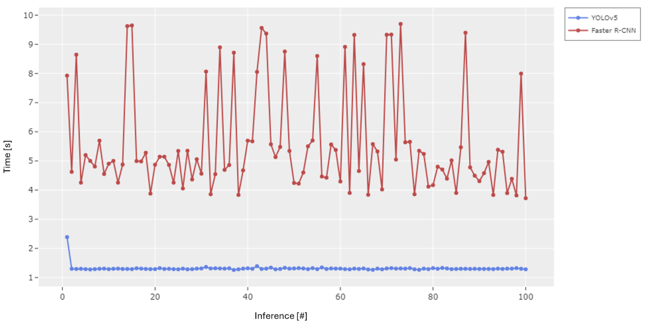
Figure 3.
CPU-only inference latency on the industrial PC over 100 runs (batch size 1). The first-run warm-up outlier is visible for YOLOv5; subsequent runs stabilize well below the 2 s target.
Figure 3.
CPU-only inference latency on the industrial PC over 100 runs (batch size 1). The first-run warm-up outlier is visible for YOLOv5; subsequent runs stabilize well below the 2 s target.
2.4. Baseline Benchmark for YOLO Variant Selection
We compared YOLOv5, YOLOv8, YOLOv9, YOLOv10, and YOLOv11 under identical inputs using the Ultralytics framework. Specifically, we used the dataset of Part A, position 2, with 300 images and 1,100 annotations (single class). Training ran for 250 epochs with default hyperparameters, and performance was measured by the F1-Score.
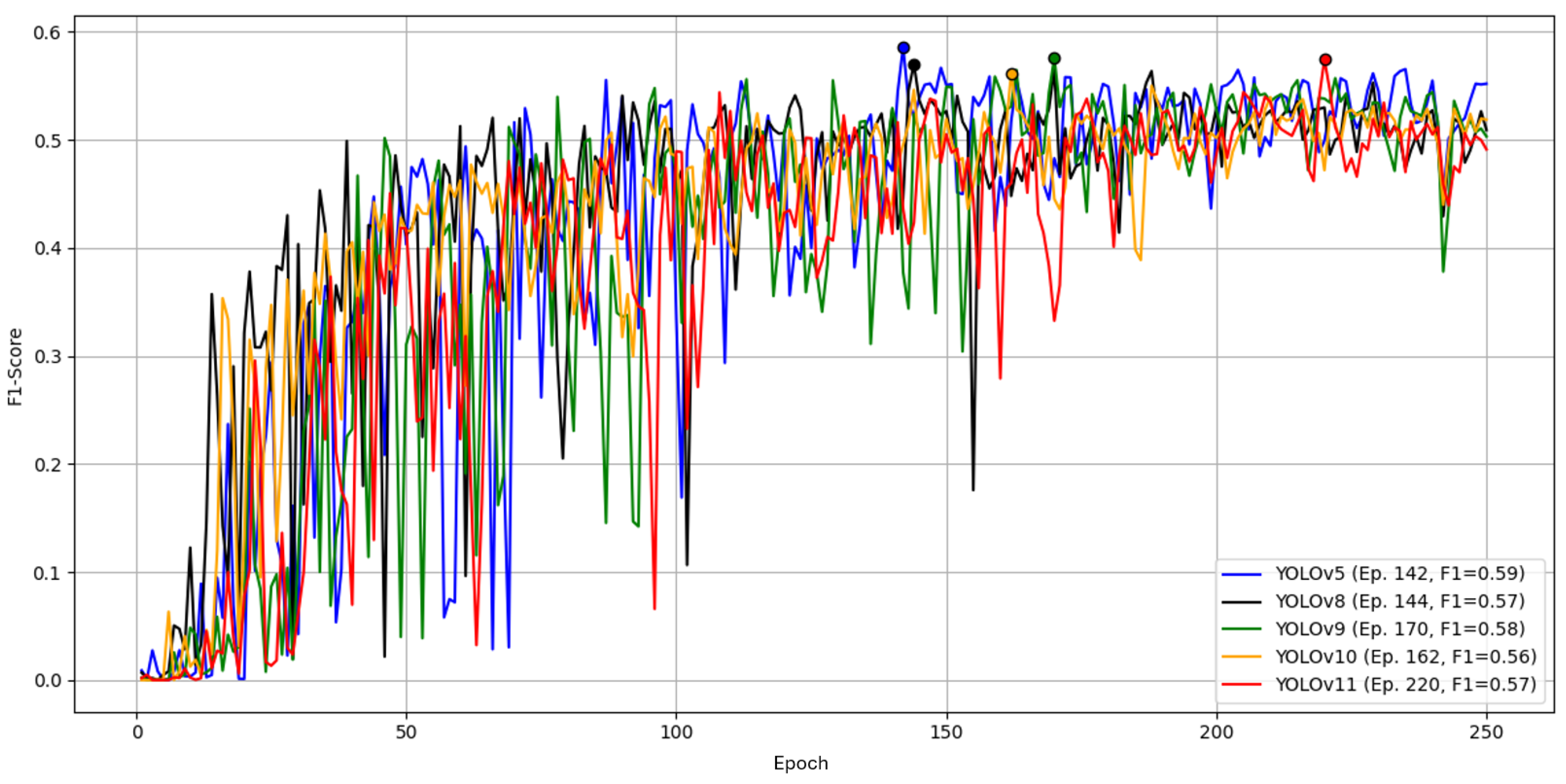
Figure 4.
Comparison of YOLO architectures over 250 epochs by F1 score on the reference dataset. Early oscillations up to ∼100 epochs diminish over time.
Figure 4.
Comparison of YOLO architectures over 250 epochs by F1 score on the reference dataset. Early oscillations up to ∼100 epochs diminish over time.
2.4.1. Results
YOLOv5 achieved the highest peak F1 with at epoch 142, followed by YOLOv9 with at epoch 170. YOLOv8 and YOLOv11 both reached . These differences are small.
As shown in Table 4, YOLOv9 had the shortest total time (18.60 min) but reached its best F1 later (12.45 min). YOLOv5 reached its best F1 fastest (10.20 min) with a similar total time, while YOLOv10 was markedly slower without better F1. Given near-equal peak F1 but faster convergence to the best F1, and low total training time, we select YOLOv5 for subsequent experiments on Parts A and B.
2.5. Hyperparameter Optimization Strategy
Due to long training times and large data volume, hyperparameter optimization was restricted to one position per part and limited to deterministic parameters only to ensure reproducibility, excluding randomness-dependent settings (e.g., initializations, dropout). We optimized on Part A (H183H) position 1 and Part B (H530H) position 6. For each position, we applied a sequential, one-at-a-time procedure: vary a single hyperparameter while keeping others fixed at a baseline, select the best value after several runs, fix it, then proceed to the next hyperparameter until all targeted parameters were adjusted. The resulting per-part parameter set was then transferred to the remaining positions of the same part. In addition, we trained a joint model on a combined dataset of all positions using the same optimal hyperparameters and compared its performance with the average of the position-specific models. The overall procedure is summarized in Figure 5.
2.6. Hyperparameter Optimization on Part A
This section presents an example optimization of YOLOv5 hyperparameters. We start from the YOLOv5 default settings as provided by Ultralytics v8.3.94 (full list in digital Appendix D). By default, training images are resized to pixels. This strongly reduces input size but may hide small casting defects at very high native resolution (). Figure 6 shows identical defects at native resolution and after downscaling, illustrating the loss of fine detail at .
When salient details disappear in the inputs but remain referenced in the ground truth, the model is forced to learn from visually ambiguous or invisible cues. Downscaling may eliminate fine defect structures that remain visible only at native resolution and can induce unstable gradients during training [3]. This behavior explains the sensitivity of recall to input size.
Input Resolution
With YOLOv5 at the reference F1 is . We then increased the input in steps of 256 pixels up to the native , keeping dataset and all other settings fixed. Figure 7 summarizes the curves over 250 epochs.
F1 improves with higher resolution: at 896, at 1152/1408, at 1664/1920, and at . We therefore prefer to preserve fine features. The training-time cost rises substantially (Table 5).
At the highest resolution, total time is about seven times larger (146.56 min for 250 epochs), which is acceptable here given the limited dataset size and number of parts.
Learning Rate
We next varied the learning rate while keeping all other settings fixed and the resolution increased from 640 to 2016. The default is . The sweep covered to .
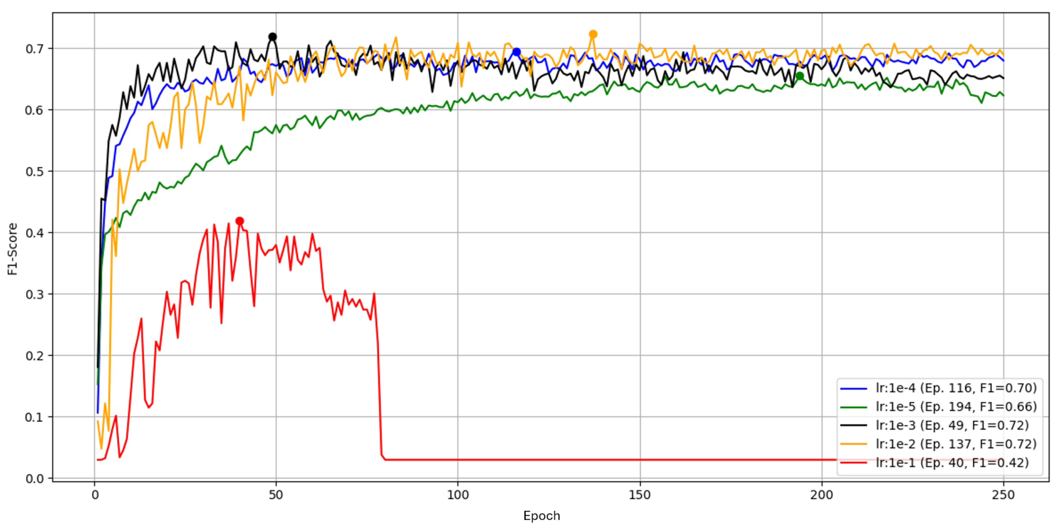
Figure 8.
Learning -rate sweep for YOLOv5 over 250 epochs on Part A, position 1, measured by F1.
The largest rate, , peaks at F1 then diverges after epoch 83 (F1 drops to 0/NaN). The default reaches a transient peak of at epoch 137 but is unstable and otherwise plateaus near . A rate of yields the best balance with a stable peak of by epoch 49; behaves similarly but tops out at . The smallest rate, , is stable but underfits and remains . We therefore proceed with for this configuration.
Loss Weights (box and class)
We tuned the loss-component gains for box and class. Five evenly spaced values were used per axis, producing runs (Table 6) and the corresponding F1 curves in Figure 9.
Performance varies noticeably with the weighting. The global best within this grid is box=0.155 with class=2.250 (F1 at epoch 181), closely followed by box=0.065 with class=4.300 (F1 ). With low box loss (), higher class loss helps; with high box loss (), F1 declines. Very low class loss () underperforms (F1 , stagnating by epoch 59). The top configurations are summarized in Table 7.
Summary for Part A
Relative to the baseline F1 of at , increasing the input to raised F1 to . Learning-rate tuning showed that extreme values are harmful or unstable, while provided the best stability-speed trade-off for this setup. Finally, adjusting box/class loss gains increased F1 further to .
To assess overfitting, Figure 10 plots training and validation losses; the vertical line marks the epoch of peak F1. Training losses decrease steadily, but the validation box loss rises after epoch 45, indicating the onset of overfitting despite a continued slight decrease of validation class loss. This supports monitoring beyond a single F1 peak.
The final setting used in subsequent runs is listed in Table 8.
2.6.1. Results on Part A
Using the settings from Table 8, we trained one model per position and one joint model on all positions. Figure 11 shows the best F1 per position; scores range from (POS6) to (POS2), mean with a span of .
Figure 12 relates F1 to the number of annotations per position. No linear relationship is evident; positions with more annotations do not necessarily achieve higher F1, and the position with the most annotations shows the lowest F1.
Figure 13 relates F1 to average annotation area. Again, no clear relationship appears; F1 varies despite increasing average area for several positions. Thus, neither count nor area alone explains the F1 variability.
The joint model trained on all positions reaches a maximum F1 of , which is below the mean of the nine position-specific models (Figure 14). While the joint model sees more variability during training, it may generalize better to unseen defect patterns. A further fine-tuning in the joint setting could improve results, but was not feasible here due to training time constraints.
In the practical evaluation, we compare both approaches qualitatively on example images.
2.7. Hyperparameter Optimization on Part B
The optimization approach used for Part A was transferred to Part B (H530H). The dataset used was position 6 with 150 images and ∼1700 annotations. We first varied the input resolution; results are shown in Figure 15.
As with Part A, the native resolution yields the highest F1, ranging from 0.55 up to 0.73. At the default the curves fluctuate less than in Part A; differences appear mainly as a vertical shift relative to higher resolutions.
Learning Rate
With the input fixed at , the learning rate was swept over the same interval as in Part A.
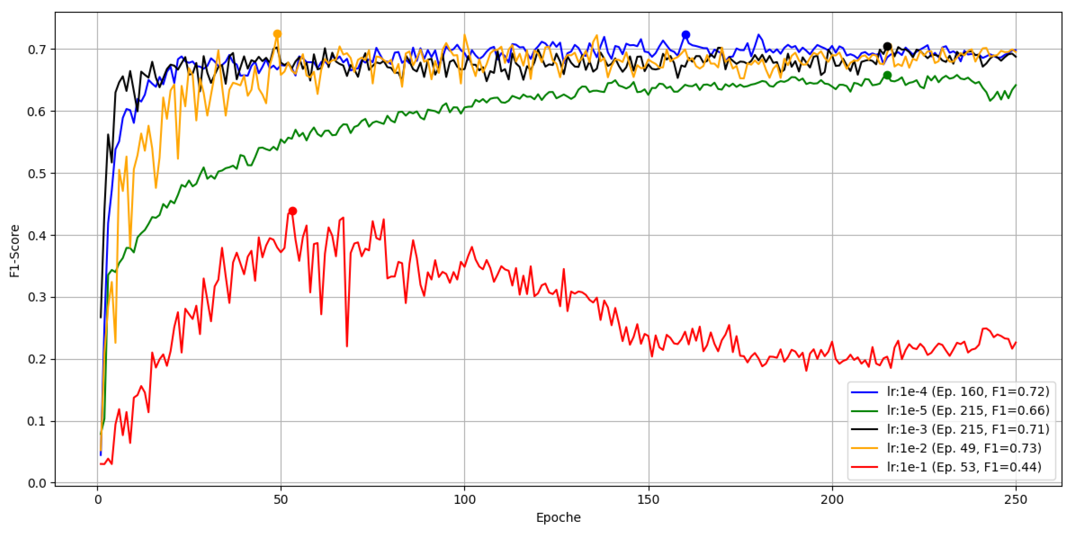
Figure 16.
Learning-rate sweep for YOLOv5 over 250 epochs on Part B, position 6, measured by F1.
The largest rate gives the worst convergence. It does not crash but declines after a peak near epoch 53. The smallest rate behaves like in Part A and appears stuck in a local minimum. The remaining three rates are similar; the best peak F1 of 0.73 occurs with around epoch 49.
Loss Weights (box and class)
Box and class loss gains were tuned over 25 combinations; Figure 17 shows the best F1 per pair.
Overall peak F1 is 0.697 at , , reaching its maximum by epoch 45. With no further improvement is observed (best , F1 , epoch 116). With , the second-best result is F1 at by epoch 24, while higher class weights reduce performance (e.g., 0.672 at 4.300, epoch 130). With , the best is F1 at by epoch 93; very high class weight underperforms (0.679 at 4.300, epoch 182). With , the best is F1 at by epoch 37; larger class weights again degrade results.
None of the loss-weight combinations surpassed the F1 from the learning-rate optimization; the top loss-weight result is about 3% lower than the LR peak (cf. Figure 16). A check of defaults showed the library’s box loss gain set near , while the documented tuning range here was –. Despite being only suggested ranges, the default is orders of magnitude higher than the explored grid.
2.7.1. Results on H530H (Part B)
As in Part A, we trained one model per position and one joint model on all positions, each with the best tested hyperparameters for Part B. The best F1 per position is shown in Figure 18.
F1 ranges from 0.72 to 0.85 with a mean of 0.79, a span of . Figure 19 and Figure 20 show F1 versus annotation count and average annotation area. No clear relationship is evident.
A joint model trained on the full H530H dataset is shown in Figure 21. Its peak F1 is again about 0.02 below the mean of the position-specific models. As with Part A, practical tests compare both approaches on example images to assess generalization to previously unseen defects.
2.8. Practical Live Test
The purpose was to validate shop-floor readiness on legacy X-ray equipment and benchmark the system against certified inspectors with emphasis on critical defects. The test spanned two calendar weeks. During this period, all sampled images deemed critical were stored and included in the evaluation; in addition, 10 randomly selected images per part were added for a complete comparison. A blind, paired evaluation was conducted: for each part, the system and the inspectors reviewed exactly the same image set. Both model types were tested in parallel: a position-specific model (trained per position) and a part-level model (trained on all positions of the part). For critical defects, the check was limited to whether the model detected the same findings that the materials inspector reported. Images were frozen before the test; no retraining was performed. The operating point was fixed from validation, and disagreements were adjudicated to form ground truth.
2.8.1. Metrics
Per-class Precision, Recall, and F1 were reported. False-positive rate and review time per image were recorded where applicable. Throughput and latency were not measured in this test.
2.8.2. Connection Between GUI and X-Ray System
As outlined in Section Industrial Context and Equipment, the cell uses VistaPlusV for acquisition and viewing, which exposes no API. To enable automated ingestion by the evaluation software, the vendor’s user-defined processing scripts are extended to save each acquired image using:
PartName_Position_Timestamp
Images are written to a predefined base path on an internal network share; with a daily subfolder created automatically. The evaluation software watches this share, parses PartName and Position, and triggers the corresponding model.
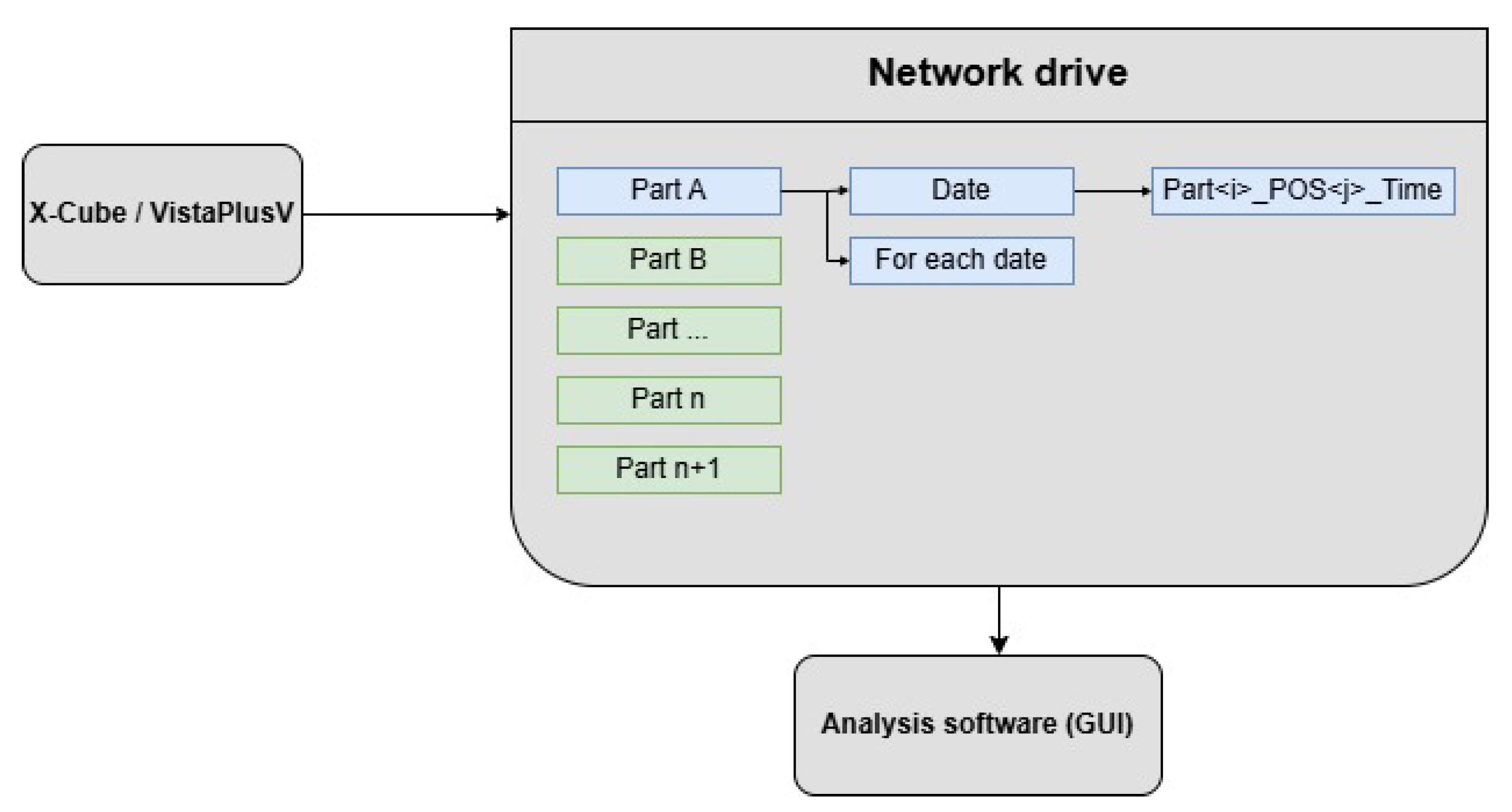
Figure 22.
Connection between GUI and X-ray System
This file-based bridge is robust and non-invasive; no changes to VistaPlusV or the X-ray hardware are required.
2.8.3. Review of Critical Defects
Part A (H183H). Seven images were flagged as critical (n.i.O.) by inspectors. Both models were tested: the position-specific model detected 7/7 critical findings; the part-level model detected 6/7.
Qualitative finding (Part A).
Both models correctly locate the defect; the position-specific model produces higher confidence than the part-level model.
Part B (H530H). Eleven images were flagged as critical. Both models were tested and detected all relevant critical findings; the position-specific model produced tighter boxes.
Qualitative finding (Part B).
The part-level model undersegments and assigns lower confidence than the position-specific model.
2.8.4. Review of All Defects (10 Random Images per Part)
Ground truth considerations.
There is no universal ground truth for non-critical defects. All comparisons are relative between the system and certified inspectors on the same images. Disagreements were adjudicated. To avoid over-counting, split detections that referred to one physical defect were merged (“cleaning”), so each defect is counted once.
Part A (H183H).
Before cleaning, inspectors lead on F1 with strong recall; both models show high precision but lower recall (Table 9). After cleaning (Table 10), the picture tightens: inspectors drop slightly, while both models gain recall and F1 because merged splits reduce missed counts relative to correct counts. Net: inspectors remain best on Part A, but the position-specific model closes much of the gap; the part-level model improves yet remains behind.
Interpretation (Part A). Cleaning reduces inflated counts from fine splits. Inspector F1 drops slightly (0.916 → 0.904). The position-specific model gains recall (0.716 → 0.814) and F1 (0.830 → 0.892) at constant precision; the part-level model improves to 0.849 F1.
Part B (H530H).
Before cleaning, precision is near-perfect for all cohorts; recall drives differences (Table 11). After cleaning (Table 12), both models gain evidently because merged splits convert multiple near-duplicates into single correct detections, increasing recall without harming precision. Net: on Part B both models surpass inspectors on F1, with a slight edge for the part-level model.
Interpretation (Part B). Cleaning lowers inspector F1 (0.843 → 0.806) as close marks are merged; both models improve recall and F1 (position-specific 0.821 → 0.891; part-level 0.837 → 0.904).
Overall outcome.
Cleaning aligns evaluation with physical defects and rewards detectors that produce consolidated boxes rather than many small splits. After cleaning, the position-specific model remains competitive and nearly closes the gap to inspectors on Part A, while on Part B both models exceed inspector performance with high precision and improved recall.
3. Results
3.1. Runtime and Model Family
3.2. Baseline: YOLO Variant Selection
On an identical reference setup (Part A, POS2; 250 epochs), all modern YOLO variants reached similar peak F1; YOLOv5 achieved the highest peak (0.59 at epoch 142) and the fastest time-to-best (10.20 min). v9 was close in F1 but slower; v10 was markedly slower without higher F1 (Figure 4, Table 4). We proceeded with YOLOv5.
3.3. Hyperparameter Gains
Input resolution dominated performance. Raising from to increased Part A’s F1 from 0.59 to 0.73 (Figure 7) at higher training cost (Table 5). With resolution fixed at 2016, tuning yielded a best of F1=0.755 for Part A at , , (Figure 8 and Figure 9; Table 7). For Part B, native resolution again performed best, peaking at F1=0.73 with (Figure 15, Figure 16, Figure 17).
3.4. Position-Specific vs. Part-Level Models
With the tuned settings, position-specific models achieved F1=0.74–0.87 (mean 0.78) on Part A and 0.72–0.85 (mean 0.79) on Part B (Figure 11, Figure 18). The part-level model per part peaked about ∼0.02 below the average of the position-specific models (Figure 14 and Figure 21). In the live test, both model types ran stably in real time.
3.5. Critical-Defect Performance (Live)
Part A. Inspectors flagged 7 critical images. The position-specific model detected 7/7; the part-level model 6/7. The example in Figure 23 shows both detections with higher confidence for the position-specific model. Part B. Inspectors flagged 11 critical images. Both models detected all relevant critical findings; the position-specific model produced tighter boxes (Figure 24).
3.6. Comparison with Inspectors on All Defects (Live)
Paired evaluation used identical images per cohort. Disagreements were adjudicated; split detections were merged to count physical defects. Part A. Inspectors remained best after cleaning (F1 0.904); the position-specific model was close (0.892); the part-level model trailed (0.849) (Table 9, Table 10). Part B. Both models surpassed inspectors after cleaning (position-specific 0.891, part-level 0.904, inspector 0.806) (Table 11, Table 12).
3.7. Overall Takeaways
A CPU-feasible one-stage detector with native-resolution inputs and modest tuning achieves competitive porosity detection. Position-specific models yield tighter localization and higher confidence; part-level models trade some localization for cross-position generalization and performed best on Part B under live conditions. Integration via a file-based bridge was robust and maintained qualitative real-time behavior on the shop floor.
4. Discussion
This study demonstrates that a one-stage detector can satisfy stringent shop-floor constraints for porosity detection in aluminum die-cast radiographs while achieving competitive accuracy relative to certified inspectors. The three central outcomes—real-time CPU feasibility, strong resolution sensitivity, and the granularity trade-off between position-specific and part-level models—directly address RQ1–RQ3. Under CPU-only deployment, YOLOv5 met the s latency target, whereas the two-stage baseline did not, aligning with prior findings that one-stage architectures provide superior throughput on non-GPU hardware [4,5]. Maintaining the native spatial resolution () delivered the largest accuracy gains, confirming that small, low-contrast porosity signatures require high-resolution inputs [3]. Model granularity shaped performance: position-specific models yielded sharper localization at the trained pose, while the part-level model generalized better across poses and slightly exceeded inspectors on one part.
Comparable patterns are reported in other industrial and medical DL applications. In industrial surface-inspection systems, Lu and Lee demonstrate real-time defect detection using a lightweight YOLO-based network, though their deployment relies on GPU acceleration, highlighting that many industrial workflows meet throughput requirements via dedicated hardware rather than CPU-only execution [11]. In medical imaging, by contrast, object-detection models such as Faster R-CNN, RetinaNet, or YOLOv5 are commonly used in offline diagnostic pipelines, where inference times of several seconds are acceptable and accuracy is prioritized over strict latency constraints, as reviewed by Elhanashi et al. [12]. These cross-domain observations emphasize that the s requirement addressed in this study is domain-specific and significantly stricter than typical inspection or diagnostic settings.
4.1. Interpretation Relative to Hypotheses and Prior Work
The results support all hypotheses without requiring restatement of the findings. H1 is validated by the clear latency separation between one-stage and two-stage models, consistent with analyses attributing throughput advantages to shared backbone computation and simplified detection heads. H2 is supported by the strong dependency of detection quality on input resolution, extending prior work by demonstrating that this effect persists under strict CPU-only deployment constraints. H3 is reflected in the observed trade-off between specialization and generalization: view-specific training sharpens decision boundaries but reduces robustness, whereas pooled training broadens coverage at the cost of localization precision. These interpretations position the present findings as aligned with, and extending, established theoretical and empirical work in industrial vision.
4.2. Implications for Industrial Practice.
For safety-critical inspection, the live-test analysis indicates that the risk of missing critical defects can be controlled with a CPU-feasible pipeline when the operating point is fixed from validation and when high-resolution inputs are used. Counting rules materially affect perceived performance. Merging split detections into single physical defects (“cleaning”) produced a modest decrease in inspector F1 and a concomitant increase in model recall and F1, suggesting that detectors tend to fragment extended porous regions. Consequently, operational KPIs should be reported on physical defects rather than raw mark counts to avoid bias against automated systems that intentionally over-segment for safety.
4.3. Limitations.
The study analyzes two parts in one production cell and one defect class (porosity) on 2D radiographs; external validity to other parts, exposure recipes, or CT data remains untested. The live-test samples for critical defects were small, so uncertainty is non-negligible. For non-critical findings, ground truth required adjudication and thus retains residual subjectivity. Finally, throughput and latency were not instrumented during the live test; only qualitative real-time behavior was observed.
4.4. Future Directions.
Three extensions are immediate. First, broader prospective studies with instrumented logging should quantify end-to-end latency, cold-start effects, and operator interaction time. Second, small-budget automated tuning constrained to deterministic hyperparameters may reduce calibration effort across parts and positions. Third, post-processing that learns to consolidate neighboring boxes could reduce split detections without degrading recall. Additional opportunities include calibrated uncertainty for triage, periodic active learning from adjudicated disagreements, and evaluation on multi-class defect scenarios and CT volumes.
5. Conclusions
A deployable, CPU-only pipeline for automated porosity detection in production radiographs is feasible on legacy X-ray equipment using a non-invasive, file-based interface. Among evaluated detectors, the one-stage family met strict latency targets; with native-resolution inputs and modest deterministic tuning, YOLOv5 achieved competitive accuracy. In live operation, all critical defects were detected on one part and nearly all on the other, meeting the primary acceptance focus. When evaluation counts are aligned to physical defects, automated models match or exceed inspector performance in representative settings.
For practice, position-specific models are preferable where tight localization at a fixed pose is paramount; part-level models are advantageous when cross-position generalization and workflow simplicity are prioritized. Adoption should fix the operating point, retain high-resolution inputs when computation permits, and report KPIs after consolidating split detections. Under these conditions, AI-assisted inspection can improve consistency and reduce the risk of missed critical defects in aluminum die casting while operating within existing IT and hardware constraints.
References
- Ren, S.; He, K.; Girshick, R.; Sun, J. Faster R-CNN: Towards Real-Time Object Detection with Region Proposal Networks. arXiv preprint arXiv:1506.01497, 2015. Available online: https://arxiv.org/abs/1506.01497 (accessed on 21 November 2025).
- Jocher, G.; Chaurasia, A.; Qiu, J. YOLOv5: An Improved Version of YOLO for Object Detection (Technical Report). Ultralytics, 2020. Available online: https://github.com/ultralytics/yolov5 (accessed on 21 November 2025).
- Zhang, X.; Liu, J.; Wang, H.; Zhao, L. A Novel Deep Learning Network for Small-Defect Detection in Aluminum Castings Using Wasserstein-Based Loss Functions. Scientific Reports 2025, 15, 90185. Available online: https://www.nature.com/articles/s41598-025-90185-y (accessed on 21 November 2025).
- Parlak, O.; Yurdakul, B.; Gül, R.; Karas, I.R. Automated defect detection in aluminum castings using deep learning on X-ray images. Engineering Applications of Artificial Intelligence 2022, 114, 105075.
- Yılmaz, B.; Arslan, A.; Demir, M. Deep learning-based detection of aluminum casting defects and their types using YOLOv5. Journal of Manufacturing Processes 2023, 94, 528–538.
- Fortune Business Insights. X-ray Inspection System Market Size, Share & Industry Analysis, 2024–2032. Available online: https://www.fortunebusinessinsights.com/x-ray-inspection-system-market-105227 (accessed on 20 September 2025).
- Reuters. Key energy output data track Germany’s economic revival. Reuters 2025. Available online: https://www.reuters.com/markets/commodities/key-energy-output-data-track-germany-charts-economic-revival-maguire-2025-02-25 (accessed on 20 September 2025).
- Reuters. Germany plans to cut energy costs by 42 billion euros, draft budget shows. Reuters 2025. Available online: https://www.reuters.com/sustainability/germany-plans-cut-energy-costs-by-42-billion-euros-draft-budget-shows-2025-07-28 (accessed on 20 September 2025).
- Tzutalin. LabelImg (software); GitHub, 2015. Available online: https://github.com/tzutalin/labelImg (accessed on 26 September 2025).
- BDEW. BDEW-Strompreisanalyse Oktober 2025: Haushalte und Industrie; BDEW Bundesverband der Energie- und Wasserwirtschaft e.V.: Berlin, Germany, 2025. Available online: https://www.bdew.de/service/daten-und-grafiken/bdew-strompreisanalyse/ (accessed on 20 September 2025).
- Lu, J.; Lee, S.-H. Real-Time Defect Detection Model in Industrial Environment Based on Lightweight Deep Learning Network. Electronics 2023, 12, 4388. Available online: /mnt/data/electronics-12-04388.pdf (accessed on 21 November 2025).
- Elhanashi, A.; Saponara, S.; Zheng, Q.; Almutairi, N.; Singh, Y.; Kuanar, S.; Ali, F.; Unal, O.; Faghani, S. AI-Powered Object Detection in Radiology: Current Models, Challenges, and Future Direction. J. Imaging 2025, 11, 141. Available online: /mnt/data/jimaging-11-00141.pdf (accessed on 21 November 2025).
Figure 1.
Annotations per inspection position for Part A (POS1–POS9). Bars show total porosity annotations per position; dashed line indicates the median across positions.
Figure 1.
Annotations per inspection position for Part A (POS1–POS9). Bars show total porosity annotations per position; dashed line indicates the median across positions.
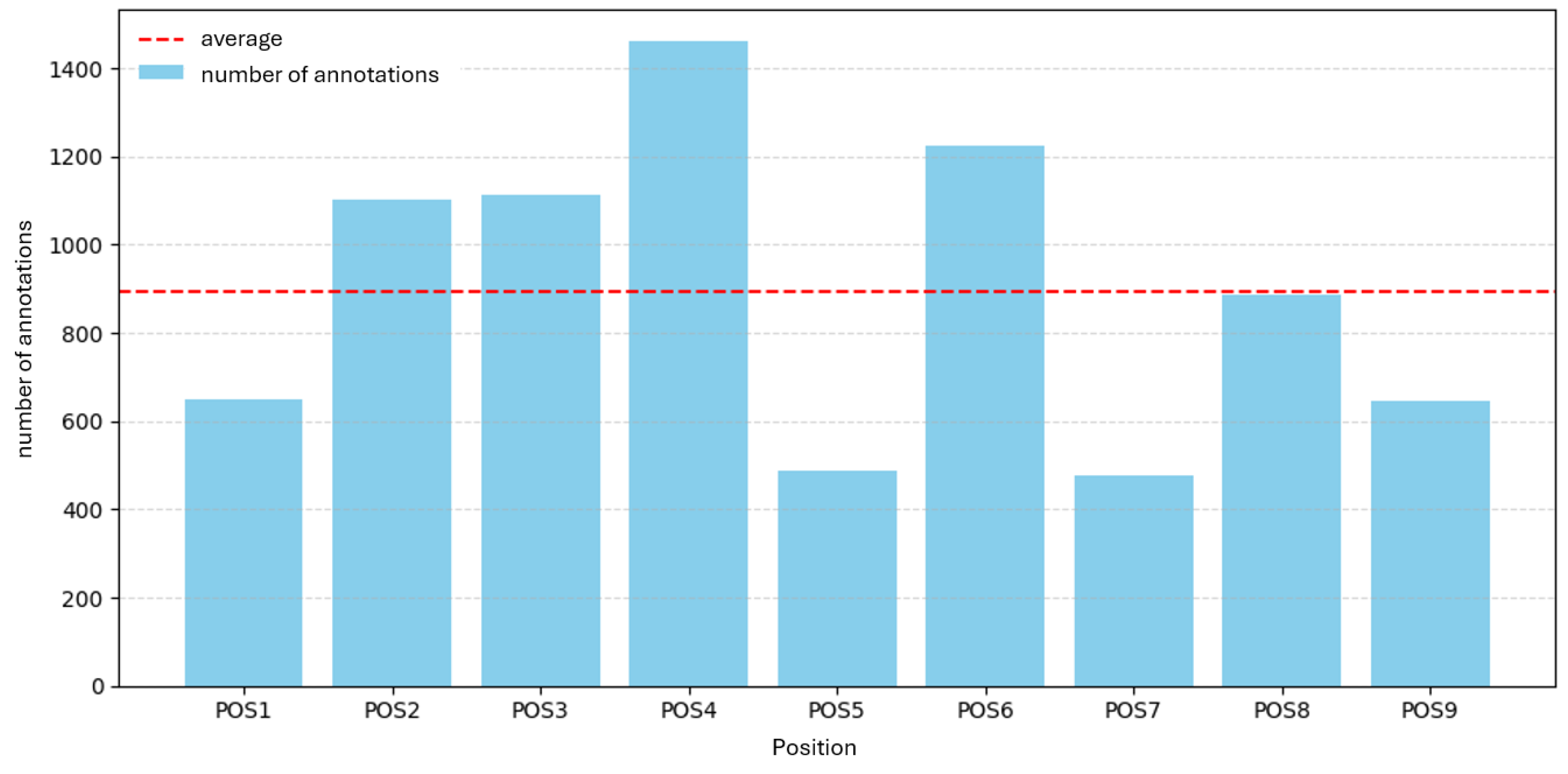
Figure 2.
Annotations per inspection position for Part B (POS1–POS18). Bars show total porosity annotations per position; dashed line indicates the median across positions.
Figure 2.
Annotations per inspection position for Part B (POS1–POS18). Bars show total porosity annotations per position; dashed line indicates the median across positions.
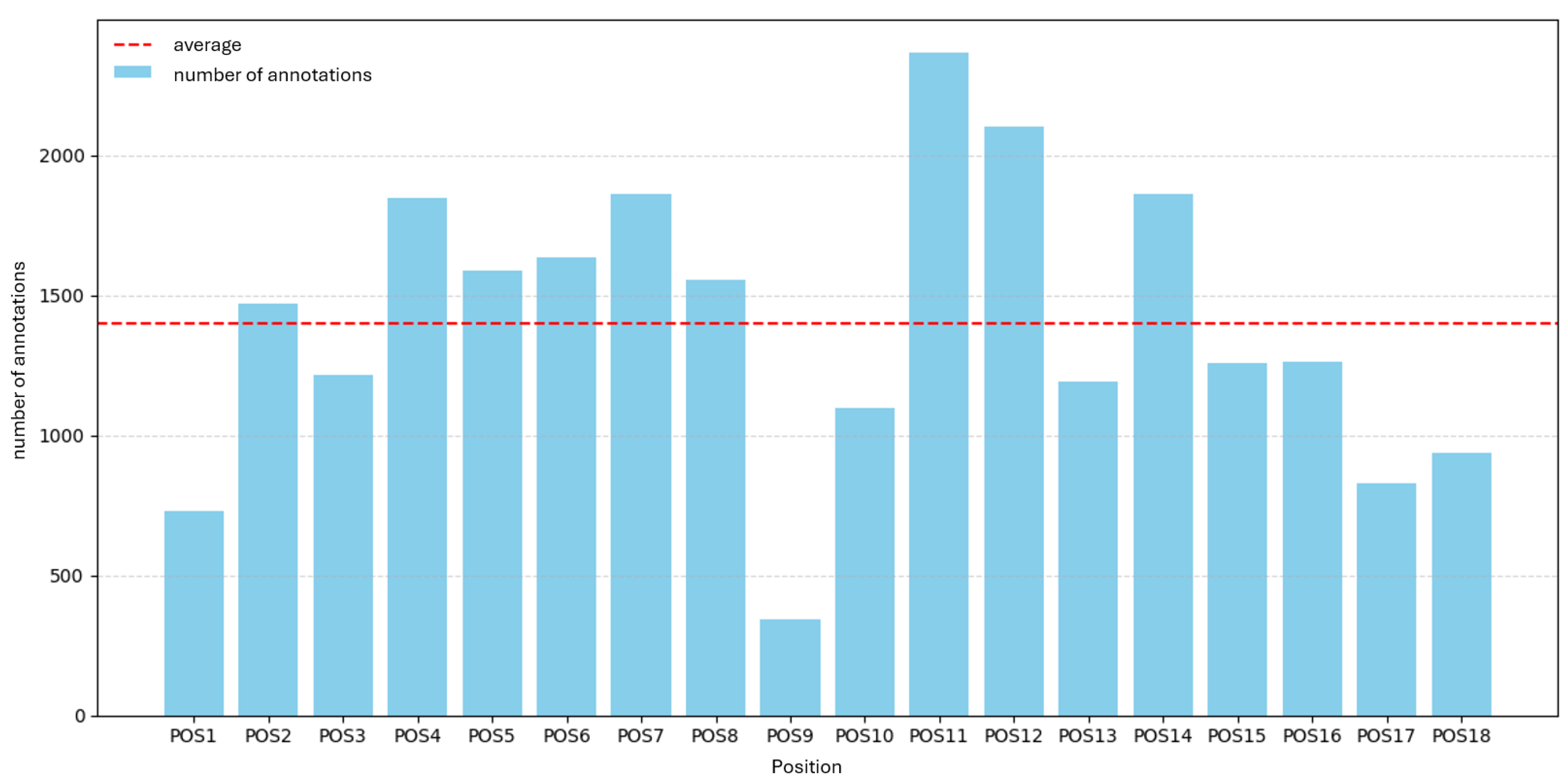
Figure 5.
Procedure for model training and hyperparameter optimization.
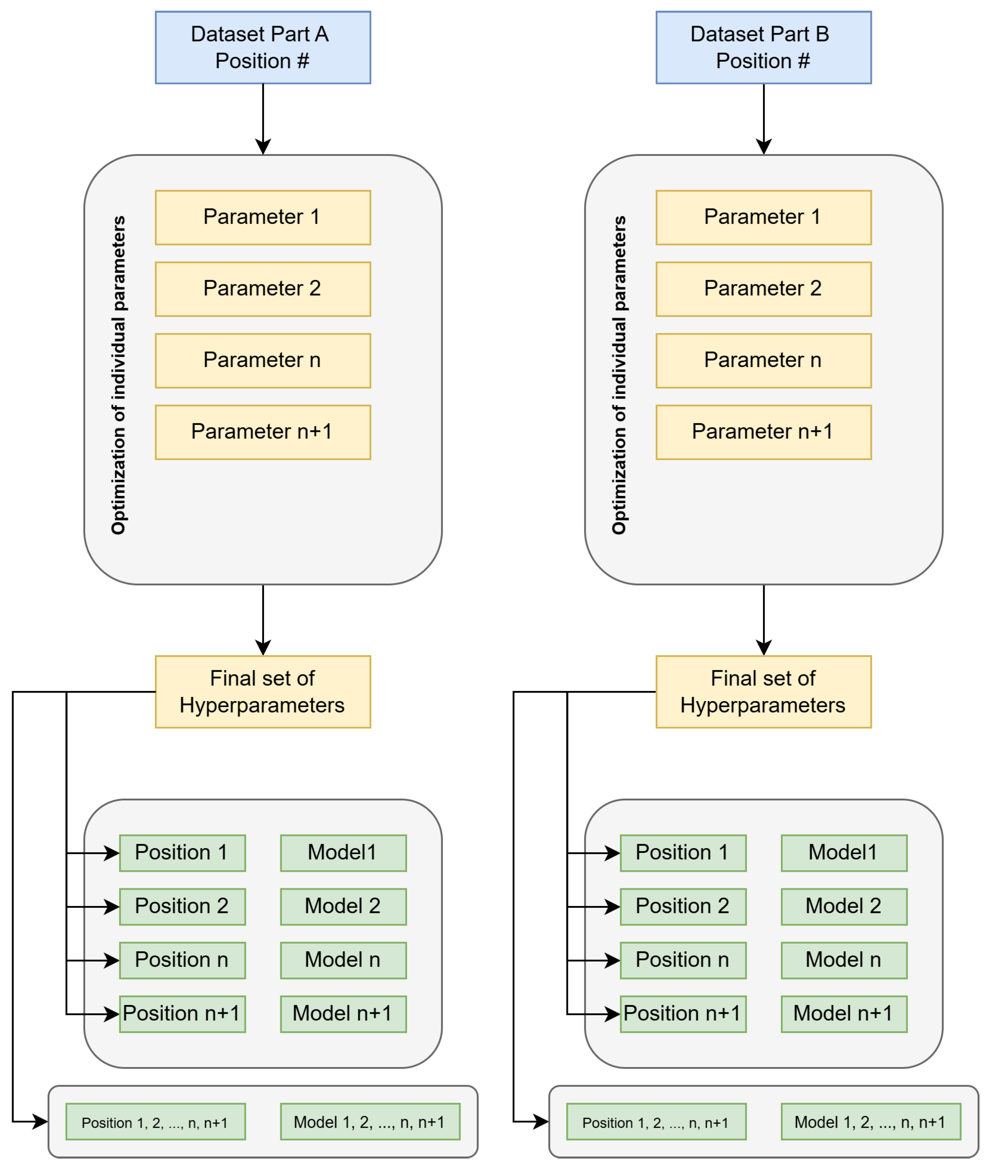
Figure 6.
Identical defects in the microstructure: a) original resolution (), b) downscaled ().
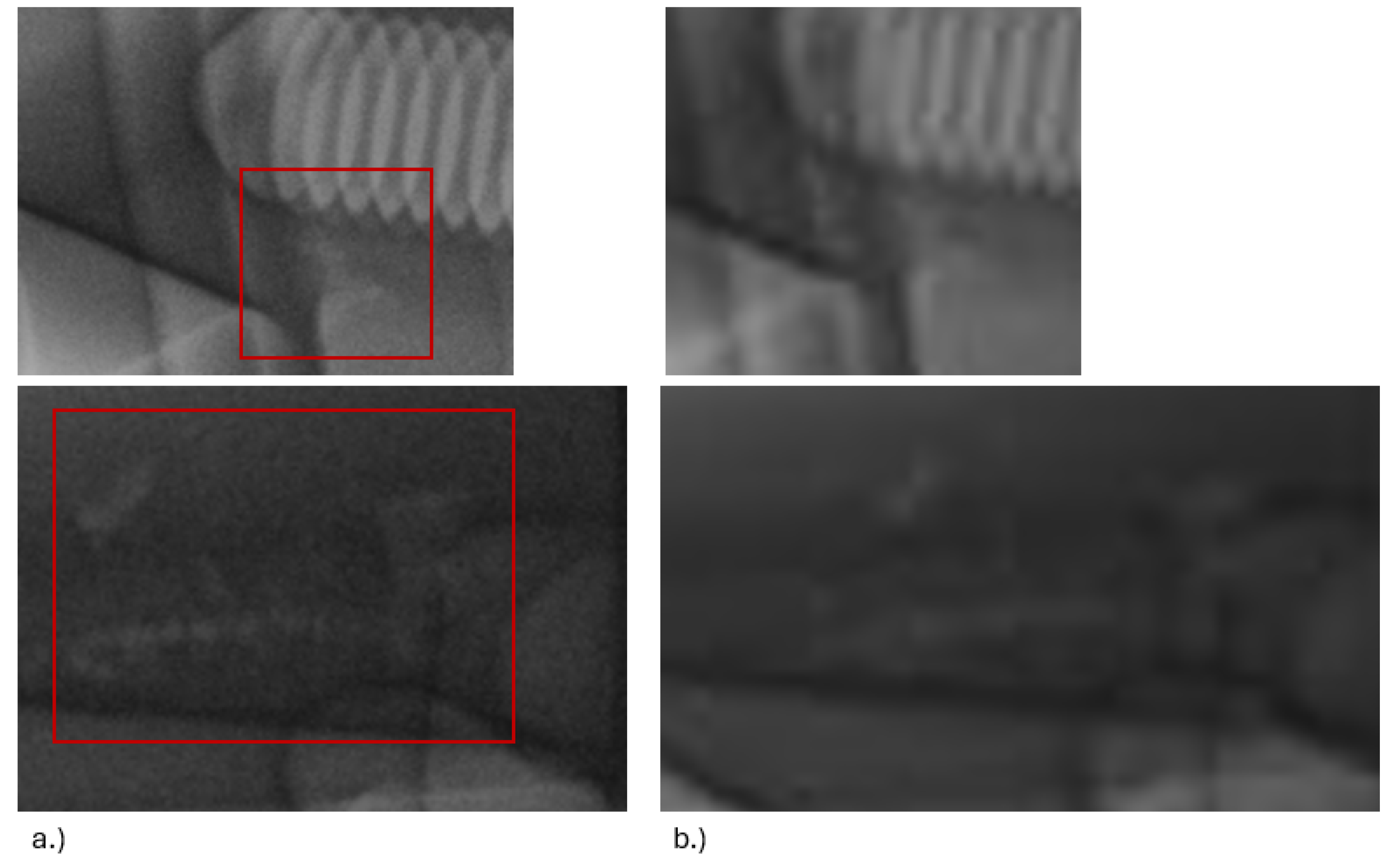
Figure 7.
YOLOv5 across input resolutions over 250 epochs on Part A, position 1, measured by F1.
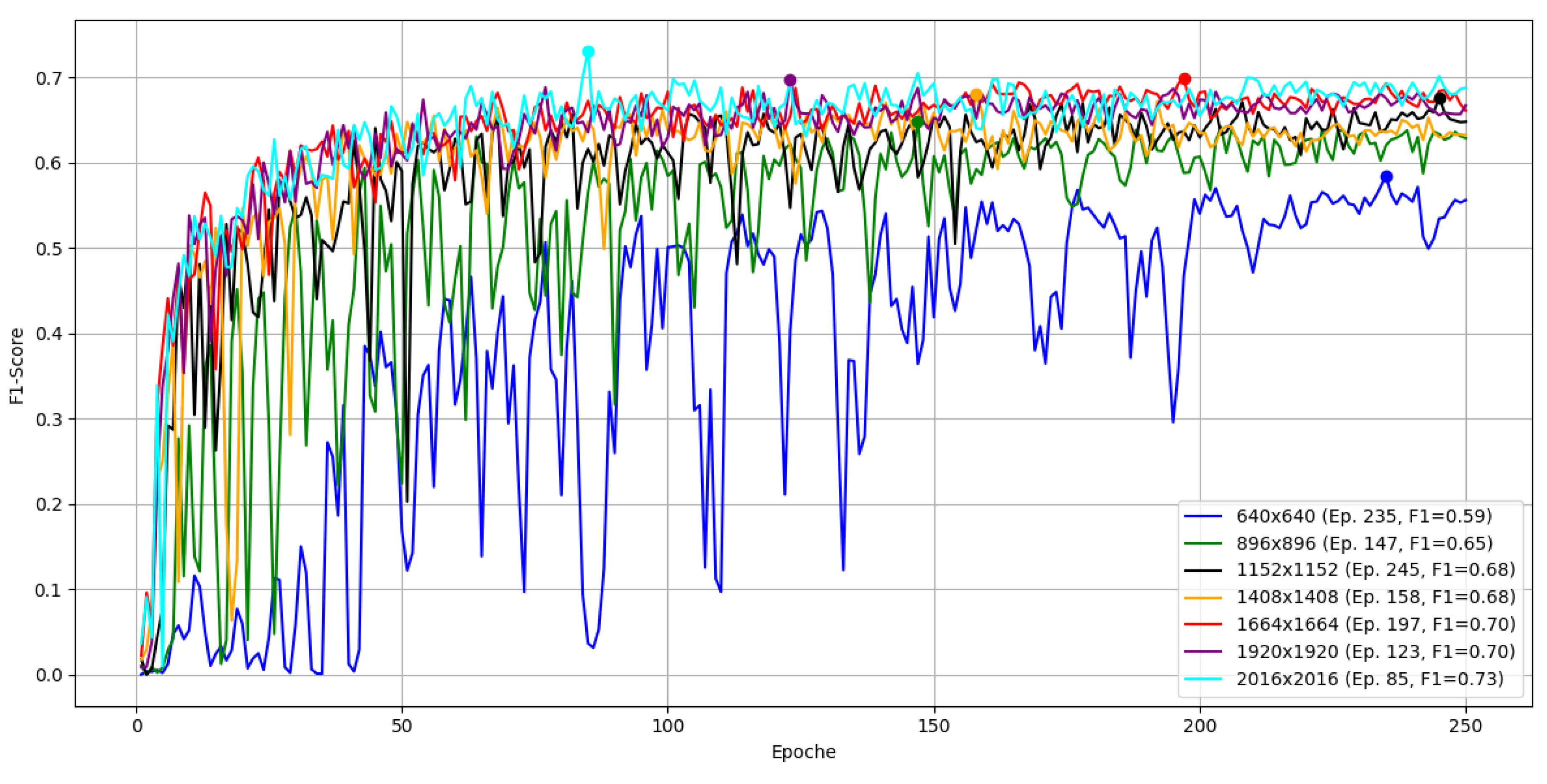
Figure 9.
F1 over 250 epochs for combinations of box and class loss gains.
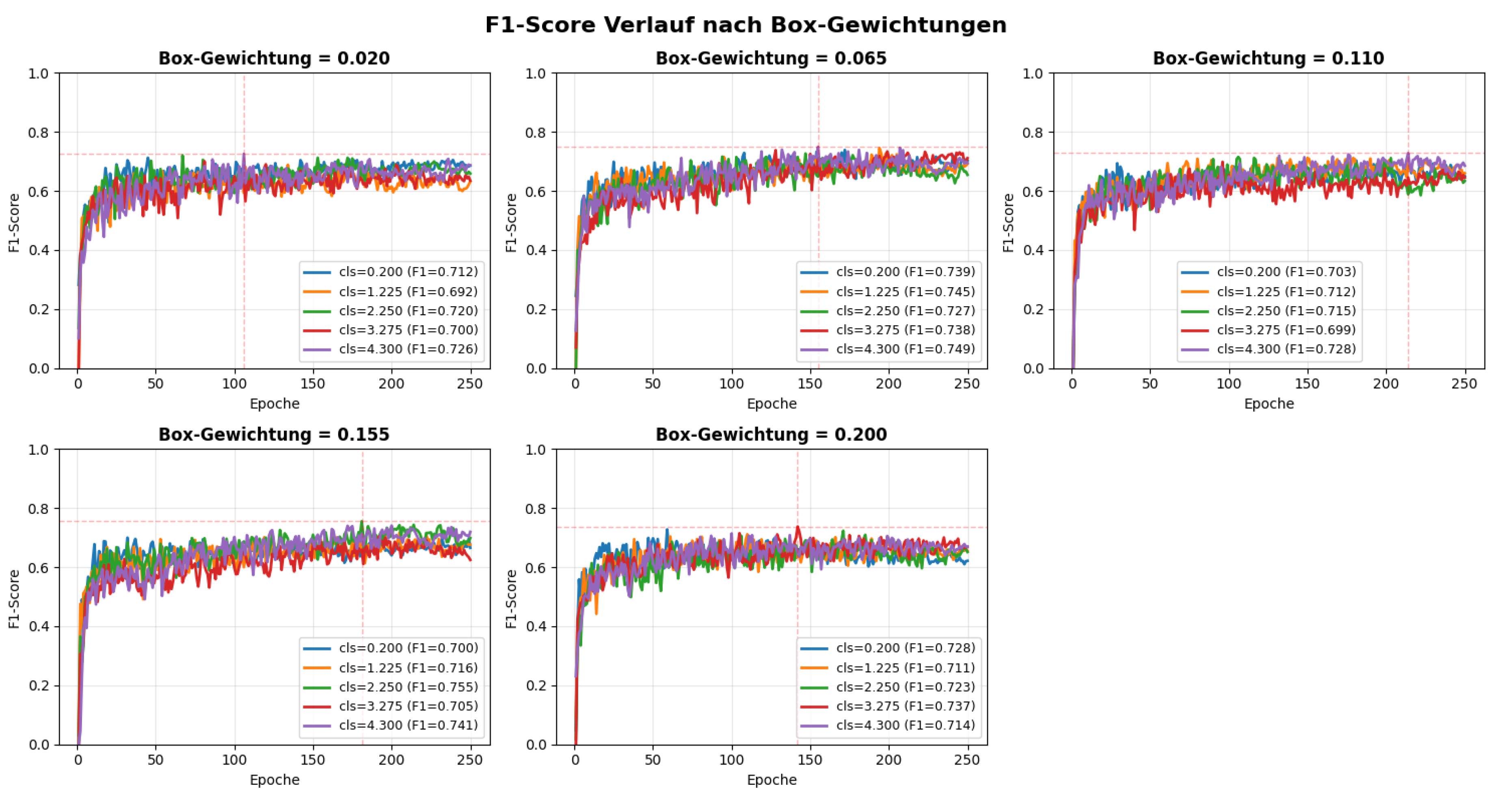
Figure 10.
Training and validation losses over time. Vertical line: epoch of peak F1.
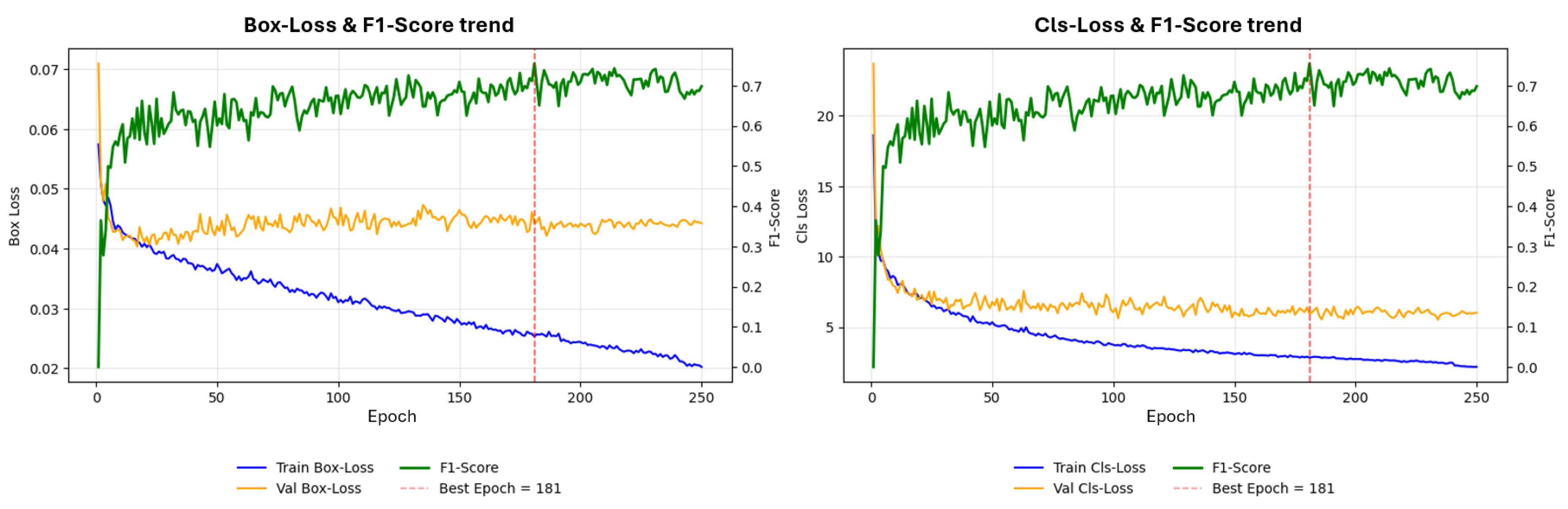
Figure 11.
Best F1 per position for H183H (Part A).
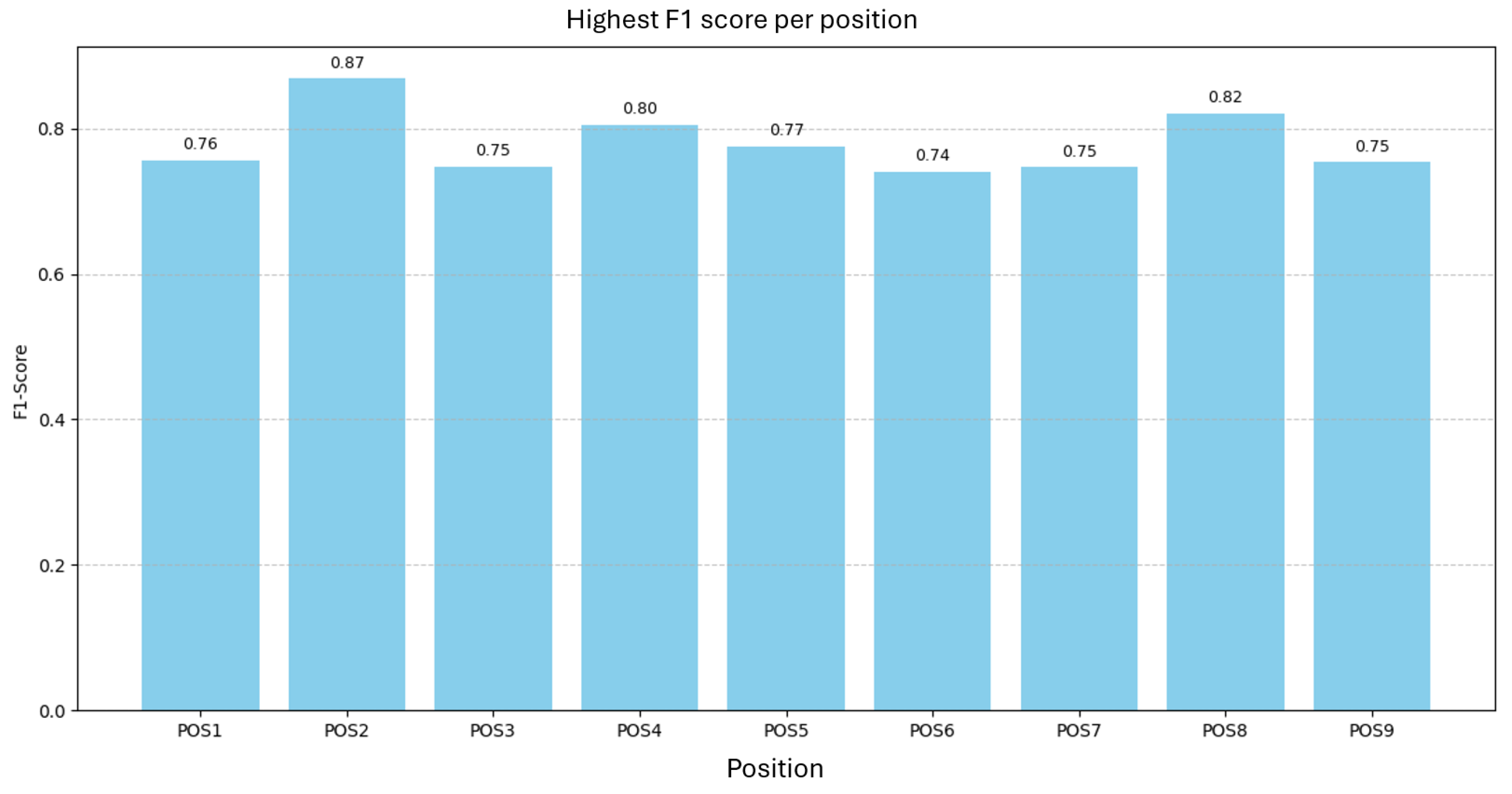
Figure 12.
F1 versus number of annotations per position for H183H.
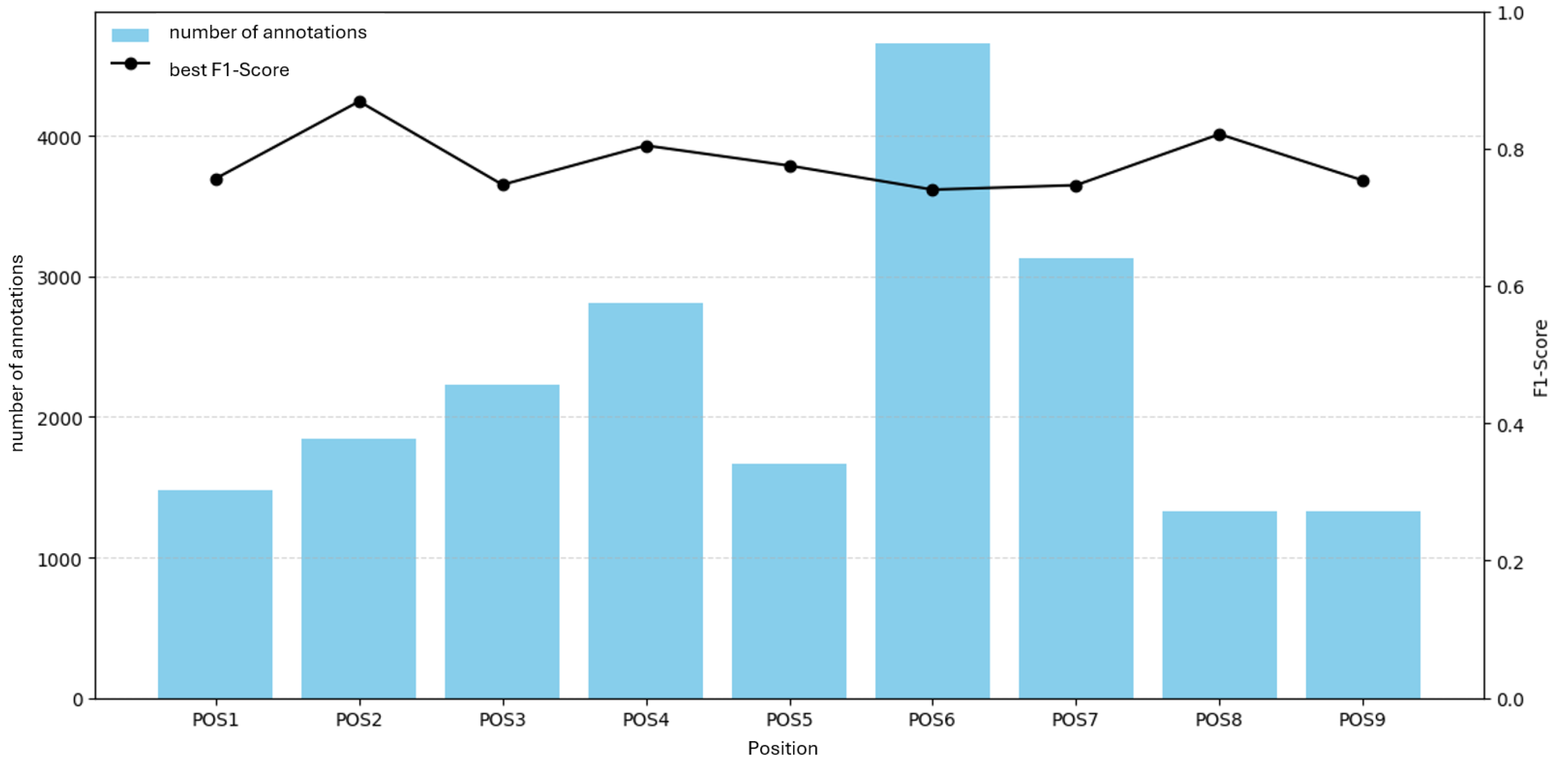
Figure 13.
F1 versus average annotation area per position for H183H.
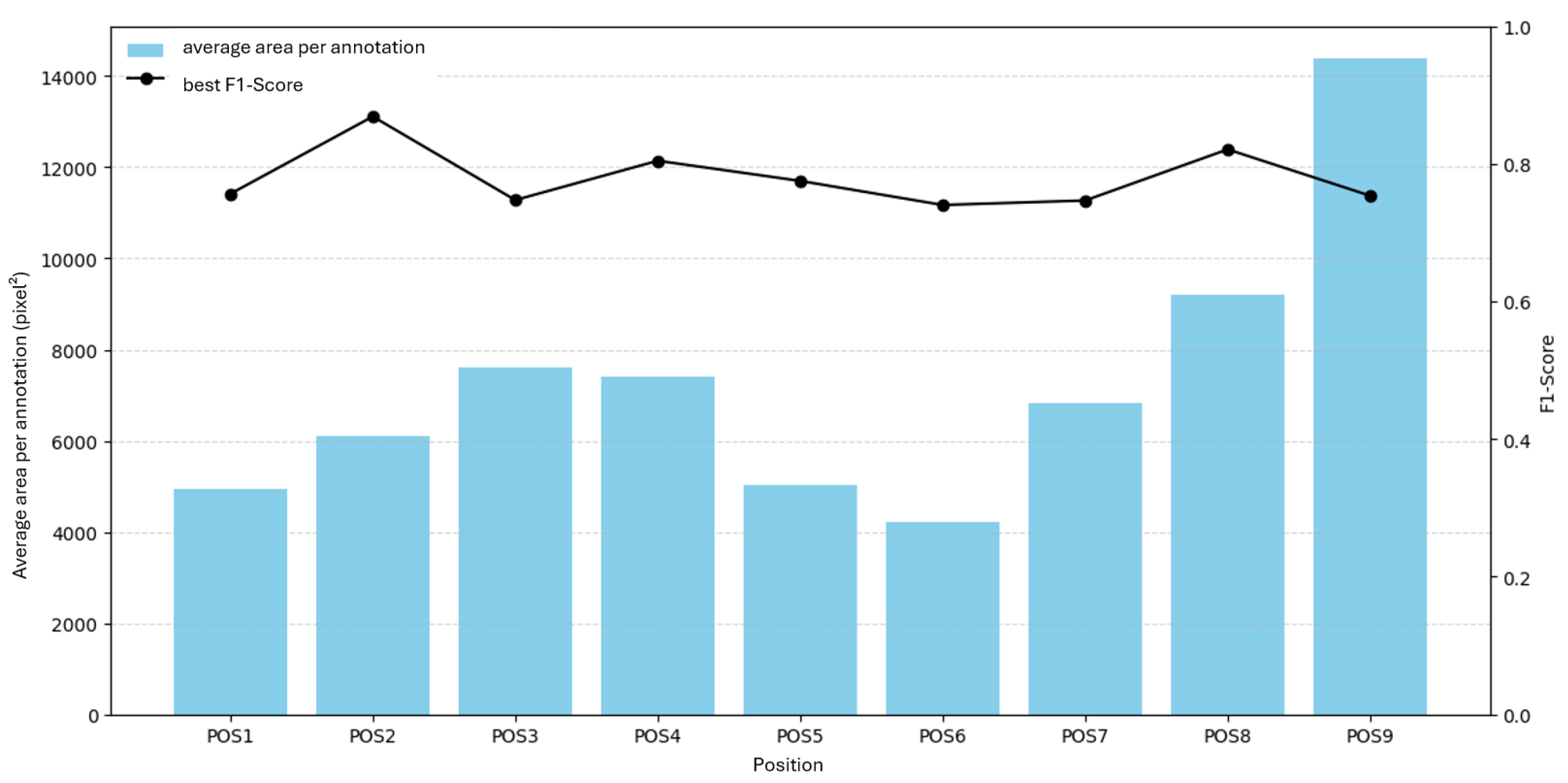
Figure 14.
F1 over epochs using the full H183H dataset (joint model).
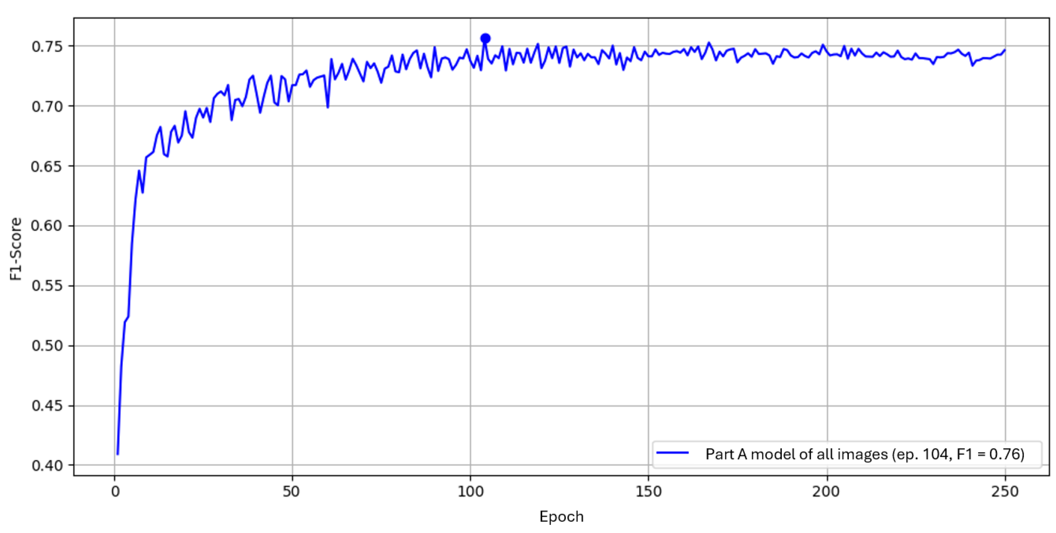
Figure 15.
YOLOv5 across input resolutions over 250 epochs on Part B, position 6, measured by F1.
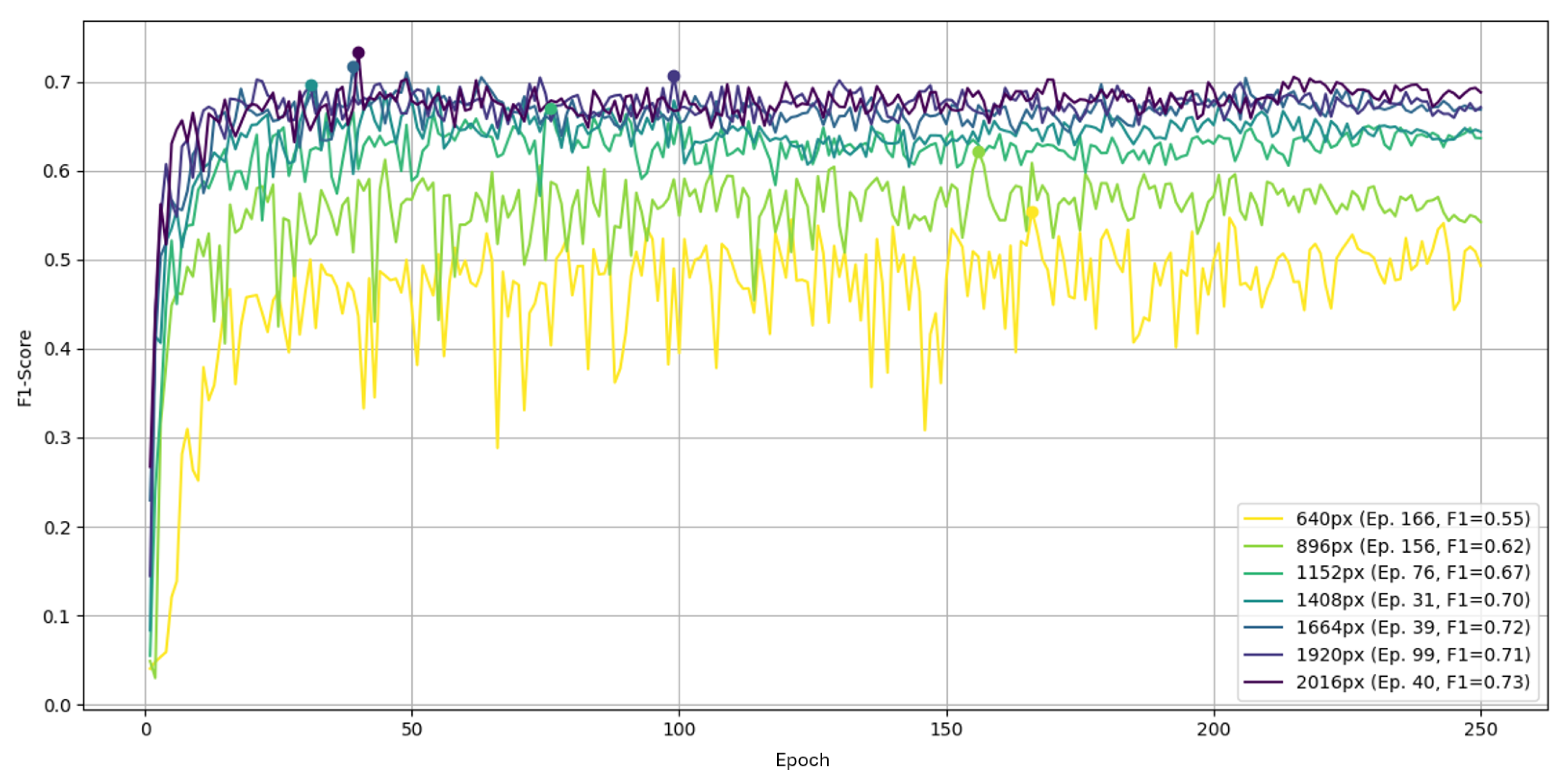
Figure 17.
Heatmap of peak F1 across box and class loss gains on Part B over 250 epochs.
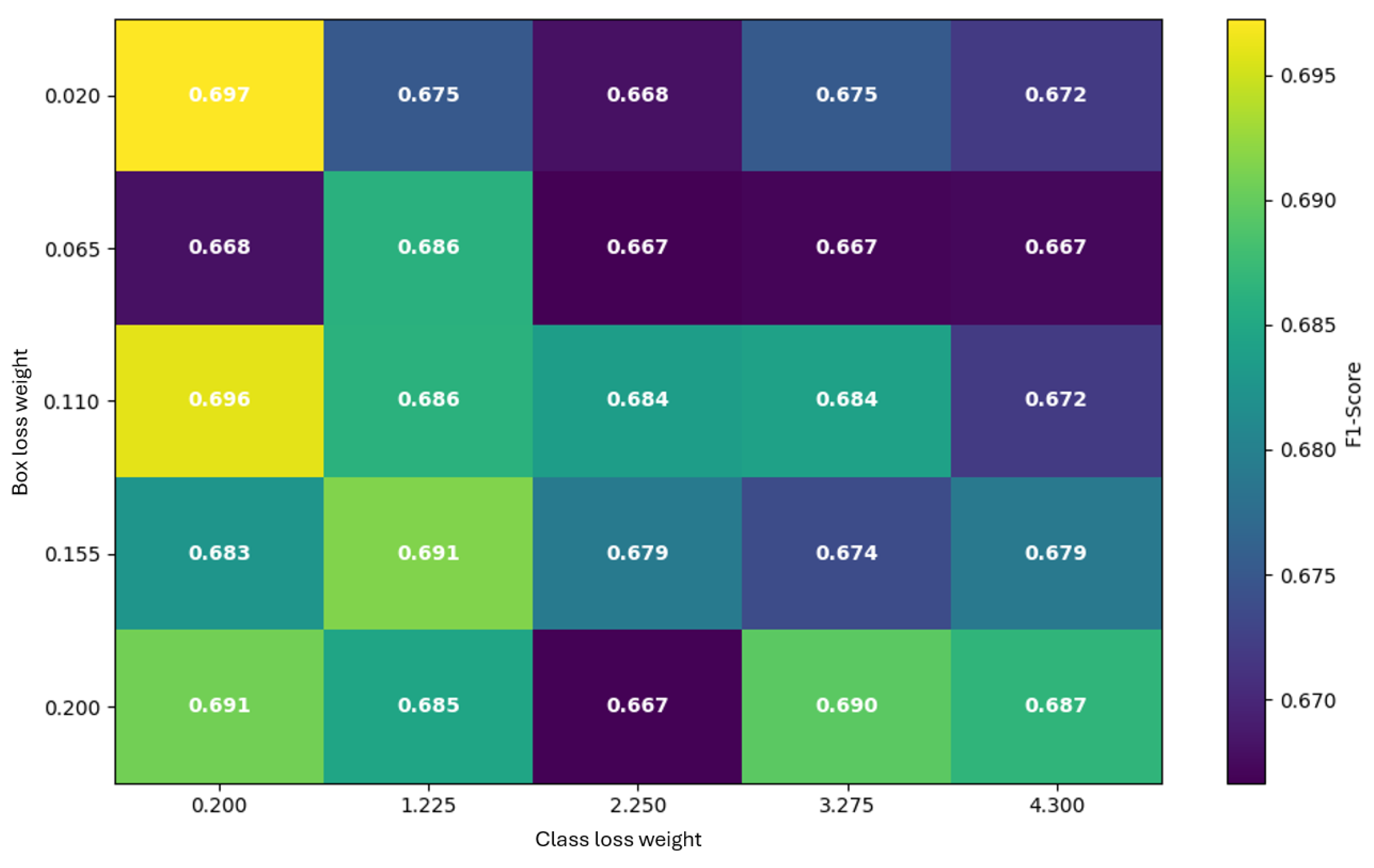
Figure 18.
Best F1 per position for H530H (Part B).
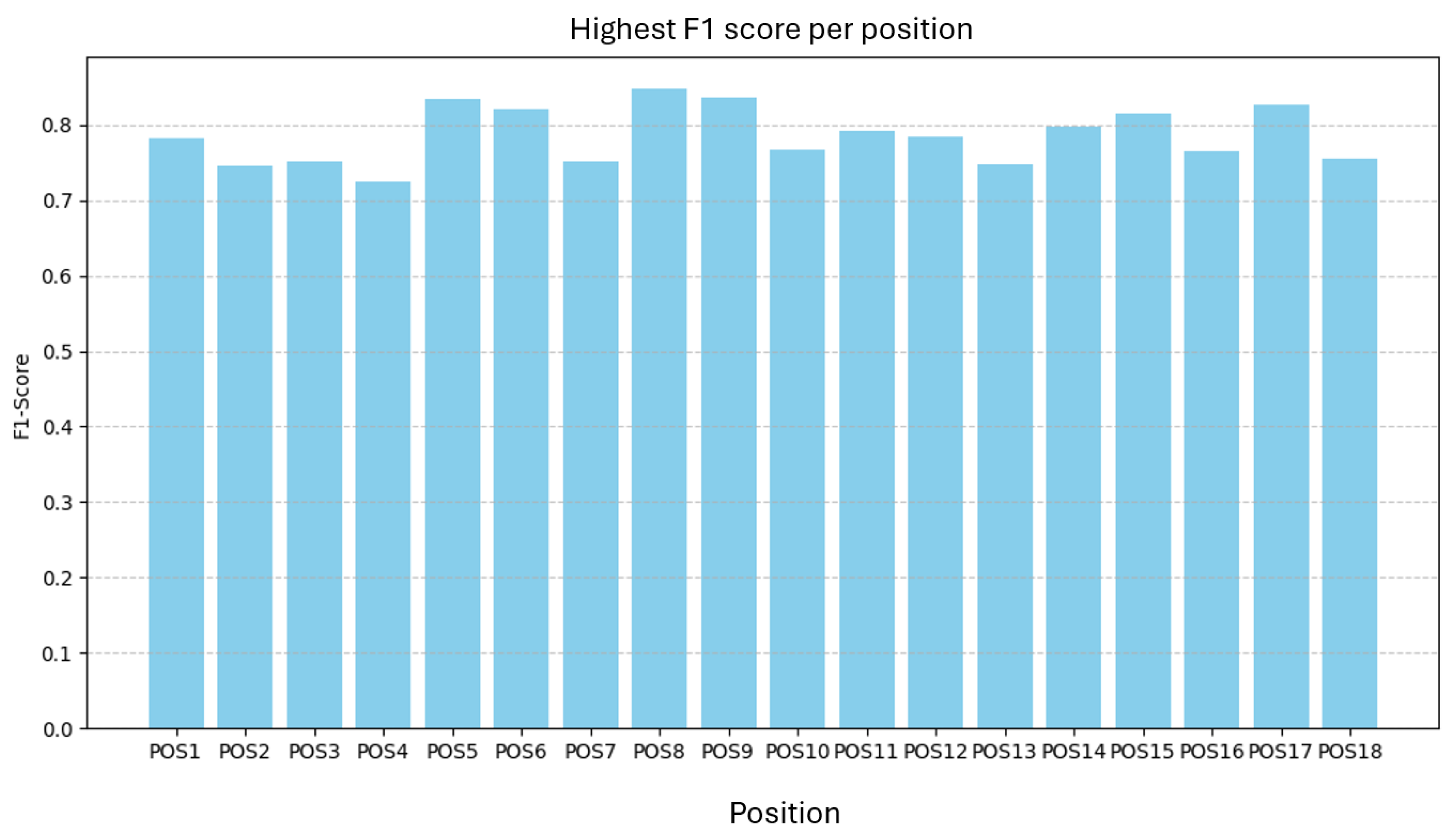
Figure 19.
F1 versus number of annotations per position for H530H.
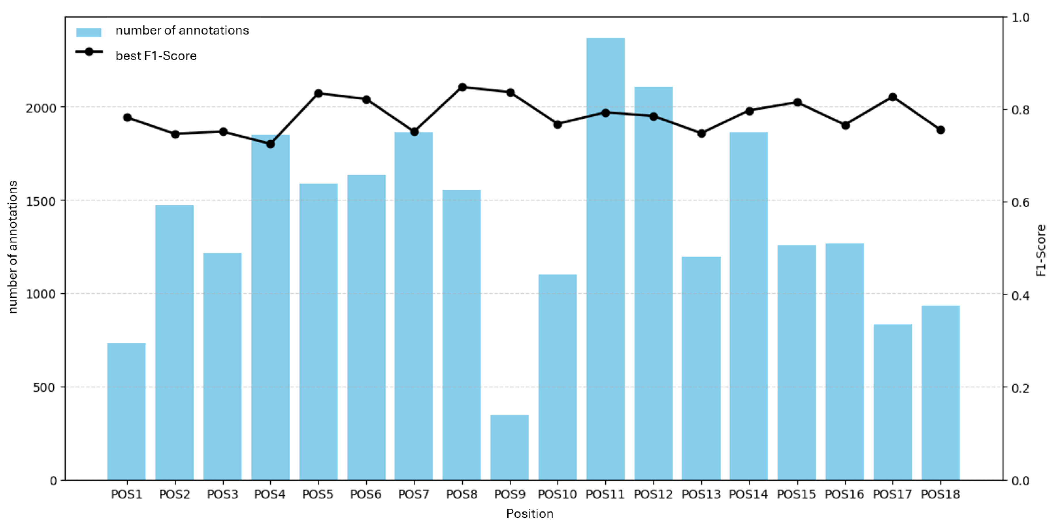
Figure 20.
F1 versus average annotation area per position for H530H.
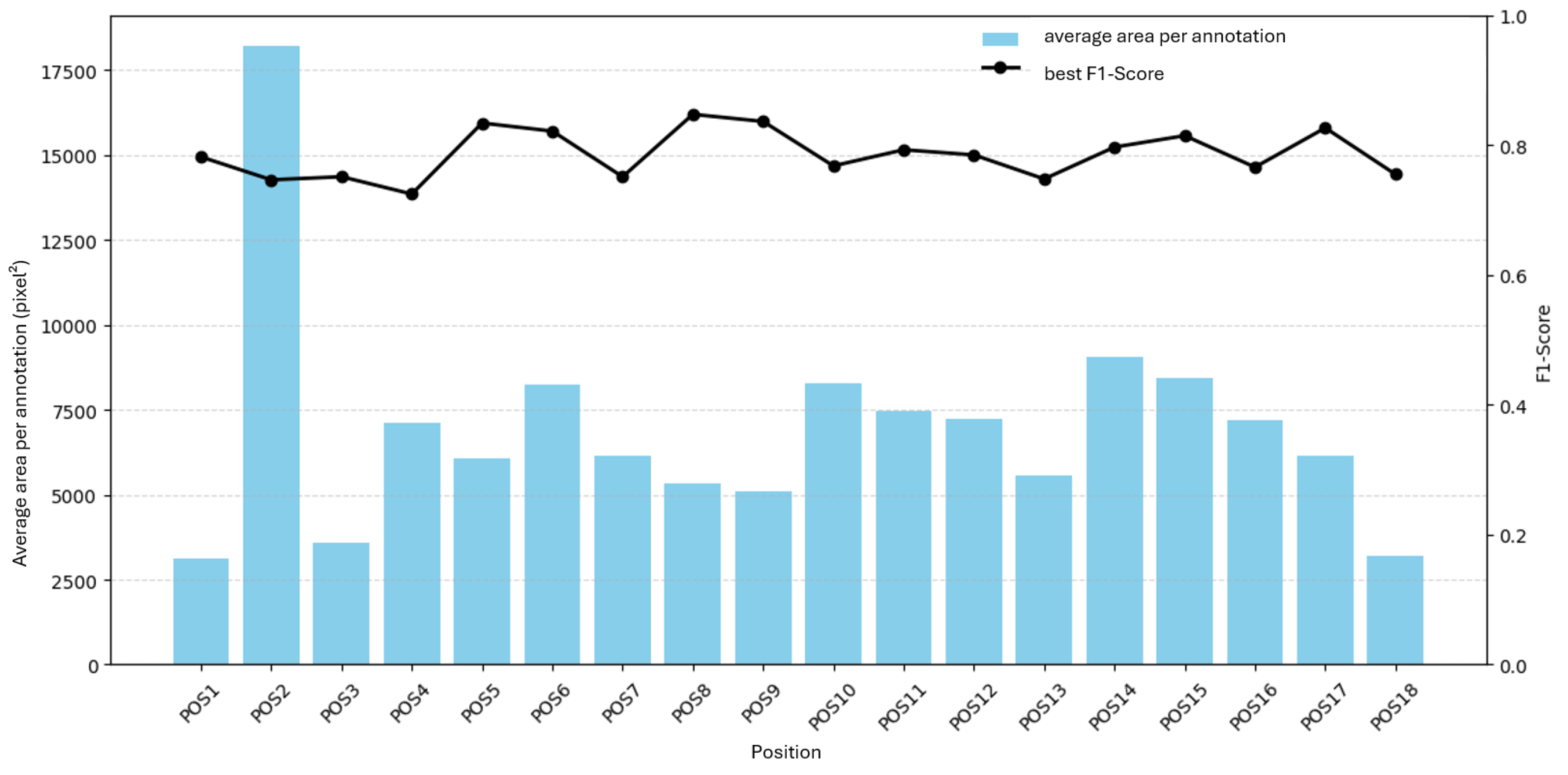
Figure 21.
F1 over epochs using the full H530H dataset (joint model).
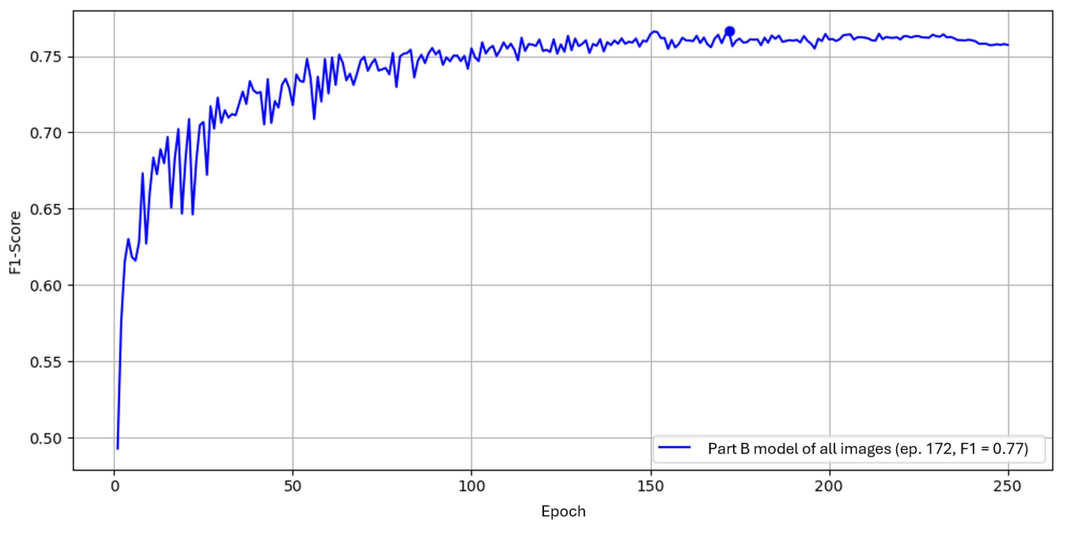
Figure 23.
Critical example for Part A: M1 (position-specific) vs. M2 (part-level). Both detect the defect, with M1 assigning higher confidence; confidence values indicate detector certainty but are not used in the evaluation.
Figure 23.
Critical example for Part A: M1 (position-specific) vs. M2 (part-level). Both detect the defect, with M1 assigning higher confidence; confidence values indicate detector certainty but are not used in the evaluation.
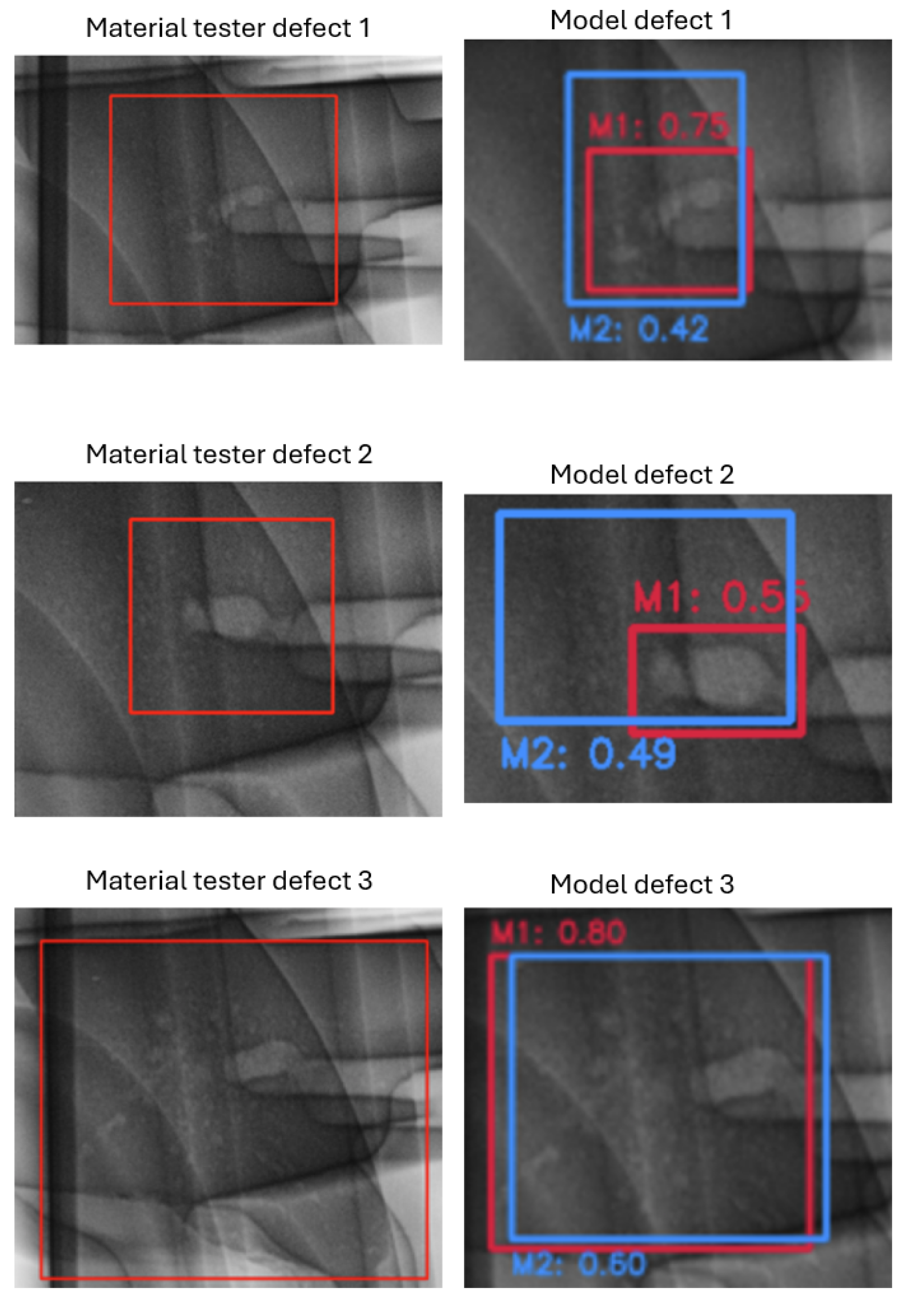
Figure 24.
Critical example for Part B: M1 (position-specific) vs. M2 (part-level). M2 localizes the defect only partially and at lower confidence; M1 provides fuller coverage with higher confidence.
Figure 24.
Critical example for Part B: M1 (position-specific) vs. M2 (part-level). M2 localizes the defect only partially and at lower confidence; M1 provides fuller coverage with higher confidence.
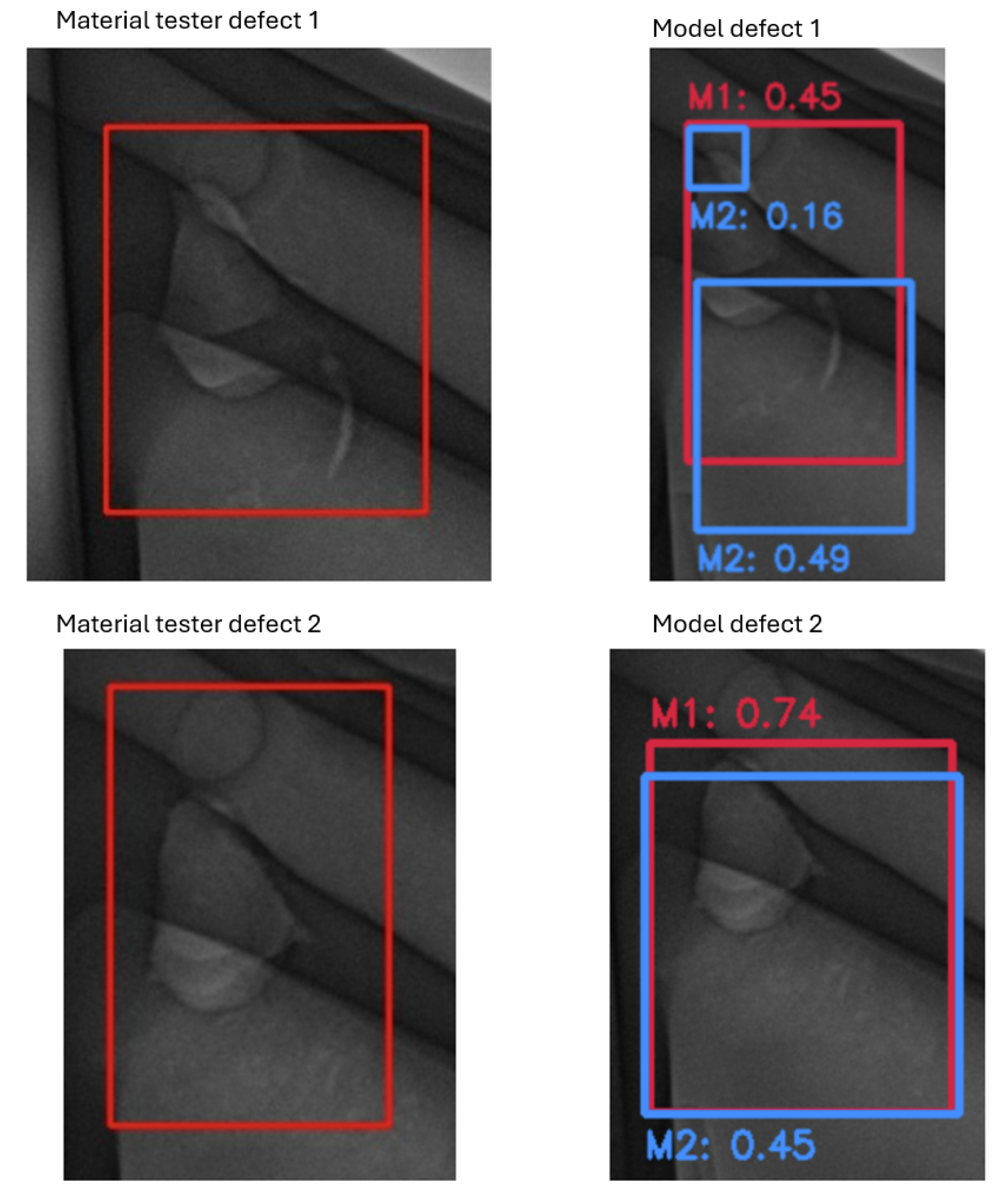

Table 1.
Aggregate dataset summary for anonymized components.
| Component | #Positions | Images (total) | Annotations (total) | Images/Position (median) |
|---|---|---|---|---|
| Part A | 9 | 2,700 | 12,960 | 300 |
| Part B | 18 | 2,700 | 27,443 | 150 |
Files follow a minimal scheme: PartA_POS<k> / PartB_POS<k>.
Table 2.
Industrial PC (inference target) hardware and OS.
| Component | Specification | Notes |
|---|---|---|
| CPU | Intel Core i5-13500 | 14 cores / 20 threads (6P + 8E), CPU-only |
| RAM | 16 GB | |
| GPU | — | No discrete GPU |
| Storage | SSD (industrial grade) | |
| OS | Windows 11 Enterprise | Endpoint security active |
| Runtime | Single-file EXE (PyInstaller) | No Python env on host |
Used for all CPU latency measurements and shop-floor deployment.
Table 3.
CPU runtime preselection on the industrial PC (batch size 1; timed runs; first run discarded from the mean).
Table 3.
CPU runtime preselection on the industrial PC (batch size 1; timed runs; first run discarded from the mean).
| Framework | Source image (px) | Model input (px) | Mean [s] | Min / Max [s] |
|---|---|---|---|---|
| YOLOv5 (pretrained) | 2016×2016 | 640×640 | 1.33 | 1.261 / 2.39 |
| Faster R-CNN (pretrained) | 2016×2016 | 640×640 | 5.59 | 3.718 / 9.698 |
Measurements on Intel Core i5-13500, 16 GB RAM, Windows 11, CPU-only. The max for YOLOv5 is the warm-up run.
Table 4.
Training times for YOLO variants over 250 epochs.
| Model | Total time [min] | Time to best F1 [min] | Avg. time / epoch [min] |
|---|---|---|---|
| YOLOv5 | 19.08 | 10.20 | 0.08 |
| YOLOv8 | 19.39 | 10.83 | 0.08 |
| YOLOv9 | 18.60 | 12.45 | 0.07 |
| YOLOv10 | 32.16 | 20.42 | 0.13 |
| YOLOv11 | 21.47 | 18.32 | 0.09 |
Table 5.
Training time versus input resolution
| Resolution | Total (min) | Time to best F1 (min) | Avg/epoch (min) |
|---|---|---|---|
| 640x640 | 19.20 | 17.30 | 0.08 |
| 896x896 | 31.95 | 18.57 | 0.13 |
| 1152x1152 | 48.61 | 47.69 | 0.19 |
| 1408x1408 | 69.46 | 43.54 | 0.28 |
| 1664x1664 | 96.84 | 75.89 | 0.39 |
| 1920x1920 | 125.71 | 61.67 | 0.50 |
| 2016x2016 | 146.56 | 49.83 | 0.59 |
Table 6.
Grid of box and class loss weights
| Box loss / Class loss | 0.200 | 1.225 | 2.250 | 3.275 | 4.300 |
|---|---|---|---|---|---|
| 0.020 | x | x | x | x | x |
| 0.065 | x | x | x | x | x |
| 0.110 | x | x | x | x | x |
| 0.155 | x | x | x | x | x |
| 0.200 | x | x | x | x | x |
Table 7.
Effect of box and class loss weights on performance (sorted by F1)
| Box | Class | F1 | Epoch |
|---|---|---|---|
| 0.155 | 2.25 | 0.755 | 181 |
| 0.065 | 4.30 | 0.749 | 132 |
| 0.155 | 4.30 | 0.741 | 190 |
| 0.200 | 3.28 | 0.737 | 142 |
| 0.110 | 4.30 | 0.728 | 214 |
| 0.020 | 4.30 | 0.726 | 106 |
| 0.200 | 0.20 | 0.690 | 59 |
Table 8.
Best parameter set within the tested search space
| Parameter | Value |
|---|---|
| Input resolution | 2016 |
| Learning rate | |
| Class loss gain | 2.250 |
| Box loss gain | 0.155 |
Table 9.
All defects on Part A (as read, before cleaning): per-cohort counts and metrics
| Cohort | TP (Correct) | FP (False) | FN (Missed) | Precision / Recall / F1 |
|---|---|---|---|---|
| Inspector | 103 | 2 | 17 | 0.981 / 0.858 / 0.916 |
| Position-specific | 83 | 1 | 33 | 0.988 / 0.716 / 0.830 |
| Part-level | 79 | 2 | 40 | 0.975 / 0.664 / 0.790 |
Table 10.
All defects on Part A (cleaned by merging split marks): per-cohort counts and metrics
| Cohort | TP (Correct) | FP (False) | FN (Missed) | Precision / Recall / F1 |
|---|---|---|---|---|
| Inspector | 89 | 2 | 17 | 0.978 / 0.840 / 0.904 |
| Position-specific | 83 | 1 | 19 | 0.988 / 0.814 / 0.892 |
| Part-level | 79 | 2 | 26 | 0.975 / 0.752 / 0.849 |
Table 11.
All defects on Part B (as read, before cleaning): per-cohort counts and macro-averaged metrics
Table 11.
All defects on Part B (as read, before cleaning): per-cohort counts and macro-averaged metrics
| Cohort | TP (Correct) | FP (False) | FN (Missed) | Precision / Recall / F1 |
|---|---|---|---|---|
| Inspector | 91 | 0 | 37 | 1.000 / 0.746 / 0.843 |
| Position-specific | 90 | 1 | 38 | 0.996 / 0.712 / 0.821 |
| Part-level | 94 | 0 | 35 | 1.000 / 0.742 / 0.837 |
Table 12.
All defects on Part B (cleaned by merging split marks): per-cohort counts and macro-averaged metrics
Table 12.
All defects on Part B (cleaned by merging split marks): per-cohort counts and macro-averaged metrics
| Cohort | TP (Correct) | FP (False) | FN (Missed) | Precision / Recall / F1 |
|---|---|---|---|---|
| Inspector | 75 | 0 | 36 | 1.000 / 0.676 / 0.806 |
| Position-specific | 90 | 1 | 21 | 0.989 / 0.811 / 0.891 |
| Part-level | 94 | 0 | 20 | 1.000 / 0.825 / 0.904 |
Disclaimer/Publisher’s Note: The statements, opinions and data contained in all publications are solely those of the individual author(s) and contributor(s) and not of MDPI and/or the editor(s). MDPI and/or the editor(s) disclaim responsibility for any injury to people or property resulting from any ideas, methods, instructions or products referred to in the content. |
© 2025 by the authors. Licensee MDPI, Basel, Switzerland. This article is an open access article distributed under the terms and conditions of the Creative Commons Attribution (CC BY) license (http://creativecommons.org/licenses/by/4.0/).
Copyright: This open access article is published under a Creative Commons CC BY 4.0 license, which permit the free download, distribution, and reuse, provided that the author and preprint are cited in any reuse.


