
Submitted:
24 November 2025
Posted:
25 November 2025
You are already at the latest version
Abstract
This study examines how the clarity of frequency-domain characteristics in vibration signals influences the performance of deep learning models for bearing fault classification. Two datasets were used: the CWRU benchmark dataset, which exhibits distinct and easily separable spectral signatures across fault modes, and a custom low-speed bearing dataset in which small defects do not significantly alter the frequency spectrum. To enable a clear and interpretable comparison, we deliberately employed simplified CNN and LSTM ar-chitectures with a single core layer. This design choice allows us to directly attribute per-formance differences to the inherent learning mechanisms of each architecture rather than the complexity of the models.
Our representation analysis reveals that LSTM-F achieves the highest accuracy when the dataset contains clearly distinguishable spectral patterns, as in the CWRU case. In con-trast, CNN-S outperforms both LSTM models in the experimental datasets, where fault-induced frequency characteristics are weak or ambiguous. Representation analyses further reveal that LSTM-F relies on consistent frequency-indexed patterns, whereas CNN-S captures more complex time–frequency interactions, making it more robust under low-separability conditions.
These findings demonstrate that the optimal deep learning architecture for bearing fault classification depends on the degree of frequency separability in the data. LSTM-F is pref-erable for severe faults with distinct spectral features, while CNN-S is more effective for minor defects or systems exhibiting complex, weakly discriminative frequency behavior.
Keywords:
slewing bearing
; fault classification
; convolutional neural netwroks
; long short-term memory networks
; representation
1. Introduction
Rotating machinery is ubiquitous in mechanical systems, ranging from light-duty to heavy-duty and from high-speed to low-speed applications. Bearings are among the most critical components for ensuring smooth rotation, serving key roles in systems such as motor shafts, milling machine spindles, conveyor rollers, wind turbine blades, crane booms, radar antennas, excavator bodies, and bridge piers [1,2]. The reliability of bearings becomes particularly critical in scenarios involving low-speed rotations and substantial mechanical stresses. Bearings predominantly experience malfunctions caused by faults in the inner race (IF), outer race (OF), or rolling elements (RF) [3,4,5,6]. These failures can severely degrade manufacturing quality or even cause catastrophic accidents, making accurate fault mode classification essential for mechanical systems.
Traditional fault classification methods extract statistical features from vibration signals [7,8], such as acceleration, in either the time or frequency domain [9,10,11,12]. Mathematically and physically defined equations have been used to distinguish faulty bearings from normal ones [13]. However, conventional approaches often fail to detect subtle defects, making it difficult to differentiate between normal and abnormal conditions. Frequency-based techniques such as the Fourier transform are particularly limited when fault signatures are weak or ambiguous [14,15]. The problem becomes even more challenging under low-speed and slightly damaged operating conditions, where signals contain less discriminative information [16]. To address these challenges, various studies have focused on extracting weak fault features from raw vibration data. Advanced signal processing methods, such as empirical mode decomposition (EMD), can separate hidden fault-related components and identify characteristic frequencies from noisy data using the Fourier transform [17,18,19,20]. Other approaches have proposed novel fault-sensitive features [21,22], which have demonstrated higher detection sensitivity than EMD-based methods. However, these studies were typically performed under significant fault conditions, not under slight or early-stage faults. Furthermore, approaches based on [21,22] generally classify bearings only as normal or abnormal, without specifying the failure mode. Since no clear numerical threshold exists for determining fault modes, diagnosis often depends on subjective human judgment, which may lead to false positives or negatives and, consequently, severe system failures.
To overcome these limitations, data-driven methods based on deep learning have emerged, providing automatic threshold determination and fault mode identification [23,24]. Deep learning models such as convolutional neural networks (CNNs) [23] and long short-term memory networks (LSTMs) [24] have demonstrated excellent performance in bearing fault classification. Their superiority arises from their ability to uncover complex correlations between input and output data beyond human-defined engineering rules, autonomously learning discriminative features [25]. An et al. [26] proposed a bearing fault diagnosis method incorporating periodic sparse attention within an LSTM framework, achieving a 2% improvement in accuracy compared to CNN-based models. Gu et al. [27] introduced a robust fault diagnosis approach that combines discrete wavelet transforms with multi-sensor fusion through Bi-LSTM, yielding up to a 20% accuracy increase over CNN models. Li et al. [28] integrated highway gates with an attention mechanism for improved representation learning, while Li et al. [29] demonstrated that a 1D-CNN could outperform LSTM by acting as a fault-frequency band filter. Their model achieved an F1 score exceeding 98% by using a loss function designed to extract the center frequencies of fault modes selectively. Zhang et al. [30] further showed that a CNN-based model, when combined with short-time Fourier transform (STFT) features, achieved 99.96% accuracy, outperforming a bidirectional LSTM model (96.15%). Yang et al. [31] proposed converting 1D vibration signals (n²×1) into 2D images (n×n) to be processed by CNNs, achieving a 7% accuracy improvement over LSTM when using a random forest classifier.
As summarized in [26,27,28,29,30,31], deep learning methods have substantially improved the accuracy of bearing fault diagnosis. However, results remain inconsistent regarding whether CNN-based or LSTM-based models are more effective. More importantly, most comparative studies utilize complex, deep models with multiple layers and sophisticated components. While these models achieve high accuracy, their “black-box” nature makes it difficult to discern whether performance differences stem from the core architectural principles of CNNs and LSTMs or simply from the model’s depth and complexity. This presents a fundamental challenge for both researchers and engineers when selecting an appropriate model under limited computational resources and for understanding the underlying failure mechanisms. Therefore, it is necessary to investigate when and why each architecture performs better at a fundamental level and to understand the root causes of performance differences. Since deep learning inherently functions as a form of representation learning [32], analyzing these differences through transparent model designs can provide valuable insights for improving cost efficiency and productivity in manufacturing.
In this paper, we address this gap by introducing a simplified experimental framework for comparing CNN and LSTM architectures. We deliberately employ single-layer CNN and LSTM models to ensure that any performance differences are directly attributable to their fundamental approaches to processing time-frequency data—CNNs capturing local spatial patterns in spectrograms versus LSTMs modeling sequential dependencies—rather than being confounded by model depth or parameter count. This design choice enables clearer visualization and interpretation of the learned representations, providing deeper insights into the causal relationships between data characteristics and model performance.
we first compare the performance of these simplified CNN- and LSTM-based models for bearing fault detection using two representative deep learning architectures. To ensure generality, we employ datasets from both high-speed, light-duty rotating machinery and low-speed, heavy-duty rotating machinery. Since no benchmark dataset exists for the latter, we constructed a low-RPM bearing test rig to collect our own data. We then analyze and visualize the learned representations of both models to identify the root causes of their performance differences, specifically examining how the learned features contribute to classification. The objectives of this study are as follows:
- To compare the performance of STFT-based CNN models and handcrafted-feature-based LSTM models in fault classification of rotating machinery using a simplified, interpretable framework.
- To analyze the reasons behind performance differences from the perspective of representation learning and fundamental network architecture.
- To correlate learned representations with physically interpretable features for deeper insight into fault characteristics and provide practical model selection guidelines.
To accomplish these objectives, section 2 reviews the theoretical background of the two comparative methodologies. Section 3 describes the two datasets used: the Case Western Reserve University (CWRU) bearing dataset and the low-RPM bearing dataset developed in this study. Section 4 details the data size, deep learning architectures, hyperparameters, and evaluation metrics. Finally, sections 5 and 6 present and discuss the experimental results and conclusions.
2. Theoretical Backgrounds
2.1. Convolutional Neural Network
A convolutional neural network (CNN) is an artificial neural architecture designed to extract spatial patterns from input data [33]. Recent studies have demonstrated its extensive use in bearing fault detection, showing remarkable performance across various rotating machinery systems when combined with different 2D feature extraction techniques [34,35].
CNNs employ locally connected representations by convolving learnable weight matrices with input data [36]. The striding operation enhances the efficiency of CNNs by sharing the same weights across different local regions, thereby enabling the network to learn similar local patterns even when they appear at different spatial locations [37,38]. This characteristic—well established in computer vision applications—allows CNNs to robustly extract object patterns regardless of positional variation [39]. In this study, we further investigate whether these properties remain effective when applied to the field of signal processing, as discussed in section 5.
2.2. Short Time Fourier Transform
Vibration refers to the repetitive motion of an object relative to a stationary reference frame [40]. The discrete Fourier transform (DFT) converts a discrete-time signal, which varies with respect to time, into a frequency-domain representation [41]. The short-time Fourier transform (STFT) extends this concept by capturing frequency information that evolves over time. It accomplishes this by segmenting the discrete-time signal into multiple overlapping windows and performing the Fourier transform within each segment [42].
As a result, the STFT produces a two-dimensional representation that simultaneously conveys time and frequency information. Among various two-dimensional transformation methods, the STFT has been shown to be particularly effective when combined with CNN architectures for rotating machinery fault diagnosis [43].
2.3. Long Short-Term Memories
The long short-term memory (LSTM) network employs cell states to facilitate effective learning of dependencies over long temporal sequences [44]. The core concept of its architecture lies in the constant error carousel (CEC) [45], which operates through three gate mechanisms: the forget gate, input gate, and output gate. The CEC mitigates the problems of gradient explosion and vanishing gradients during backpropagation through time [46], thereby allowing the model to capture long-term sequential dependencies more effectively.
However, recursive architectures such as LSTM are inherently susceptible to error accumulation over time [47]. Prior studies have also reported that recursively designed deep learning models may suffer from similar issues [48,49]. Although the tasks in [48,49] differ from the one addressed in this study, these findings highlight a potentially significant concern. Therefore, in section 5, we further discuss the error accumulation problem observed in LSTM-based approaches.
2.4. Handcrafted Features
As reported in [7,8], several statistical features effectively represent the health condition of bearings. The use of such handcrafted features not only provides meaningful representations of system behavior but also enhances the computational efficiency of LSTM-based analysis. In this study, we extract these features from segmented vibration signals using a time-windowing process, which retains the system’s temporal characteristics. Since the principal advantage of deep learning lies in its ability to perform representation learning, it is crucial to select features that are both informative and relevant to fault diagnosis. To this end, we reviewed existing feature extraction methods and identified the most suitable features for our application [50,51]. The extracted features are summarized as follows:

Table 1.
12 handcrafted features.
| Feature name | Formula |
|---|---|
| Mean : | |
| Mean amplitude : | |
| Root mean square : | |
| Square root amplitude : | |
| Peak to peak : | |
| Standard deviation : | |
| Kurtosis : | |
| Skewness : | |
| Crest factor : | |
| Shape factor : | |
| Clearance factor : | |
| Entropy : | |
We developed two distinct LSTM models to evaluate their efficiency, each extracting features from either the time domain or the frequency domain. This approach enables a comparative analysis between time-sequential and frequency-sequential feature representations. Details are explained at section 4.1 and section 4.3.
3. Datasets
We utilized benchmark dataset and experiment dataset for verification, with the aim of confirming the generalizability of performance differences and representation analyses across the system’s scale, independent of scale-specific effects.
3.1. Benchmark Dataset
The CWRU dataset contains vibration data collected from two bearings operating under three distinct conditions: rotational speed (RPM), fault severity levels, and fault types, as summarized in Table 2. This benchmark dataset is widely used to evaluate the effectiveness of various models in classifying fault modes in small ball bearings, with detailed descriptions available in [52]. While multiple analytical approaches can be derived from this dataset, the present study focuses specifically on identifying fault modes of the drive-end bearing. The analysis does not distinguish between fault severity levels but maintains consistent RPM conditions. Accordingly, all vibration signals from the drive-end bearings were segmented into windows of 3,000 samples each (corresponding to 0.25 seconds), and grouped by similar RPM conditions regardless of fault severity.
A primary objective of this study is to compare the performance of two deep learning approaches. To avoid performance saturation, the dataset size was empirically adjusted by incrementally increasing the number of training samples until any model achieved an F1 score of 99%. Data expansion was terminated once one model reached this threshold while the other models remained below it. The resulting dataset sizes and model performance outcomes are summarized in Table 2 and Table 3.
3.2. Experimental Setup
Because existing benchmark bearing datasets primarily contain data from small, high-speed bearings, they are inadequate for general analysis involving large or slow-rotating bearings. Our objective is to identify which deep learning models perform best in classifying bearing failure modes and to understand the underlying reasons for their performance. Therefore, we developed a custom test rig equipped with large-sized, heavy-duty bearings, focusing specifically on single-row cylindrical slewing bearings [1]. Controlled artificial damage was introduced to the bearings to acquire vibration signals from slightly defected specimens, enabling a more detailed and comprehensive evaluation of different models for bearing fault classification.
3.2.1. Test Setup Configuration
We used a cylindrical roller bearing with an outer diameter of 320 mm, inner diameter of 280 mm, gear pitch diameter of 312 mm, bearing pitch diameter of 234 mm, and contact angle of 45°. The bearing features 78 teeth and 61 cylindrical rollers, each with a diameter of 12 mm. As shown in Figure 1, the experimental frame was constructed using aluminum plates and profiles. The base and ceiling plates were machined with bolt holes to enable attachment to the profile columns. The profiles were uniformly arranged along the perimeter of the frame, leaving one side open for motor and gearbox installation. After assembling seven vertical profiles, the ceiling plate was mounted, and smaller profiles were fixed across the middle to support the motor and gearbox.
The gearbox was stabilized by adding four short profiles between the vertical supports of the ceiling. These profiles formed a gearbox mounting frame, to which a custom-designed aluminum plate was bolted. This structure prevented vibration or shaking during operation, ensuring stable rotation. A pinion gear was mounted on the motor shaft, engaging with the driven gear connected to the lower bearing. Consequently, rotation of the motor caused the meshed gears to drive the lower bearing, and by design, the upper bearing rotated correspondingly.
The pinion gear had an outer diameter of 80 mm, inner diameter of 70 mm, pitch circle diameter of 78 mm, and 18 teeth, resulting in a gear ratio of 1:4.33. The gearbox itself provided a 1:3 gear ratio. The driving source was a Higen FMA-CN06 induction motor, capable of continuously outputting 1.54 N·m or more. This capacity was selected to ensure continuous rotation under a friction coefficient of 0.05 with a moment arm of 80 mm, overcoming a load of 10,000 N. At the center of the setup, a LINAK LA34 linear actuator applied a vertical load to the bearings through an aluminum contact plate. The actuator could generate artificial loading conditions up to 10,000 N, simulating realistic heavy-duty environments in which large bearings operate. The thickness and cross-sectional dimensions of the aluminum components were determined through ANSYS simulations. The floor plate was 30 mm thick, the ceiling plate 40 mm thick, and the profiles had a 4 cm² cross-sectional area. Simulation results confirmed that under a 10,000 N load applied by the actuator, the maximum stress was 73.8 MPa, well below aluminum’s yield strength, ensuring structural safety and rigidity. The actuator’s load transfer system was designed for uniform stress distribution. The load plate had a two-tier cylindrical structure. The bottom layer (diameter 170 mm, depth 30 mm), and the top layer (diameter 200 mm, depth 20 mm, corresponding to half the inner race’s length). This configuration allowed the upper cylindrical section to fit precisely into the bearing’s inner race, while the lower section maintained full contact, evenly transmitting the 10,000 N load circumferentially.
To allow bearing rotation under load, both the upper and lower bearings were integrated into a dual-bearing system. The upper bearing was bolted to the ceiling, while the outer races of both bearings were fixed together, enabling simultaneous rotation. Two sets of bolts were used: one to secure the inner race of the upper bearing to the ceiling, and another to fasten the outer races of both bearings together. This ensured that the inner race of the upper bearing remained stationary, while its outer race rotated with that of the lower bearing. This dual-bearing configuration provided stable rotation while maintaining a uniform vertical load during operation.
3.2.2. Slightly Defected Bearings
The CWRU benchmark dataset remains the only publicly available dataset that comprehensively includes vibration signals corresponding to four bearing conditions: normal, outer race fault (OF), inner race fault (IF), and roller fault (RF). To reproduce the configuration of the CWRU dataset and ensure a fair comparison, we constructed an equivalent experimental setup using four bearings and one sub-bearing, as illustrated in Figure 2. To simulate minor bearing defects, we artificially introduced controlled surface damage to specific bearing components. Four types of defective bearings were fabricated, each featuring precisely machined scratches on the outer race, inner race, or rollers. The defect geometries were as follows: the outer race fault (OF) had a surface scratch 70 mm in length and 0.5 mm in depth; the inner race fault (IF) had a surface scratch 50 mm in length and 0.5 mm in depth; and the roller fault (RF) involved six rollers, each scratched to a length of 3 mm and a depth of 0.2 mm. Compared with the CWRU benchmark dataset, the ratio between the bearing pitch diameter and the defect size in our experimental setup is significantly smaller. This indicates that the defects introduced in our system more closely represent incipient or early-stage bearing faults rather than large, easily detectable failures. This distinction provides an opportunity to evaluate the sensitivity and robustness of the proposed models under more challenging and realistic operating conditions.
3.2.3. Data Acquisition
We employed ICP-type accelerometers (Model 626B02, PCB Piezotronics) to measure vibration signals. This sensor was selected for its capability to detect low-frequency vibrations, offering a measurement range from 0.1 to 6,000 Hz. Since the proposed experiment involves bearings designed for low rotational speeds (low RPM conditions), this frequency range was appropriate for capturing the low-frequency components of interest. Because the acquired signals contained DC offset components, the vibration data were analyzed using an oscilloscope configured for AC coupling, which eliminated the offset and enabled accurate waveform observation. The corresponding vibration data were simultaneously recorded and stored on a hard drive for further analysis.
According to previous studies [4,5,16,17,18], most systems employing slewing bearings operate at rotational speeds below 10 RPM. Therefore, experiments were conducted under two different speed conditions: 5 RPM, representing extremely low-speed operation, and 20 RPM, representing relatively higher-speed conditions. These conditions are summarized in Table 3. The acquired vibration samples exhibited comparable variance in the time domain and similar spectral characteristics in the frequency domain. The primary power frequencies were observed at 17.33 Hz for 20 RPM and 4.33 Hz for 5 RPM, with pronounced harmonic components detected at integer multiples of these fundamental frequencies, consistent with prior observations [53,54,55]. The analytical expression for the power frequency was derived following the formulation presented in [56].
As reported in [57], the failure modes in the CWRU dataset can be visually distinguished with relative ease. In contrast, the dataset constructed in this study presents a substantially greater challenge for visual classification, as illustrated in Figure 3 and Figure 4. While the amplitudes exhibit slight variations across different bearings—as shown in the first rows of Figure 3 and Figure 4—no significant differences are observed in the frequency-domain trends or amplitude variations of the time-domain signals, unlike those in the CWRU dataset.
Interestingly, the normal bearing demonstrates the largest amplitude, which appears to result from its unique mechanical characteristics. In comparison, the other three defective bearings exhibit similar amplitude levels and frequency responses, as evident in the lower rows of Figure 3 and Figure 4.
A total of 6,400 vibration signal segments were collected during continuous operation at a single rotational speed after system stabilization. The dataset consists of 1,600 segments per failure mode, with 800 signals measured in the axial direction and 800 in the radial direction, ensuring balanced representation across measurement axes.
Consistent with the CWRU dataset, the dataset size in this experiment was carefully selected to prevent model performance saturation. Empirical results revealed a significant performance advantage of the CNN model over the LSTM model, and thus, training and validation were conducted according to the configuration summarized in Table 4.
4. Validation
4.1. Preprocessing
Both STFT and handcrafted features employ time windowing techniques. Time windowing involves setting the window length, determining the size of the extracted data within that window, and the hopping interval, defining the distance between previous and next windows. Time windowing technique reveals previously unseen features of sequential data by condensing information. However, the improper selection of parameters may lead to the loss of the system’s essential information. We considered it crucial to account for the fact that, when a bearing malfunctions, distinct vibration patterns emerge at periodic intervals from the faulty area [58]. The signals in the axial direction are slightly larger than those in the radial direction which may harm performance. Therefore, we implemented min-max normalization on the raw time signal to prevent performance degradation.
We carefully select parameters that properly reflect the characteristics of bearing structure and rotation under two principles. Firstly, the window length should be long enough to clearly reflect all vibration caused by any fault frequencies of bearing. If the sampling frequency and window length are and , the frequency resolution would be . Typically, we select a window length that can achieve a frequency resolution smaller than the frequency of the rolling element spin frequency (BSF), as it is often the lowest among bearing fault frequencies. Therefore, we select window length that satisfies . Secondly, the hopping interval should be small enough to extract different characteristics between normal area and defected area. We selected hopping interval that is slower than ball pass frequency of inner race (BPFI) as it is the fastest period among all fault modes. If the is a hopping interval, time resolution would be . Therefore, the desirable hopping interval is now . These parameters were summarized in Table 4. With these principles, we found that deep learning models can achieve good performance regardless of variations in parameters. After preprocessing, STFT images are cropped to a size of power of 2 as shown if Figure 5 and Figure 6. Because we will use transposed convolution to analyze which physical features the output of each layer considers important in our representation. For this purpose, the dimensions of the data before convolution and after transposed convolution must be the same, which requires them to be a power of 2. And also handcrafted features are cropped for comparison. Sizes of all preprocessed data’s input size are measured like Table 5.
4.2. Interpretable Model Design for Comparative Analysis
The primary objective of this study is to perform a transparent and fundamental comparison between CNN and LSTM architectures, isolating their core learning mechanisms. To achieve this, we intentionally designed simplified models with a single convolutional/LSTM layer, excluding fully connected layers except for the final output layer [59].
This deliberate simplification serves that It minimizes the black-box nature of deep learning, allowing us to directly visualize and analyze the features learned by the core layer and directly link them to performance outcomes and It ensures that the performance differences we observe are a direct result of how CNNs exploit local spatial patterns in STFT spectrograms versus how LSTMs capture sequential dependencies in feature vectors, rather than being confounded by the representational power of deep, stacked layers.
While deeper models might achieve higher absolute accuracy, they would obscure the fundamental causal relationships this study aims to uncover.
To ensure fairness in comparison, both models employed the same hyperparameter settings: a dropout rate of 40%, the Adam (adaptive moment estimation) optimizer with a learning rate of 0.001, and gradient clipping with a threshold value of 0.01. The model weights yielding the best performance on the validation set were saved, and training was terminated when the loss function failed to decrease for more than 50 consecutive epochs with a batch size of 32.
4.2.1. CNN – STFT
The architecture of the CNN-based model was designed with a simple structure consisting of a single convolutional layer, as illustrated in Figure 7. The input layer receives STFT images with a single channel, represented as . The data then passes through the convolutional layer employing a Rectified Linear Unit (ReLU) activation function, and the final output predicts four class labels.
Due to the simplicity of the architecture, the kernel size and stride interval were carefully selected based on mathematical considerations. In the following, we present the mathematical formulation used to determine the optimal kernel size and stride interval over time.
The kernel size over time is chosen to cover only one rotational period (P) of the bearing. This decision is based on the fact that the vibration signal from the bearing is adequately captured within a single rotation. A smaller size would contain less information, while a larger size would contain redundantly repetitive information. Therefore, we selected the largest number of that satisfies Eq. (5). The stride interval over time is selected in the limit that doesn’t exceed 20% of kernel length not to extract repetitive representations using Eq. (6). We select the largest power of 2 that is under the given range for the same reason of selecting STFT parameters. Although it cannot be asserted that these expressions always yield the optimal performance, our experiments demonstrated that they consistently provided sufficiently high accuracy. To ensure a fair comparison, identical kernel sizes were also applied to the LSTM-F model. This approach was adopted because the frequency spectrum of the vibration signals in defective regions is often ambiguous. The kernel size along the frequency axis was empirically determined to achieve an appropriate level of information condensation, and the selected values are summarized in Table 6.
4.2.2. LSTM – Handcrafted
We extracted twelve handcrafted features from two distinct domains described in section 2.3: the raw vibration signal in the time domain and the Fourier-transformed spectral signal, as illustrated in Figure 8. The comparison between these two domains aims to evaluate their effectiveness in capturing the system’s characteristics—specifically, to determine whether spectral information or amplitude information better represents the system’s behavior.
For time-domain signals, referred to as LSTM-T (time-based), twelve features were extracted from the normalized data using the time-windowing parameters listed in Table 5. For frequency-domain signals, referred to as LSTM-F (frequency-based), the same features were extracted from the normalized first half of the spectrum, since the Fourier-transformed signal exhibits symmetry about its central frequency indices.
After normalizing each signal, the sequence with a total length of (for time-domain data) or (for frequency-domain data) was partitioned into segments, resulting in segment dimensions of or , respectively. Subsequently, both signals were cropped to have a final shape of , consistent with the STFT preprocessing results, by extracting twelve features from each segment. The number of hidden units in the LSTM layer was determined such that the total number of trainable parameters was comparable to that of the CNN model, as summarized in Table 7.
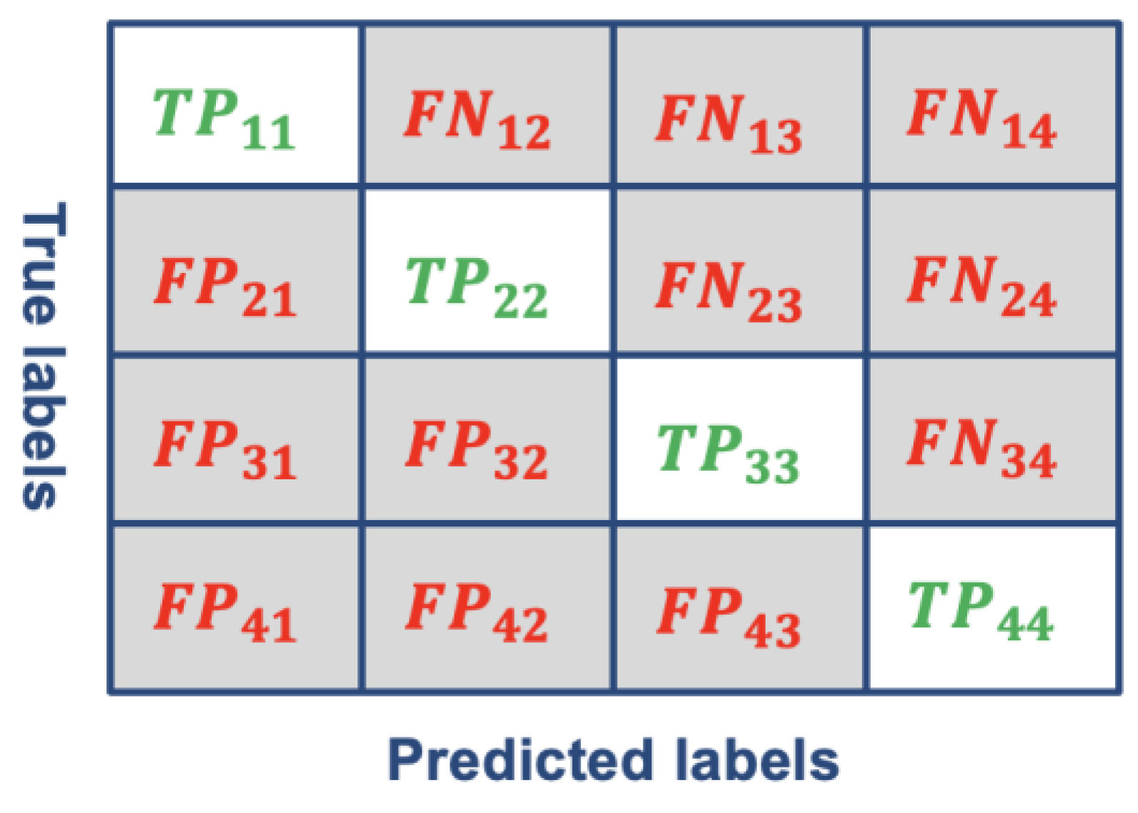
We evaluated the model performance using four standard metrics: accuracy, precision, recall, and F1-macro [60]. Accuracy measures the proportion of correct predictions, including both true positives (TP) and true negatives (TN), out of all predictions, as defined in Eq. (7). It provides an overall assessment of the model’s correctness. Precision () quantifies the proportion of correctly predicted positive instances among all instances predicted as positive, as shown in Eq. (8). It is particularly important when the cost of false positives (FP) is high. Recall () measures the proportion of correctly predicted positive instances among all actual positive instances, as defined in Eq. (9). It becomes critical when the cost of false negatives (FN) is high. The F1-macro score provides a balanced evaluation by considering both precision and recall across multiple classes, as expressed in Eq. (10). It represents the harmonic mean of precision and recall, offering a single comprehensive measure of the model’s classification performance.
Figure 9.
Confusion matrix.
5. Results and Discussion
The results of benchmark and experimental setup showed different results as shown in Table 7 and Figure 10. In our experiment setup dataset, CNN-S performs the best by achieving over 99% F1 score, followed by LSTM-F as the second-best performer by achieving 93% average accuracy. In comparison, LSTM-F achieved the best performance with an F1 score exceeding 99%, followed by CNN-S as the second-best with F1 score of 91%.
Table 7.
Accuracy and F1 macro of all experimental results.
| Dataset 1 (Acc. / F1) |
Dataset 2 (Acc. / F1) |
Dataset 3 (Acc. / F1) |
Dataset 4 (Acc. / F1) |
Exp. A (Acc. / F1) |
Exp. B (Acc. / F1) |
|
|---|---|---|---|---|---|---|
| CNN | 0.92 / 0.92 | 0.91 / 0.91 | 0.91 / 0.90 | 0.92 / 0.92 | 0.99 / 0.99 | 0.99 / 0.99 |
| LSTM-T | 0.80 / 0.79 | 0.80 / 0.80 | 0.81 / 0.81 | 0.80 / 0.80 | 0.90 / 0.90 | 0.78 / 0.76 |
| LSTM-F | 0.99 / 0.99 | 0.99 / 0.99 | 0.99 / 0.99 | 1.0 / 1.0 | 0.90 / 0.90 | 0.96 / 0.96 |
Upon completion of training, the CNN outputs were averaged pixel-by-pixel to visualize the physical information most critical for classification and to interpret performance differences from the perspective of the network architecture. Figure 11 presents the heatmaps corresponding to the four bearings from Experiments A and B. High-intensity pixels indicate regions where the image patterns associated with specific fault modes are more prominently represented.
In our experimental dataset, the frequency ranges exhibit strong activation across all time intervals for all four bearings. Notably, higher-frequency components were inconsistently excited in all three fault-bearing cases, irrespective of rotational speed or fault frequency, unlike the patterns observed in Figure 5 and Figure 6. This phenomenon likely results from the rough surface texture of the defective regions, which generates irregular high-frequency components and elevated energy responses. Moreover, as shown in Figure 11(e)–(l), the CNN consistently focused on relatively high-frequency regions, suggesting that these ranges play an important role in fault discrimination. In Figure 5 and Figure 6, most fault-related energy is concentrated below 50 Hz, implying that the fault patterns would be primarily captured in the low-frequency range when using STFT. However, the CNN representations in Figure 11 indicate that not only frequencies below 50 Hz but also high-frequency regions above 200 Hz are significant for classification.
In contrast, the benchmark dataset exhibits clearer distinctions in frequency trends across fault modes (OF, IF, and RF) [61], as shown in Figure 11(a)–(d). The rotational characteristics of the bearings and motors are more prominently captured in these representations. Furthermore, the CNN representations derived from the benchmark dataset display noticeable temporal variations compared to those from our experimental dataset. This observation suggests that when fault-related frequency characteristics are distinctly defined, classification performance can be enhanced by emphasizing specific frequency bands rather than modeling the entire time–frequency complexity.
To further investigate the physical significance of the learned representations, we applied transposed convolution to the extracted feature maps to restore them to the original image dimensions. Figure 12 and Figure 13 show the reconstructed STFT-based heatmaps and their corresponding magnified views, respectively. In Figure 12 and Figure 13(e)–(l), certain frequency patterns are observed to recur periodically over time, indicating that the CNN successfully captured repetitive time–frequency features associated with bearing faults. In contrast, as shown in Figure 12 and Figure 13(a)–(d), the benchmark dataset, which exhibits more distinct frequency characteristics, did not produce such consistent temporal recurrences. This difference arises because the benchmark dataset represents more severe fault conditions, leading to clear frequency distinctions among fault types. Meanwhile, our experimental dataset, which involves milder defects, lacks such clearly separable frequency features, thereby necessitating the CNN to learn more complex joint time–frequency representations.
The difference in representation between the two datasets is particularly significant because CNNs fundamentally rely on repetitive spatial patterns within images. When consistent feature patterns corresponding to specific labels are absent, the model’s training stability tends to decrease, as also reflected in Table 7. LSTM models, on the other hand, predict labels by processing the current sequence in conjunction with all preceding sequences. Owing to their recurrent structure, LSTMs must extract distinguishable representations at consistent temporal or spectral indices to maintain stable learning. To examine this behavior, we analyzed both the input features and the output representations of the LSTM models to determine whether they consistently captured discriminative patterns. Figure 14 visualizes the average output activations of LSTM cells across the entire training dataset. A higher average activation at a specific index (time or frequency) indicates that the model identified that index as containing critical information. As shown in Figure 14(a), LSTM models trained on datasets yielding superior performance exhibit clearly distinguishable index activations, suggesting that the model successfully learned meaningful sequential dependencies. Conversely, in LSTM models that underperformed relative to CNN, the activation distributions lack such distinct features. This difference is particularly evident in the time-domain model (LSTM-T). Because LSTMs make predictions based on both current and previous index values, datasets that do not exhibit consistent sequential relationships hinder effective learning. This observation is supported by the performance trends summarized in Figure 14 and Table 7.
Considering the results of CNN-S, LSTM-T, and LSTM-F, we observed that when the modal frequency characteristics and time-domain vibration behaviors were highly similar—as shown in Figure 3, Figure 5, and Figure 6—the extracted representations became ambiguous and difficult to discriminate, as illustrated in the second and third rows of Figure 12 and Figure 13 and the second and third columns of Figure 14. Consequently, all three methods required a relatively large amount of training data (approximately 400 samples) to achieve satisfactory performance, with CNN-S ultimately producing the most reliable results. In contrast, for major defects, as reported in [57] and [61], the frequency and time–frequency characteristics were clearly distinguishable. Under such conditions, even a small amount of training data (around 40 samples) was sufficient to achieve accurate predictions, and the LSTM-F model demonstrated the best performance. The extracted representations in this case exhibited well-separated vector distributions, as seen in Figure 12 and Figure 13 (a)–(d) and Figure 14 (a) and (d). However, the LSTM-T model consistently failed to yield stable or distinctive representations, resulting in the lowest accuracy among the three approaches. Therefore, the CNN-S approach is more appropriate for minor defect scenarios, whereas the LSTM-F model is preferable for major defect conditions.
6. Conclusions
This study conducted a fundamental investigation into the performance of CNN and LSTM models for bearing fault diagnosis through a purposefully simplified and interpretable experimental framework. By utilizing both a widely adopted benchmark dataset (CWRU) and a custom-designed low-speed bearing dataset, we demonstrated that the optimal model selection is critically dependent on the nature of the frequency-domain characteristics present in the vibration data.
The key finding of our work is that the superiority of a given architecture is not universal but is dictated by the data separability in the frequency domain. LSTM models, particularly when fed with frequency-domain handcrafted features (LSTM-F), excel in scenarios where bearing faults generate distinct and easily separable spectral signatures. This was clearly observed in the CWRU dataset, which contains significant faults. In contrast, CNN models processing STFT spectrograms (CNN-S) demonstrated superior performance when dealing with minor or incipient faults that do not produce clearly distinguishable frequency patterns, as evidenced by our experimental low-speed bearing dataset. The time-domain LSTM (LSTM-T) consistently underperformed in both scenarios, highlighting the importance of frequency-domain information for this task.
The simplified, single-layer architecture employed in this study was instrumental in enabling a transparent analysis of the learned representations. This design choice allowed us to directly attribute performance differences to the core learning mechanisms of each model: LSTMs’ ability to capture sequential dependencies in well-defined feature sequences versus CNNs’ strength in identifying complex, local spatial patterns within time-frequency representations. The representation analysis provided clear evidence that LSTM-F relies on consistent, index-specific patterns, whereas CNN-S leverages more complex time-frequency interactions, making it more robust under low-separability conditions.
Based on these findings, we propose a practical guideline for model selection in industrial applications: LSTM-F is the preferred choice for diagnosing severe faults with distinct spectral features, while CNN-S is more effective for detecting minor defects or for systems exhibiting complex and weakly discriminative frequency behavior.
For future work, the fundamental insights gained from this controlled study should be validated and extended. A natural progression is to investigate whether the same performance trends and selection guidelines hold for more complex, state-of-the-art models such as deep convolutional networks and Transformer-based architectures. Furthermore, applying these guidelines to real-world, noisy industrial environments and exploring automated methods to assess dataset “frequency separability” for model selection would be valuable contributions to the field of predictive maintenance.
Author Contributions
Methodology, validation, investigation, data curation, and writing, J.-W.K.; conceptualization, data curation, writing-review & editing, funding acquisition , Jong-Hak Lee and Sung-Hyun Choi ; conceptualization, writing, supervision, project administration, K.-S.P. All authors have read and agreed to the published version of the manuscript.
Funding
Please add: This work was supported by the National Research Foundation of Korea (NRF) grant funded by the Korea government (MSIT) (No.RS-2025-00515526), by RF systems Co., Ltd (202510040001), and by the Gachon University research fund of 2023(GCU-202308090001).
Data Availability Statement
The data that support the findings of this study are available from the corresponding author upon reasonable request.
Conflicts of Interest
The authors declare no conflicts of interest.
References
- SKF, Slewing bearings. https://cdn.skfmediahub.skf.com/api/public/0901d196809590fe/pdf_preview_medium/0901d196809590fe_pdf_preview_medium.pdf (accessed 15 September 2005).
- NSK, Technical report. https://www.nsk.com/content/dam/nsk/common/catalogs/ctrgPdf/bearings/e728g.pdf (accessed October 2013).
- Wu, G.; Yan, T.; Yang, G.; Chai, H.; Cao, C. A review on rolling bearing fault signal detection methods based on different sensors. Sensors, 2022, 22, 8330. [Google Scholar] [CrossRef]
- Wang, F.; Liu, C.; Su, W.; Xue, Z.; Li, H.; Han, Q. Condition monitoring and fault diagnosis methods for low-speed and heavy-load slewing bearings: A literature review. Journal of Vibroengineering, 2017, 19, 3429–3444. [Google Scholar] [CrossRef]
- Jin, X.; Chen, Y.; Wang, L.; Han, H.; Chen, P. Failure prediction, monitoring and diagnosis methods for slewing bearings of large-scale wind turbine: A review. Measurement, 2021, 172, 108855. [Google Scholar] [CrossRef]
- Moodie, C. An investigation into the condition monitoring of large slow speed slew bearings. 2009.
- Jain, P.; Bhosle, S. Analysis of vibration signals caused by ball bearing defects using time-domain statistical indicators. International Journal of Advanced Technology and Engineering Exploration, 2022, 9, 700. [Google Scholar] [CrossRef]
- Lebold, M.; Mcclintic, K.; Campbell, R.; Byington, C.; Maynard, K. Review of vibration analysis methods for gearbox diagnostics and prognostics. In: Proceedings of the 54th meeting of the society for machinery failure prevention technology. Virginia Beach, VA, 2000. p. 16.
- Mcinerny, S.; Dai, Y. Basic vibration signal processing for bearing fault detection. IEEE Transactions on education, 2003, 46, 149–156. [Google Scholar] [CrossRef]
- Kiral, Z.; Karagulle, H. Vibration analysis of rolling element bearings with various defects under the action of an unbalanced force. Mechanical systems and signal processing, 2006, 20, 1967–1991. [Google Scholar] [CrossRef]
- Ocak, H.; Loparo, K. Estimation of the running speed and bearing defect frequencies of an induction motor from vibration data. Mechanical systems and signal processing, 2004, 18, 515–533. [Google Scholar] [CrossRef]
- Yang, H.; Mathew, J.; Ma, L. Vibration feature extraction techniques for fault diagnosis of rotating machinery: a literature survey. In: Asia-pacific vibration conference. 2003. p. 801-807.
- Saruhan, H.; Saridemir, S.; Qicek, A.; Uygur, I. Vibration analysis of rolling element bearings defects. Journal of applied research and technology, 2014, 12, 384–395. [Google Scholar] [CrossRef]
- Kapangowda, N.; Krishna, H.; Vasanth, S.; Thammaiah, A. Internal combustion engine gearbox bearing fault prediction using J48 and random forest classifier. International Journal of Electrical & Computer Engineering (2088-8708), 2023, 13.4. [CrossRef]
- Knight, A.; Bertani, S. Mechanical fault detection in a medium-sized induction motor using stator current monitoring. IEEE Transactions on Energy Conversion 2005, 20, 753–760. [Google Scholar] [CrossRef]
- Caesarendra, W. Vibration and acoustic emission-based condition monitoring and prognostic methods for very low speed slew bearing.
- Caesarendra, W.; Kosasih, P.; Tieu, A.; Moodie, C.; Choi, B. Condition monitoring of naturally damaged slow speed slewing bearing based on ensemble empirical mode decomposition. Journal of Mechanical Science and Technology, 2013, 27, 2253–2262. [Google Scholar] [CrossRef]
- Caesarendra, W.; Park, J.; Kosasih, P.; Choi, B. Condition monitoring of low speed slewing bearings based on ensemble empirical mode decomposition method. Transactions of the Korean Society for Noise and Vibration Engineering, 2013, 23, 131–143. [Google Scholar] [CrossRef]
- Žvokelj, M.; Zupan, S.; Prebil, I. Multivariate and multiscale monitoring of large-size low-speed bearings using ensemble empirical mode decomposition method combined with principal component analysis. Mechanical Systems and Signal Processing, 2010, 24, 1049–1067. [Google Scholar] [CrossRef]
- Han, T.; Liu, Q.; Zhang, L.; Tan, A. Fault feature extraction of low speed roller bearing based on Teager energy operator and CEEMD. Measurement, 2019, 138, 400–408. [Google Scholar] [CrossRef]
- Caesarendra, W.; Kosasih, B.; Tieu, A.; Moodie, C. Circular domain features based condition monitoring for low speed slewing bearing. Mechanical Systems and Signal Processing, 2014, 45, 114–138. [Google Scholar] [CrossRef]
- Caesarendra, W.; Kosasih, B.; Tieu, A.; Moodie, C. Application of the largest Lyapunov exponent algorithm for feature extraction in low speed slew bearing condition monitoring. Mechanical Systems and Signal Processing, 2015, 50, 116–138. [Google Scholar] [CrossRef]
- Luo, P.; Hu, Y. (2019). research on rolling bearing fault identification method based on LSTM neural network. In IOP Conference Series: Materials Science and Engineering (Vol. 542, No. 1, p. 012048). IOP Publishing. [CrossRef]
- Wang, J.; Mo, Z.; Zhang, H.; Miao, Q. A deep learning method for bearing fault diagnosis based on time-frequency image. IEEE Access 2019, 7, 42373–42383. [Google Scholar] [CrossRef]
- Avci, O.; Abdeliaber, O.; Kiranyaz, S.; Hussein, M.; Gabbouj, M.; Inman, D. A review of vibration-based damage detection in civil structures: From traditional methods to Machine Learning and Deep Learning applications. Mechanical systems and signal processing, 2021, 147, 107077. [Google Scholar] [CrossRef]
- An, Y.; Zhang, K.; Liu, Q.; Chai, Y.; Huang, X. Rolling bearing fault diagnosis method base on periodic sparse attention and LSTM. IEEE Sensors Journal, 2022, 22, 12044–12053. [Google Scholar] [CrossRef]
- Gu, K.; Zhang, Y.; Liu, X.; Li, H.; Ren, M. DWT-LSTM-based fault diagnosis of rolling bearings with multi-sensors. Electronics, 2021, 10, 2076. [Google Scholar] [CrossRef]
- Xueyi, L.; Kaiyu, S.; Qiushi, H.; Xiangkai, W.; Zhijie, X. (2023). Research on fault diagnosis of highway Bi-LSTM based on attention mechanism. Eksploatacja i Niezawodność-maintennace and reliability, 25(2).
- Li, C.; Xu, J.; Xing, J. A Frequency Feature Extraction Method Based on Convolutional Neural Network for Recognition of Incipient Fault. IEEE Sensors Journal, 2023. [CrossRef]
- Zhang, Q.; Deng, L. An intelligent fault diagnosis method of rolling bearings based on short-time Fourier transform and convolutional neural network. Journal of Failure Analysis and Prevention, 2023, 23, 795–811. [Google Scholar] [CrossRef]
- Yang, S.; Yang, P.; Yu, H.; Bai, J.; Feng, W.; Su, Y.; Si, Y. A 2DCNN-RF model for offshore wind turbine high-speed bearing-fault diagnosis under noisy environment. Energies 2022, 15, 3340. [Google Scholar] [CrossRef]
- Bengio, Y.; Courville, A.; Vincent, P. Representation learning: A review and new perspectives. IEEE transactions on pattern analysis and machine intelligence, 2013, 35, 1798–1828. [Google Scholar] [CrossRef] [PubMed]
- Alzawi, S.; Mohammed, T.; Albawi, S. Understanding of a convolutional neural network. In: 2017 international conference on engineering and technology (ICET). Ieee, 2017. p. 1-6.
- Toma, R.; Piltan, F.; Im, K.; Shon, D.; Yoon, T.; Yoo, D.; Kim, J. A bearing fault classification framework based on image encoding techniques and a convolutional neural network under different operating conditions. Sensors 2022, 22, 4881. [Google Scholar] [CrossRef]
- Pham, M.; Kim, J.; Kim, C. 2D CNN-based multi-output diagnosis for compound bearing faults under variable rotational speeds. Machines, 2021, 9, 199. [Google Scholar] [CrossRef]
- Alzubaidi, L.; Zhang, J.; Humaidi, A.; Al-Dujaili, A.; Duan, Y.; Al-Shamma, O.; Santamaria, J.; Fadhel, M.; Al-Amidie, M.; Farhan, L. Review of deep learning: Concepts, CNN architectures, challenges, applications, future directions. Journal of big Data, 2021, 8, 1–74. [Google Scholar] [CrossRef]
- Yosinski, J.; Clune, J.; Nguyen, A.; Lipson, H.; Fuches, T. Understanding Neural Networks Through Deep Visualization. [CrossRef]
- Zeiler, M.; Fergus, R. Visualizing and understanding convolutional networks. In: Computer Vision–ECCV 2014: 13th European Conference, Zurich, Switzerland, September 6-12, 2014, Proceedings, Part I 13. Springer International Publishing, 2014. p. 818-833. [CrossRef]
- Protas, E.; Bratti, J.; Gaya, J.; Drews, P.; Botelho, S. Visualization methods for image transformation convolutional neural networks. IEEE Transactions on Neural Networks and Learning Systems, 2018, 30, 2231–2243. [Google Scholar] [CrossRef] [PubMed]
- Rao, S. Mechanical vibrations. 2001.
- Sundararajan, D. The discrete Fourier transform: theory, algorithms and applications. World Scientific, 2001.
- Allen, J.; Rabiner, L. A unified approach to short-time Fourier analysis and synthesis. Proceedings of the IEEE, 1977, 65, 1558–1564. [Google Scholar] [CrossRef]
- Wang, B.; Feng, G.; Huo, D.; Kang, Y. A bearing fault diagnosis method based on spectrum map information fusion and convolutional neural network. Processes, 2022, 10, 1426. [Google Scholar] [CrossRef]
- Hochreiter, S.; Schmidhuber, J. Long short-term memory. Neural computation, 1997, 9, 1735–1780. [Google Scholar] [CrossRef] [PubMed]
- Staudemeyer, R.; Morris, E. Understanding LSTM--a tutorial into long short-term memory recurrent neural networks. arXiv preprint arXiv:1909.09586, 2019. [CrossRef]
- Zargar, S. Introduction to sequence learning models: RNN, LSTM, GRU. Department of Mechanical and Aerospace Engineering, North Carolina State University, Raleigh, North Carolina, 2021, 27606.
- Ptotić, M.; Stojanvić, M.; Popović, P. A Review of Machine Learning Methods for Long-Term Time Series Prediction. In: 2022 57th International Scientific Conference on Information, Communication and Energy Systems and Technologies (ICEST). IEEE, 2022. p. 1-4. [CrossRef]
- Song, W.; Gao, C.; Zhao Y.; Zhao Y. A time series data filling method based on LSTM—Taking the stem moisture as an example. Sensors, 2020, 20.18: 5045. [CrossRef]
- Cai, C.; Tao, Y.; Zhu, T.; Deng, Z. Short-term load forecasting based on deep learning bidirectional LSTM neural network. Applied Sciences, 2021, 11.17: 8129. [CrossRef]
- Park, S.; Park, K. A pre-trained model selection for transfer learning of remaining useful life prediction of grinding wheel. Journal of Intelligent Manufacturing, 2023, 1-18. [CrossRef]
- Caesarendra, W.; Tjahjowidodo, T. A review of feature extraction methods in vibration-based condition monitoring and its application for degradation trend estimation of low-speed slew bearing. Machines, 2017, 5.4: 21. [CrossRef]
- Case Western Reserve University Bearing Dataset, https://engineering.case.edu/bearingdatacenter.
- Pietrzak, P.; Wolkiesicz, M. Stator Winding Fault Detection of Permanent Magnet Synchronous Motors Based on the Short-Time Fourier Transform. Power Electronics and Drives, 2022, 7.1: 112-133.
- Ruiz, J.; Rosero, J.; Espinosa, A.; Romeral, L. Detection of demagnetization faults in permanent-magnet synchronous motors under nonstationary conditions. IEEE Transactions on Magnetics, 2009, 45.7: 2961-2969. [CrossRef]
- Rosero, J.; Ortega, J.; Urresty, J.; Ca ́rdenas, J.; Romeral, L. Stator short circuits detection in PMSM by means of higher order spectral analysis (HOSA). In: 2009 Twenty-Fourth Annual IEEE Applied Power Electronics Conference and Exposition. IEEE, 2009. p. 964-969. [CrossRef]
- Belbali, A.; Makhloufi, S.; Kadri, A.; Abdallah, L.; Seddik, Z. Mathematical Modelling of a 3-Phase Induction Motor. 2023.
- Smith, W.; Randall, R. Rolling element bearing diagnostics using the Case Western Reserve University data: A benchmark study. Mechanical systems and signal processing, 2015, 64: 100-131. [CrossRef]
- Mishra, C.; Samantaray, A.; Chakraborty, G. Ball bearing defect models: A study of simulated and experimental fault signatures. Journal of Sound and Vibration, 2017, 400: 86-112. [CrossRef]
- Erhan, D.; Bengio, Y.; Courvill, A.; Vincent, P. Visualizing higher-layer features of a deep network. University of Montreal, 2009, 1341.3: 1.
- Grandini, M.; Bagli, E.; Visani, G. Metrics for multi-class classification: an overview. arXiv preprint arXiv:2008.05756, 2020. [CrossRef]
- Yoo, Y.; Jo H.; Ban S. Lite and efficient deep learning model for bearing fault diagnosis using the CWRU dataset. Sensors, 2023, 23.6: 3157. [CrossRef]
Figure 1.
Experimental setup: (a) Test rig (b) Motor driver and PC (c) Oscilloscope and hard disk.
Figure 2.
Slightly defected bearings’ component: (a) Outer race fault (b) Inner race fault (c) Rolling element fault.
Figure 2.
Slightly defected bearings’ component: (a) Outer race fault (b) Inner race fault (c) Rolling element fault.
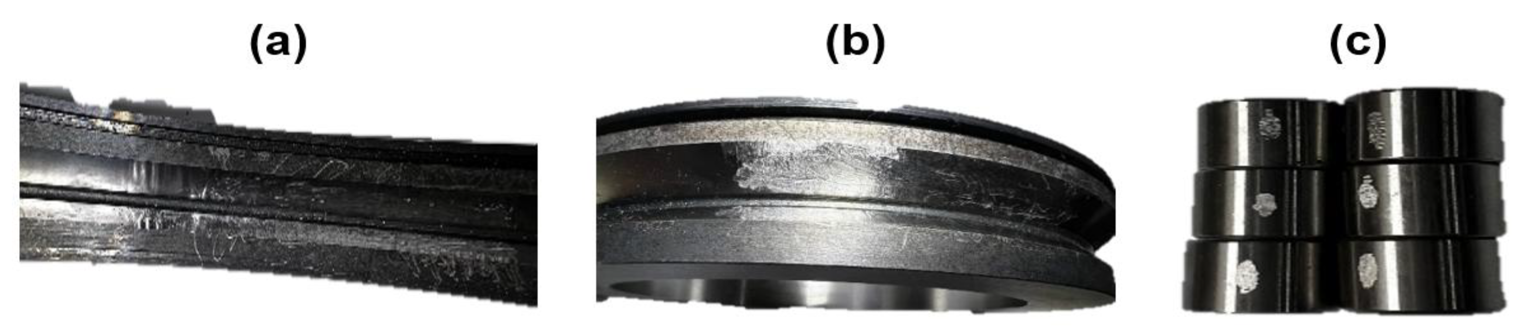
Figure 3.
Samples of acquired vibration signals of 5 RPM at axial direction: in order from the top, the raw vibration signal, the spectral signal and the spectral signal in the frequency range of 0 to 10 Hz: (a) Normal (b) Outer race fault (c) Inner race fault (d) Rolling element fault.
Figure 3.
Samples of acquired vibration signals of 5 RPM at axial direction: in order from the top, the raw vibration signal, the spectral signal and the spectral signal in the frequency range of 0 to 10 Hz: (a) Normal (b) Outer race fault (c) Inner race fault (d) Rolling element fault.
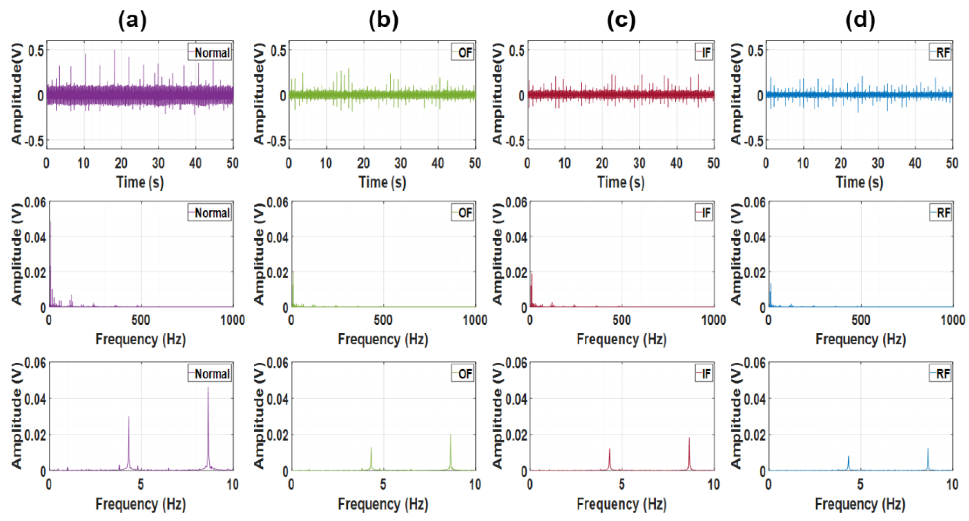
Figure 4.
Samples of acquired vibration signals of 20 RPM at radial direction: in order from the top, the raw vibration signal, the spectral signal and the spectral signal in the frequency range of 0 to 20 Hz: (a) Normal (b) Outer race fault (c) Inner race fault (d) Rolling element fault.
Figure 4.
Samples of acquired vibration signals of 20 RPM at radial direction: in order from the top, the raw vibration signal, the spectral signal and the spectral signal in the frequency range of 0 to 20 Hz: (a) Normal (b) Outer race fault (c) Inner race fault (d) Rolling element fault.
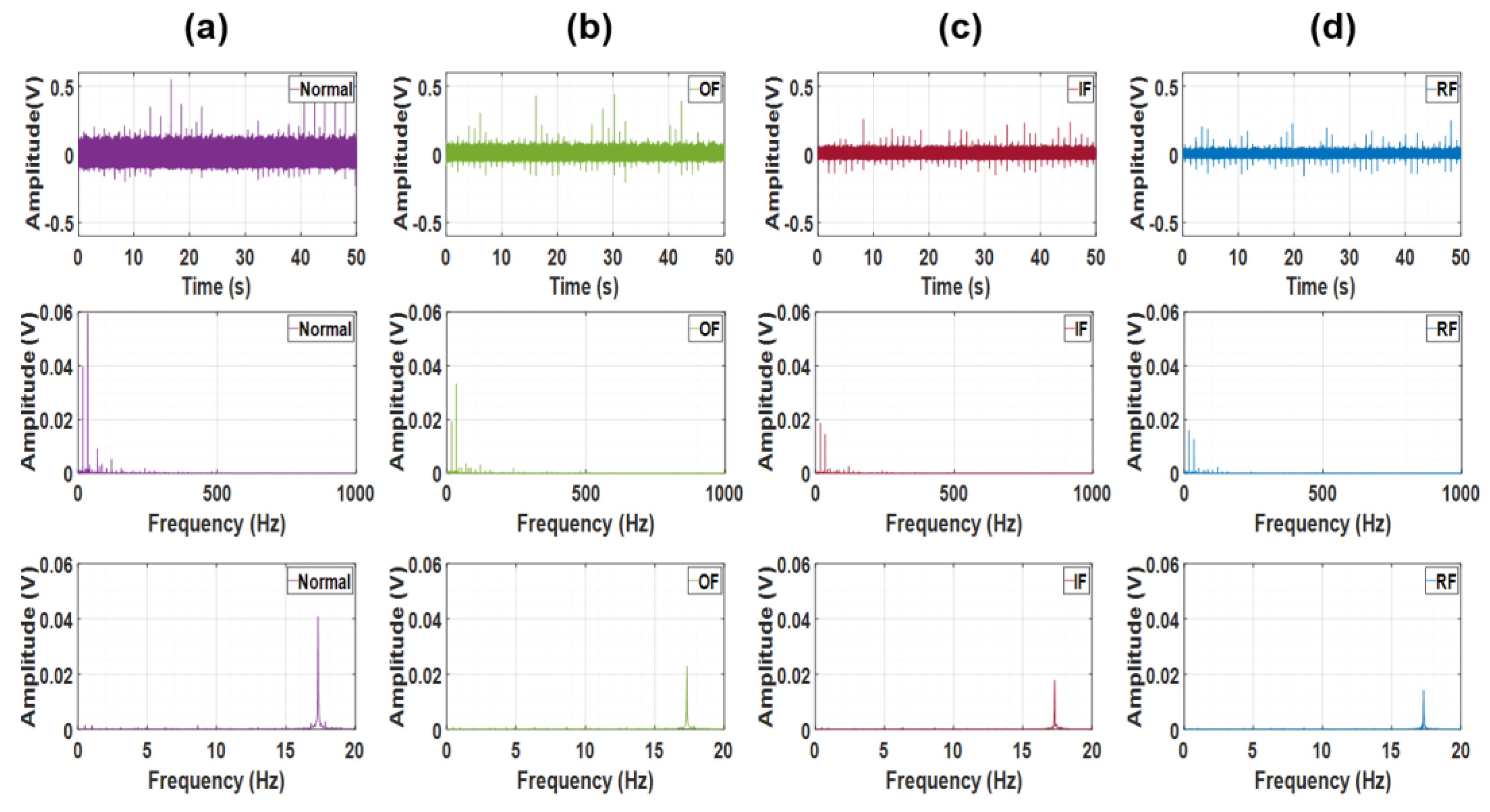
Figure 5.
Samples of STFT of Exp. B with selected parameters: first row is STFT result of radial and second is result of axial accelerometer: (a) Normal (b) Outer race fault (c) Inner race fault (d) Rolling element fault.
Figure 5.
Samples of STFT of Exp. B with selected parameters: first row is STFT result of radial and second is result of axial accelerometer: (a) Normal (b) Outer race fault (c) Inner race fault (d) Rolling element fault.
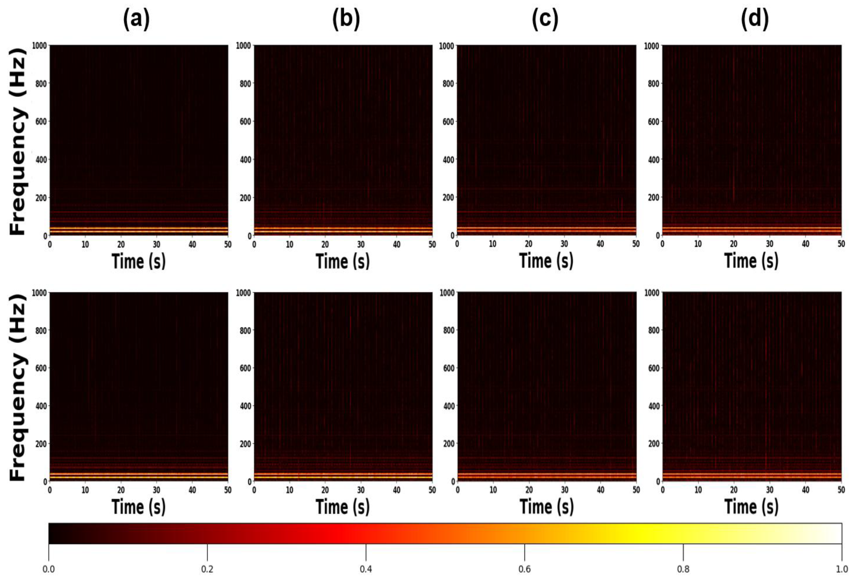
Figure 6.
Zoomed-in samples of STFT of Exp. B with selected parameters: first row is STFT result of radial and second is result of axial accelerometer: (a) Normal (b) Outer race fault (c) Inner race fault (d) Rolling element fault.
Figure 6.
Zoomed-in samples of STFT of Exp. B with selected parameters: first row is STFT result of radial and second is result of axial accelerometer: (a) Normal (b) Outer race fault (c) Inner race fault (d) Rolling element fault.
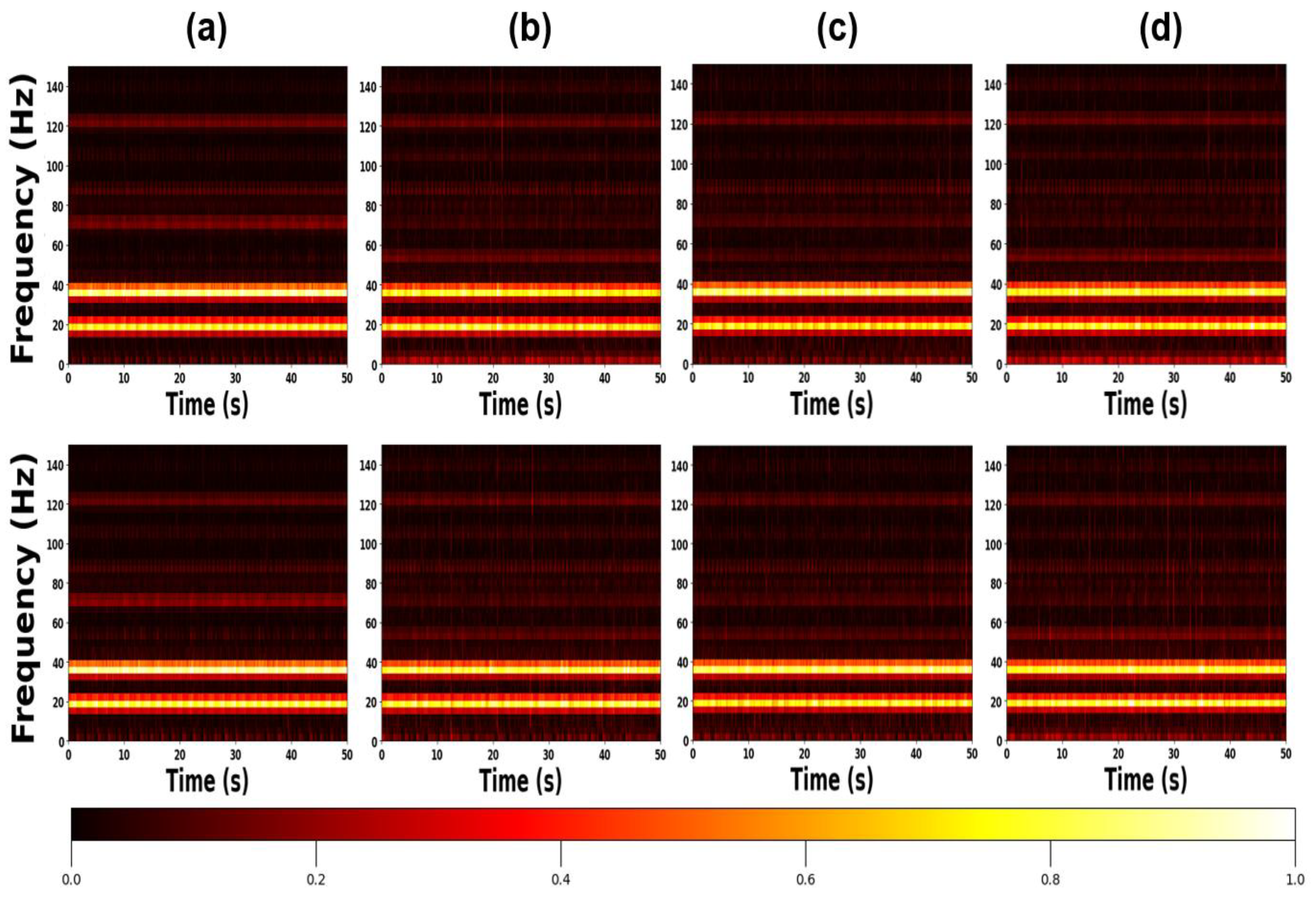
Figure 7.
Architecture of proposed basic CNN.
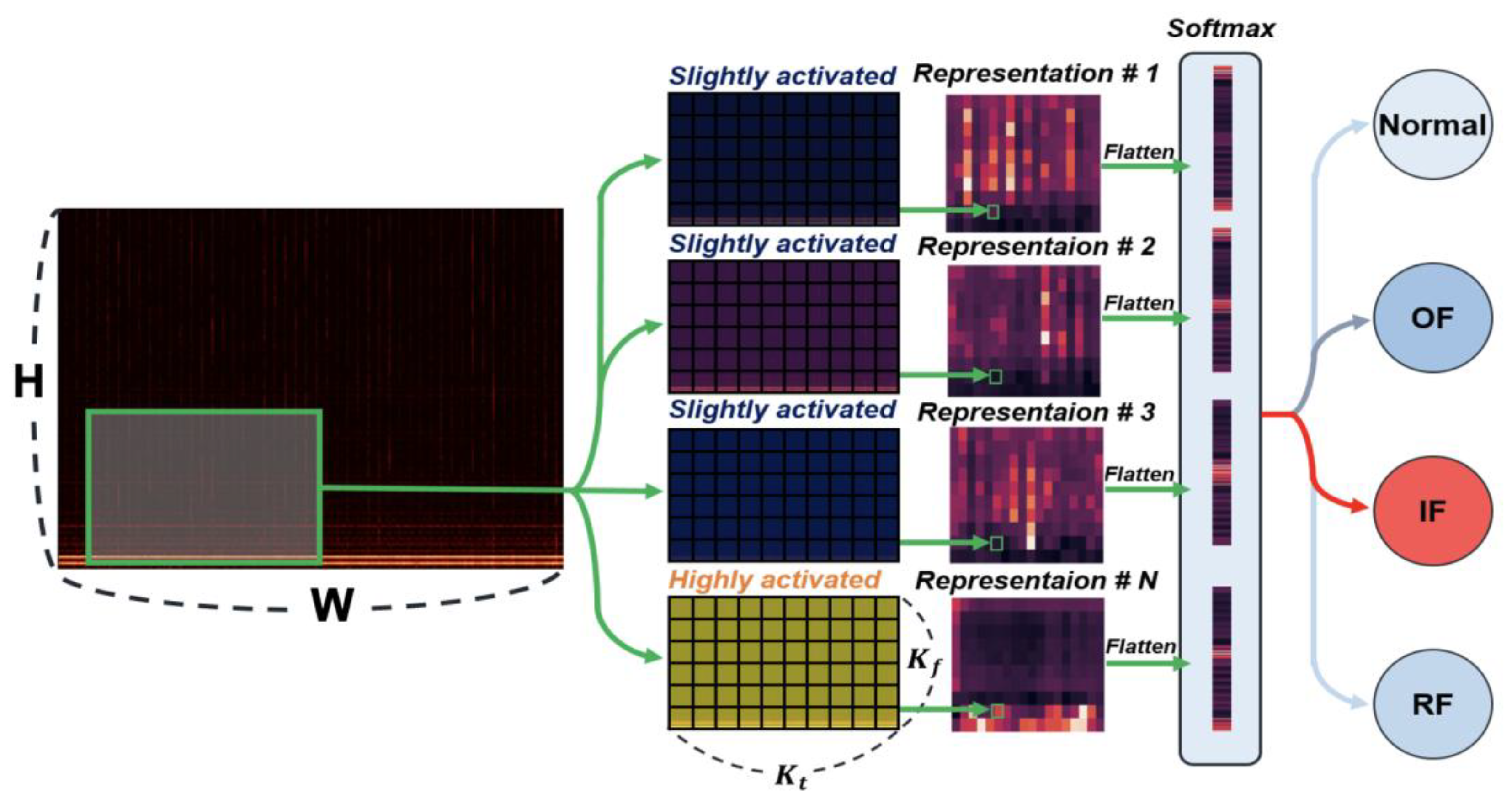
Figure 8.
Architecture of proposed basic LSTM.
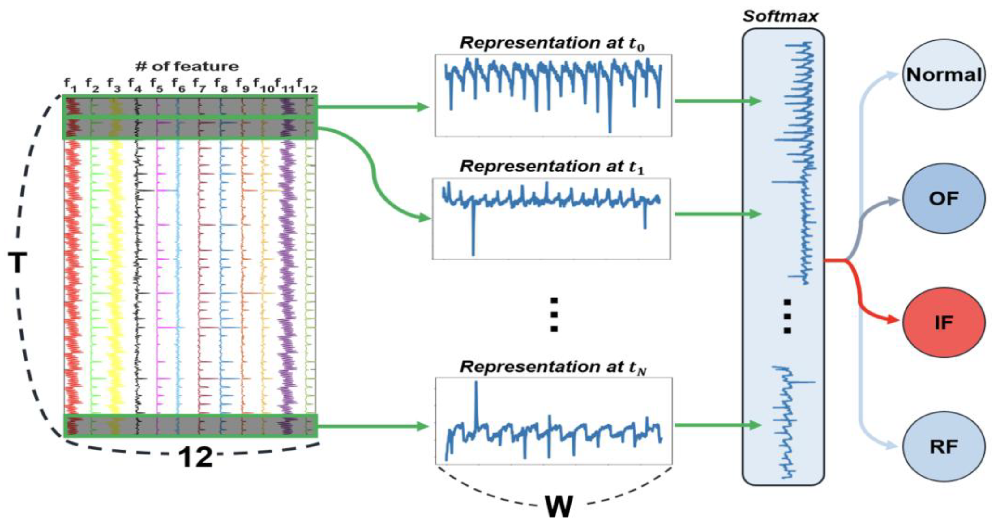
Figure 10.
Confusion matrices of CNN-based model: First row is result of experiment A and second is result of experiments B: (a) LSTM-T (b) LSTM-F (c) CNN-S.
Figure 10.
Confusion matrices of CNN-based model: First row is result of experiment A and second is result of experiments B: (a) LSTM-T (b) LSTM-F (c) CNN-S.
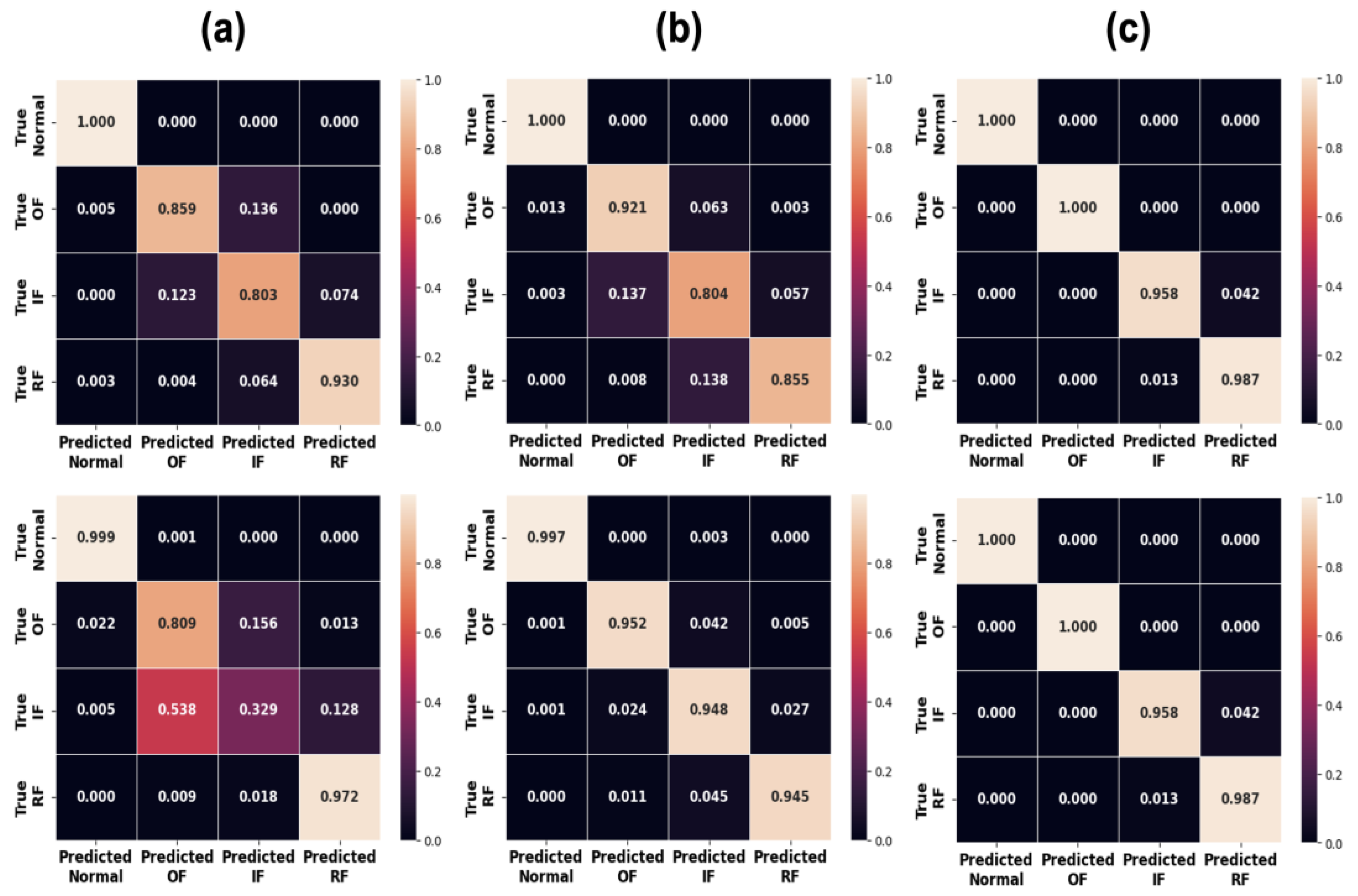
Figure 11.
Samples of summed feature maps: (a) CWRU Normal (b) CWRU outer fault (c) CWRU inner fault (d) CWRU rolling element fault (e) Exp. A Normal (f) Exp. A outer fault (g) Exp. A inner fault (h) Exp. A rolling element fault (i) Exp. B Normal (j) Exp. B outer fault (k) Exp. B inner fault (l) Exp. B rolling element fault.
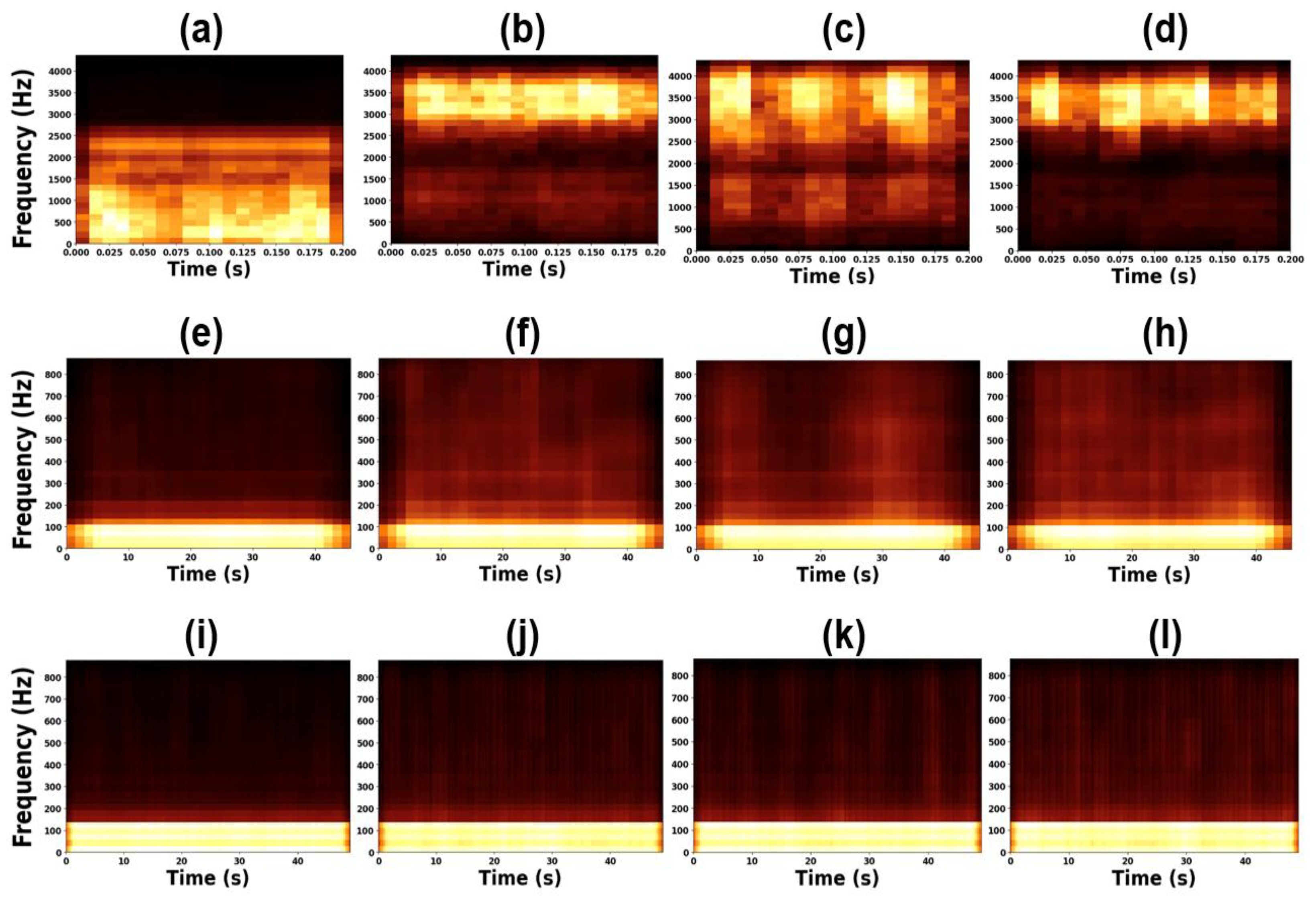
Figure 12.
Samples of deconvolution feature maps: (a) CWRU Normal (b) CWRU outer fault (c) CWRU inner fault (d) CWRU rolling element fault (e) Exp. A Normal (f) Exp. A outer fault (g) Exp. A inner fault (h) Exp. A rolling element fault (i) Exp. B Normal (j) Exp. B outer fault (k) Exp. B inner fault (l) Exp. B rolling element fault.
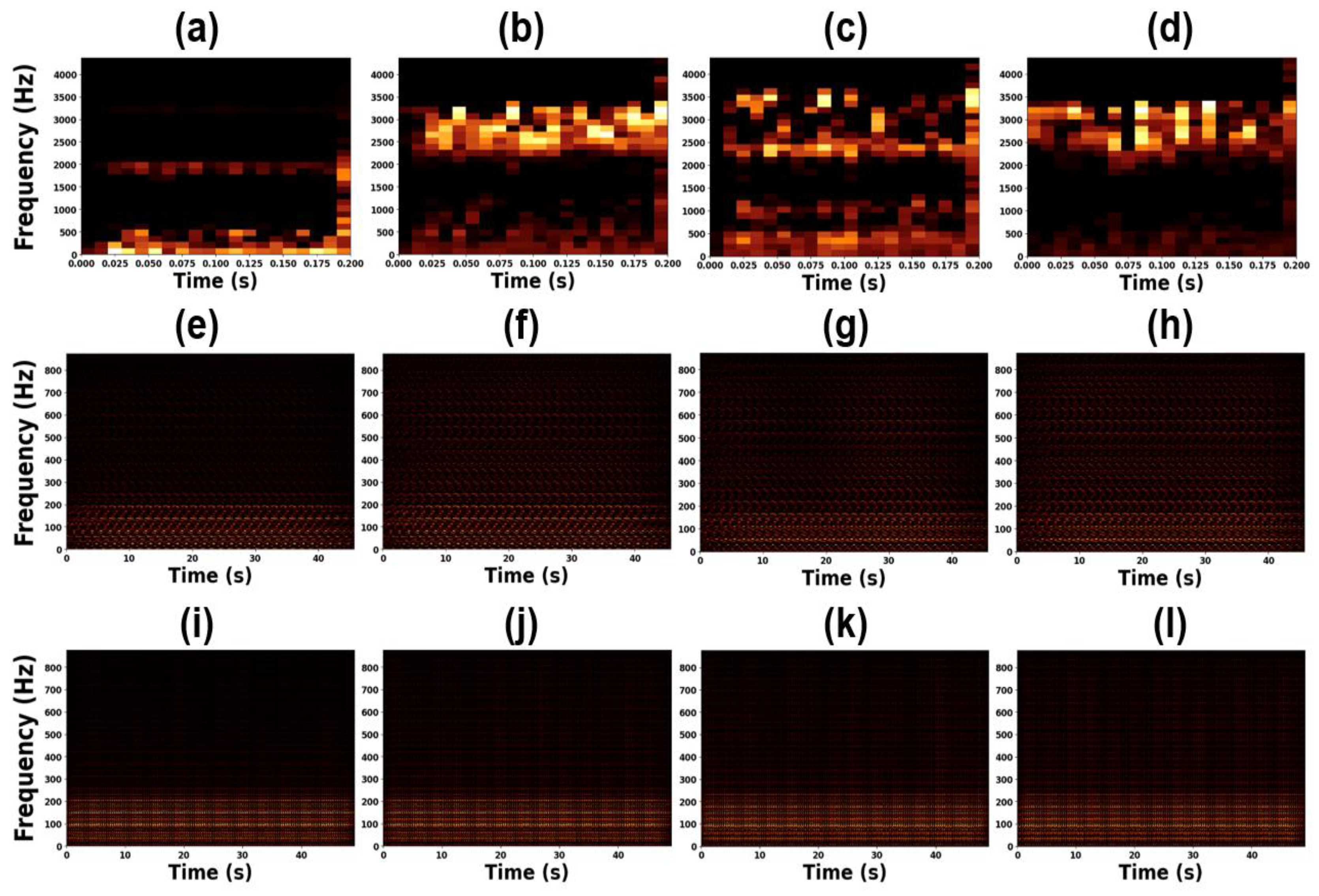
Figure 13.
Zoomed-in samples of deconvolution feature maps: (a) CWRU Normal (b) CWRU outer fault (c) CWRU inner fault (d) CWRU rolling element fault (e) Exp. A Normal (f) Exp. A outer fault (g) Exp. A inner fault (h) Exp. A rolling element fault (i) Exp. B Normal (j) Exp. B outer fault (k) Exp. B inner fault (l) Exp. B rolling element fault.
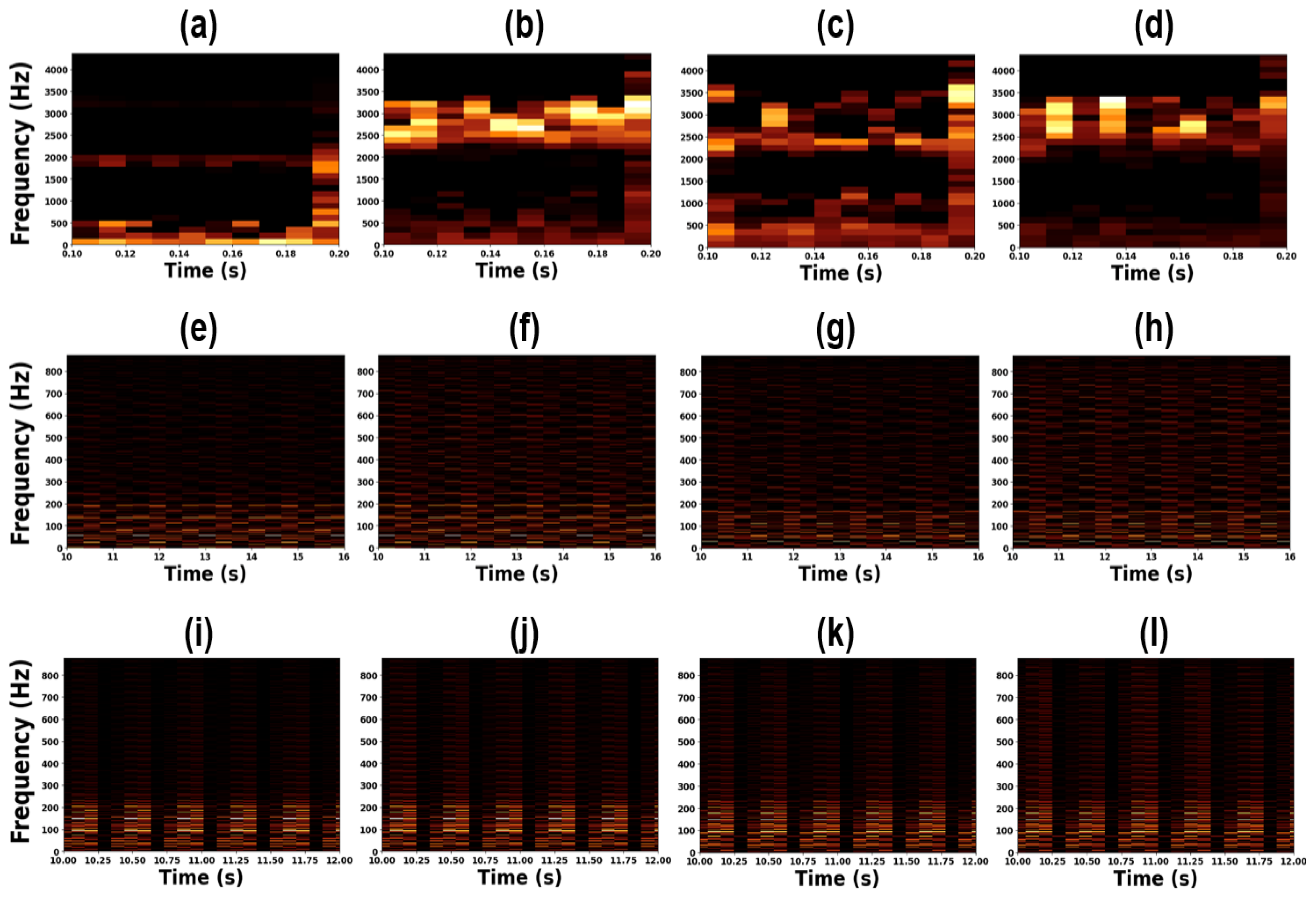
Figure 14.
Averaged LSTM’s outputs through time or frequency: (a) CWRU LSTM-F (b) Exp. A LSTM-F (c) Exp. B LSTM-F (d) CWRU LSTM-T (e) Exp. A LSTM-T (f) Exp. B LSTM-T.
Figure 14.
Averaged LSTM’s outputs through time or frequency: (a) CWRU LSTM-F (b) Exp. A LSTM-F (c) Exp. B LSTM-F (d) CWRU LSTM-T (e) Exp. A LSTM-T (f) Exp. B LSTM-T.
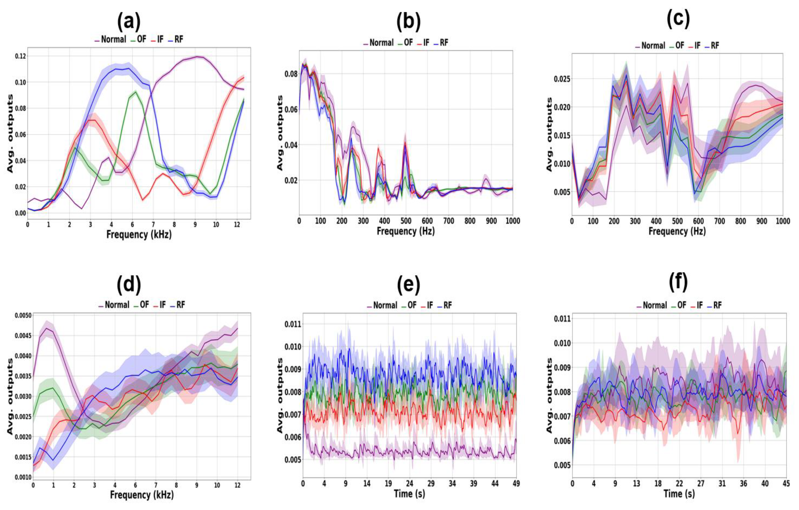
Table 2.
Case Western Reserve University dataset, divided by RPM conditions.
| Dataset | RPM | Failure mode | Training size |
Validation size |
Test size |
|---|---|---|---|---|---|
| Dataset 1 | 1730 | Normal, OF, IF and RF | 40 | 281 | 281 |
| Dataset 2 | 1750 | Normal, OF, IF and RF | 40 | 281 | 281 |
| Dataset 3 | 1773 | Normal, OF, IF and RF | 40 | 281 | 281 |
| Dataset 4 | 1797 | Normal, OF, IF and RF | 40 | 231 | 231 |
Table 3.
Experimental setup dataset, divided by RPM conditions.
| Dataset | RPM | Failure mode | Training size |
Validation size |
Test size |
|---|---|---|---|---|---|
| Exp. A | 5 | Normal, OF, IF and RF | 240 | 3,080 | 3,080 |
| Exp. B | 20 | Normal, OF, IF and RF | 240 | 3,080 | 3,080 |
Table 4.
Fault frequencies and preprocessing parameters.
| Dataset 1 |
Dataset 2 |
Dataset 3 |
Dataset 4 |
Exp. A | Exp. B | |
|---|---|---|---|---|---|---|
| Rolling element frequency | 135 Hz | 138 Hz | 139 Hz | 141 Hz | 1.6 Hz | 6.5 Hz |
| Outer pass frequency |
103 Hz | 105 Hz | 106 Hz | 107 Hz | 2.5 Hz | 9.8 Hz |
| Inner pass frequency |
155 Hz | 158 Hz | 160 Hz | 162 Hz | 2.6 Hz | 10.4 Hz |
| Selected | 70 | 70 | 70 | 70 | 688 | 190 |
| Selected | 90 | 90 | 90 | 90 | 2344 | 586 |
| Selected | 20 | 20 | 20 | 20 | 1656 | 396 |
Table 5.
Input sizes of preprocessed features.
| Exp. A STFT |
Exp. A handcrafted | Exp. B STFT |
Exp. B handcrafted | CWRU STFT |
CWRU handcrafted |
|
| Input size |
(1024, 128) | (128, 12) | (256, 512) | (512, 12) | (32, 32) | (32, 12) |
Table 6.
Kernel sizes, striding intervals and channels of CNN-based models.
| Exp. A | Exp. B | CWRU | |
|---|---|---|---|
| Kernel size (, , ) | (256, 16, 64) | (64, 31, 64) | (8, 5, 64) |
| Striding interval (, ) | (32, 4) | (8, 4) | (1, 1) |
| # of parameters | 262,208 | 127,040 | 2,624 |
Table 7.
Number of hidden units and parameters for LSTM-based models.
| Exp. A | Exp. B | CWRU | |
|---|---|---|---|
| # of hidden units | 250 | 172 | 20 |
| # of parameters | 263,000 | 127,008 | 2,640 |
Disclaimer/Publisher’s Note: The statements, opinions and data contained in all publications are solely those of the individual author(s) and contributor(s) and not of MDPI and/or the editor(s). MDPI and/or the editor(s) disclaim responsibility for any injury to people or property resulting from any ideas, methods, instructions or products referred to in the content. |
© 2025 by the authors. Licensee MDPI, Basel, Switzerland. This article is an open access article distributed under the terms and conditions of the Creative Commons Attribution (CC BY) license (http://creativecommons.org/licenses/by/4.0/).
Copyright: This open access article is published under a Creative Commons CC BY 4.0 license, which permit the free download, distribution, and reuse, provided that the author and preprint are cited in any reuse.


