
Submitted:
21 November 2025
Posted:
24 November 2025
You are already at the latest version
Abstract
Noise can substantially distort both chaotic and physiological dynamics, obscuring deterministic patterns and altering the apparent complexity of signals. Accurately identifying and characterizing such perturbations is essential for reliable analysis of dynamical and biomedical systems. This study combines complexity-based features with supervised learning to characterize and predict noise perturbations in time series data. Using two chaotic systems (Rössler and Lorenz) and synthetic electrocardiogram (ECG) signals, we generated controlled Gaussian, pink, and low-frequency noise of varying intensities and extracted a diverse set of 18 complexity metrics derived from both raw signals and phase-space embeddings. The analysis systematically evaluates how these metrics behave under different noise regimes and intensities and identifies the most discriminative features for noise classification tasks. Approximate Entropy, Mean Absolute Deviation, and Condition Number emerged as the strongest predictors for noise intensity, while Condition Number, Sample Entropy, and Permutation Entropy most effectively differentiated noise categories. Across all systems, the proposed framework reached an average accuracy of 99.9% for noise presence and type classification and 96.2% for noise intensity, significantly surpassing previously reported benchmarks for noise characterization in chaotic and physiological time series. These results demonstrate that complexity metrics encode both structural and statistical signatures of stochastic contamination.
Keywords:
machine learning
; feature extraction
; chaotic system
; catboost
; noise
; noise detection
; complexity metrics
; signal analysis
1. Introduction
Noise profoundly alters the apparent structure of a signal, masking deterministic dynamics and inflating perceived randomness. Understanding and quantifying these effects is essential for developing reliable diagnostic and predictive tools in dynamical and physiological systems [1]. For example, the detection of noise can warrant denoising [2] while different noise regimes demand distinct preprocessing strategies such as band-pass filtering for low-frequency drift [3]. Furthermore, understanding how different types and intensities of noise shape signal characteristics enables the identification of stable, discriminative features and fosters the development of robust signal analysis approaches [4].
Complexity metrics, such as entropy measures, fractal dimensions, and information-theoretic indices, offer a quantitative perspective for capturing transitions between order and stochasticity. In combination with machine learning (ML), it provides a powerful tool to discriminate complex trends and patterns for tabular and time series applications across domains [5,6,7,8,9].
Recent studies have provided empirical evidence that complexity metrics respond systematically to stochastic perturbations. Makowski et al. [10] compared fractal and entropy-based measures across multiple coloured noise regimes and noise intensities, showing that individual metrics exhibit distinct sensitivity profiles. Ricci and Politi [11] demonstrated that permutation entropy increases predictably with weak observational noise in chaotic systems, revealing a measurable relationship between entropy growth and noise amplitude. Likewise, Cuesta-Frau et al. [4] used statistical methods and entropy methods for signal classification while Sara Maria et al. Mariani et al. [12] used multiscale entropy and threshold-based or comparative analysis to differentiate between clean and noisy artifacts. These studies highlight that complexity metrics are influenced by both the type and the magnitude of noise. However, they remain largely descriptive and do not attempt to predict noise properties using these metrics. Moreover, while Makowski et al. [10] compared a broad range of metrics, the focus was methodological rather than predictive, leaving open the question of which metrics are most informative for distinguishing specific noise characteristics.
In parallel, research in biomedical signal processing has applied machine learning (ML) methods to detect and classify noise, particularly in electrocardiogram (ECG) and electroencephalogram (EEG) analysis. Hayn et al. [13] proposed an early quality-assessment framework using amplitude- and morphology-based heuristics to identify noisy segments. Kumar and Sharma [14] introduced a sparse signal decomposition technique that detects and classifies baseline wander, muscle artefacts, power-line interference, and white Gaussian noise. More recently, Holgado-Cuadrado et al. [15] and Monteiro et al. [16] employed supervised and deep learning models to assess clinical noise severity in long-term ECG monitoring, achieving high detection accuracy. While these studies confirm the suitability of ML for noise detection, they primarily rely on statistical, spectral features or the unprocessed signal. None of them explicitly combine ML with complexity-based feature representations, nor do they analyse the predictive capacity of complexity metrics under systematically varied noise conditions.
Beyond biomedical signals, hybrid studies linking complexity measures and ML remain rare. Boaretto et al. [17] trained a neural network on time series with coloured noise to estimate spectral exponents and to discriminate chaotic from stochastic dynamics using permutation entropy as input. This work demonstrated that ML can leverage complexity measures to infer dynamical properties, but it did not aim to classify distinct noise types or intensities. Consequently, there is a clear research gap at the intersection of (i) descriptive analyses of how noise influences complexity, and (ii) predictive ML models that use complexity features to identify and quantify noise.
In this work, we address this gap by integrating complexity metrics into ML-based noise prediction across both synthetic and physiological signals. Specifically, we evaluate how diverse complexity measures capture variations induced by different noise types (Gaussian, pink, low-frequency) and intensity levels. By training supervised classifiers on these metrics, we identify which measures are most discriminative for noise characterization and demonstrate their generalizability across dynamical and biomedical domains. The main idea and corresponding machine learning pipeline is depicted in Figure 1.
Overall, this study provides the following contributions:
- A unified framework combining complexity metrics and machine learning to predict multiple noise types and intensities in both chaotic and physiological signals.
- A comparative evaluation of diverse complexity measures to determine which metrics most effectively characterize stochastic perturbations.
- A quantitative analysis of noise scaling effects, extending previous descriptive studies to predictive, multi-intensity classification tasks.
This integration bridges theoretical and applied research on complexity and noise, offering new insights into how structured dynamics degrade under stochastic influences and establishing a generalizable approach for complexity-based noise prediction.
2. Materials and Methods
The methodological framework of this study follows a unified pipeline designed to evaluate the capacity of complexity-based metrics to detect and characterize different types and intensities of noise in dynamical and physiological systems. The approach integrates (i) phase space reconstruction, (ii) controlled noise perturbations, (iii) complexity feature extraction, (iv) supervised learning analysis, and (v) a post-hoc analysis of feature importance and distribution to assess the discriminative power and relative importance of these metrics across complex time series.
2.1. Data Sources and Signal Generation
To ensure generalizability across both theoretical and empirical systems, three distinct time series were analyzed. All systems were simulated with a uniform sequence length of 2,000 samples to maintain a consistent temporal resolution and comparable embedding structure across experiments.
- Rössler System – a continuous chaotic oscillator defined bynumerically integrated using a fourth-order Runge–Kutta solver (solve_ivp) around the nominal parameter set , , and . To enhance stochastic diversity between runs, each initiation incorporated controlled random perturbations in both system parameters and initial conditions. Specifically, a, b, and c were independently varied within of their nominal values by sampling from a uniform distribution, and the initial conditions were perturbed by adding Gaussian noise with zero mean and a standard deviation of 0.05 around the canonical state . Each simulation was run for 250 seconds with a fixed integration step of 0.1 seconds; the first 50 seconds were discarded to remove transient behavior, and the remaining 200 seconds were used for analysis, representing the steady-state attractor dynamics. An example with noise intensities of 0.3 can be seen in Figure 2.
- Lorenz System – a canonical chaotic attractor described bysimulated around the configuration , , and using the same numerical scheme. For each run, , , and were independently perturbed within of these nominal values, and the initial state was offset by Gaussian noise . Each run used a unique random seed determined by its run index to generate reproducible yet distinct realizations. The system was simulated for 250 seconds with a step size of 0.1 seconds, and the first 50 seconds were discarded so that only the steady-state portion of the attractor was analyzed. An example with noise intensity of 0.3 can be seen in the Appendix, Figure A1.
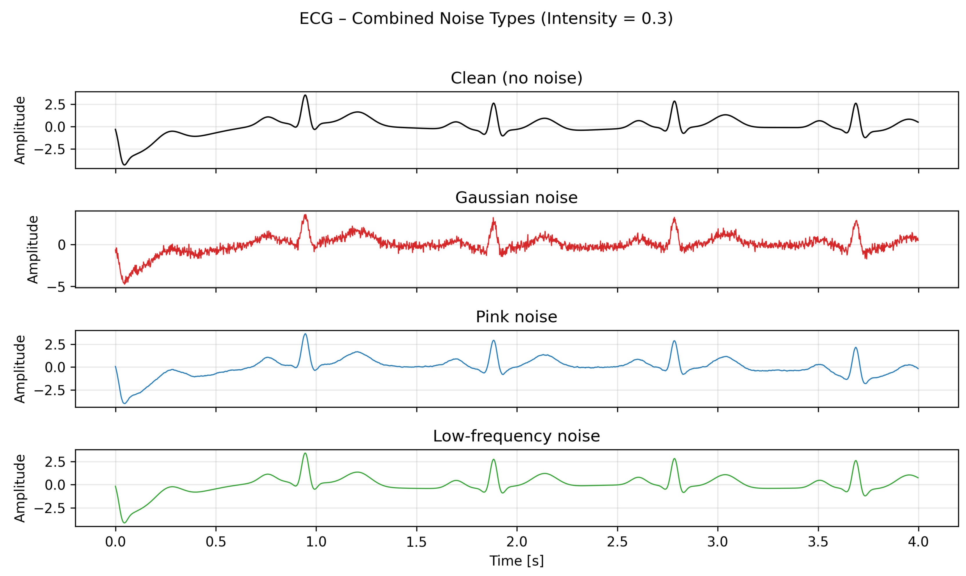
- Electrocardiogram (ECG) Signal – a physiological time series generated using the NeuroKit2 simulator to emulate quasi-periodic cardiac oscillations with natural physiological variability. Each ECG realization was generated with a unique random seed (run_id) that controlled two perturbation parameters: a randomly sampled heart rate and a phase shift applied to the waveform. The heart rate was drawn uniformly between 55 and 75 beats per minute, and a small temporal offset between and seconds was applied to emulate phase variability between cardiac cycles. Each signal was generated at 500 Hz for 4 seconds, cleaned using the built-in ECG processing pipeline, and padded or trimmed to a fixed length of 2,000 samples. These perturbations create physiologically plausible variability while preserving the general waveform morphology. An example with noise intensity of 0.3 can be seen in the Appendix, Figure A2.
2.2. Normalization and Noise Perturbation
All time series were first normalized using Z-score scaling to remove mean offsets and amplitude differences while preserving the underlying dynamical structure. Subsequently, controlled random perturbations were applied to the normalized signals to generate multiple variants under distinct noise configurations. Each perturbation process involved stochastic components. Gaussian and pink noise are random by design. The low-frequency modulation included randomized phase and frequency parameters to ensure temporal diversity between realizations. The complete set of noise configurations was defined as:
Each array specifies the relative intensity levels applied to the normalized signal, controlling the magnitude of the added perturbation. Three distinct types of noise were introduced:
- Gaussian noise () was generated as zero-mean white noise,where the standard deviation was scaled by the chosen intensity level.
- Pink noise () was produced with a power spectral density inversely proportional to frequency,representing temporally correlated stochastic fluctuations.
- Low-frequency interference () was modeled as a deterministic sinusoidal modulation,where A denotes the noise intensity, f was sampled uniformly from the interval , and the phase offset from the range . This introduces temporal misalignment of up to 20% of a full oscillation cycle between repeated realizations while maintaining consistent frequency and amplitude characteristics.
Each noise realization was generated with an independent random seed derived from the run index (random_seed 42 * run_id), ensuring that all perturbations were unique and reproducible. The same noise generation procedure was applied to the Lorenz, Rössler, and ECG systems to maintain methodological consistency and enable direct cross-system comparison.
2.3. Complexity Feature Extraction
A comprehensive set of 18 complexity metrics was computed to quantify the dynamical structure, regularity, and predictability of the underlying system. The extracted features were derived from both classical nonlinear time-series analysis and singular value decomposition (SVD)-based spectral metrics, providing complementary perspectives on temporal order and geometrical complexity within the embedded attractor.
Depending on the underlying metric, features were computed either directly on the raw time series or on the reconstructed phase-space embedding using the method of time-delayed coordinates [18]. I.e., given a discrete signal , we select an embedding dimension and a time delay . The embedded vectors are constructed as
with the constraint . The total number of available embedded vectors is therefore , and the valid indices are .
In all experiments, an embedding dimension of and a delay of sample were applied, providing a representation of the system’s dynamics while maintaining computational tractability, as computational costs of the presented analyses increase with increasing embedding dimensions. We note here that we are aware of characteristic embedding dimensions for, e.g., the Lorenz or the Rössler systems ( for both cases). However, in general, choosing a higher embedding dimension, though violating the topological identity with the actual system’s phase space, allows for expressive embeddings for the following noise analysis experiments.
A segment length of 300 samples (memory complexity = 300) was used to ensure temporal context for complexity estimation.
This distinction reflects the conceptual difference between metrics that capture temporal irregularity in the signal itself (e.g., entropy or scaling measures) and those that analyze the geometric structure of the attractor (e.g., SVD-based or derivative-based metrics). An overview of all computed features, their theoretical categories, and the corresponding data domains is summarized in Table 1.
All metrics were implemented in a modular Python pipeline based on NeuroKit2 [10] and custom analytical functions, ensuring consistent feature extraction and reproducibility across all three systems (Lorenz, Rössler, and ECG).
Entropy measures capture the degree of irregularity and information content in a signal. We computed:
-
Approximate Entropy (ApEn) [19], which quantifies the likelihood that similar patterns of observations remain similar at the next incremental step. Lower values indicate more regularity, while higher values imply greater unpredictability. Using the vectors from Equation 7, the distance between two embeddings and is defined through the maximum norm,For a given tolerance r, the quantityrepresents the fraction of embedded vectors that lie within a distance r of . The average logarithmic frequency of such recurrences isApproximate entropy is defined by comparing recurrence statistics for embedding dimensions and . Using the same delay , one computes and from their respective embedded vectors. The approximate entropy is thenThe quantity measures how often patterns of length repeat within a tolerance r, while summarizes this information across the entire trajectory. The difference quantifies how rapidly pattern similarity deteriorates when extending the embedding from dimension to . Larger values indicate lower regularity and weaker pattern persistence, whereas smaller values indicate more repetitive structure. The embedding dimension specifies the pattern length under consideration, and the delay determines the temporal spacing of the coordinates in accordance with Takens’ reconstruction framework.
-
Sample Entropy (SampEn) [20], a refinement of ApEn that removes self-matches and provides a more stable estimate for finite and noisy data. Using the same embedded vectors from Equation 7, the distance between two embeddings is again defined byFor a tolerance r, define B as the number of pairs with such that the distance between embeddings of dimension satisfiesand define A analogously as the number of pairs for embeddings of dimension , constructed with the same delay . Sample entropy is thenThe quantity B represents the number of pattern matches of length , while A counts those that persist when extending the embedding to dimension . Excluding self-matches avoids bias present in ApEn and leads to a more reliable estimate of the conditional likelihood that similar patterns remain similar at the next step. Lower values indicate higher regularity and stronger pattern recurrence.
- Permutation Entropy (PE) [21], which evaluates the diversity of ordinal patterns in the original time series. In this work, permutation entropy was computed using the NeuroKit2 implementation, which returns a normalized entropy measure. For each index i, the ordering of the consecutive values defines an ordinal pattern of order m. Let denote the relative frequency of the possible ordinal patterns obtained from all valid positions in the time series. NeuroKit2 computes the normalized permutation entropy asensuring that .
-
SVD Entropy [22], computed as the Shannon entropy of the normalized singular-value spectrum of the embedded matrix, built from the vectors of Equation 7:a real matrix. Applying the singular value decomposition yieldswhere U is a orthogonal matrix, V is an orthogonal matrix, and is a diagonal matrix with non-negative diagonal entries . Let r be the number of nonzero singular values. The normalized singular-value spectrum is given byThe SVD entropy is then defined by the Shannon entropy of this spectrum:
To capture long-range correlations/divergences and self-similar behavior, we used three fractal and/or attractor metrics:
- Detrended Fluctuation Analysis (DFA) [23], which quantifies scale-dependent correlations in the original time series . The cumulative profile is first formed asand is then divided into segments of length s. In each segment, a local polynomial trend is removed, and the root-mean-square fluctuation is computed. The relationshipdefines the DFA scaling exponent , where corresponds to uncorrelated (white) noise, and indicates persistent long-range correlations.
-
Hurst Exponent [24], which quantifies long-term dependence and scaling behavior in the time series. In contrast to the classical rescaled-range formulation, the Hurst exponent in this work was computed using a lag-based variance-scaling method consistent with our analysis pipeline. For a set of lags , we compute the standard deviation of the increment series,To avoid numerical instabilities, values are replaced by a small constant. A linear regression is then performed on the log–log relationshipand the Hurst exponent is estimated asValues indicate persistent behavior, while indicate anti-persistent behavior.
-
Largest Lyapunov Exponent (LLE) [25], which quantifies the average exponential separation of initially close states reconstructed from the time series. Using the embedded vectors from Equation 7, we identify for each a nearby neighbor with initial distancewhere denotes the maximum norm used throughout this work. After an evolution by k steps along the trajectories, the separation becomesThe largest Lyapunov exponent is then estimated from the mean exponential growth rate of these separations:A positive value of indicates exponential divergence of nearby trajectories, and therefore sensitivity to initial conditions and chaotic dynamics, while non-positive values reflect non-chaotic or weakly divergent behavior.
Several Statistical measures were included to describe overall variability within each segment of the time series :
- Standard Deviation (), which quantifies the average squared deviation of signal values from their mean:where are individual signal samples, is the sample mean, and n is the number of samples.
- Mean Absolute Deviation (MAD), which measures the average absolute deviation of signal values from the mean, providing a more robust estimate under outliers:
- Coefficient of Variation (CV), defined aswhere is the mean of the signal, and is the mean of the absolute values of a signal, i.e., .
-
Fisher Information [26], adapted to the discrete setting of the time series . We first form an empirical probability distribution over the sample values. Using the discrete gradienta numerical approximation of Fisher information iswhere summation is taken over all indices for which .For practical applications on noisy or short time series, we employ a simplified estimator based on the increments of the signal. Defining the discrete difference sequencewe approximate local fluctuations in the signal directly rather than evaluating derivatives of an empirical probability distribution. Since the continuous Fisher information involves a ratio of the squared gradient of a density to the density itself, Equation 16, large fluctuations in the underlying process lead to large gradients relative to local probability mass. Under mild regularity assumptions, the variance of increments is inversely related to this ratio: smoother, more predictable signals yield small increment variance and thereby larger Fisher information, whereas irregular signals generate large increment variance and thus smaller Fisher information. Consequently, the simplified measureserves as a practical simplification for the full Fisher-information expression, capturing the same qualitative dependence on local variability while avoiding explicit density estimation.
-
Spectral Fisher Information [10], computed on the singular-value distribution of the embedded matrix constructed from the vectors in Equation 7. Using the SVD from Equation 9, we obtain r singular values , which we normalize asA discrete Fisher information measure for the spectrum is thencapturing local gradients in the singular-value distribution and thereby reflecting changes in the geometry of the embedded manifold.
-
Variance of Signal Derivatives [32], including first- and second-order derivatives (, ), capturing local smoothness and high-frequency fluctuations in embedded trajectories. We obtain these from one component for each dimension of the phase space, Equation 7. We write the individual components asfor . The first-order finite-difference derivative is thenand the second-order finite-difference central derivative [33] isWe combine the components viaFinally, we define the variance of first- and second-order derivatives along the embedded trajectory as
To characterize the geometric structure of the embedded attractor, several SVD-derived features were computed:
- Relative Decay of Singular Values [28], quantifying how quickly information content decreases across the singular-value spectrum obtained from the SVD of the embedded matrix Y in Equation 9. Given the singular values , the relative decay is defined aswhich provides a local measure of spectral steepness. Larger ratios indicate rapid decay and thus a lower effective dimensionality of the dynamics encoded in the embedded vectors .
- SVD Energy [29], characterizing how much variance of the embedded matrix Y is captured by the dominant singular modes. Using the same singular values from Equation 9, the cumulative energy in the first k modes iswhere is the number of nonzero singular values. Higher values indicate that a small number of singular directions accounts for most of the variability present in the embedded trajectories.
- Condition Number [30], describing numerical stability and anisotropy of the embedded matrix constructed from the vectors of Equation 7. For the SVD , the condition number is defined bywhere singular values smaller than are thresholded to avoid numerical issues. Large condition numbers indicate elongated or nearly degenerate geometries in the embedded phase-space representation.
- Spectral Skewness [31], a third-moment descriptor of the singular-value spectrum derived from . Let and denote the mean and standard deviation of the singular values . The spectral skewness iscapturing asymmetry in the distribution. Positive values indicate a spectrum dominated by a few large singular values, whereas negative values reflect a more uniform spread across modes.
2.4. Predictive Modelling and Validation
The extracted metrics were aggregated into structured datasets and used as input for supervised classification tasks. Two main prediction objectives were formulated:
- Noise Type Classification – distinguishing between the three different categories of perturbations and the no-noise baseline, resulting in 4 labels to be classified (Gaussian, pink, low-frequency, and no-noise). This task evaluates the model’s ability to recognize the statistical or spectral characteristics of the noise source itself.
- Noise Intensity Classification – discriminating between multiple degradation levels within each noise type, including clean signals without any added noise, resulting 10 labels to be classified. For each noise category, three distinct intensity levels were applied, corresponding to the scaling factors used in the experiments: Gaussian noise with standard deviations of 1, 0.3, and 0.1; pink noise with relative amplitudes of 2, 1, and 0.2; and low-frequency sinusoidal interference with amplitudes of 0.2, 1, and 2. This task investigates whether the extracted complexity metrics scale systematically with increasing distortion magnitude.
- Noise Presence Classification – detecting whether any form of noise is present in the signal or not (binary classification: clean vs. noisy). This formulation captures the general sensitivity of the metrics to signal contamination.
For all experiments, CatBoost classifiers were trained using balanced subsets of the data while ensuring strict separation of training and test groups. To avoid any form of information leakage, a 5-fold stratified cross-validation was performed at the group level, where each signal realization (signal_id) was treated as a unique group. This guarantees that all segments or windows originating from the same time series appeared exclusively in either the training or test fold. To achieve balanced class distributions, additional clean (no-noise) signals were generated so that the number of noise-free runs matched the number of noisy runs across the noise type and noise intensity classification. Model performance was evaluated using standard classification metrics derived from predicted and true class labels, averaged across folds.
In addition to the complexity-based feature sets, a raw-signal baseline was implemented by training identical CatBoost classifiers on flattened amplitude windows (300-sample segments). This complementary analysis quantifies how much discriminative information can be extracted directly from the waveform itself compared to complexity-based representations.
These combined evaluations quantify the ability of the models to correctly identify both the type and intensity of the applied noise across the three experimental tasks.
Classification Accuracy.
The overall accuracy was computed as the proportion of correctly classified samples among all test samples:
where , , , and denote true positives, true negatives, false positives, and false negatives, respectively.
Precision, Recall, and F1-Score.
To account for possible class imbalances between noise categories and intensities, precision and recall were additionally computed for each class:
The harmonic mean of these two quantities yields the F1-score:
which was averaged across classes using both macro-averaging (equal weight per class) and weighted averaging (weight proportional to class size).
Confusion Matrices.
For each task, confusion matrices were generated to visualize the distribution of correct and incorrect classifications across all categories. Diagonal dominance of the confusion matrix indicates strong model performance, while off-diagonal entries highlight misclassification patterns among similar noise types or intensities.
Feature Importance.
For all systems, the relative contribution of each complexity metric to model predictions was quantified using the built-in feature importance measure of the
CatBoostClassifier. This importance corresponds to the mean decrease in impurity across all trees in the ensemble, representing the average reduction in the loss function when a feature is used for node splitting. To obtain a robust and probabilistic estimate of feature relevance, importance values were computed for each cross-validation fold and subsequently aggregated as the mean ± standard deviation across all folds. This approach captures the variability of feature contributions across different data partitions rather than relying on a single deterministic ranking. The resulting normalized importance values were then used to identify the most influential complexity metrics for discriminating between noise categories, intensities, and presence.
3. Results
This section presents the classification performance and feature importance results obtained from the complexity-based noise prediction framework across all three systems (Lorenz, Rössler, and ECG). Each system was evaluated on three supervised learning tasks corresponding to distinct experimental objectives: (i) Noise Category Classification, (ii) Noise Category + Intensity Classification, and (iii) Noise vs. No-Noise Classification. The first task assessed the ability of complexity metrics to distinguish between the three stochastic perturbation types (Gaussian, pink, and low-frequency), the second investigated their sensitivity to varying noise magnitudes within each type, and the third evaluated their general robustness in detecting the mere presence of noise. Performance metrics were derived from stratified five-fold cross-validation as described in Section 2.4.
3.1. Classification Performance
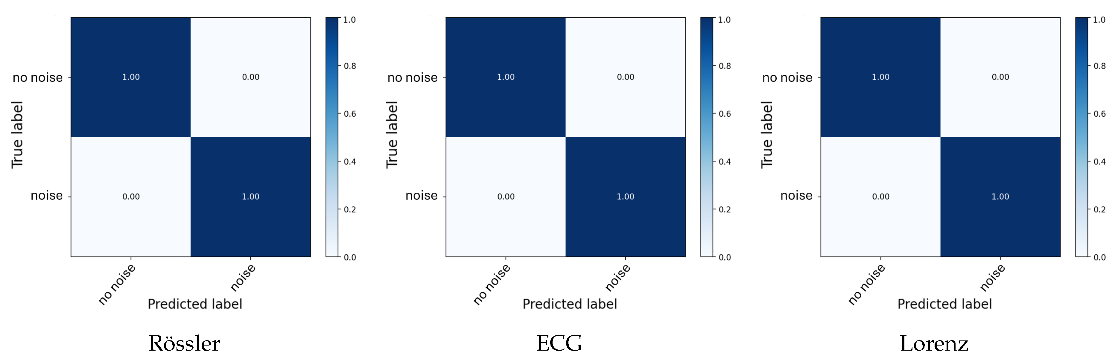
For the initial Noise Category Classification task (Table 2), the models achieved 100% accuracy on the chaotic systems and 99.9% Accuracy for the ECG signal. This provides an average accuracy of 99.9%. As shown in Table 3, the Noise Category + Intensity Classification task achieved perfect performance (100%) for both Lorenz and Rössler. At the same time, the ECG data yielded an F1-score of 88.6% and an accuracy of 89.9%, reflecting the expected reduction in separability due to physiological variability and overlapping noise characteristics. However, the classifier primarily confuses the intensity of the noise, but not between different noise classes, as seen in Figure 4. Across all systems, the average classification accuracy of noise intensities is therefore around 96.2%. Finally, in the binary Noise vs. No-Noise Classification task (Table 4), all systems demonstrate perfect discrimination ability, highlighting that the chosen complexity metrics robustly capture signal contamination across both synthetic and physiological domains.
To visualize model performance across systems, Figure 3, Figure 4 and Figure 5 display the averaged confusion matrices for the Lorenz, Rössler, and ECG experiments. Similar to the tables before, for both chaotic systems (Lorenz and Rössler), the classifiers achieved perfect separation across all noise configurations and intensity levels. All confusion matrices exhibit strong diagonal dominance, indicating complete consistency between predicted and true labels across folds.
In contrast, the ECG-based models exhibited slightly reduced performance for the Noise Category + Intensity Classification task (Figure 4), although the overall detection of noise presence and type remained nearly perfect. Minor misclassifications occurred exclusively between intensity levels of the same noise type rather than between noise categories. For instance, the classifier occasionally confused adjacent low-frequency noise intensities (e.g., between 0.2, 1, and 2), as reflected by the faint off-diagonal entries in the ECG confusion matrix, as seen in Figure 4. These errors primarily represent amplitude-scaling ambiguities rather than conceptual misclassification. Gaussian, pink, and low-frequency noise remained clearly separable.
Figure 3.
Average confusion matrices for all Noise Category classification tasks. Each panel shows normalized confusion results averaged across five folds.
Figure 3.
Average confusion matrices for all Noise Category classification tasks. Each panel shows normalized confusion results averaged across five folds.
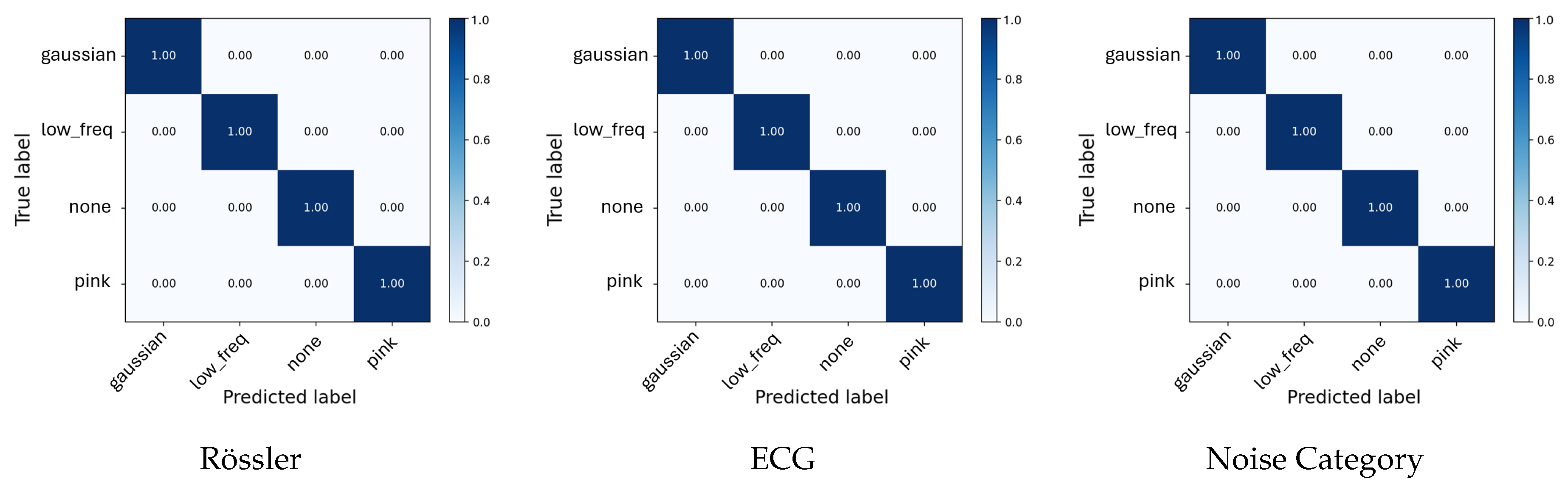
Figure 4.
Average confusion matrices for all Noise Category + Intensity classification tasks. Each panel shows normalized confusion results averaged across five cross-validation folds, highlighting discriminability between noise configurations.
Figure 4.
Average confusion matrices for all Noise Category + Intensity classification tasks. Each panel shows normalized confusion results averaged across five cross-validation folds, highlighting discriminability between noise configurations.
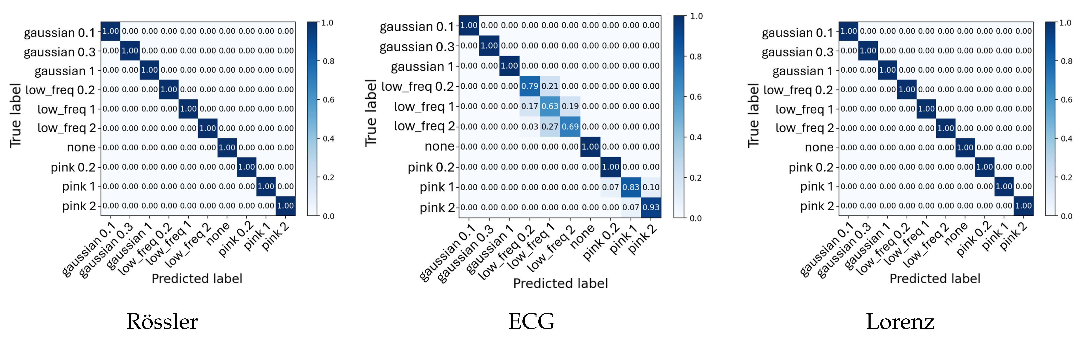
Figure 5.
Average confusion matrices for all Noise Present vs. Not classification tasks. Each panel shows the mean normalized confusion matrix across five folds, illustrating separability between noise types, intensities, and clean signals.
Figure 5.
Average confusion matrices for all Noise Present vs. Not classification tasks. Each panel shows the mean normalized confusion matrix across five folds, illustrating separability between noise types, intensities, and clean signals.
3.2. Feature Importance across Systems
To identify which complexity metrics contributed most to the classification performance, Figure 6, Figure 7 and Figure 8 show the average CatBoost feature importances for all three systems (Lorenz, Rössler, and ECG) grouped by classification task. Each panel displays the top-ranked features and their relative importance averaged across five cross-validation folds.
The relative contribution of each complexity metric to model performance was quantified using CatBoost’s internal feature importance measure, which reflects the mean decrease in impurity across all trees in the ensemble. For each classification task and system, feature importances were averaged over five cross-validation folds, and the corresponding standard deviations were computed to assess stability. Error bars in the plots represent these standard deviations () around the mean importance. In some cases, the lower bounds of these intervals visually extend below zero; this does not indicate negative importance values but merely reflects the uncertainty of the mean estimate when the standard deviation exceeds the mean importance.
In the classification of noise categories (Figure 6), the Condition Number showed the highest importance for the Rössler and Lorenz systems, and ranked third for the ECG data. Entropy-based measures, including Permutation Entropy, Approximate Entropy, and Sample Entropy, were also among the most influential features, particularly for the ECG and Lorenz systems. These metrics provided strong discriminative information for distinguishing between different noise regimes.
For the classification of noise intensity levels (Figure 7), Detrended Fluctuation Analysis (DFA) was an important feature for the Rössler system, while its relevance was limited for the Lorenz and ECG data. Entropy measures again ranked among the top features, with Approximate Entropy and Permutation Entropy showing stable and high importance across systems. The Condition Number remained a key contributor for all datasets, indicating sensitivity to changes in the scale and structure of the signals caused by increasing noise amplitudes.
For the binary detection of noise presence (Figure 8), the models mainly relied on statistical variability metrics such as Standard Deviation, Mean Absolute Deviation, and the Variance of First and Second Derivatives. These measures captured signal fluctuations that effectively separated clean from noisy data. For the ECG signals, Sample Entropy stood out as the most dominant predictor, achieving the highest class-separation contribution among all metrics, suggesting its strong responsiveness to irregularity introduced by noise contamination.
3.3. Metric Sensitivity to Noise Type and Intensity
To analyze how individual complexity measures respond to different noise conditions, boxplots were generated to visualize the distribution of scaled metric values for each noise regime (Gaussian, pink, low-frequency, and no noise). These plots summarize the variability, median, and overall range of each metric across multiple signal realizations, providing an interpretable overview of how noise contamination affects the underlying complexity structure. Broader interquartile ranges or shifted medians indicate higher sensitivity to a specific noise type, while compact or stable distributions suggest robustness against stochastic perturbations.
For the ECG signals, distinct response patterns were observed among the different noise classes as seen in Figure 9 and Figure 10. The dispersion of complexity metric profile for the low frequency noise is less differentiated to the no-noise class compared to the other noises. Clear deviations are seen for statistical attributes (standard deviation, mean absolute deviation), Fisher Information, Coefficient of Variation (CV) and Lempel Ziv Complexity. Pink noise on the other showed a significant increase in entropy based metrics such Approximate, Permutation and Sample Entropy. Condition Number, Standard Deviation and Mean Absolute Deviation showed also increased average values. Fisher Information on the other hand was significantly reduced compared to the no-noise class. The most distinct complexity profile can be found for gaussian noise. Similar to pink noise, all entropy measures exhibited elevated values, indicating higher signal irregularity. Lempel–Ziv complexity, relative singular-value decay, standard deviation, and mean absolute deviation also increased, whereas Fisher Information, SVD Energy, and Condition Number showed consistent decreases. The boxplots of the three noise classes for the Lorenz and Rössler system can be found in the Appendix Figure A3–Figure A6 and Figure A9–Figure A10. A summary comparison between noisy metric regimes and clear signal metric regimes can also be found in the Appendix Figure A11.
To evaluate how increasing noise levels affect the quantitative behavior of complexity measures, line plots were generated for each dynamical system and noise type in Figure 11. Each plot depicts the evolution of mean metric values across three noise intensity levels (low, medium, and high), thereby revealing the sensitivity and scaling characteristics of individual measures in response to increasing stochastic perturbation strength.
For low-frequency noise, the overall behavior appears more stable, as this type of perturbation primarily introduces smooth, slow oscillatory distortions rather than abrupt fluctuations in the time series. Consequently, local dynamical properties and fine-scale variability remain largely preserved. In this regime, condition number and Fisher information (spectral) exhibited the most pronounced increases with higher distortion levels, while the coefficient of variation showed the most notable decrease across noise intensities.
Under pink-noise perturbations, approximate entropy demonstrated the strongest sensitivity to increasing noise amplitude, followed by sample entropy, SVD entropy, and Lempel–Ziv complexity. The Fisher information (spectral) showed a sharp rise between the clean baseline and the lowest perturbation level, but remained comparatively stable thereafter.
In contrast, the Gaussian noise condition yielded the largest overall variation across metrics. Substantial increases with noise intensity were observed for approximate entropy, SVD entropy, sample entropy, and Lempel–Ziv complexity, while significant decreases were found for detrended fluctuation analysis and Fisher information (spectral). The plots for the Lorenz and Rössler system can be found in the Annex Figure A7–Figure A8.
4. Discussion
The present study provides an analysis of various complexity metrics and their potential to characterize and identify noise perturbations in both chaotic and physiological systems. Our findings demonstrate that complexity metrics can serve as robust and interpretable descriptors for detecting, classifying, and quantifying noise using machine learning algorithms. By applying some of these metrics to phase-space trajectories reconstructed from the underlying signals, the study extends traditional time-domain complexity analysis toward a geometrically informed representation that captures higher-order structural distortions caused by noise.
Across all experiments, clear patterns emerged regarding which metrics were most influential for each classification task. For noise intensity classification, the most influential descriptors were Approximate Entropy, Mean Absolute Deviation, and the Condition Number of the embedded attractor. Fisher Information contributed consistently across all three datasets, reflecting its theoretical sensitivity to local gradient structures and information density. Depending on the system, additional metrics such as Detrended Fluctuation Analysis were particularly relevant, especially for the Rössler system, where long-range correlations and slow attractor rotations make scaling-based measures more informative.
For noise category classification, the Condition Number emerged as the most dominant feature, suggesting that geometric anisotropy within the reconstructed attractor space provides a highly discriminative representation of different noise types. Entropy-based measures, especially Approximate Entropy, Sample Entropy, and Permutation Entropy, were also strong predictors, particularly for the ECG and Lorenz systems. These results indicate that while entropy measures effectively capture irregularity and loss of predictability, the structural deformation of the manifold encoded by SVD-derived metrics can reveal complementary aspects of noise-specific degradation.
Interestingly, for the simpler noise presence detection task, Sample Entropy was by far the most informative metric in the ECG system. This observation aligns with its established role in quantifying signal quality and physiological irregularity, as shown in previous biomedical studies such as Holgado-Cuadrado et al. [15]. In contrast, for the chaotic systems, simpler statistical measures such as Standard Deviation, Mean Absolute Deviation, and the Variance of Derivatives (first and second order) were the most decisive indicators of noise injection. This distinction suggests that while entropy-based measures capture fine-grained irregularities in quasi-periodic biological signals, the global statistical variability of chaotic trajectories is already sufficient to identify stochastic contamination.
The observed importance of entropy measures aligns with earlier findings in biomedical and dynamical signal research. Cuesta-Frau et al. [4] demonstrated that Approximate Entropy is highly sensitive to outliers and measurement artefacts in noisy EEG signals, which likely contributes to its discriminative power in detecting subtle perturbations. Likewise, as postulated by Sara Maria et al. Mariani et al. [12], noisy signals generally exhibit lower information content compared to clean signals, a relationship corroborated by our observed negative correlation between Fisher Information and increasing noise intensity in Gaussian and Pink noise (ECG data) in Figure 11. Moreover, Christoph Bandt and Bernd Pompe originally proposed that Permutation Entropy provides an effective complexity measure for chaotic time series, particularly under dynamical and observational noise [21]. Our results partially confirm this claim. While Permutation Entropy indeed responded to stochastic perturbations, other metrics, such as the Condition Number and Approximate Entropy, showed greater descriptive and predictive capacity for noise classification in our controlled experiments. Our observation of increased permutation entropy in all three noise categories also aligns with the findings of Ricci and Politi [11], who reported an increase of Permutation Entropy under weak noise.
Makowski et al. [10] investigated a set of twelve complexity metrics implemented in NeuroKit2 and analyzed their mean responses to varying colored-noise intensities. While their results provided a valuable benchmark for sensitivity comparison, the study focused exclusively on descriptive averages without predictive modeling. Consequently, the observed behaviors of individual metrics were difficult to interpret in relation to one another. In our experiments, SVD Entropy, which Makowski et al. identified as strongly noise-responsive, showed a comparable pattern. It exhibited strong positive increases with noise intensity in the ECG and Rössler system, but some negative trends in the Lorenz system for Pink and Low Frequency noise. However, Sample Entropy displayed positive trends with Gaussian noise intensity in the Lorenz system. This divergence highlights that the relationship between individual complexity metrics and noise intensity cannot be universally generalized. It is defined by the intrinsic geometry, potential autocorrelation, and timescale of the underlying system.
A related study by Holgado-Cuadrado et al. [15] analyzed the potential of machine learning models combined with a limited set of time- and frequency-domain features, including Sample Entropy, to classify ECG segments according to clinical noise severity. Unlike our framework, which differentiates both noise type and intensity, Holgado et al. treated all noise sources identically and categorized signals into five quality levels ranging from “clean” to “high noise.” Their model achieved a precision of 78% and recall of 80%, demonstrating the viability of ML-based noise quality assessment in real-world ECG recordings. Our findings extend their work by showing that a broader set of complexity metrics substantially improves discriminative power, particularly in differentiating not only the nature but also the degree of noise perturbations. Furthermore, by using synthetic signals with controlled perturbations, our framework provides interpretable ground-truth relationships between specific metrics and noise characteristics. This allows future studies to apply these metrics to real clinical ECG or EEG data to investigate whether the same noise sensitivity patterns persist under uncontrolled conditions.
In contrast to studies focusing solely on physiological signals, Kumar and Sharma [14] employed classical statistical features (such as kurtosis, zero-crossing rate, and dynamic range) to detect and classify different noise regimes in ECG data. Their method achieved a high accuracy of 97.19% for distinguishing four primary noise types and their combinations. Our approach advances this line of research by extending the feature space to include higher-order complexity measures and by systematically controlling noise intensity levels. This not only allowed for a direct comparison of feature sensitivities but also enabled us to achieve almost 100% noise detection and category classification accuracy across all three datasets. The results demonstrate that complexity-based descriptors can capture the nonlinear and multifaceted effects of noise with greater expressiveness than purely statistical indicators.
While the feature importance analysis provides valuable insights into which complexity metrics most strongly contributed to model performance, these results should be interpreted with caution. The relative importance values derived from tree-based models such as CatBoost are inherently dependent on the model’s internal structure, data partitioning, and random initialization. Consequently, small variations in the training process or noise composition can alter the resulting feature hierarchy. High feature importance does not necessarily imply that other metrics are uninformative. It indicates that a given feature was sufficient to achieve class separation under the specific decision-tree configuration. For instance, the dominance of Sample Entropy in distinguishing noisy from clean ECG signals reflects its discriminative efficiency within the trained model, not the absence of complementary information in related metrics. A more comprehensive explainability analysis combining multiple Explainable AI approaches, such as permutation importance, Shapley additive explanations interaction values, and partial dependence analyses, will be necessary in future work to fully characterize the interdependencies among complexity measures and their respective roles in noise classification.
In general, future research is necessary to validate the observed feature sensitivities on empirical datasets, such as long-term clinical ECG recordings or real-world sensor signals with mixed and non-stationary noise profiles. Second, the approach could be expanded from discrete classification toward continuous noise estimation or regression modelling, enabling quantitative tracking of noise levels over time. From a theoretical perspective, future studies may explore how distinct noise regimes alter phase-space geometry and information flow within the attractor, linking complexity-based measures more directly to dynamical invariants such as Lyapunov spectra or correlation dimension.
5. Conclusions
This study systematically investigated which complexity metrics most effectively characterize stochastic perturbations in time series data, using two chaotic systems (Rössler and Lorenz) and one physiological signal (ECG). The results demonstrate that employing complexity metrics as the sole feature set enables highly accurate prediction of noise presence, noise type, and noise intensity across all systems. Average classification accuracies reached 99.9% for both noise detection and noise-type identification, and 96.2% for noise-intensity classification, underscoring the strong discriminative power of the selected metrics. By analyzing the feature sensitivity and importance across systems and noise regimes, the study revealed that the descriptive influence of each metric varies substantially depending on the dynamical properties of the underlying signal and the specific prediction objective. Approximate Entropy, Mean Absolute Deviation, and Condition Number exhibited high relevance for noise-intensity classification, while Condition Number, Sample Entropy, and Permutation Entropy contributed most strongly to differentiating noise categories. For the binary detection of noise presence, simpler statistical descriptors such as Standard Deviation, Mean Absolute Deviation, and Variance of Derivatives dominated, whereas Sample Entropy proved particularly sensitive for detecting noise in ECG signals. In general, Entropy values, Spectral Fisher Information, and Condition Number showed high discriminative power for the ECG signal analysis and noise differentiation. In the Lorenz system, Fisher Information, Condition Number, Variance of the First Derivative, and Approximate Entropy demonstrated distinct complexity profiles for individual noise categories, showing strong relevance across different noise classification tasks. For the Rössler system, Detrended Fluctuation Analysis, Condition Number, and statistical descriptors such as the Variance of the Second Derivative, Standard Deviation, and Mean Absolute Deviation displayed characteristic patterns that enabled clear differentiation between noise regimes. The analysis also showed that across all noise regimes, Approximate, Sample, and SVD Entropy are most sensitive to weak and strong noise pollution. Overall, the findings confirm that complexity-based measures capture the essential structural and statistical signatures of stochastic contamination in both chaotic and physiological time series. It was also shown that the phase-space embedded computation of complexity metrics (e.,g Spectral Fisher Information, Condition Number) is an important factor for noise classification. Future research should focus on validating these results using empirical datasets, such as long-term ECG and EEG recordings, and extending the framework toward continuous noise-level estimation.
Author Contributions
Conceptualization, Kevin Mallinger and Sebastian Raubitzek; methodology, Kevin Mallinger; software, Kevin Mallinger; validation, Kevin Mallinger and Sebastian Raubitzek; formal analysis, Kevin Mallinger; investigation, Kevin Mallinger; resources, Kevin Mallinger; data curation, Kevin Mallinger; writing—original draft preparation, Kevin Mallinger, Sebastian Raubitzek; writing—review and editing, Kevin Mallinger and Sebastian Raubitzek; visualization, Kevin Mallinger; supervision, Kevin Mallinger; project administration, Kevin Mallinger; funding acquisition, Sebastian Schrittwieser, Edgar Weippl. All authors have read and agreed to the published version of the manuscript.
Funding
SBA Research (SBA-K1) is a COMET Centre within the COMET – Competence Centers for Excellent Technologies Programme and funded by BMK, BMAW, and the federal state of Vienna. COMET is managed by FFG. Additionally, the financial support by the Austrian Federal Ministry of Labour and Economy, the National Foundation for Research, Technology and Development and the Christian Doppler Research Association is gratefully acknowledged.
Data Availability Statement
All data is publicly reproducible following the instruction given in the section "Data Sources and Signal Generation". A ready-to-use implementation of the experiment and noise classification pipeline is available in a corresponding GitHub repository [github.com/CORE-Research-Group/Noise-Prediction-Complexity]
Conflicts of Interest
The funders had no role in the design of the study; in the collection, analyses, or interpretation of data; in the writing of the manuscript; or in the decision to publish the results.
Abbreviations
The following abbreviations are used in this manuscript:
| ML | Machine Learning |
| SVD | Singular Value Decomposition |
| ECG | Electrocardiogram |
| EEG | Electroencephalogram |
| DFA | Detrended Fluctuation Analysis |
| CV | Coefficient of Variation |
| MAD | Mean Absolute Deviation |
| SD | Standard Deviation |
Appendix A. Clean and Distorted Systems Used in the Study
Figure A1.
Combined visualization of Lorenz system signals under medium noise intensity across noise types.
Figure A1.
Combined visualization of Lorenz system signals under medium noise intensity across noise types.
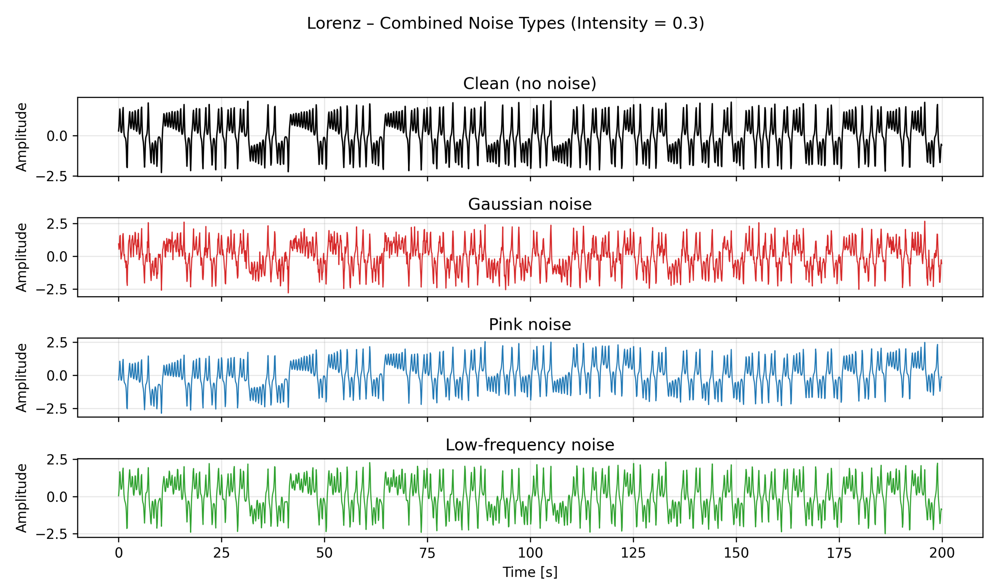
Figure A2.
Combined visualization of ECG signals under medium noise intensity across noise types.
Appendix B. Additional Visualizations of Complexity Metric Sensibility
Figure A3.
Boxplots of complexity metrics for the Rössler system under Gaussian and pink noise regimes.
Figure A3.
Boxplots of complexity metrics for the Rössler system under Gaussian and pink noise regimes.
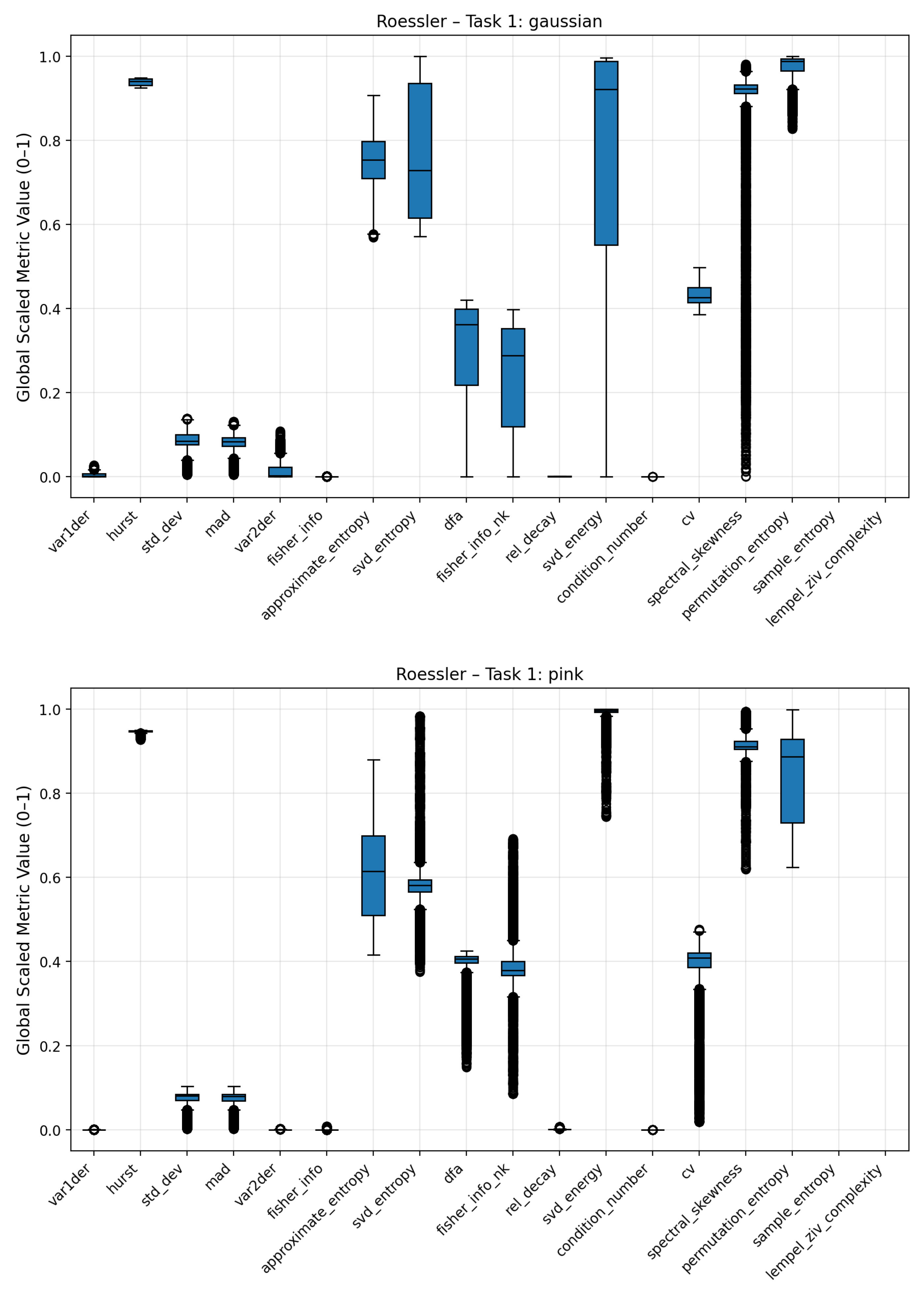
Figure A4.
Boxplots of complexity metrics for the Rössler system under low-frequency noise and no-noise regimes.
Figure A4.
Boxplots of complexity metrics for the Rössler system under low-frequency noise and no-noise regimes.
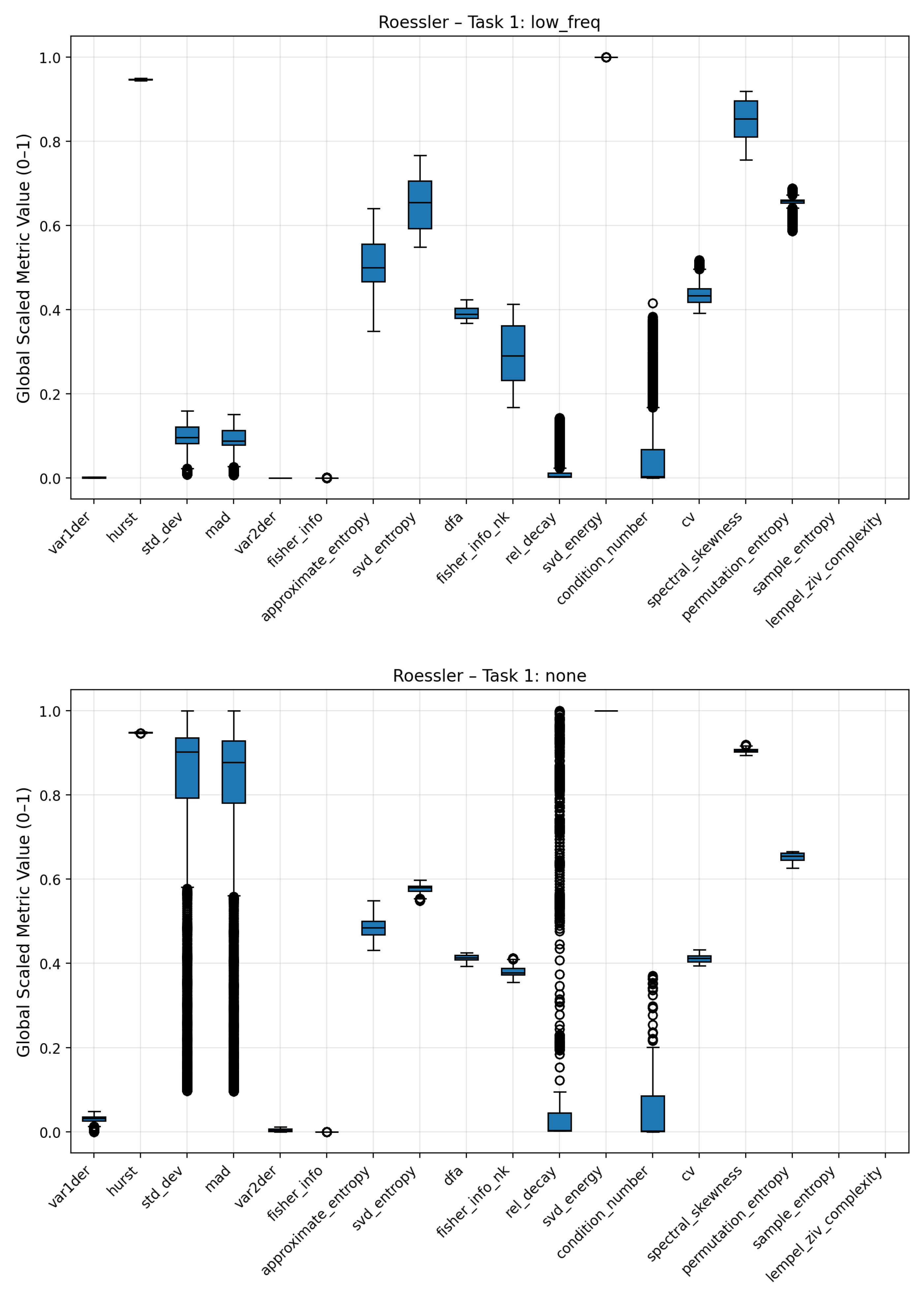
Figure A5.
Boxplots of complexity metrics for the Lorenz system under Gaussian and pink noise regimes.
Figure A5.
Boxplots of complexity metrics for the Lorenz system under Gaussian and pink noise regimes.
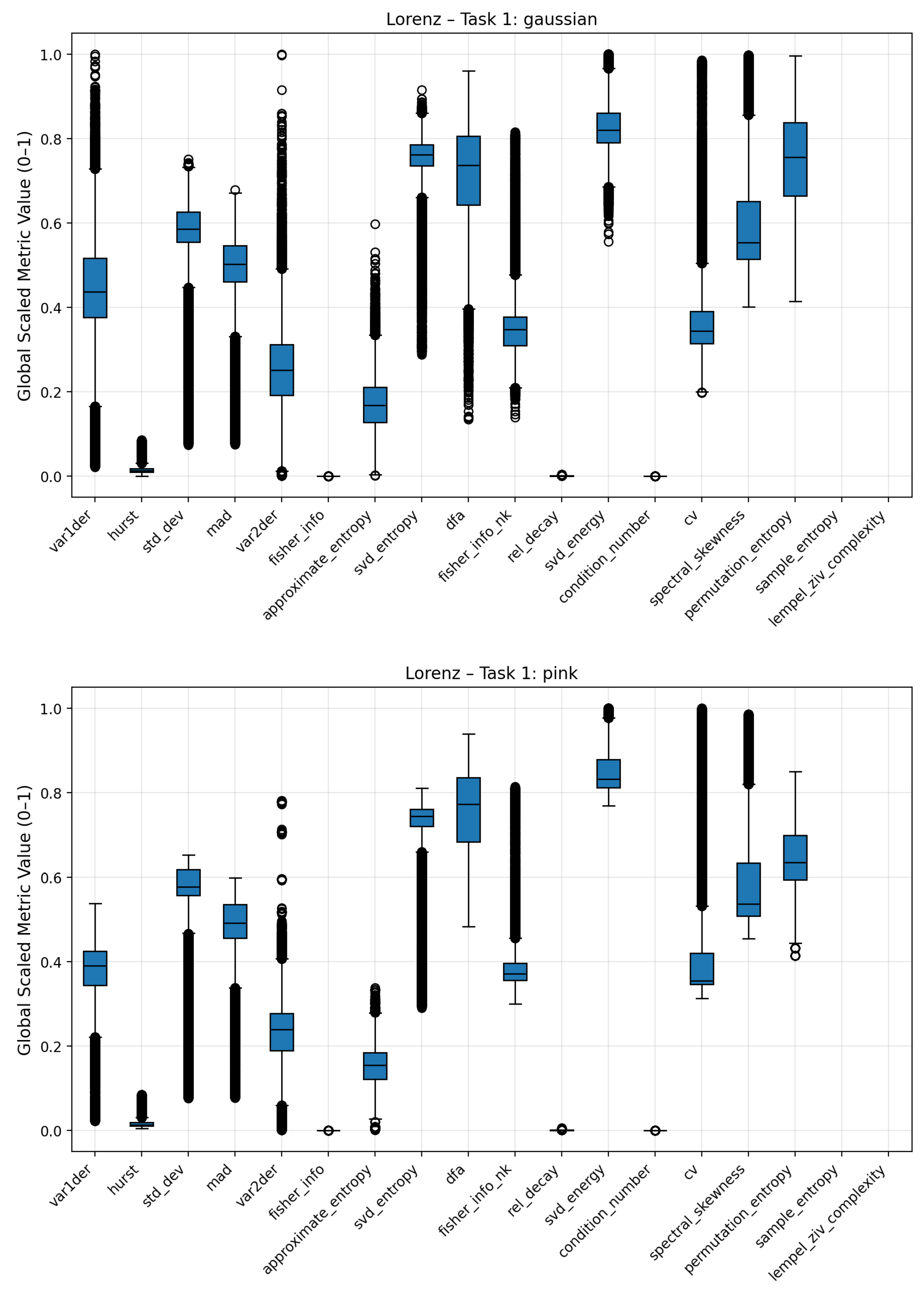
Figure A6.
Boxplots of complexity metrics for the Lorenz system under low-frequency noise and the clean baseline (no noise).
Figure A6.
Boxplots of complexity metrics for the Lorenz system under low-frequency noise and the clean baseline (no noise).
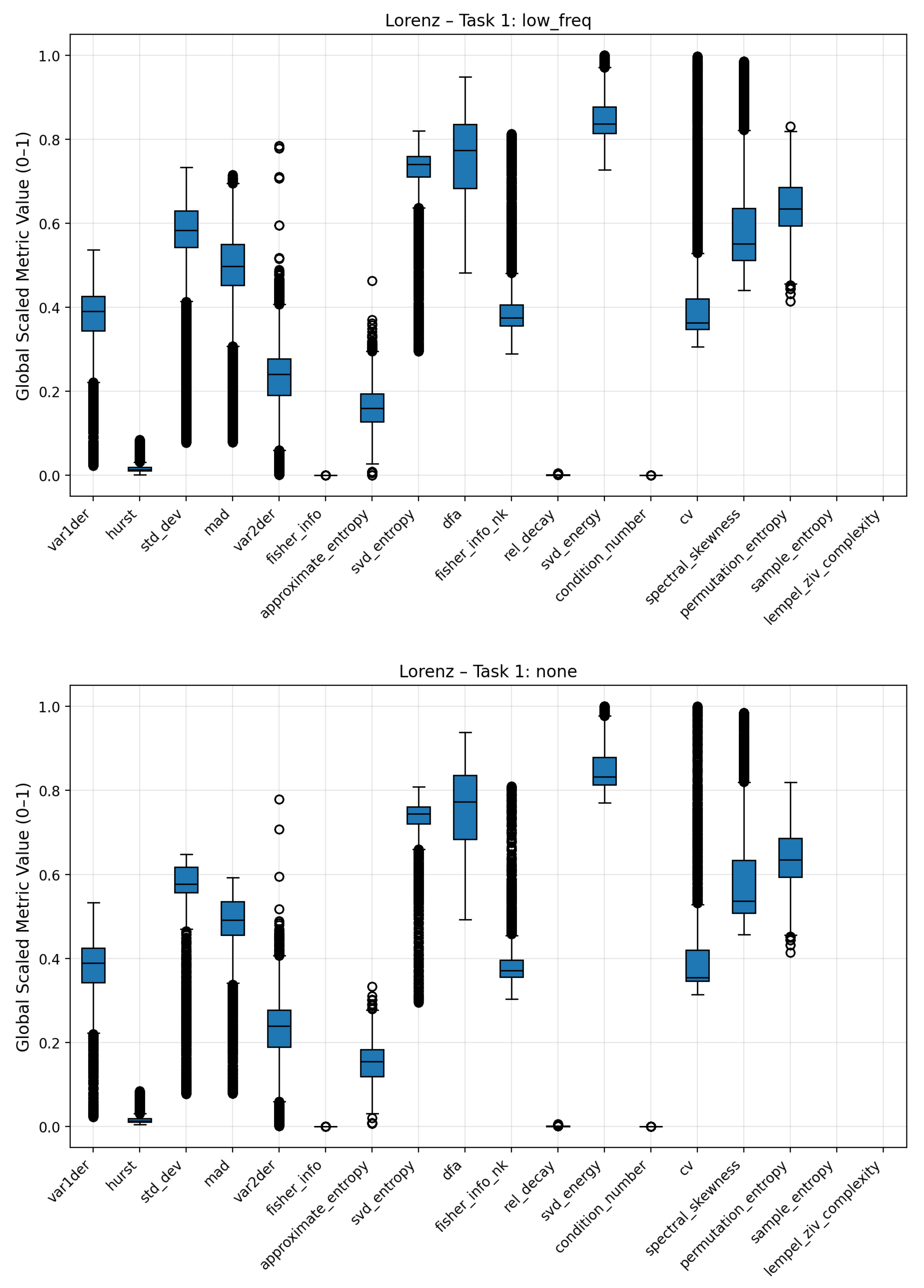
Figure A7.
Average trajectories of complexity metrics for the Rössler system across increasing noise intensities. Each line represents a specific complexity measure, showing how its mean value evolves under Gaussian, pink, and low-frequency noise. Metrics exhibiting smooth or monotonic trends indicate systematic sensitivity to noise strength.
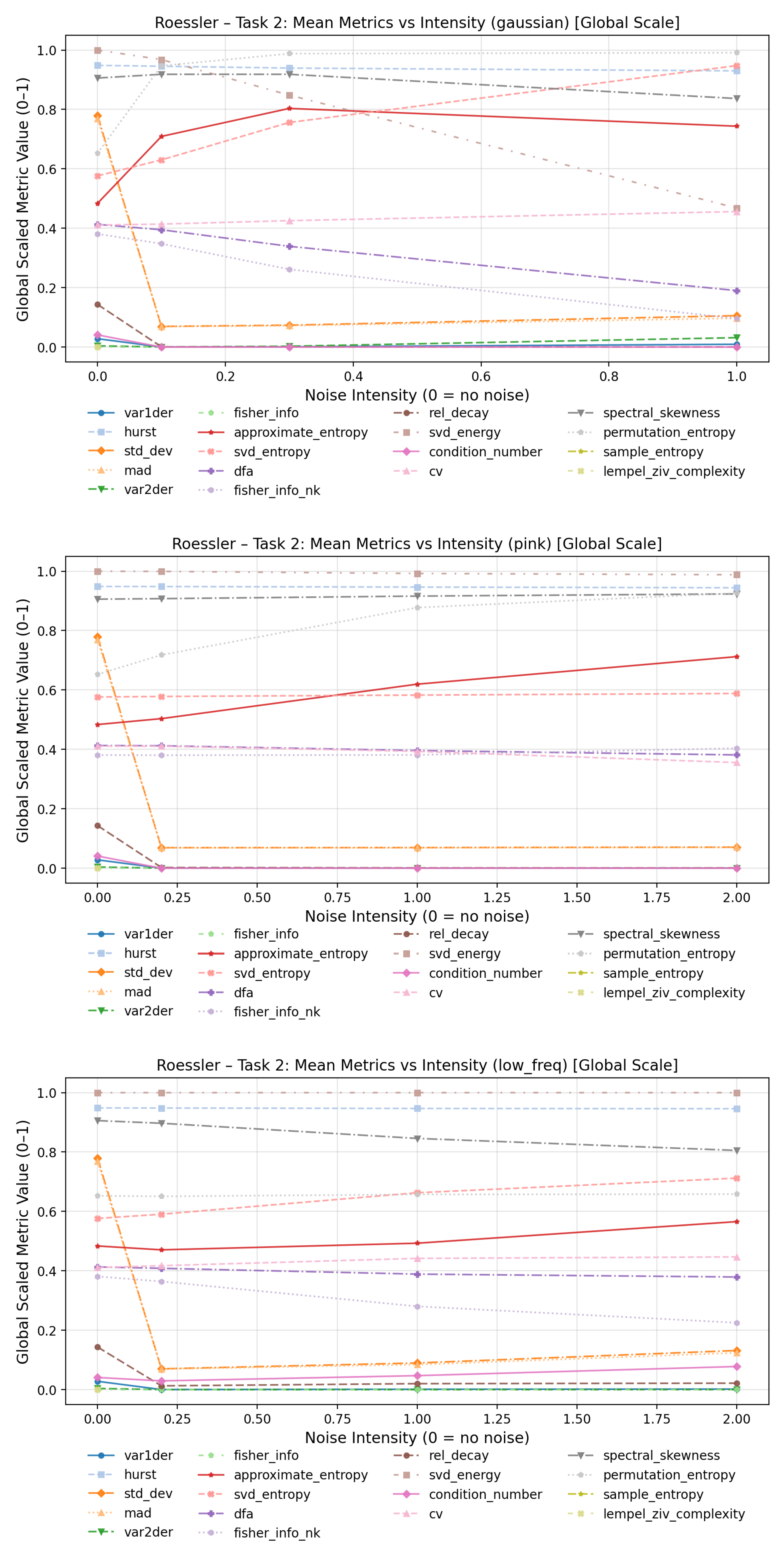
Figure A8.
Average trajectories of complexity metrics for the Lorenz system under Gaussian, pink, and low-frequency noise across increasing intensities. The observed metric evolution patterns reveal both system-specific and metric-specific scaling responses to stochastic distortion.
Figure A8.
Average trajectories of complexity metrics for the Lorenz system under Gaussian, pink, and low-frequency noise across increasing intensities. The observed metric evolution patterns reveal both system-specific and metric-specific scaling responses to stochastic distortion.
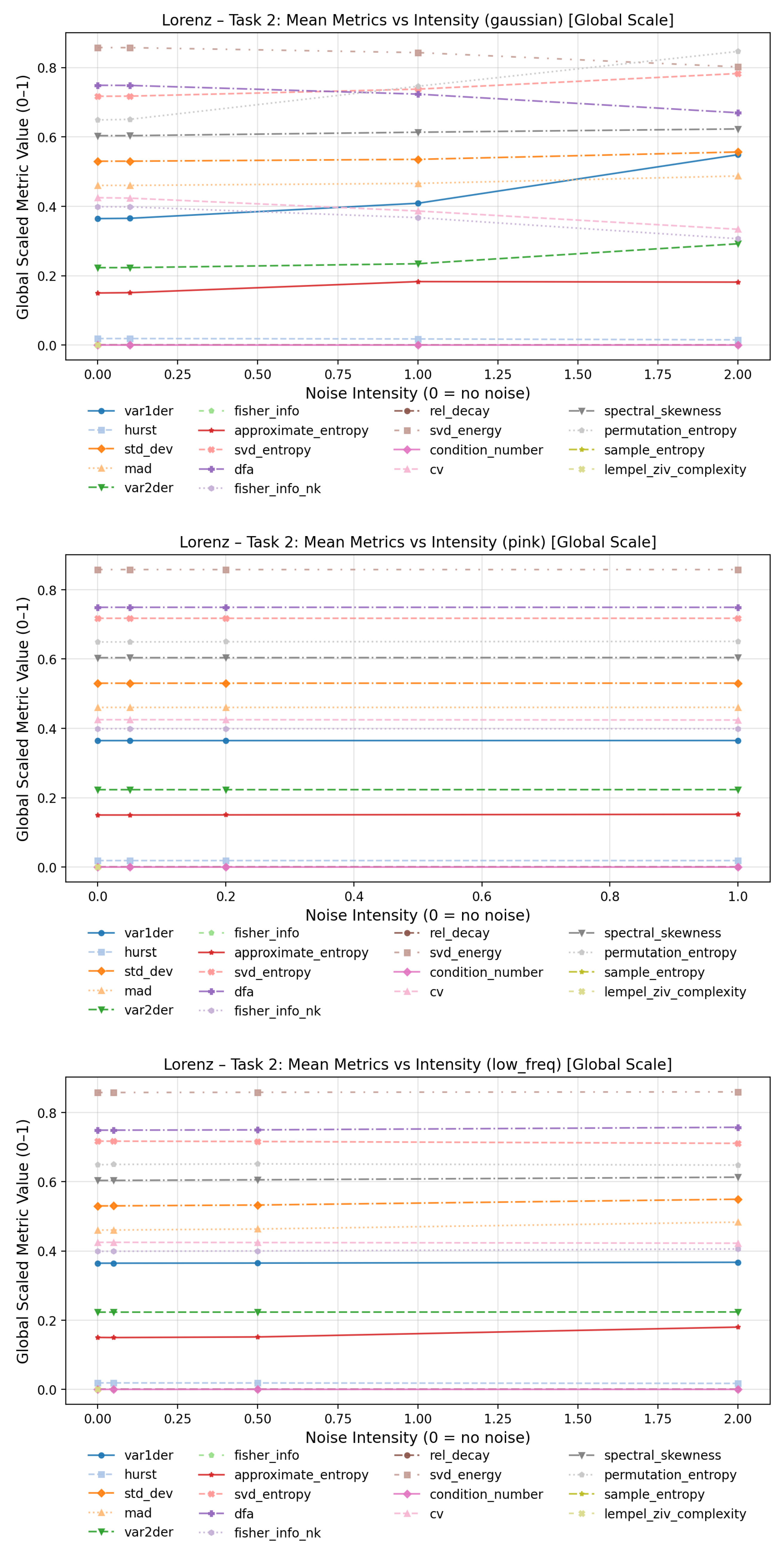
Figure A9.
Boxplots of Rössler system complexity metrics under clean (top) and noisy (bottom) conditions. The separation between distributions illustrates how stochastic perturbations globally influence the variability and median values of the metrics.
Figure A9.
Boxplots of Rössler system complexity metrics under clean (top) and noisy (bottom) conditions. The separation between distributions illustrates how stochastic perturbations globally influence the variability and median values of the metrics.
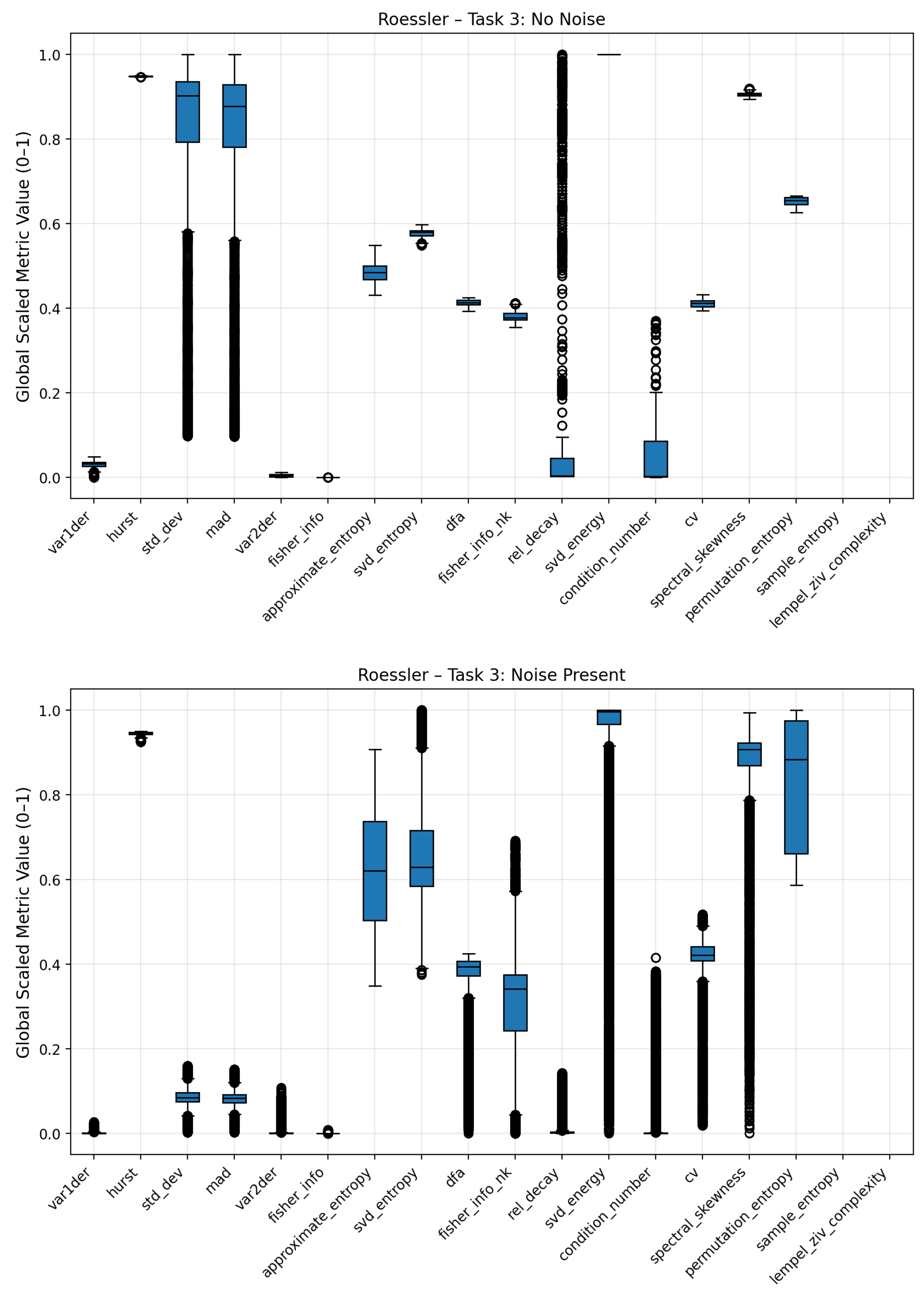
Figure A10.
Boxplots of Lorenz system complexity metrics comparing clean and noisy conditions. The results emphasize consistent shifts across several metrics, confirming the framework’s ability to detect general noise presence in chaotic dynamics.
Figure A10.
Boxplots of Lorenz system complexity metrics comparing clean and noisy conditions. The results emphasize consistent shifts across several metrics, confirming the framework’s ability to detect general noise presence in chaotic dynamics.
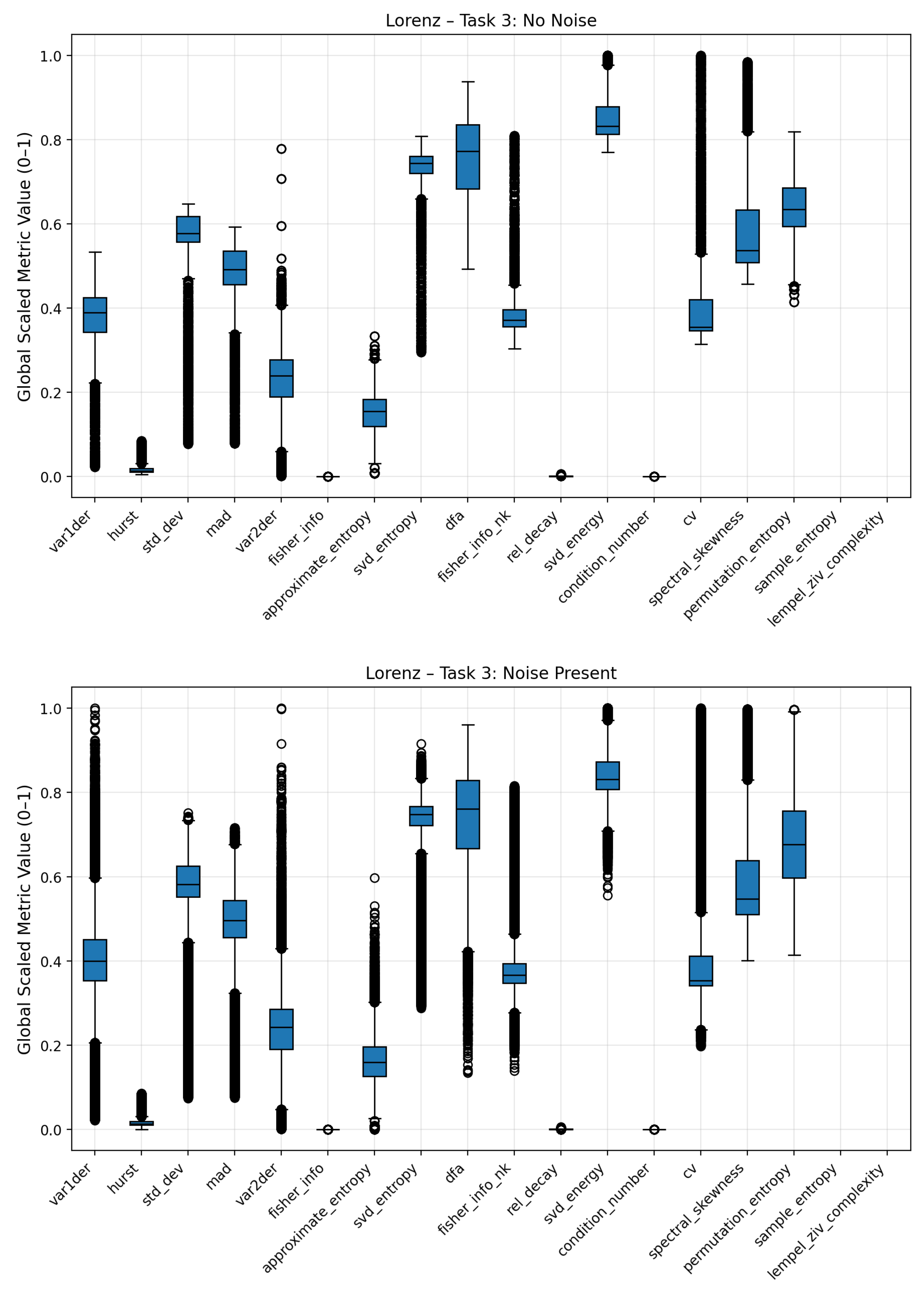
Figure A11.
Boxplots of ECG complexity metrics for clean (top) and noisy (bottom) conditions.

References
- Hutton, C.; Josephs, O.; Stadler, J.; Featherstone, E.; Reid, A.; Speck, O.; Bernarding, J.; Weiskopf, N. The Impact of Physiological Noise Correction on fMRI at 7 T. NeuroImage 2011, 57, 101–112. [Google Scholar] [CrossRef] [PubMed]
- Vincent, P.; Larochelle, H.; Bengio, Y.; Manzagol, P.-A. Extracting and Composing Robust Features with Denoising Autoencoders. In Proceedings of the 25th International Conference on Machine Learning (ICML ’08); Association for Computing Machinery: New York, NY, USA, 2008; pp. 1096–1103. [Google Scholar] [CrossRef]
- Jia, Y.; Pei, H.; Liang, J.; Zhou, Y.; Yang, Y.; Cui, Y.; Xiang, M. Preprocessing and Denoising Techniques for Electrocardiography and Magnetocardiography: A Review. Bioengineering 2024, 11, 1109. [Google Scholar] [CrossRef] [PubMed]
- Cuesta-Frau, D.; Miró-Martínez, P.; Jordán Núñez, J.; Oltra-Crespo, S.; Molina Picó, A. Noisy EEG signals classification based on entropy metrics. Performance assessment using first and second generation statistics. Comput. Biol. Med. 2017, 87, 141–151. [Google Scholar] [CrossRef] [PubMed]
- Schrittwieser, S.; Wimmer, E.; Mallinger, K.; Kochberger, P.; Lawitschka, C.; Raubitzek, S.; Weippl, E. R. Modeling obfuscation stealth through code complexity. In European Symposium on Research in Computer Security; Springer: Cham, 2023; pp. 392–408. [Google Scholar]
- Mallinger, K.; Raubitzek, S.; Neubauer, T.; Lade, S. Potentials and limitations of complexity research for environmental sciences and modern farming applications. Curr. Opin. Environ. Sustain. 2024, 67, 101429. [Google Scholar] [CrossRef]
- König, P.; Raubitzek, S.; Schatten, A.; Toth, D.; Obermann, F.; König, C.; Mallinger, K. Boost-Classifier-Driven Fault Prediction Across Heterogeneous Open-Source Repositories. Big Data Cogn. Comput. 2025, 9. [Google Scholar] [CrossRef]
- S. Raubitzek and T. Neubauer, “Taming the Chaos in Neural Network Time Series Predictions,” Entropy, vol. 23, no. 11, p. 1424, 2021. [CrossRef]
- S. Raubitzek and T. Neubauer, “Combining Measures of Signal Complexity and Machine Learning for Time Series Analysis: A Review,” Entropy, vol. 23, no. 12, p. 1672, 2021. [CrossRef]
- Makowski, D.; Te, A.S.; Pham, T.; Lau, Z.J.; Chen, S.H.A. The Structure of Chaos: An empirical comparison of fractal physiology complexity indices using NeuroKit2. Entropy 2022, 24, 1036. [Google Scholar] [CrossRef] [PubMed]
- Ricci, L.; Politi, A. Permutation Entropy of Weakly Noise-Affected Signals. Entropy 2022, 24. [Google Scholar] [CrossRef] [PubMed]
- Mariani, S.; Borges, A.F.; Henriques, T.; Goldberger, A.L.; Costa, M.D. Use of multiscale entropy to facilitate artifact detection in electroencephalographic signals. In Proc. Annu. Int. Conf. IEEE Eng. Med. Biol. Soc.; IEEE: Milan, Italy, 2015; pp. 7869–7872. [Google Scholar] [CrossRef]
- Hayn, D.; Jammerbund, B.; Schreier, G. ECG quality assessment for patient empowerment in mHealth applications. In Computing in Cardiology; IEEE: Hangzhou, China, 2011; pp. 353–356. [Google Scholar] [CrossRef]
- Kumar, P.; Sharma, V.K. Detection and classification of ECG noises using decomposition on mixed codebook for quality analysis. Healthc. Technol. Lett. 2020, 7, 18–24. [Google Scholar] [CrossRef] [PubMed]
- Holgado-Cuadrado, R.; Plaza-Seco, C.; Lovisolo, L.; Blanco-Velasco, M. Characterization of noise in long-term ECG monitoring with machine learning based on clinical criteria. Med. Biol. Eng. Comput. 2023, 61, 2227–2240. [Google Scholar] [CrossRef] [PubMed]
- Monteiro, T.; da Silva, L.; Cardoso, C.; Reis, C.; Almeida, P. Assessing electrocardiogram quality: A deep learning framework for noise detection and classification. Biomed. Signal Process. Control 2025, 90, 105961. [Google Scholar] [CrossRef]
- Boaretto, B.R.R.; Budzinski, R.C.; Rossi, K.L.; Prado, T.L.; Lopes, S.R.; Masoller, C. Discriminating chaotic and stochastic time series using permutation entropy and artificial neural networks. Sci. Rep. 2021, 11, 15789. [Google Scholar] [CrossRef] [PubMed]
- Takens, F. Detecting strange attractors in turbulence. In Dynamical Systems and Turbulence, Warwick 1980; Rand, D.A., Young, L.S., Eds.; Lecture Notes in Mathematics; Springer: Berlin, Germany, 1981; Volume 898, pp. 366–381. [Google Scholar] [CrossRef]
- Pincus, S. M. Approximate entropy as a measure of system complexity. Proc. Natl. Acad. Sci. U.S.A. 1991, 88, 2297–2301. [Google Scholar] [CrossRef] [PubMed]
- Richman, J.S.; Moorman, J.R. Physiological time-series analysis using approximate entropy and sample entropy. Am. J. Physiol. Heart Circ. Physiol. 2000, 278, H2039–H2049. [Google Scholar] [CrossRef] [PubMed]
- Bandt, C.; Pompe, B. Permutation entropy: A natural complexity measure for time series. Phys. Rev. Lett. 2002, 88, 174102. [Google Scholar] [CrossRef] [PubMed]
- Roberts, S. J.; Penny, W.; Rezek, I. Temporal and spatial complexity measures for electroencephalogram-based brain–computer interfacing. Med. Biol. Eng. Comput. 1999, 37, 93–98. [Google Scholar] [CrossRef] [PubMed]
- Peng, C.-K.; Buldyrev, S. V.; Havlin, S.; Simons, M.; Stanley, H. E.; Goldberger, A. L. Mosaic organization of DNA nucleotides. Phys. Rev. E 1994, 49, 1685–1689. [Google Scholar] [CrossRef] [PubMed]
- Hurst, H. E. Long-term storage capacity of reservoirs. Trans. Am. Soc. Civil Eng. 1951, 116, 770–799. [Google Scholar] [CrossRef]
- Wolf, A.; Swift, J.B.; Swinney, H.L.; Vastano, J.A. Determining Lyapunov exponents from a time series. Physica D 1985, 16, 285–317. [Google Scholar] [CrossRef]
- Fisher, R. A. On the mathematical foundations of theoretical statistics. Philos. Trans. R. Soc. London Ser. A 1922, 222, 309–368. [Google Scholar]
- S. Raubitzek, T. Neubauer, J. Friedrich, and A. Rauber, “Interpolating Strange Attractors via Fractional Brownian Bridges,” Entropy, vol. 24, no. 5, p. 718, 2022. [CrossRef]
- A. C. Antoulas, D. C. Sorensen, and Y. Zhou, “On the decay rate of Hankel singular values and related issues,” Systems & Control Letters, vol. 46, no. 5, pp. 323–342, 2002. [CrossRef]
- H. B. Razafindradina, P. A. Randriamitantsoa, and N. R. Razafindrakoto, “Image Compression with SVD: A New Quality Metric Based on Energy Ratio,” CoRR, vol. abs/1701.06183, 2017. Available: http://arxiv.org/abs/1701.06183.
- A. Edelman, “Eigenvalues and Condition Numbers of Random Matrices,” SIAM Journal on Matrix Analysis and Applications, vol. 9, no. 4, pp. 543–560, 1988. [CrossRef]
- D. N. Joanes and C. A. Gill, “Comparing Measures of Sample Skewness and Kurtosis,” Journal of the Royal Statistical Society: Series D (The Statistician), vol. 47, no. 1, pp. 183–189, 1998. [CrossRef]
- S. Raubitzek and T. Neubauer, “Reconstructed Phase Spaces and LSTM Neural Network Ensemble Predictions,” Engineering Proceedings, vol. 18, no. 1, p. 40, 2022. [CrossRef]
- A. Quarteroni, R. Sacco, and F. Saleri. Numerical Mathematics. Springer Berlin, Heidelberg, 2nd edition, vol. 37, 2007. [CrossRef]
Figure 1.
Classification pipeline used in the study. Clean signals from chaotic and physiological systems are perturbed with Gaussian, pink, and low–frequency noise at varying intensities. Complexity-based features are extracted from the resulting time series and fed into supervised models for identifying noise presence, type, and intensity. Finally we analyze which features are the most important ones in the different classification tasks.
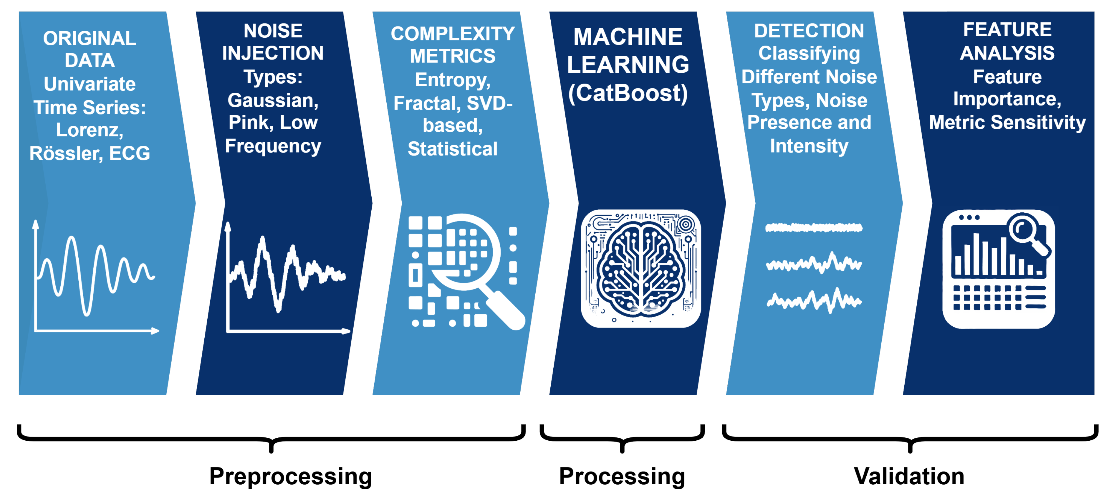
Figure 2.
Combined visualization of the Rössler system’s x-component for the clean case and under medium-intensity Gaussian, pink, and low-frequency noise.
Figure 2.
Combined visualization of the Rössler system’s x-component for the clean case and under medium-intensity Gaussian, pink, and low-frequency noise.
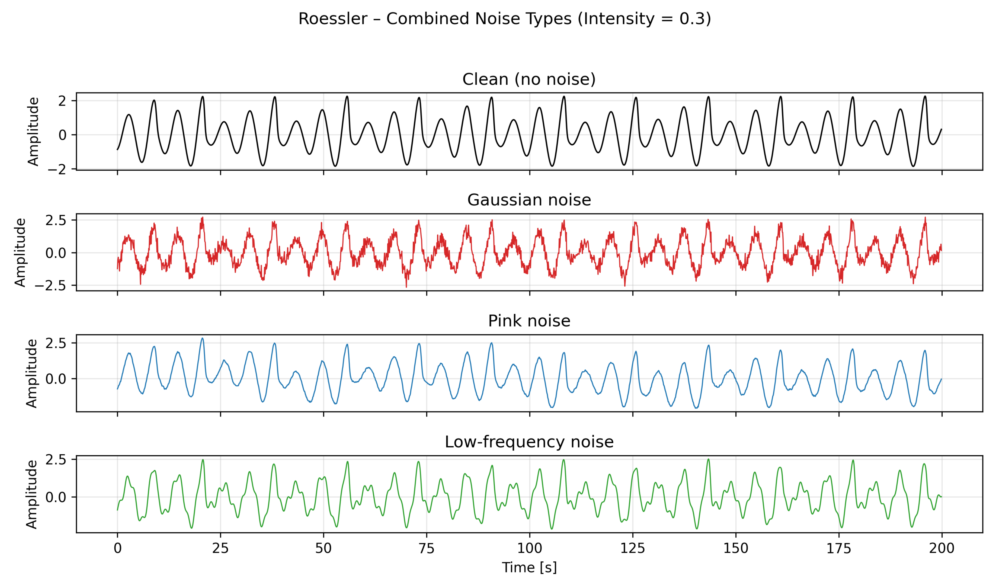
Figure 6.
Average feature importance for the Noise Category Classification task across all systems. Each bar chart represents the mean normalized importance values obtained from CatBoost models.
Figure 6.
Average feature importance for the Noise Category Classification task across all systems. Each bar chart represents the mean normalized importance values obtained from CatBoost models.

Figure 7.
Average feature importance for the Noise Category + Intensity Classification task. The bar charts highlight which complexity metrics scale most systematically with increasing noise levels.
Figure 7.
Average feature importance for the Noise Category + Intensity Classification task. The bar charts highlight which complexity metrics scale most systematically with increasing noise levels.
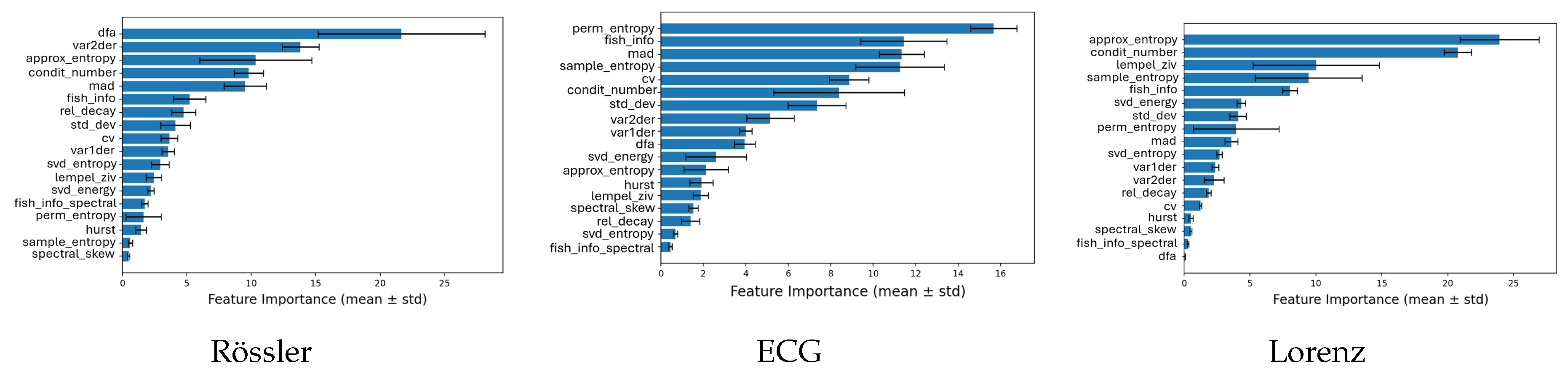
Figure 8.
Average feature importance for the Noise Present vs. Not Classification task across systems. These results illustrate the sensitivity of each metric to the presence of noise, independent of its type or intensity.
Figure 8.
Average feature importance for the Noise Present vs. Not Classification task across systems. These results illustrate the sensitivity of each metric to the presence of noise, independent of its type or intensity.
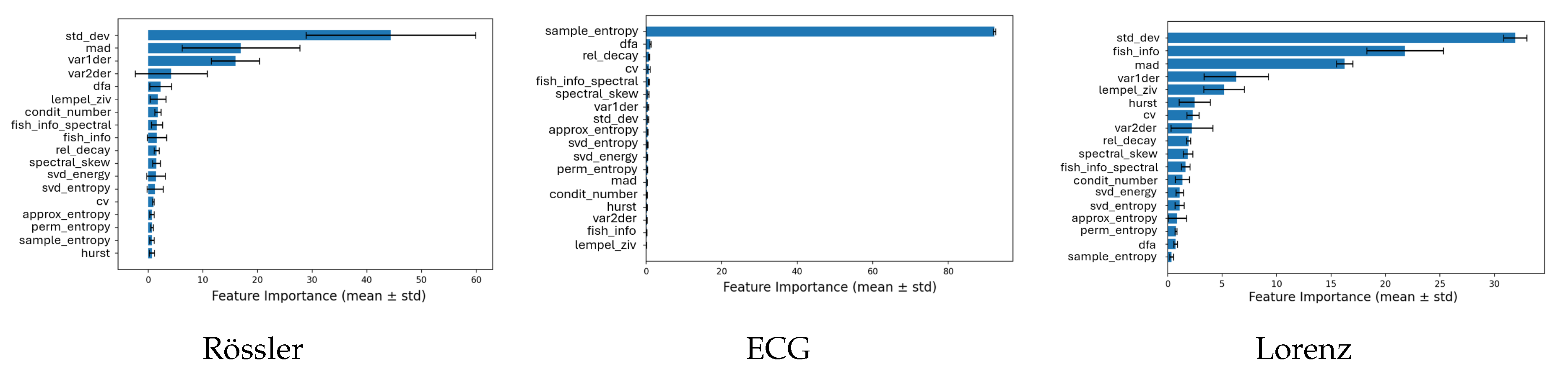
Figure 9.
Boxplots of complexity metrics for the ECG signal under Gaussian and pink noise. Both panels highlight how stochastic perturbations influence entropy- and variance-based descriptors. All metric values are scaled to the 0–1 range for comparability.
Figure 9.
Boxplots of complexity metrics for the ECG signal under Gaussian and pink noise. Both panels highlight how stochastic perturbations influence entropy- and variance-based descriptors. All metric values are scaled to the 0–1 range for comparability.
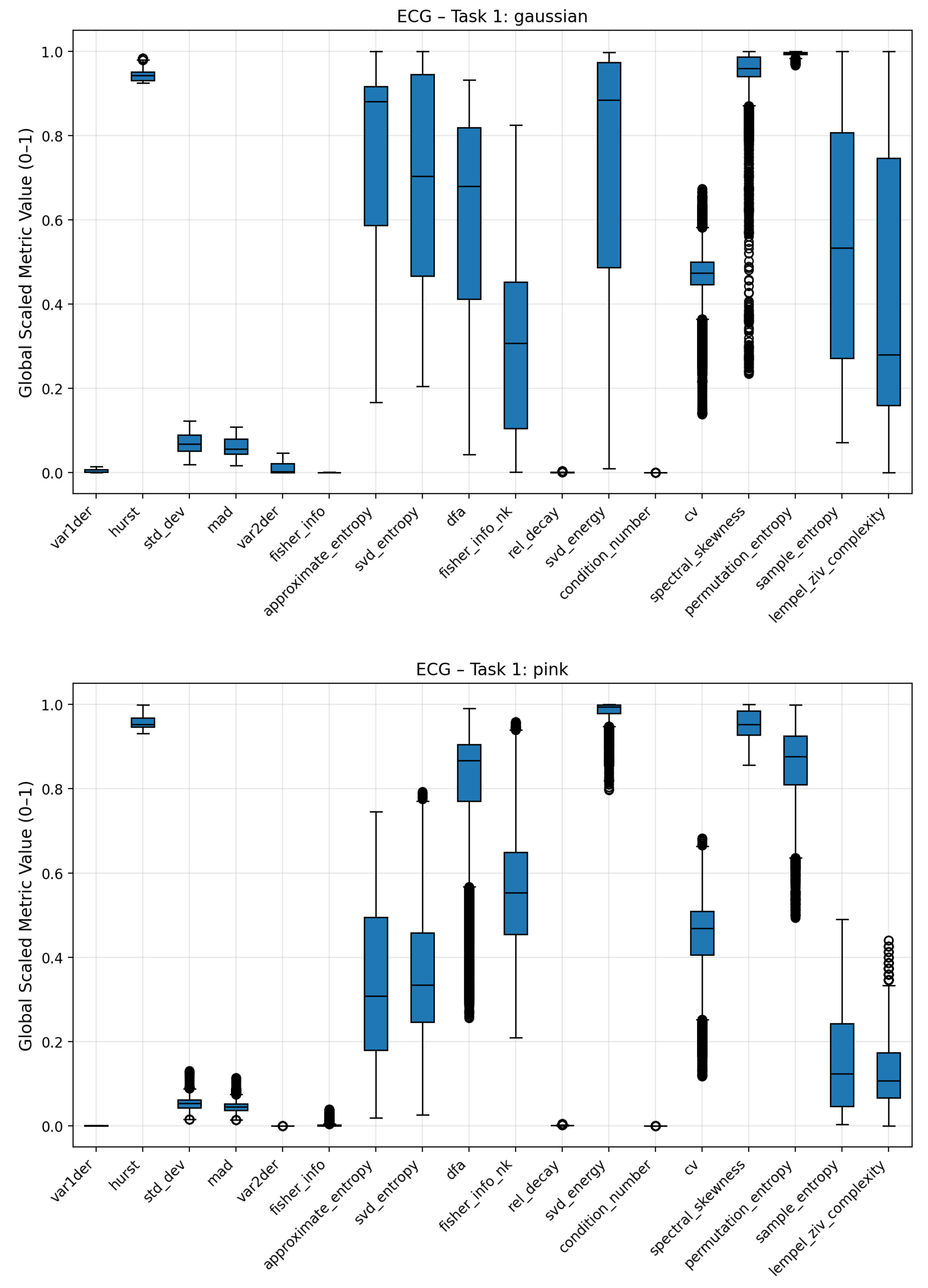
Figure 10.
Boxplots of complexity metrics for the ECG signal under low-frequency drift and no noise. These plots emphasize how structural distortions (low-frequency drift) differ fundamentally from additive stochastic noise. All metrics are scaled between 0–1.
Figure 10.
Boxplots of complexity metrics for the ECG signal under low-frequency drift and no noise. These plots emphasize how structural distortions (low-frequency drift) differ fundamentally from additive stochastic noise. All metrics are scaled between 0–1.
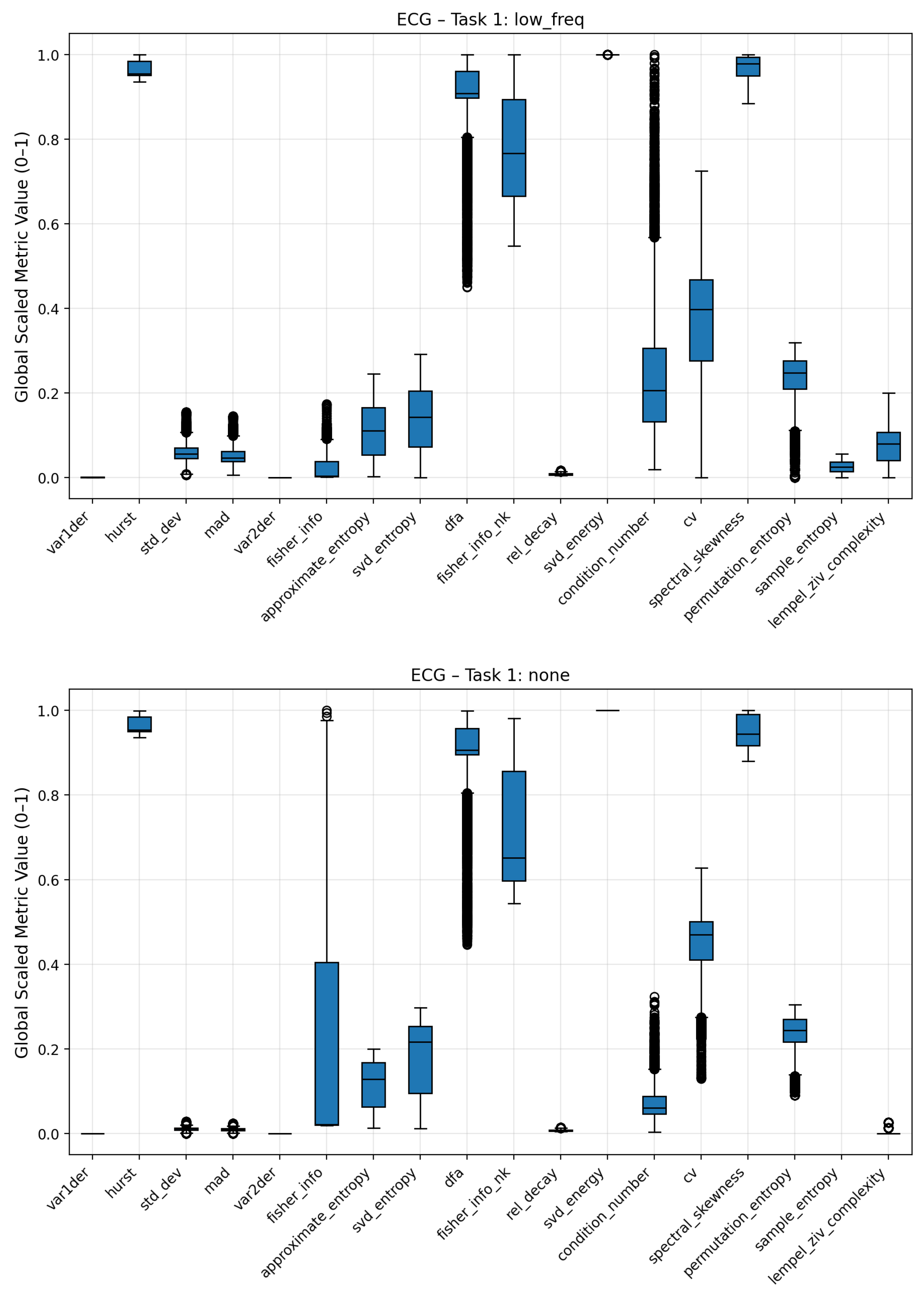
Figure 11.
Average trajectories of complexity metrics for ECG signals across noise intensities.
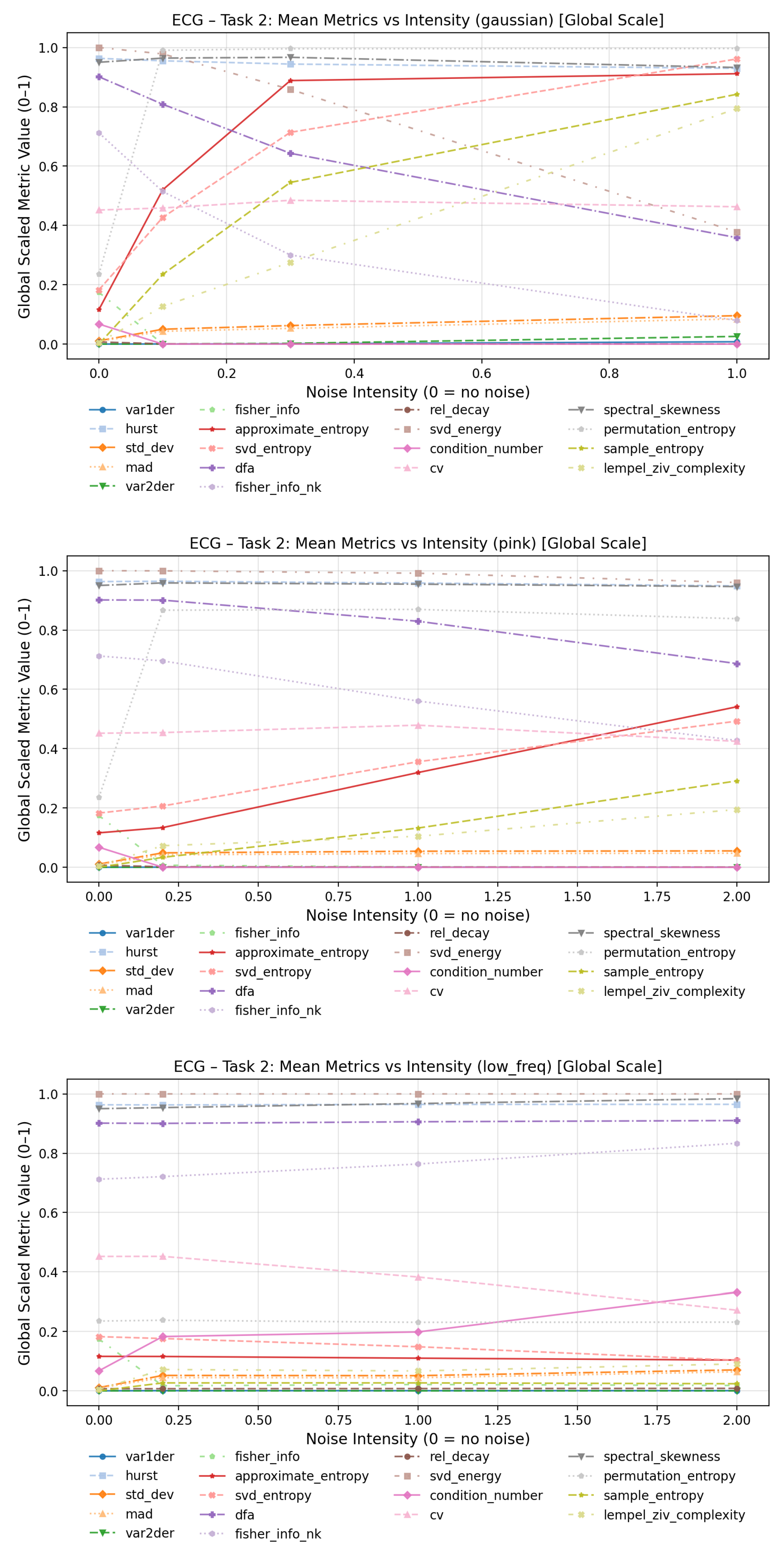

Table 1.
Overview of 18 complexity metrics used in this study and their corresponding data representations. Metrics computed on the phase-space embedding operate on the reconstructed attractor with embedding dimension , time delay , and segment length .
Table 1.
Overview of 18 complexity metrics used in this study and their corresponding data representations. Metrics computed on the phase-space embedding operate on the reconstructed attractor with embedding dimension , time delay , and segment length .
| Metric Category | Metric Name | Data Domain |
|---|---|---|
| Entropy-based | Approximate Entropy (ApEn) [19] | Raw signal |
| Sample Entropy (SampEn) [20] | Raw signal | |
| Permutation Entropy (PE) [21] | Raw signal | |
| SVD Entropy [22] | Embedded matrix | |
| Fractal / Attractor | Detrended Fluctuation Analysis (DFA) [23] | Raw signal |
| Hurst Exponent [24] | Raw signal | |
| Largest Lyapunov Exponent [25] | Embedded Matrix | |
| Statistical | Standard Deviation, MAD, CV | Raw signal |
| Fisher Information (time-domain) [26] | Raw signal | |
| Fisher Information (spectral) [10] | Embedded matrix | |
| Variance of Derivatives (, ) [27] | Embedded matrix | |
| SVD-based/Spectral | Relative Decay of Singular Values [28] | Embedded matrix |
| SVD Energy () [29] | Embedded matrix | |
| Condition Number [30] | Embedded matrix | |
| Spectral Skewness [31] | Embedded matrix |
Table 2.
Average classification performance for the Noise Category Classification task across all systems.
Table 2.
Average classification performance for the Noise Category Classification task across all systems.
| System | Accuracy | Precision | Recall | F1-Score |
|---|---|---|---|---|
| Lorenz | 1.000 | 1.000 | 1.000 | 1.000 |
| Rössler | 1.000 | 1.000 | 1.000 | 1.000 |
| ECG | 0.999 | 0.999 | 0.999 | 0.999 |
Table 3.
Average classification performance for the Noise Category + Intensity Classification task across all systems.
Table 3.
Average classification performance for the Noise Category + Intensity Classification task across all systems.
| System | Accuracy | Precision | Recall | F1-Score |
|---|---|---|---|---|
| Lorenz | 1.000 | 1.000 | 1.000 | 1.000 |
| Rössler | 1.000 | 1.000 | 1.000 | 1.000 |
| ECG | 0.887 | 0.899 | 0.887 | 0.886 |
Table 4.
Average classification performance for the Noise vs. No-Noise Category Classification task across all systems.
Table 4.
Average classification performance for the Noise vs. No-Noise Category Classification task across all systems.
| System | Accuracy | Precision | Recall | F1-Score |
|---|---|---|---|---|
| Lorenz | 1.000 | 1.000 | 1.000 | 1.000 |
| Rössler | 1.000 | 1.000 | 1.000 | 1.000 |
| ECG | 1.000 | 1.000 | 1.000 | 1.000 |
Disclaimer/Publisher’s Note: The statements, opinions and data contained in all publications are solely those of the individual author(s) and contributor(s) and not of MDPI and/or the editor(s). MDPI and/or the editor(s) disclaim responsibility for any injury to people or property resulting from any ideas, methods, instructions or products referred to in the content. |
© 2025 by the authors. Licensee MDPI, Basel, Switzerland. This article is an open access article distributed under the terms and conditions of the Creative Commons Attribution (CC BY) license (http://creativecommons.org/licenses/by/4.0/).
Copyright: This open access article is published under a Creative Commons CC BY 4.0 license, which permit the free download, distribution, and reuse, provided that the author and preprint are cited in any reuse.


