1. Introduction
Existing numerical weather prediction (NWP) adequately depicts large-scale background features of extreme weather events [
1], but is limited by complex dynamic/physical processes and insufficient observations [
2], so its spatiotemporal refined forecasting capability for extremes (e.g., the Zhengzhou “7.20” rainstorm) is restricted [
3,
4]. In particular, China Meteorological Administration (CMA) Fengyun (FY) geostationary satellite atmospheric motion vectors (AMVs) provide quasi-real-time mid- to upper-level atmospheric state data and have become a routine NWP data source that positively influences large-scale backgrounds in global and regional NWP [5-8]. However, AMV retrieval depends on the accuracy of cloud detection and height assignment, and its spatiotemporal error characteristics are complex [9-14], which makes representative-error estimation in real time difficult and leaves the improvement effect on quasi-real-time regional high-resolution NWP unclear [
15,
16]. Therefore, developing an assimilation scheme that accounts for spatiotemporal scale differences and enhances AMV usage efficiency to improve regional NWP holds significant scientific meaning and application value for advancing local complex-weather forecasting and disaster prevention and mitigation.
Initially, AMVs are derived by tracking clouds and moisture gradients in geostationary imagery and are used mainly in the tropics and mid-latitudes, whereas polar orbiters serve high latitudes [
17,
18]. Assuming that AMVs represent horizontal and vertical means of real winds [
19], by introducing high-vertical-resolution satellite observations to strengthen cross-validation of AMVs in assimilation, the difficulty of estimating AMV systematic error can be indirectly reduced, and the generalized application level of overall satellite observations is significantly enhanced, so 3D schemes that fuse AMVs and hyperspectral satellite observations receive wide attention [
17,
20,
21]. For example, introducing high-vertical-resolution wind profiles from the European Space Agency (ESA) Aeolus Doppler wind lidar (DWL) notably improves global NWP wind fields [
22] and tropical cyclone forecasts [
23]; introducing high-vertical-resolution observations from the CMA FY3D Microwave Humidity Sounder (MWHS-II) and/or FY4A Geostationary Interferometric Infrared Sounder (GIIRS) positively affects global NWP temperature, humidity, and winds [
24] as well as tropical cyclone forecasts [
25]. However, current limitations of AMVs and/or satellite hyperspectral observations in cloudy regions [
9,
20,
26], together with nonlinear approximations in assimilation and conflicts with model-resolvable scales [
21,
27,
28], highlight the necessity-beyond new satellite technologies [
29]-of developing suitable AMV application schemes to address complex regional weather challenges [
17].
Three-dimensional variational (3DVar) assimilation is currently applied in regional high-resolution models of every NWP center for its efficient multi-platform observation merging [
30,
31]. It remains challenged by background error covariance accuracy, model error, strong atmospheric nonlinearity, and difficulty in estimating representative errors of unconventional observations [
32,
33]. Specifically, advantages of FY geostationary AMV Var assimilation in large-scale systems [5-8] and its deficiencies in meso- to small-scale forecasts [
15,
16] indicate that current Var representative-error estimates, which treat different AMV data as a single observation type, underestimate spatiotemporal differences among channels and/or variables. Thus, solely adjusting AMV representative errors to raise observation usage in regional high-resolution Var assimilation, while underestimating spatiotemporal errors among different AMVs, yields limited improvement in forecasting regional complex weather events.
Early real-time scattered nudging assimilation (also known as four-dimensional data assimilation or FDDA) of NESDIS GOES winds shows small yet stable positive impacts on mesoscale NWP analyses and forecasts [
34]. Nudging offers low computational cost and few parameters versus four-dimensional variational and ensemble Kalman filter [
35,
36], yet it updates NWP local states independently using compared observation [
37,
38] and remains sensitive to observation density [
39]. FDDA receives wide attention in multi-scale NWP models [
40,
41] and high-frequency updating models with massive observations [
42,
43]. Limited by existing frameworks, the effectiveness of FDDA schemes with geostationary AMVs for regional complex weather and their comparison with Var schemes remain to be investigated.
In general, FY4A AMVs exhibit high temporal but low spatial frequency, and inter-channel differences are pronounced [
44,
45]. Their applications in existing numerical systems differ markedly, e.g., large-scale Nudging versus direct high-resolution 3DVar assimilation, and their impact on regional severe-weather forecasting remains unclear. To address this, combined the three-channel merged AMVs (3D-winds hereafter) with a multi-scale (12-, 4-, and 1-km) NWP model, the NFV scheme that updates the large-scale forcing of the finer-scale 3DVar is designed. Ablation experiments between Nudging and 3DVar assimilation are conducted for the Zhengzhou “7.20” extreme-rain event to clarify their respective impacts on FY4A 3D-winds assimilation and nowcasting, aiming to improve numerical nowcasting schemes of geostationary 3D-winds.
2. Data and Model
2.1. Data
2.1.1. Observation
Based on FY4A AMVs [
44,
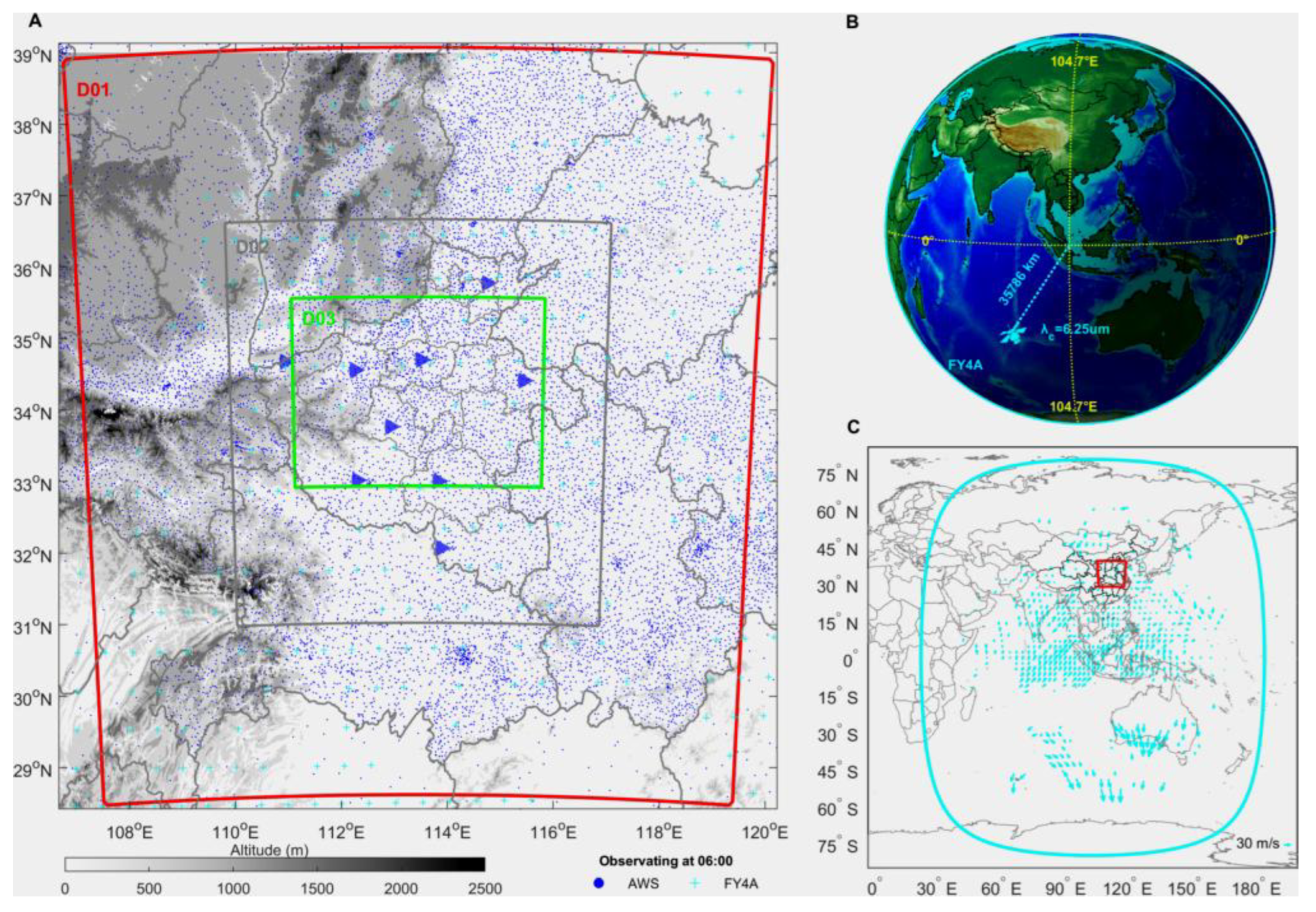
45] from CMA National Satellite Meteorological Center (NSMC), horizontal winds of low-level water-vapor ch09 (6.95μm), high-level water-vapor ch10 (7.42μm) and infrared ch12 (10.7μm) are quality-controlled and merged into FY4A 3D-winds profiles, which has 3-h and around 48-km resolution and is used for assimilation and forecasting. It is distributed over northern Henan and surrounding cloudy areas at UTC 06:00 before the Zhengzhou “7.20” rainstorm (
Figure 1A, cyan crosses). FY4A carries the Advanced Geostationary Radiation Imager (AGRI, on-orbit parameters in
Figure 1B) with 14 channels covering 0.5~15 μm at 1-h resolution; AMVs are derived from its successive images, and ch09 cylindrical projection and study area are shown in
Figure 1C. Besides AMVs, FY4A black-body brightness-temperature (TBB) product [
46] at 1-h and 4-km resolution is collected to verify assimilation impacts on mid- to upper-level TBB forecasts.
Moreover, the surface automatic weather station observation (AWS), CMA Land Data Assimilation System reanalysis datasets (CLDAS), and nine S-band Doppler Radar data (
Figure 1A) derived from the CMA Henan Meteorological Bureau are collected for nowcasting indicator verification over D03 domain. The AWS with a resolution of around 0.1° and 1-h intervals accounts for hourly rainfall evaluation, while regarding AWS's discontinuities, the CLDAS with a resolution of around 0.05° and 1 h intervals accounts for total rainfall evaluation. The nine Radar reflectivity data with a bin-width length of around 230 m, 6 min intervals and 11 elevation numbers, are firstly quality controlled with various clutter and range suppression checks for each radar, then remapped with 0.01° grids for each elevation number, and finally the maximum reflectivity across 11 elevation numbers for each grid is taken as the composite reflectivity (briefed as CR hereafter), which accounts for the convection evaluation.
2.1.2. Forcing
The atmospheric forcing datasets are collected from the first-generation global atmospheric/land-surface reanalysis project (CRA40), which has a resolution of 34-km and 64 pressure levels, and 6-/3-h intervals for atmospheric/surface layer [
47,
48]. Meanwhile, the Noah LSM driven by the NASA's Global Land Data Assimilation System reanalysis (GLDAS) has a resolution of 0.25°, 3-h, and 4-layer. The USGS' SRTM 3s DEM and the NASA's MODIS 5s land cover datasets are used as the WRF's underlying terrain and land cover, respectively. Moreover, due to the computation and storage limits, the lighter FNL data (i.e., 0.25°, 6-h, and 27-layer) is collected to assemble the 3DVar’s background errors between 12h- and 24h-lead forecasts using the month-long initial-time-differed forecasts (known as NMC method).
2.2 WRF
The WRF model (version 3.9.1) is employed in this study to simulate the regional rainstorm event. The model uses nested domains with one-way feedback, that only considering the feedback from outer to inner domains. The outer and middle domains are both centered at 113.45°E, 33.85°N, and consist of 100×100 grids at 12-km resolution and166×160 grids at 4-km resolution respectively, and the inner domain is centered around Zhengzhou city, and consists of 301×201 grids at around 1-km resolution. The model includes 51 levels with 11 levels below 1 Km, and the model top pressure is 50hPa. The time integration step is 30 seconds.
For the outer domain, the Kain-Fritsch (KF) convection scheme [
49] is used, while convection is turned off in the inner domain. Other physical processes are modeled using the same schemes for both domains: the Thompson scheme for cloud microphysics [
50], the Yonsei University (YSU) scheme for boundary layer physics [
51], the Rapid Radiative Transfer Model (RRTMG) scheme for both long-wave and short-wave radiation physics [
52], the Monin-Obukhov similarity scheme for surface physics [
53], the Noah Land Surface Model (LSM) scheme for land surface physics [
54], and the Unified Canopy Model (UCM) scheme for canopy physics [
55].
3. Method
3.1. Assimilation
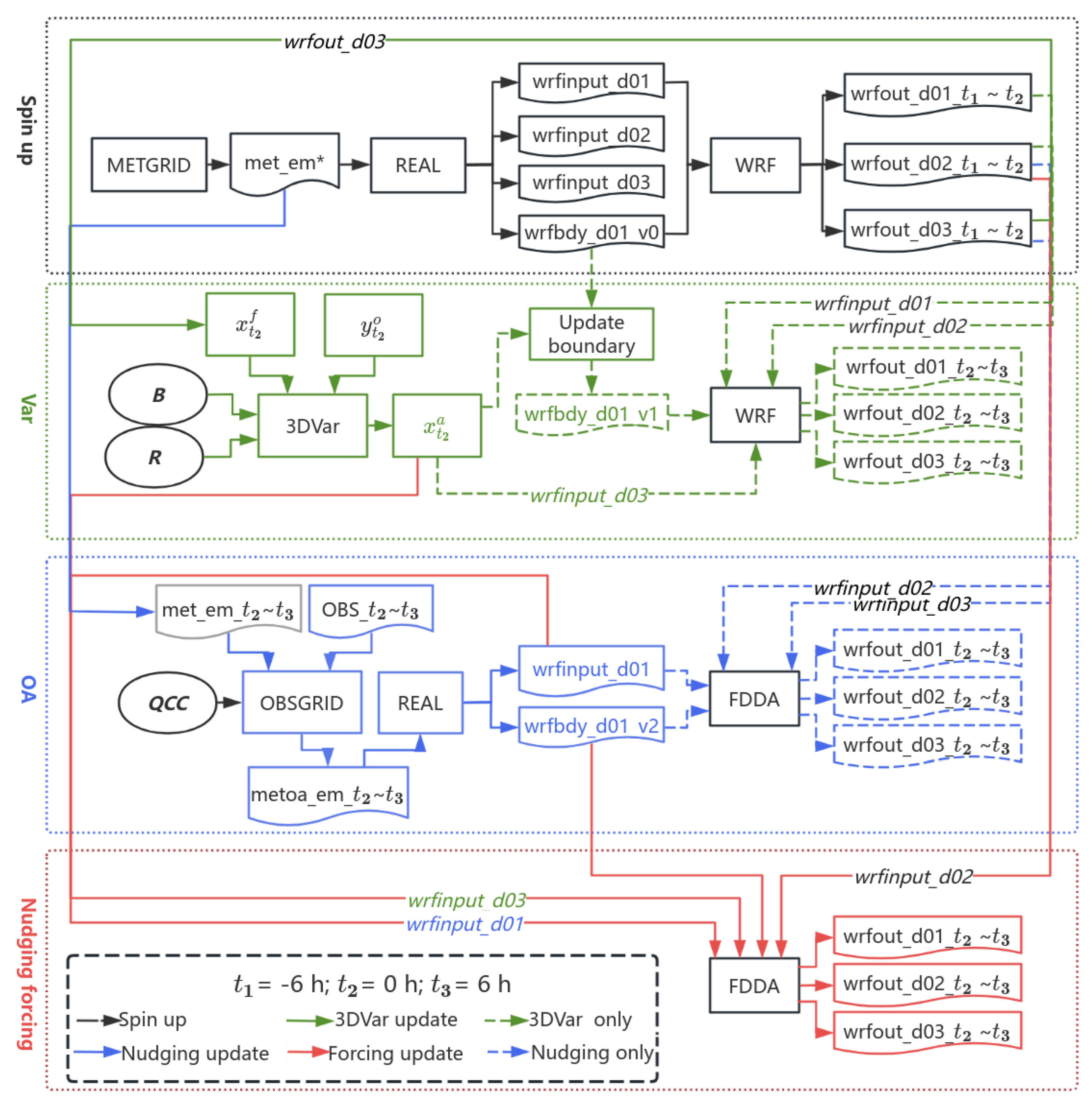
As shown in
Figure 2, the NFV scheme is based on WRF 3DVar (green solid line) for high-resolution assimilation [
56], and is driven by large-scale Nudging through objective analysis (briefed as OA hereafter; blue solid line) and FDDA (red solid line), completed in four steps.
First, use forcing data to drive WRF for cold-start spin-up; met_em* files and the -6~0h forecast (~) are generated. Second, Var update uses the 0 h () spin-up forecast as background (), ingests observations(), and updates the background using background and observation covariance (i.e., and ) to yield an analysis . Third, OA update uses the 0~6h (~) spin-up met_em* sequence as background, continuously ingests concurrent observations (OBS_~) with QCC, and produces OA sequence (metoa_em*) that initializes new D01 initial and boundary conditions. Finally, in Nudging forcing, the spin-up forecast and supply initial conditions for D02 and D03, respectively; WRF FDDA continuously updates the D01 fields, yielding the NFV 0~6h (~) forecast. Details of Nudging in NFV are detailed in section S1.1 of the Supplements.
Note that Var and Nudging run separately over different domains and simultaneously without extra cost; independent forward integrations with spin-up data provide single-scheme ablation forecasts in NFV (
Figure 2, dashed lines).
QCC is an integer flag derived from an observation-preprocessing quality-control scheme that includes limb, background, temporal-spatial, and physical consistency checks. Observations with
QCC > 2
10 are rejected in both Nudging and Var, constituting observation quality control for FY4A 3D-winds. Quality-controlled observations are subsequently used for verification and evaluation. In 3DVar,
adopted the NMC method using FNL data-driven forecasts,
chose the global sounding climatological errors, and the observation innovation as observation-minus-background (OMB) greater than
is rejected.
3.2. Verification
To verify the impacts of Nudging and Var in the NFV method, linear fitting and multiple objective metrics are applied in observation space. These metrics include root-mean-square error (RMSE), mean absolute error (MAE), correlation coefficient (CC), goodness-of-fit (R²) and so on (detailed in S1.2.1 section). Element-wise comparisons are performed at FY4A observation points for observations, background, and analysis. Differences in background between OA and 3DVar domains and resolutions are considered. In model space, primary features of analysis-minus-background (AMB) for observed variables are compared.
To verify NFV impacts on forecasts, linear fits and metrics (as
RMSE,
MAE,
CC and
R²) for FY4A 3D-winds and forecasts are compared. By using the Radiative Transfer model for TOVS (RTTOV, v14) [
57], the forecast TBB are retrieved (see section S1.2.2) and further compared with FY4A TBB data. Especially, based on the fine observations as AWS, CLDAS, and Radar CR, comprehensive validations as the probability density function (PDF) fitting, the Roebber skills [
58], and the Method for Object-based Diagnostic Evaluation (MODE) metrics [
59] are conducted for the key nowcasting indicators over D03 domain, i.e., short-duration heavy rain (briefed as SHR hereafter), 6-h rainstorm, and severe convection. Note that SHR is defined as the hourly rainfall exceeding 25 mm, 6-h rainstorm is defined as rainfall exceeding 50 mm, and severe-convection is defined as CR exceeding 45 dbz. To ensure an equatable verification, the forecasts and observations are all regridded into identical grids of 0.01° with bilinear interpolation. Also, the convolution radius is twice the grid resolution for SHR and 6-h rainstorm, while 20 times the grid resolution for severe-convection.
Finally, spatial differences between Nudging and Var forecasts, such as
RMSVD,
VCC,
VR² and so on (see section S1.2.1), are compared. Rotunno-Klemp-Weisman (short for RKW hereafter) environmental conditions [
60,
61] are analyzed to clarify how FY4A 3D-winds assimilation influences NFV nowcasting through unobserved mesoscale systems and thermodynamic conditions during this rainstorm.
4. Experiment
Experiments CTR, NFV, 3DVar, and Nudging are designed (
Table 1) for 06:00~12 :00 UTC 20 July 2021, covering the whole Zhengzhou “7.20” rainstorm period. CTR supplies the background for assimilation. In NFV, FDDA (D01) and 3DVar (D03) assimilate all FY4A 3D-winds variables (P, T, U, V); quality control applies
QCC and R (see section 3.1), and serves as the reference. Experiments Var and Nudging are obtained by removing FDDA and 3DVar assimilation from NFV, respectively, thus providing mutual method ablation of NFV.
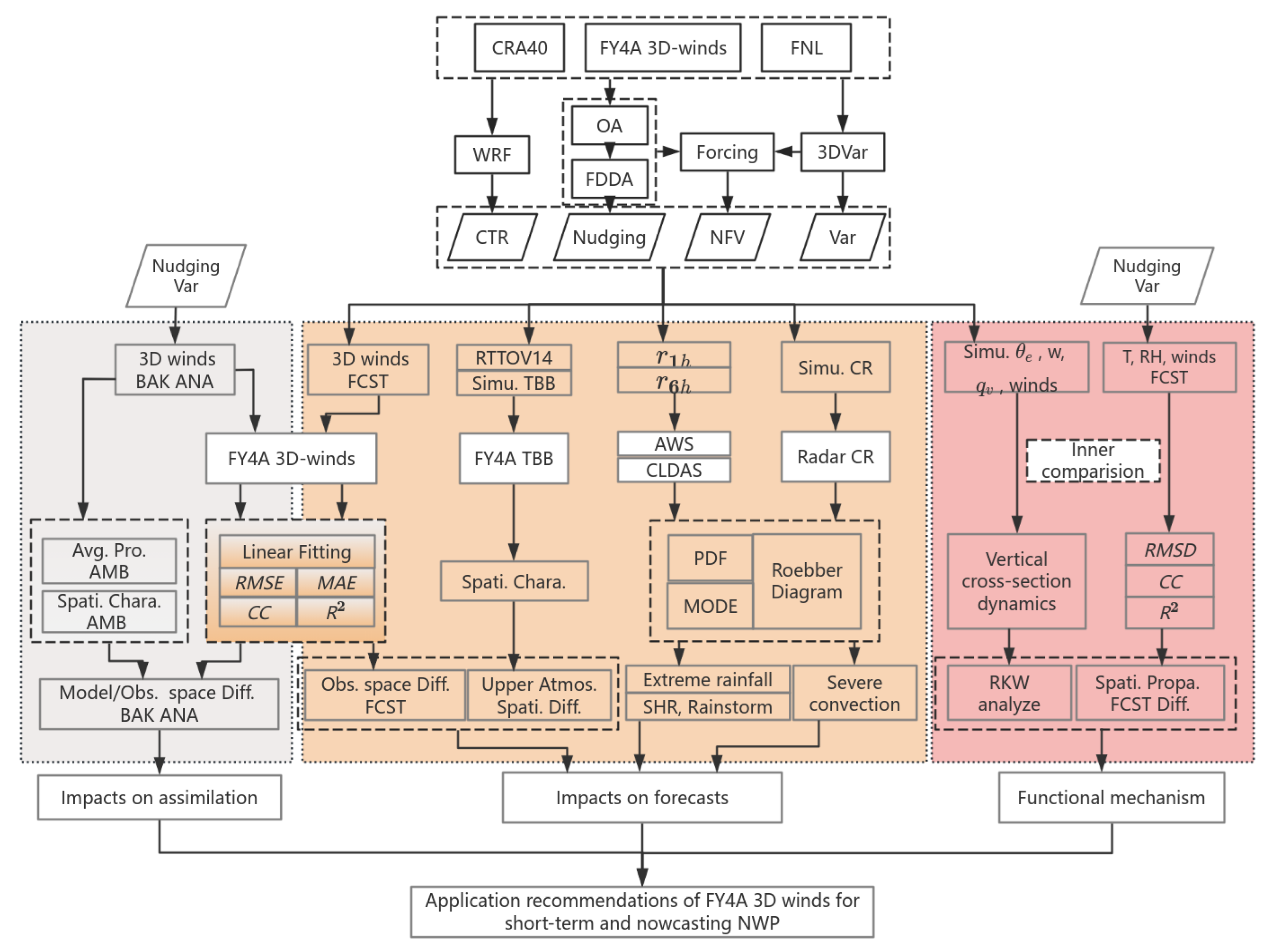
The research flow comprising main three steps is shown in
Figure 3. First, multi-index comparisons of observation, background, and analysis in observation space from Var and Nudging simulations quantify observational impacts within NFV. Second, verification of forecasts against observations in observation space, comparison of RTTOV14 retrievals with FY4A observations, and precipitation and convection diagnostics identify the principal forecast influenced by FY4A observations. Third, analysis of forecast error propagation and differences in RKW environmental conditions between Var and Nudging outputs elucidates the synoptic mechanisms by which FY4A observations induce forecast differences. Recommendations for the numerical nowcasting application of FY4A AMVs are ultimately provided.
5. Results
5.1. Impacts on Assimilation
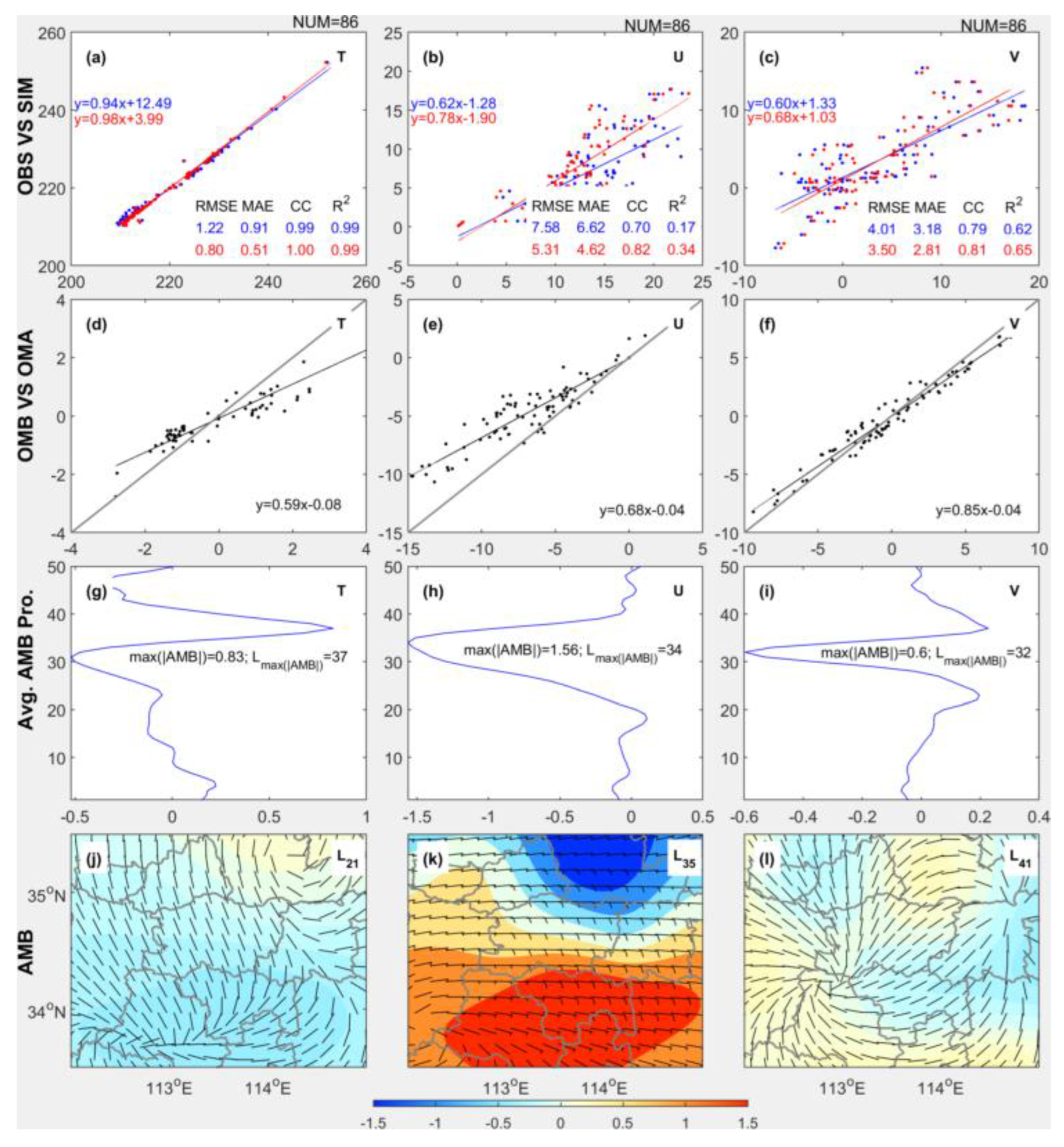
5.1.1. 3DVar
Figure 4 presents the combined comparison of observations, background, and analysis for 3DVar. For the linear fit between OBS and SIM, 86 full-observation pairs (T, U, and V) enter assimilation; ANA fit coefficients are closer to 1 than BAK, while
RMSE and
MAE decrease and
CC and
R² increase (
Figure 4a~c). For linear fits of OMB and OMA, coefficients are both below 1 (
Figure 4d~f). These indicate clear positive impacts of 3DVar assimilation on T, U, and V in observation space. For domain-averaged AMB profiles, maximum absolute values of T, U, and V are 0.83 K, 1.56 m/s, and 0.6 m/s, respectively, concentrated between model layers 30~40 (
Figure 4g~i). AMB increments for temperature and wind are weak at layer 21 and 40 but relatively strong at layer 35, showing overall warm-easterly characteristics (Fig. 4j~l). This indicates that assimilation significantly adjusts the mid-upper levels (around 400~200 hPa) of BAK, exhibiting divergence with lower-level cooling, upper-level warming, and southeast-wind.
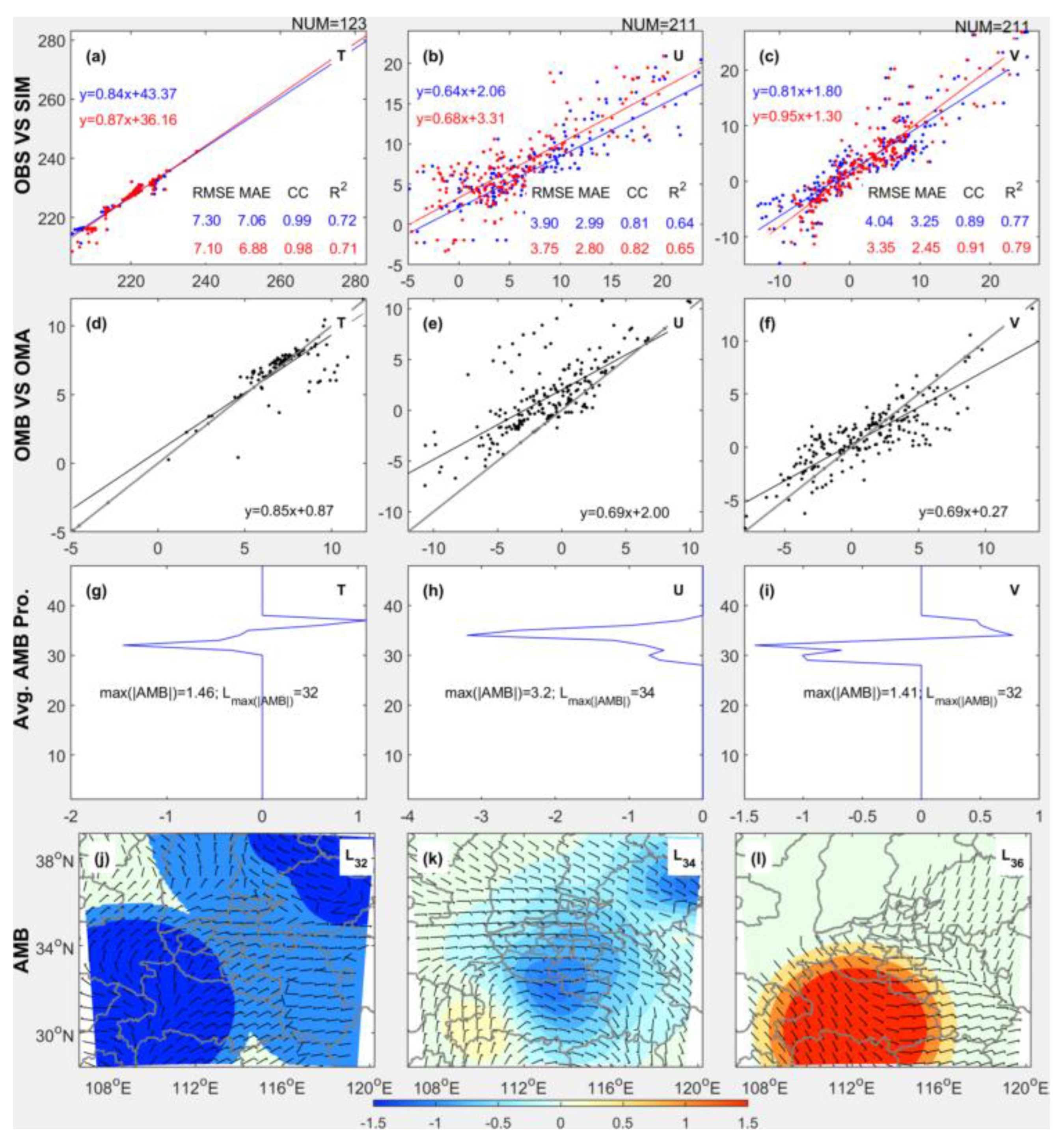
5.1.2. OA
Figure 5 compares OA observations with background and analysis at 06 UTC. For OBS-versus-SIM linear fits, 123 T, 211 U and 211 V samples are assimilated; ANA fit coefficients improve and
RMSE and
MAE decrease (
Figure 5 a~c). OMB and OMA linear fits both yield coefficients below one (
Figure 5 d~f), indicating clear positive OA impacts on T, U and V in observation space. Domain-averaged AMB profiles show maximum absolute values of 1.46 K, 3.2 m/s and 1.41 m/s for T, U and V respectively, all concentrated between model layers 30-40 (
Figure 5 g~i). AMB exhibits cold anomaly, easterly wind and warm anomaly at layers 32, 34 and 35, respectively (
Figure 5 j~l). These results demonstrate that OA significantly adjusts the mid-upper levels (around 400~200 hPa) of BAK, characterized by lower-level cooling, upper-level warming and southeast-winds enhancement.
OA at 09 and 12 UTC performs similarly to 06 UTC, with slightly increased observation counts (see Figures S2). Compared with 3DVar, OA assimilates significantly more observations. Mid-upper AMB patterns resemble those in 3DVar but are markedly stronger in OA. Thus, within NFV, OA continuously adjusts D01 mid-upper temperature and wind toward observations, exhibiting persistent pronounced divergence increments, whereas 3DVar effectively improves D03 mid-upper fields with weaker divergence increments.
5.2.Impacts on Forecast
5.2.1. Upper Atmosphere
5.2.1.1. Compared with FY4A Winds
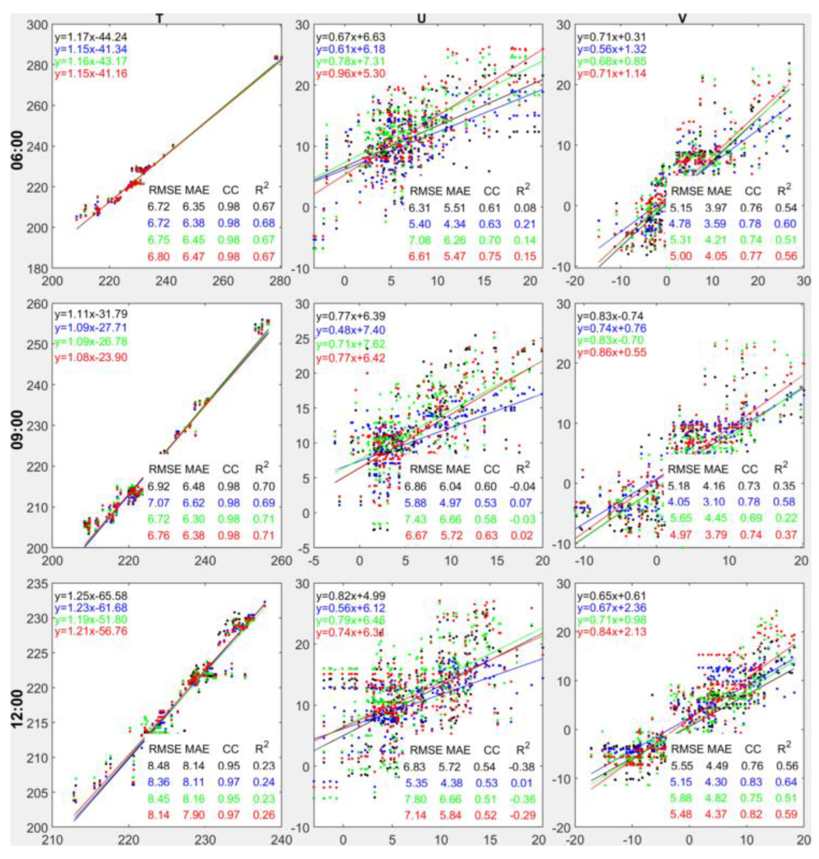
Fitting between forecasts and FY4A 3D-winds are shown in
Figure 6. For T, linear coefficients slightly exceed 1 and intercepts are large, indicating systematic forecast deviation that is most pronounced at 12 UTC. For U and V, coefficients are below 1, indicating adjustment toward observations.
For T, fit coefficients of all assimilation experiments are closer to 1 than CTR, indicating positive assimilation impacts. However, inter-experiment differences in RMSE and MAE remain below 0.5 K, and those in CC and R² below 0.03, revealing limited improvements likely linked to strong upper-level signals such as temperature lapse rates. For U and V, Nudging yields the lowest linear fit coefficients, RMSE and MAE at every forecast time, whereas NFV shows the opposite. This indicates that reduced vector-wind errors in the upper atmosphere demonstrate Nudging's greater positive impact through increased the FY4A 3D-winds assimilation entries, yet its spatial linear-fit capability is significantly weakened. NFV's contrasting performance implies highly nonlinear multi-scale interactions of upper-level vector winds.
5.2.1.2. Compared with FY4A TBB
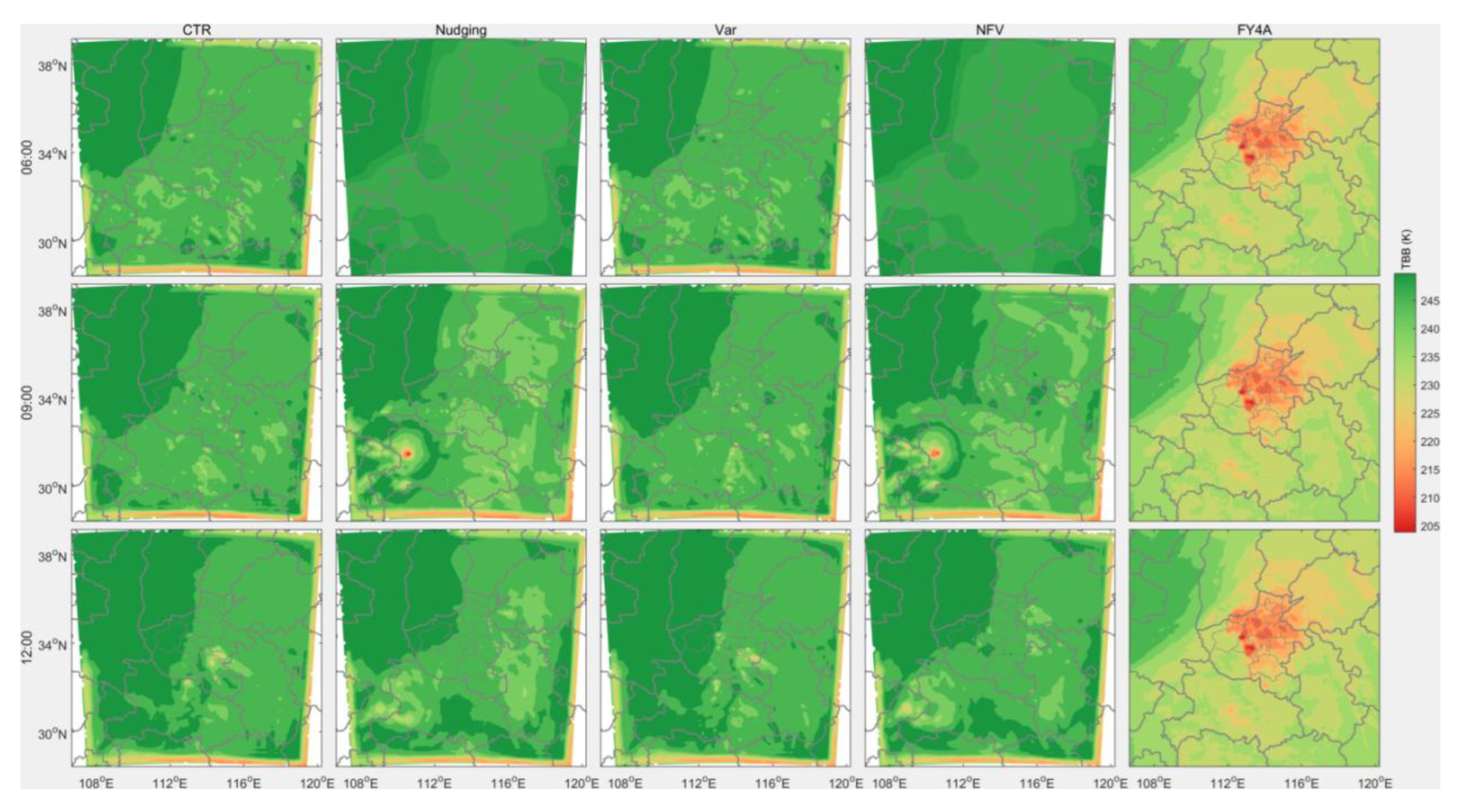
Due to the limited retrieval resolution of the RTTOV14 model, forecasts from the coarser D01 domain are used for RTTOV14 simulations and compared with FY4A ch09 TBB (
Figure 7). Although significant magnitude differences exist, the northeast–high–southwest–low TBB pattern in all experiments agrees well with observations. Notably, compared with CTR and Var, Nudging and NFV better reproduce the observed patchy low-value regions at 09 and 12 UTC.
Overall, FY4A Winds assimilation exerts distinct positive impacts on upper-level forecasts. On one hand, in D03 FY4A Winds observation space, error reduction and increased correlation are seen for Nudging, enhanced vector-wind linear fit for NFV, and intermediate performance for Var. On the other hand, in D01 FY4A ch09 TBB, Nudging and NFV exhibit superior spatial consistency. These likely linked to greater observation ingestion in Nudging and multi-scale interactions across different domains.
5.2.2. Rainfall
5.2.2.1. Probability density distribution
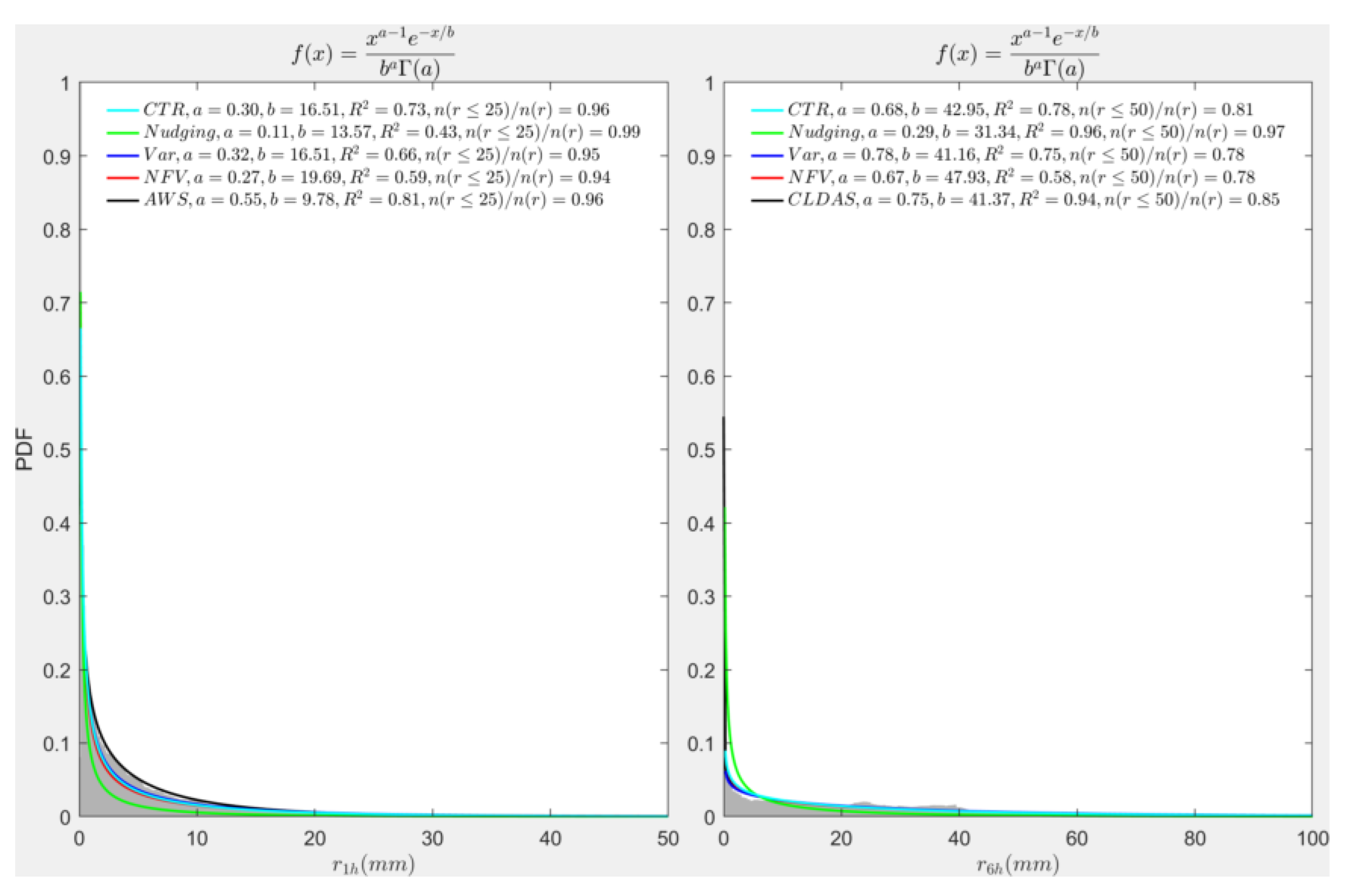
Figure 8 shows the gamma (Γ)-distribution fits of
(about 3.6×10
7 samples) and
(about 6×10
6 samples) within 1,000 bins for all data, whereas all
R² exceeds 0.43, indicating consistent distributions. The shape parameter
for
stays below 0.5 for all data, revealing extreme heterogeneity, whereas
for
exceeds 0.6 except for Nudging, implying more uniform coverage. For
and
, Nudging yields the smallest a and the highest light-rain fraction, denoting highly uneven light precipitation, while NFV exhibits the largest scale parameter
and the lowest light-rain fraction, indicating the greatest mean intensity and frequent heavy rainfall.
5.2.2.2. Roebber Skill Scores
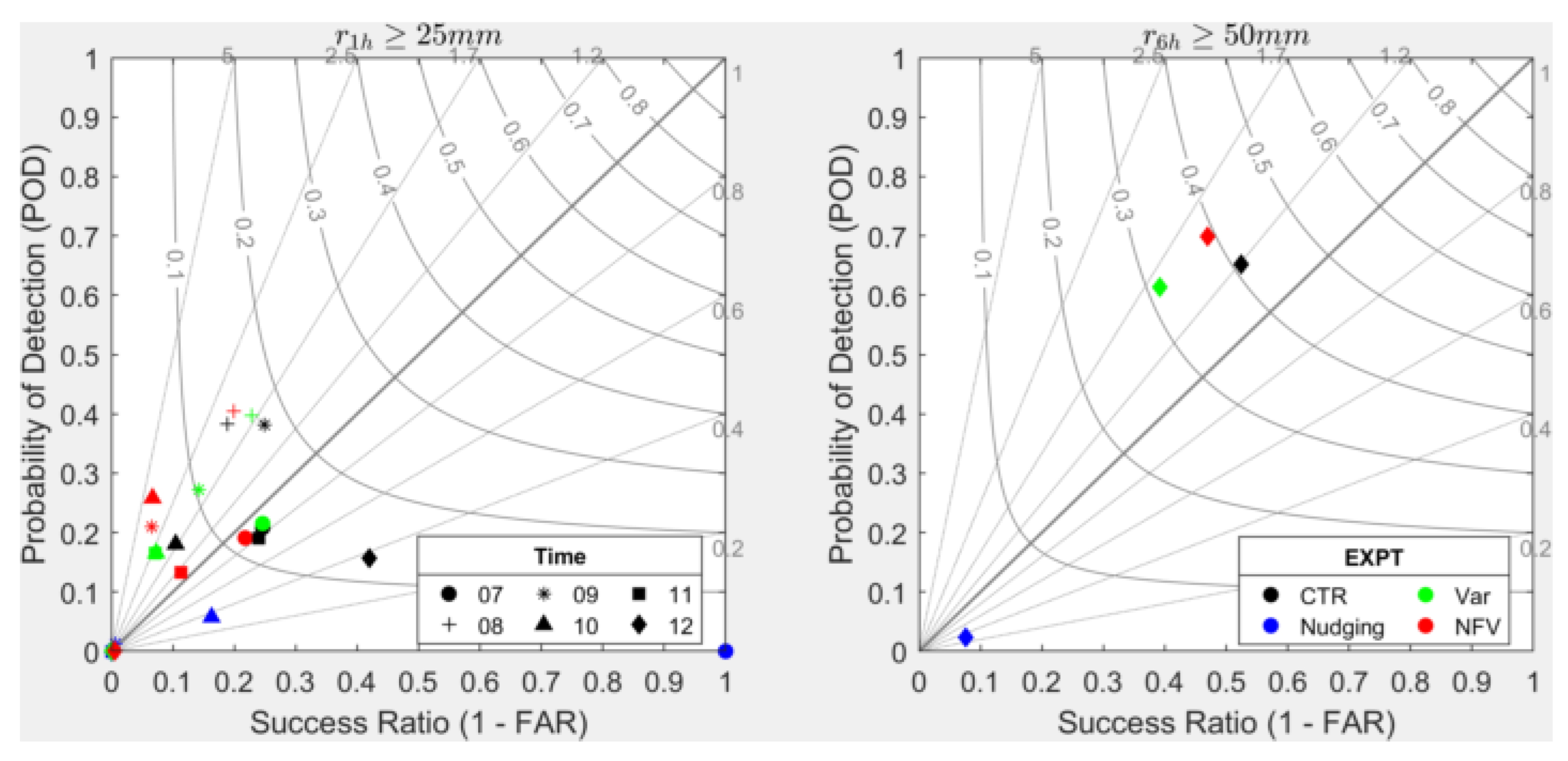
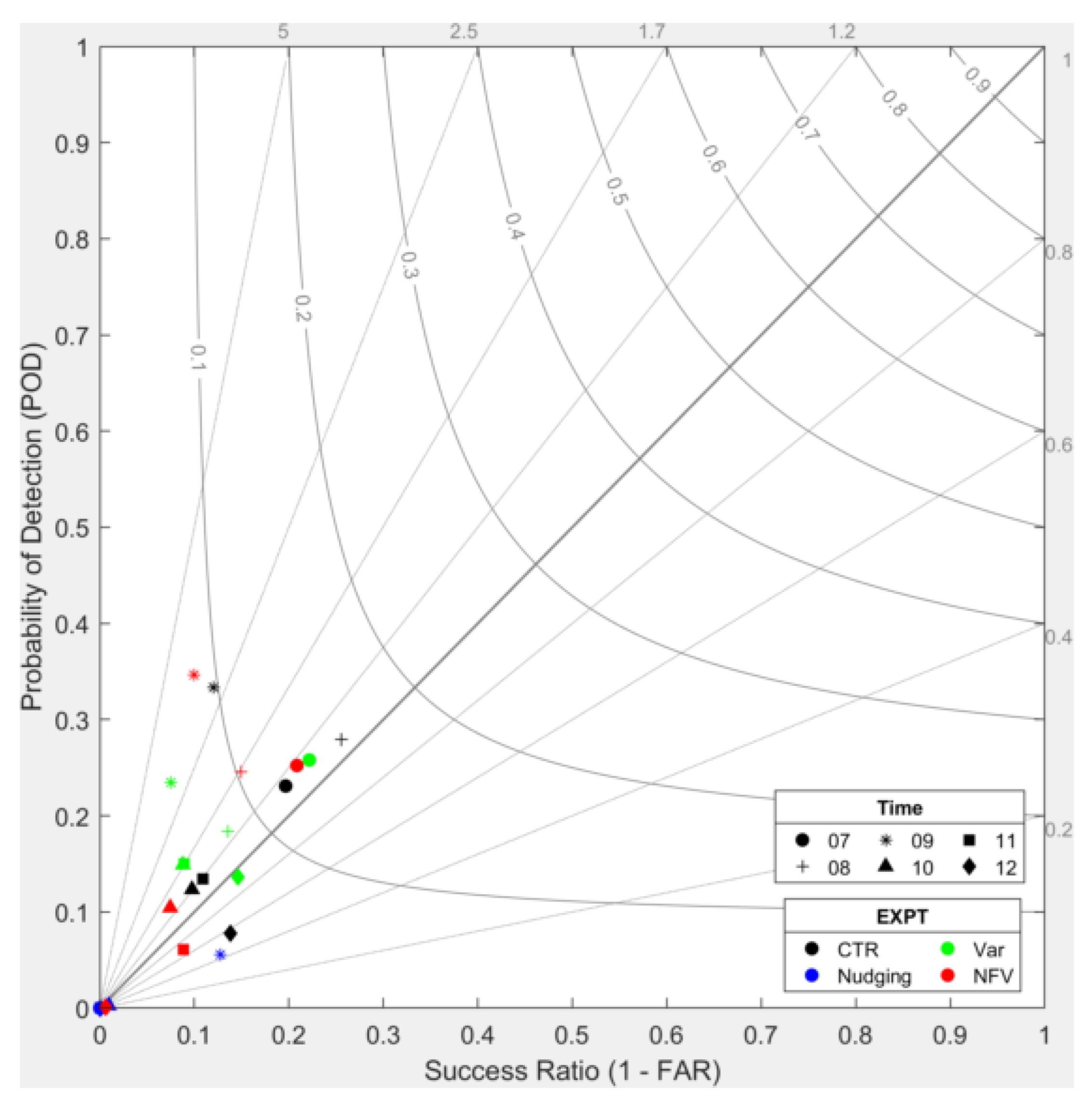
Figure 9 compares comprehensive precipitation skills. For SHR and rainstorm events, most points lie on the upper-left of the Roebber diagram, indicating evident over-forecasting. For SHR in
, except at 08 UTC, the critical success index (CSI) never exceeds 0.1, so skill differences among experiments are indistinguishable. At 08 UTC, NFV yields the highest probability of detection (POD), yet Var attains the highest success rate (SR) and CSI and a BIAS closest to 1, giving the best skill. Consequently, Var ranks first, followed by NFV, CTR, and Nudging last. For rainstorm in
, all experiments except Nudging outperform those for short-duration heavy rain. Specifically, the highest POD is approximately 0.7 (NFV), the highest SR is approximately 0.5 (CTR), the highest CSI is approximately 0.4 (CTR and NFV), and the BIAS is approximately 1.2 (CTR). Thus, CTR exhibits the best skill, followed by NFV, then Var, and Nudging is the worst.
Overall, SHR skill (CSI ≤ 0.2) is markedly lower than rainstorm skill (CSI > 0.3), indicating low skill or poor verifiability. Integrating both types, NFV shows consistent performance, CTR and Var exhibit large uncertainty, and Nudging performs worst.
5.2.2.3 SHR, Extremes and Rainstorm
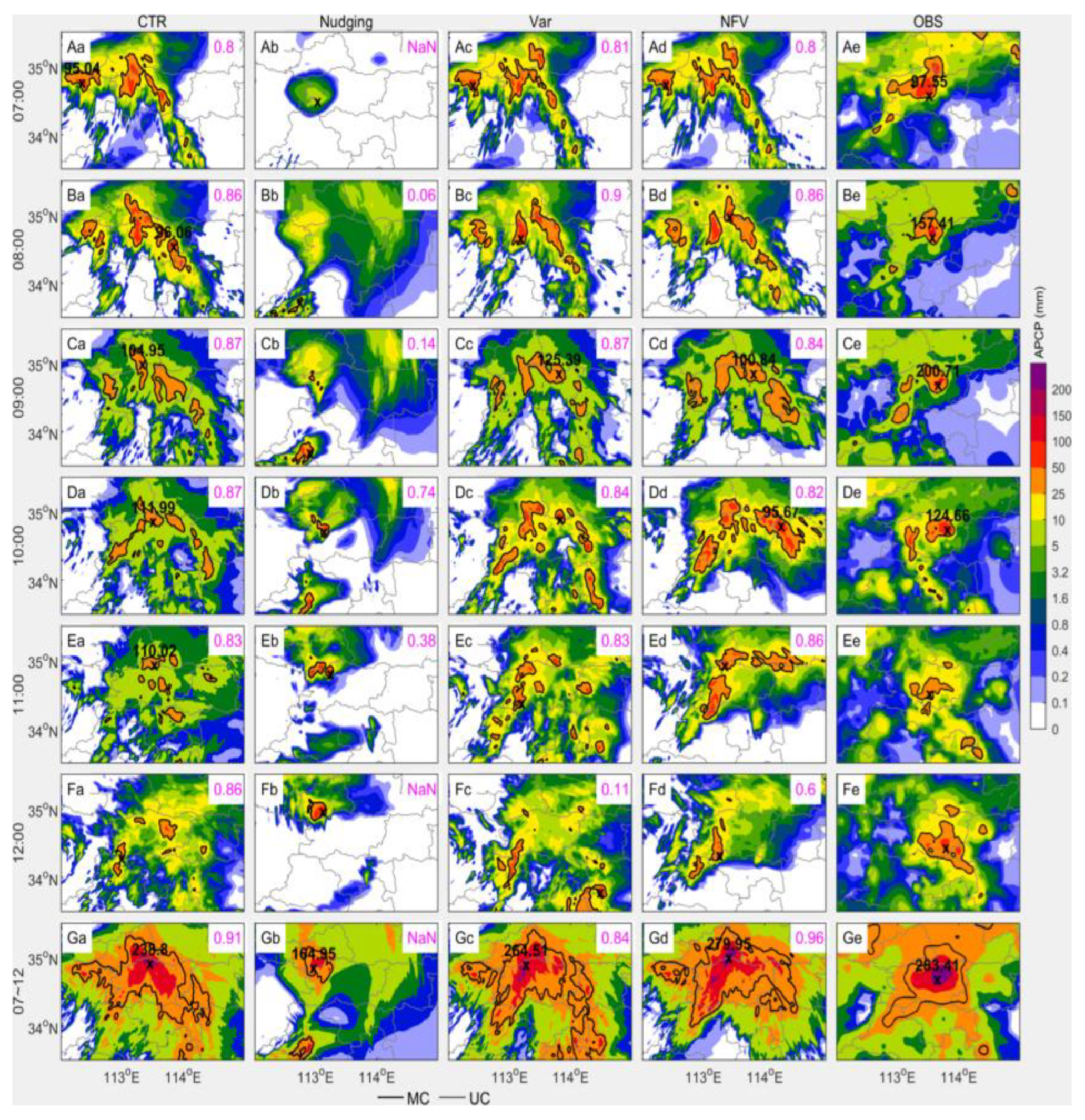
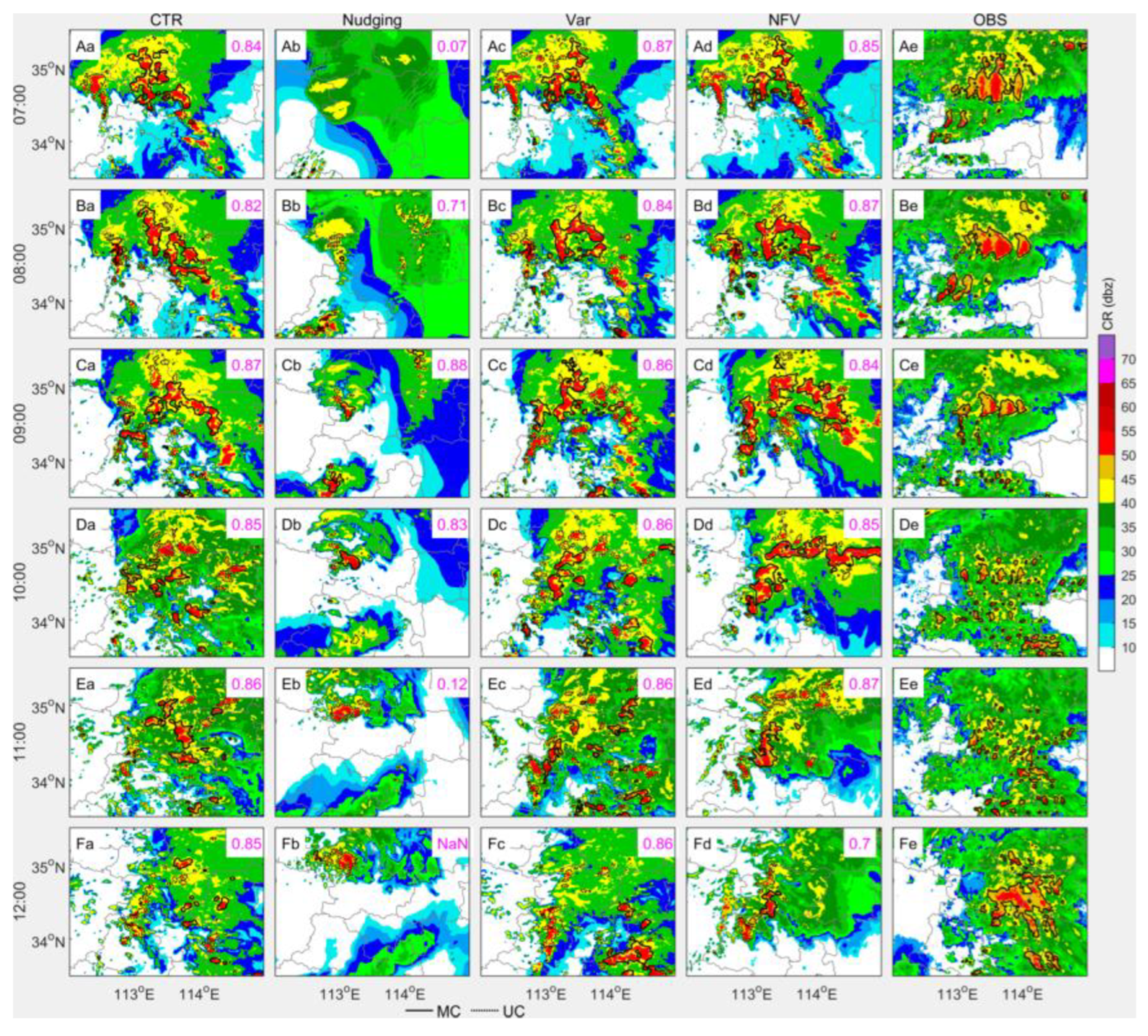
During 07~12 UTC, comparisons of forecast and observed precipitation are shown in
Figure 10 A~F. Observations indicate that SHR regions remains over Zhengzhou (
Figure 10 Ae~Fe). From 07~10 UTC, an extreme point (“x”,
≥95 mm) is observed near downtown Zhengzhou (around 34.6°N, 113.8°E), exceeding 200 mm at 09 UTC (
Figure 10 Ce), after which the SHR weakens, consolidates, and slightly extends southeastward.
at 07~12 UTC 20 July for CTR, Nudging, Var, NFV, and AWS stations; “x” marks extreme points (values shown if ≥95 mm). Black contours in a~e outline MODE objects with threshold ≥25 mm; solid and dashed lines in a~d denote matched (MC) and unmatched (UM) objects, with magenta numbers giving total interest (TI). Panel G is as A~F but for at 12 UTC with object threshold ≥50 mm compared to CLDAS.
During 07~10 UTC, CTR, 3DVar, and NFV produces similar SHR patterns, all larger than observed; the extreme point “x” is shifted north by CTR, while Var and NFV are closest to observations (
Figure 10 Aa~Da, Ac~Dc, Ad~Dd). At 09 UTC, Var's extreme reaches 125 mm (
Figure 10 CC); afterward, their positions diverge and areas shrink below observed. Nudging's SHR area is markedly smaller, confined to western Zhengzhou (
Figure 10 Ab~Fb). The MODE total interest (TI) for SHR is valid only at 10 UTC for Nudging (0.74). CTR, Var, and NFV achieve TI above 0.8 during 07:00~11:00 UTC, indicating good spatial features, but Var's TI drops sharply to 0.11 at 12 UTC, revealing pronounced spatial error.
Figure 10 G shows that observed
precipitation at Zhengzhou center reaches 283 mm; NFV simulates about 280 mm but slightly north, while other experiments produce maxima below 250 mm and positions shifted west. MODE TI for rainstorm indicates NFV attains the highest TI (0.96), demonstrating the best spatial pattern among all schemes. Nudging exhibits missed events, and Var shows evident false alarms.
5.2.2.4 Spatial Object Characteristics
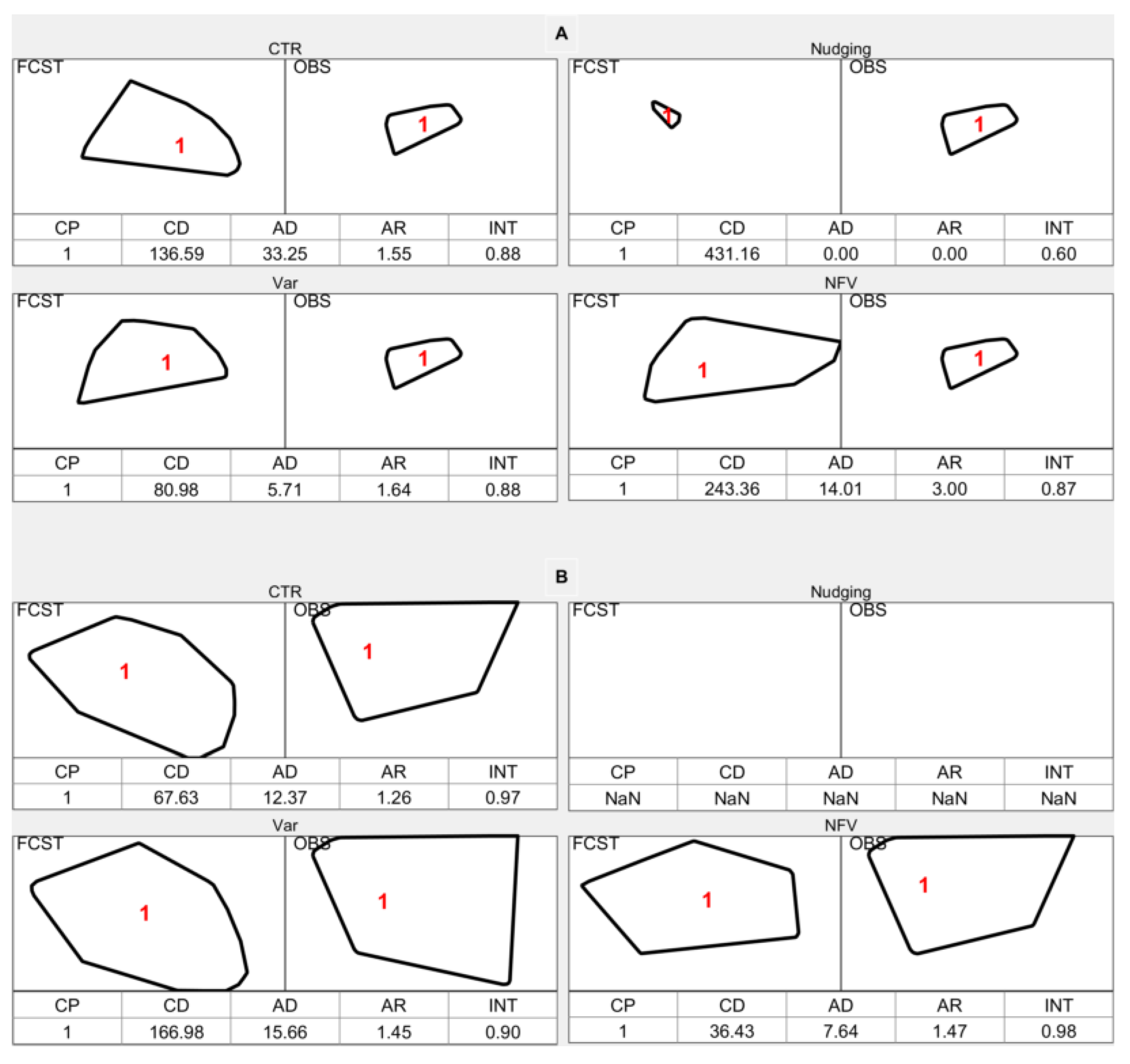
To examine spatial differences in forecast precipitation, multiple geometric attributes of MODE's matched object cluster pairs (CP) are compared (
Figure 11). The 10 UTC SHR event, having the most cases with total interest TI > 0.7 (
Figure 10 Da~Dd), is selected. For SHR (
Figure 11A), Nudging shows the smallest angle difference (AD), the smallest area ratio (AR) and the largest centroid distance (CD), giving the lowest interest (0.6). CTR, Var and NFV yield almost equal interest (0.88); CTR has AR closest to 1, whereas Var has the smallest CD. For rainstorm (
Figure 11B), CTR and NFV share nearly equal interest (0.98), higher than Var (0.90). AR differences among the three are small, but NFV's CD and AD are markedly smaller than those of CTR and Var.
Overall, except for Nudging, all experiments exhibit evident overall false alarms yet missed extremes, with large spreads among nowcasting indicators like SHR, extremes and rainstorm. Nudging keeps the large scale rainfall pattern but with poor skills. Var yields the largest extreme rainfall at 09 UTC, but its spatial pattern departs sharply in time and space. NFV places the forecasted extremes closest to observations and shows the smallest spatiotemporal deviations across all nowcasting metrics, delivering more robust skill. These assimilation dis-/-advantages are likely linked to differing small-scale system development during the period.
5.2.3 Convection
5.2.3.1 Probability density distribution
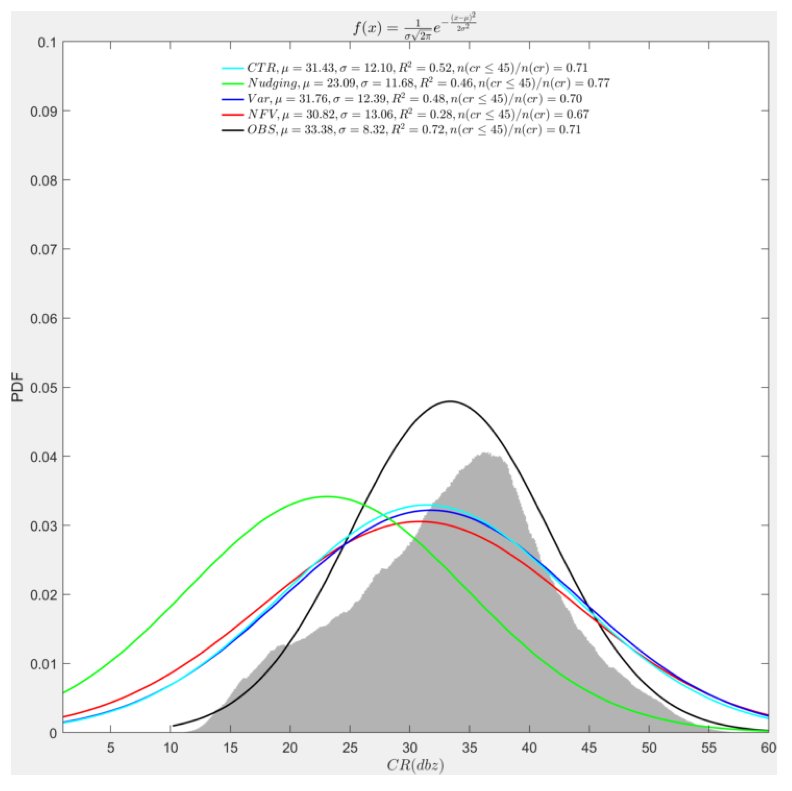
Figure 12 shows differentiated Gaussian distribution fits of CR (about 3.6×10⁷ samples within 1,000 bins), and goodness-of-fit exceeds 0.46 for all data except NFV. Except Nudging, all other PDFs’ centers (
μ) lie around 31~33dBZ, denoting widespread stratiform features. PDFs’ standard deviation (as
σ) is around 12~13dBZ for all data, clearly above the observed 8dBZ, implying broader CR ranges in forecasts. NFV exhibits the lowest weak-CR (<45dBZ) fraction (0.67), signifying the strongest convective development among all datasets.
5.2.3.2 Roebber Skill Scores
Figure 13 compares composite skill for severe convection (CR≥45dBZ). Most points lie in the lower-left of the Roebber diagram; except at 07 and 08 UTC, CSI never exceeds 0.1, indicating low skill. At 07 UTC, Var and NFV are comparable and slightly better than CTR; at 08 UTC, CTR outperforms NFV, while Var shows almost no skill. Thus, severe convection skill of Var is highly uncertain.
5.2.3.3 Severe Convection
Figure 14 compares CR among experiments and observations. Observations show CR ≥ 45 dBZ mainly over Zhengzhou (
Figure 14 Ae~Fe); during 07:00~10:00 UTC, two zebra-striped bands persist, shift slightly southward, shrink markedly, then intensify and move eastward during 11:00~12:00 UTC. In Nudging, the two bands are evident but smaller and displaced (
Figure 14 Ab~Fb). CTR, Var, and NFV overestimate coverage, most pronounced in NFV. During 07:00~09:00 UTC, their patterns are similar, then diverge.
For convective CR, MODE TI is valid (>0.7) for Nudging only during 08:00~10:00 UTC, whereas other experiments exceed 0.7 at all times, indicating good spatial patterns. Var's TI averages around 0.86, slightly better than CTR and NFV.
5.2.3.4 Spatial Object Characteristics
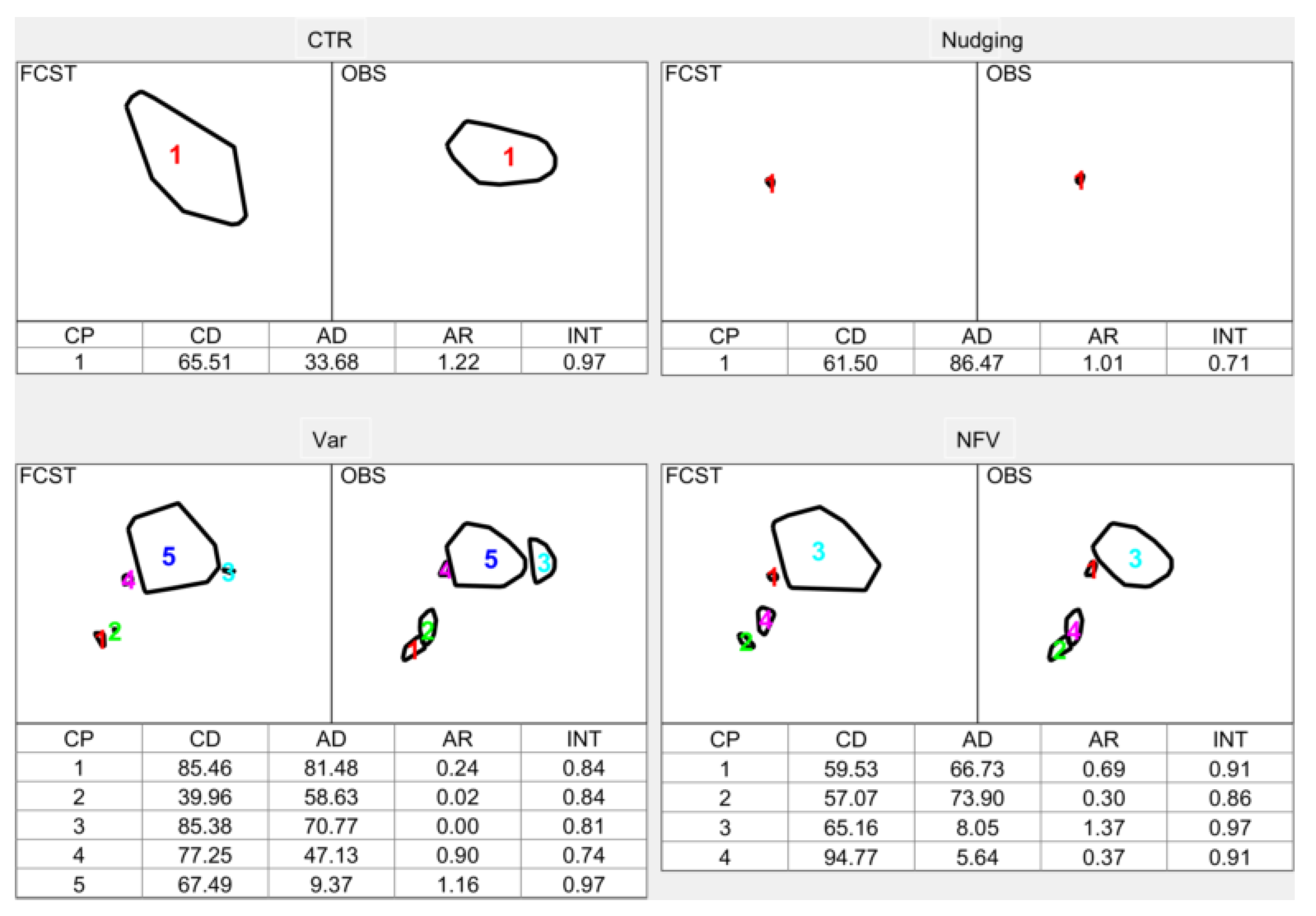
To examine spatial differences in strong echo, geometric attributes of MODE-matched CP are compared at 08 UTC (
Figure 15). The CP counts for Var and NFV exceed others, indicating highly non-uniform shapes and positions. Among the largest clusters, CTR (CP1), Var (CP5) and NFV (CP3) share equal interest (0.97), clearly above Nudging. NFV exhibits the smallest CD and AD, whereas Var's AR is closest to 1.
Overall, except for weaker mean CR in Nudging, all experiments exhibit PDFs consistent with observations. For CR ≥ 45 dBZ, the fraction of all data is uniformly near 0.7, yet skill remains low with evident spatiotemporal disparities. Nudging preserves large-scale convective signatures but clearly misses developing convective zones. Although CTR, Var and NFV share similar TI scores, NFV better maintains convective persistence, whereas CTR and Var shift southward markedly. These are closely correlated with differences in SHR, extreme and rainstorm forecasts.
5.3 Functional Mechanism
5.3.1 Propagation of Forecast Differences
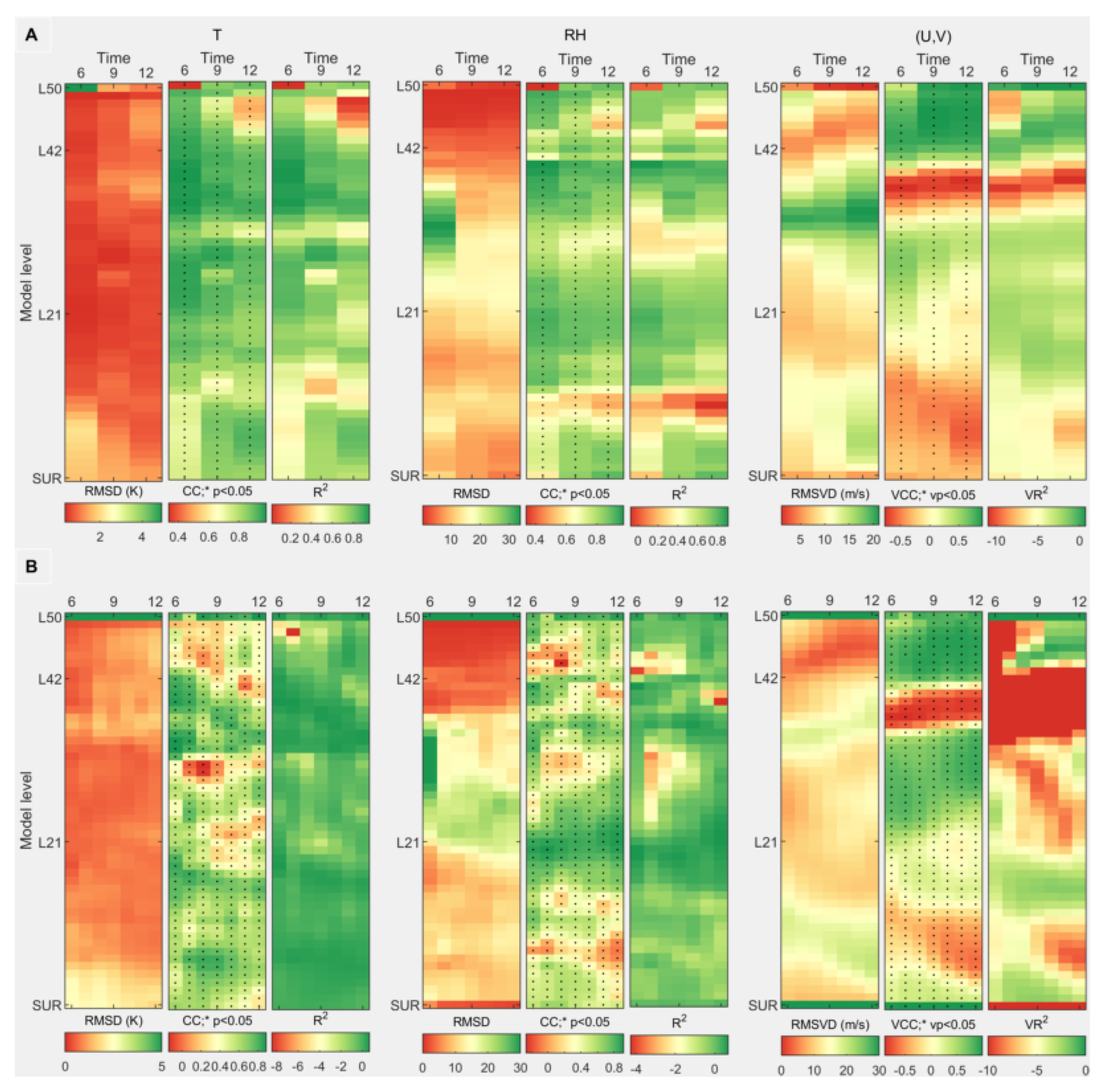
Figure 16 shows spatial RMS differences, correlation coefficients, and goodness-of-fit for T, RH, and vector wind (U, V) between Nudging and Var in D01 and D03. In D01, maximum spatial differences of T occur at L50 of 06 UTC, then weaken and descend to L43. RH peaks at L31 at 06 UTC and weakens afterward. Vector-wind maxima appear at L31 and spread upward to L41. D03 exhibits similar propagation patterns but with notably larger values.
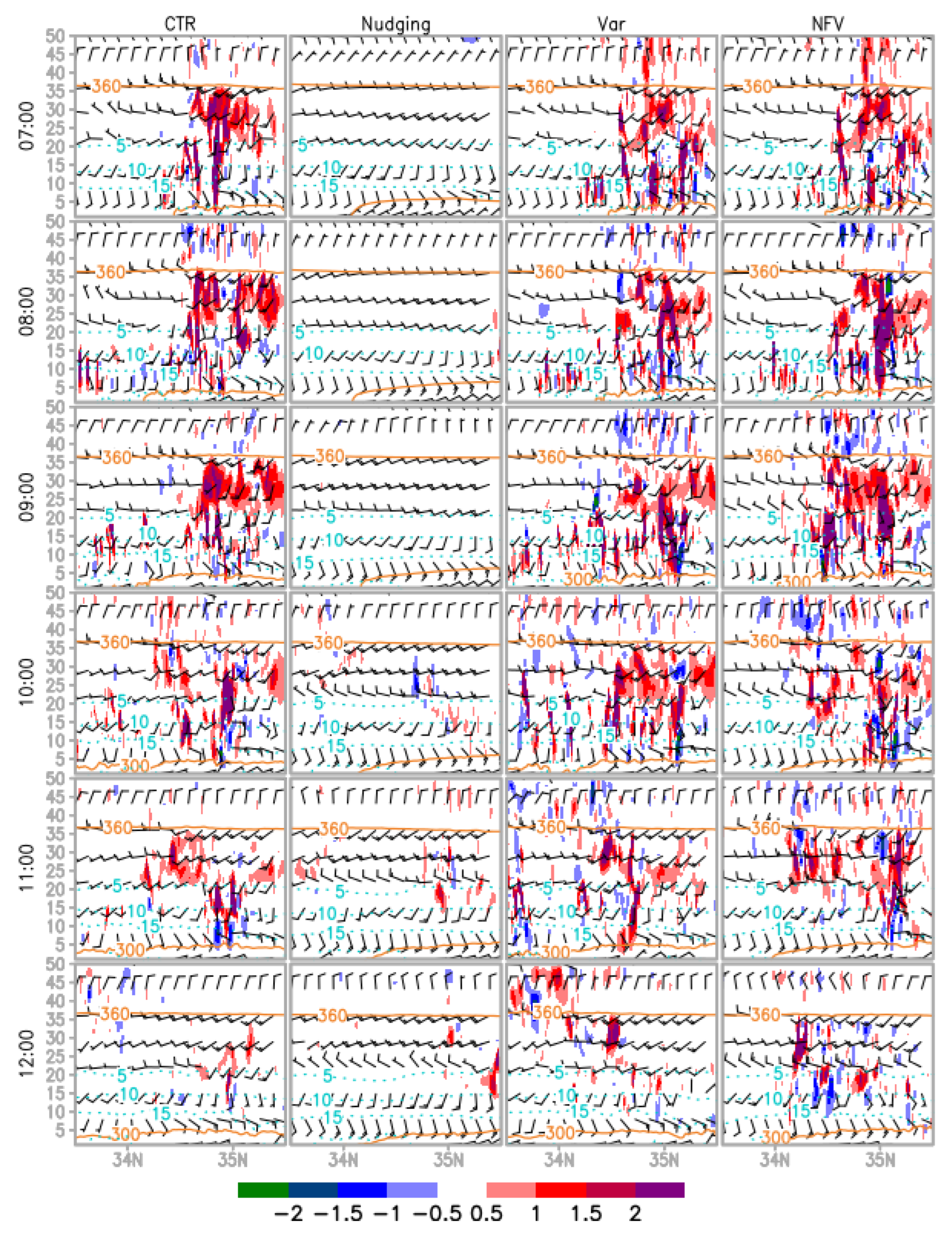
5.3.2 Evolution of Rainfall System
Under RKW maintenance theory, balanced horizontal shear within the cold pool allows deep convection to persist. At 08 UTC, strong divergence near L41 in NFV enhances suction aloft, intensifying convection north of 113.5°E (
Figure 17). The associated northward-tilted vertical vorticity limits southward spreading of the low-level cold pool (
), shifting rainfall northward. This could be linked to enhanced northeasterly increments introduced by Nudging at upper levels. Later, NFV's rainband shifts westward because that weaker low-level vertical shear and convergence over the east produce weaker convection and lower precipitation efficiency.
6. Discussion
Although the NFV method, through simple combination of Nudging and Var, effectively improves forecasts of mid-tropospheric motion, short-duration heavy rain, 6-h rainstorm, and severe convection during the Zhengzhou “7·20” event, it remains limited by observing and modelling capabilities, and the following issues require attention.
1. All schemes exhibit insufficient skill in simulating the widely noted record-breaking 09 UTC rainfall (>200 mm), highlighting limitations of geostationary AMV data for regional application; future enhancement of observations directly linked to precipitation (e.g., Radar data) and optimisation of model physics (e.g., cloud microphysics) is expected to address the poor simulation of extreme precipitation.
2. By combining real-time large-scale Nudging adjustment with high-resolution Var assimilation, NFV enhances simulation of multiple key indicators, yet numerous Nudging and Var parameters crucial to FY4A 3D-winds usage remain; future sensitivity studies of these parameters are essential to further improve geostationary satellite regional applications.
7. Conclusion
This study assimilates FY4A 3D-winds through the developed large-scale nudging-forced high-resolution variational method named NFV; Nudging and Var ablation experiments quantify impacts on assimilation and nowcasting metrics. Main conclusions follow:
1. Large-scale Nudging ingests observations every 3 h and persistently improves linear wind fit versus CTR; high-resolution 3DVar simultaneously improves temperature and wind fits, with both improvements concentrated at the tropopause (400~200 hPa) and Nudging ingesting more observations.
2. For regional high-resolution nowcasting:
1) Upper motion: constrained by observation position accuracy, point-wise improvements from Nudging, Var and NFV are modest; NFV and Nudging TBB evolution agree better with observations than CTR and Var, indicating notable benefit from large-scale adjustment.
2) SHR, extremes and 6-h rainstorm: CTR and Var exhibit larger spatial heterogeneity; NFV shows the highest fractions of both categories. All experiments reproduce the observed north–south rainband, with NFV closest to observations albeit slightly northward. No experiment forecasts the 200 mm 09 UTC peak, yet Var gives the largest extreme (125 mm) and NFV the nearest location. Skill is low for short-duration heavy rain, but NFV outperforms others, especially in 6-h rainstorm spatial pattern.
3) Severe convection: CTR, Var and NFV display stratiform-dominated echoes; NFV has the highest strong-echo fraction, whereas Nudging shows weaker echoes. All three simulate cloud-street patterns close to observations with similar total interest, but NFV slightly over-forecasts. Var strong-echo skill is highly uncertain, while NFV is more stable and accurate, exhibiting the best spatial pattern for the main strong-echo zone.
3.Spatial differences induced by different ingestion methods propagate consistently over D01 and D03: temperature discrepancies descend from model top to tropopause, RH differences descend slightly, and wind-vector differences spread both upward and downward most prominently. FY4A 3D-winds at the tropopause in NFV enhance upper divergence, intensify convection over northern domains and retard southward convection development.
Overall, NFV, integrating FY4A 3D-winds, combines real-time large-scale adjustment with high-resolution assimilation, improves observation usage, enhances upper-level motion forecasts, markedly ameliorates spatial patterns of short-duration heavy rain, 6-h rainstorm and severe convection, and advances short-range prediction of the Zhengzhou “7·20” rainstorm. NFV highlights the benefit of scale-dependent adjustment of geostationary AMVs in regional NWP, yet involves numerous control parameters (e.g., QC thresholds and Nudging scales) whose sensitivities require further investigation to maximize observational efficacy and consolidate these advantages. These findings carry important scientific and practical implications for understanding regional upper systems’ modulation and enhancing local nowcasting capabilityt.
Supplementary Materials
The following supporting information can be downloaded at:
https://www.mdpi.com/article/doi/s1, Figure S1: Impacts on OA Assimilation; Table S1: Main NFV parameter; Equation S1: Method details.
Author Contributions
Conceptualization, Y.Guo and C.S.; methodology, Y.Guo; software, A.S.; validation, Y.Guo, C.S. and A.S.; formal analysis, Y.Guo and D.X.; investigation, Y.Guo and D.X.; resources, A.S. and D.X.; data curation, A.S. and Y.Gao; writing—original draft preparation, Y.Guo; writing—review and editing, Y.Guo, C.S., and A.S.; visualization, Y.Guo; project administration, C.S. and G.N.; funding acquisition, C.S. and G.N. All authors have read and agreed to the published version of the manuscript.
Funding
This research was funded by the Henan Provincial Natural Science Foundation Project (grant number: 242300421367).
Data Availability Statement
The datasets present in this study can be available upon request on the correspondence.
Acknowledgments
We would like to express our gratitude to the CMA Henan Meteorological Bureau, the CMA Meteorological Observation Centre, the CMA National Satellite Meteorological Center, and the CMA Meteorological Development and Planning Institute for their support in carrying out this study. We would like to give our many thanks to those who made efforts to advance this work, and the fellow travelers encountered along the way.
Conflicts of Interest
The authors declare no conflicts of interest.
References
- Bauer, P.; Thorpe, A.; Brunet, G. The quiet revolution of numerical weather prediction. Nature 2015, 525, 47–55. [Google Scholar] [CrossRef]
- Ran, L.; Li, S.; Zhou, Y.; Yang, S.; Ma, S.; Zhou, K.; Shen, D.; Jiao, B.; Li, N. Observational Analysis of the Dynamic, Thermal, and Water Vapor Characteristics of the "7.20" Extreme Rainstorm Event in Henan Province, 2021. Chinese Journal of Atmospheric Sciences 2021, 45, 1366–1383. [Google Scholar] [CrossRef]
- Shi, W.; Li, X.; Zeng, M.; Zhang, B.; Wang, H.; Zhu, K.; Zhuge, X. Multi-model Comparison and High-Resolution Regional Model Forecast Anal-Ysis for the "7 · 20" Zhengzhou Severe Heavy Rain. Transactions of Atmospheric Sciences 2021, 44, 688–702. [Google Scholar] [CrossRef]
- Li, J.; Zheng, J.; Min, M.; Li, B.; Xue, Y.; Ma, Y.; Lin, H.; Ren, S.; Niu, N.; Gao, L.; et al. Progress in Quantitative Applications of Fengyun Meteorological Satellite Observations in Weather Nowcasting(Invited). Acta Optica Sinica 2024, 44, 1800002. [Google Scholar] [CrossRef]
- Wan, X.; Gong, J.; Han, W.; Tan, W. The Evaluation of FY-4A AMVs in GRAPES RAFS. Meteorological Monthly 2019, 45, 458–168. [Google Scholar] [CrossRef]
- Wan, X.; Han, W.; Tian, W.; He, X. The Application of Intensive FY-2G AMVs in GRAPES_RAFS. Plateau Meteorology 2018, 37, 1083–1093. [Google Scholar] [CrossRef]
- Wan, X.; Tian, W.; Han, W.; Wang, R.; Zhang, Q.; Zhang, X. The Evaluation of FY-2E Reprocessed IR AMVs in GRAPES. Meteorological Monthly 2017, 43, 1–10. [Google Scholar] [CrossRef]
- Liang, J.; Chen, K.; Xian, Z. Assessment of FY-2G Atmospheric Motion Vector Data and Assimilating Impacts on Typhoon Forecasts. Earth and Space Science 2021, 8. [Google Scholar] [CrossRef]
- Bormann, N.; Hernandez-Carrascal, A.; Borde, R.; Lutz, H.J.; Otkin, J.A.; Wanzong, S. Atmospheric Motion Vectors from Model Simulations. Part I: Methods and Characterization as Single-Level Estimates of Wind. Journal of Applied Meteorology and Climatology 2014, 53, 47–64. [Google Scholar] [CrossRef]
- Carr, J.; Wu, D.; Daniels, J.; Friberg, M.; Bresky, W.; Madani, H. GEO–GEO Stereo-Tracking of Atmospheric Motion Vectors (AMVs) from the Geostationary Ring. Remote Sensing 2020, 12. [Google Scholar] [CrossRef]
- Santek, D.; Dworak, R.; Nebuda, S.; Wanzong, S.; Borde, R.; Genkova, I.; García-Pereda, J.; Galante Negri, R.; Carranza, M.; Nonaka, K.; et al. 2018 Atmospheric Motion Vector (AMV) Intercomparison Study. Remote Sensing 2019, 11. [Google Scholar] [CrossRef]
- Xu, J.; Lu, F.; Yang, l.; Zhang, X.; Cao, Y.; Zhang, Q.; Shang, J. Image Navigation and Atmospheric Motion Vectors for FY Geosynchronous Meteorological Satellites(Invited). Acta Optica Sinica 2024, 44, 9–23. [Google Scholar] [CrossRef]
- Yang, C.-Y.; Lu, Q.-F.; Wu, X.-B.; Zhang, P. Errors in height assignment for atmospheric motion vectors of FY-2C. Journal of Infrared and Millimeter Waves 2012, 31, 73–79. [Google Scholar] [CrossRef]
- Deb, S.K.; Sankhala, D.K.; Kumar, P.; Kishtawal, C.M. Retrieval and applications of atmospheric motion vectors derived from Indian geostationary satellites INSAT-3D/INSAT-3DR. Theoretical and Applied Climatology 2020, 140, 751–765. [Google Scholar] [CrossRef]
- Chen, Y.; Shen, J.; Fan, S.; Wang, C. A study of the observational error statistics and assimilation applications of the FY-4A satellite atmospheric motion vector. Trans Atmos Sci 2019, 44, 418–427. [Google Scholar] [CrossRef]
- Xie, Y.; Chen, M.; Zhang, S.; Shi, J.; Liu, R. Impacts of FY-4A Atmospheric Motion Vectors on the Henan 7.20 Rainstorm Forecast in 2021. Remote Sensing 2022, 14. [Google Scholar] [CrossRef]
- Li, J.; Menzel, W.P.; Schmit, T.J.; Schmetz, J. Applications of Geostationary Hyperspectral Infrared Sounder Observations: Progress, Challenges, and Future Perspectives. Bulletin of the American Meteorological Society 2022, 103, E2733–E2755. [Google Scholar] [CrossRef]
- Klaes, K.D.; Ackermann, J.; Anderson, C.; Andres, Y.; August, T.; Borde, R.; Bojkov, B.; Butenko, L.; Cacciari, A.; Coppens, D.; et al. The EUMETSAT Polar System: 13+ Successful Years of Global Observations for Operational Weather Prediction and Climate Monitoring. Bulletin of the American Meteorological Society 2021, 102, E1224–E1238. [Google Scholar] [CrossRef]
- Hernandez-Carrascal, A.; Bormann, N. Atmospheric Motion Vectors from Model Simulations. Part II: Interpretation as Spatial and Vertical Averages of Wind and Role of Clouds. Journal of Applied Meteorology and Climatology 2014, 53, 65–82. [Google Scholar] [CrossRef]
- Zhang, Y.; Yao, X.; Di, D.; Li, B.; Zhou, R. Three-Dimensional Wind Field Retrieval by Combining Measurements from Imager and Hyperspectral Infrared Sounder Onboard the Same Geostationary Platform Chinese Journal of Atmospheric Sciences 2023, 47, 1891−1906, doi:10.3878/j.issn.1006-9895.2209.22093. [CrossRef]
- Li, J.; Santek, D.; Li, Z.; Lim, A.; Di, D.; Min, M.; Velden, C.; Menzel, W.P. Tracking Atmospheric Motions for Obtaining Wind Estimates Using Satellite Observations—From 2D to 3D. Bulletin of the American Meteorological Society 2025, 106, E344–E363. [Google Scholar] [CrossRef]
- Rennie, M.P.; Isaksen, L.; Weiler, F.; Kloe, J.d.; Kanitz, T.; Reitebuch, O. The impact of Aeolus wind retrievals on ECMWF global weather forecasts. Quarterly Journal of the Royal Meteorological Society 2021, 147, 3555–3586. [Google Scholar] [CrossRef]
- Okabe, I.; Okamoto, K. Impact of Aeolus horizontal line-of-sight wind observations on tropical cyclone forecasting in a global numerical weather prediction system. Quarterly Journal of the Royal Meteorological Society 2024, 150, 1447–1472. [Google Scholar] [CrossRef]
- Ju, Y.; He, J.; Ma, G.; Huang, J.; Guo, Y.; Liu, G.; Zhang, M.; Gong, J.; Zhang, P. Impact of the Detection Channels Added by Fengyun Satellite MWHS-II at 183 GHz on Global Numerical Weather Prediction. Remote Sensing 2023, 15. [Google Scholar] [CrossRef]
- Wang, H.; Han, W.; Li, J.; Chen, H.; Yin, R. Impact of Assimilation of FY-4A GIIRS Three-Dimensional Horizontal Wind Observations on Typhoon Forecasts. Advances in Atmospheric Sciences 2025, 42, 467–485. [Google Scholar] [CrossRef]
- Wang, Z.; Sui, X.; Zhang, Q.; Yang, L.; Zhao, H.; Tang, M.; Zhan, Y.; Zhang, Z. Derivation of cloud-free-region atmospheric motion vectors from FY-2E thermal infrared imagery. Advances in Atmospheric Sciences 2017, 34, 272–282. [Google Scholar] [CrossRef]
- Eyre, J.R.; Bell, W.; Cotton, J.; English, S.J.; Forsythe, M.; Healy, S.B.; Pavelin, E.G. Assimilation of satellite data in numerical weather prediction. Part II: Recent years. Quarterly Journal of the Royal Meteorological Society 2022, 148, 521–556. [Google Scholar] [CrossRef]
- Eyre, J.R.; English, S.J.; Forsythe, M. Assimilation of satellite data in numerical weather prediction. Part I: The early years. Quarterly Journal of the Royal Meteorological Society 2019, 146, 49–68. [Google Scholar] [CrossRef]
- Ishii, S.; Okamoto, K.; Okamoto, H.; Kimura, T.; Kubota, T.; Imamura, S.; Sakaizawa, D.; Fujihira, K.; Matsumoto, A.; Okabe, I.; et al. Future Space-Based Coherent Doppler Wind Lidar for Global Wind Profile Observation. Cham, 2024; pp. 37-46.
- Gustafsson, N.; Janjić, T.; Schraff, C.; Leuenberger, D.; Weissmann, M.; Reich, H.; Brousseau, P.; Montmerle, T.; Wattrelot, E.; Bučánek, A.; et al. Survey of data assimilation methods for convective-scale numerical weather prediction at operational centres. Quarterly Journal of the Royal Meteorological Society 2018, 144, 1218–1256. [Google Scholar] [CrossRef]
- Lei, L.; Weng, F.; Duan, W.; Chen, Y.; Zhang, L.; Wang, R.; Yang, J.; Qin, X.; Han, W.; Li, J.; et al. Overview and Prospect of Data Assimilation in Numerical Weather Prediction. Journal of Meteorological Research 2025, 39, 559–592. [Google Scholar] [CrossRef]
- Hu, G.; Dance, S.L.; Fowler, A.; Simonin, D.; Waller, J.; Auligne, T.; Healy, S.; Hotta, D.; Löhnert, U.; Miyoshi, T.; et al. On methods for assessment of the value of observations in convection-permitting data assimilation and numerical weather forecasting. Quarterly Journal of the Royal Meteorological Society 2025, 151, e4933. [Google Scholar] [CrossRef]
- Hu, G.; Dance, S.L.; Bannister, R.N.; Chipilski, H.G.; Guillet, O.; Macpherson, B.; Weissmann, M.; Yussouf, N. Progress, challenges, and future steps in data assimilation for convection-permitting numerical weather prediction: Report on the virtual meeting held on 10 and 12 November 2021. Atmospheric Science Letters 2022, 24, e1130. [Google Scholar] [CrossRef]
- Cram, J.M.; Daniels, J.; Bresky, W.; Liu, Y.; Low-Nam, S.; Sheu, R.-S. Use/Impact of NESDIS GOES Wind Data within an Operational Mesoscale RT-FDDA System. In Proceedings of the The 16th Conference on Weather Analysis and Forecasting/13th Conference on Numerical Weather Prediction. 2002. [Google Scholar]
- Rabier, F. Overview of global data assimilation developments in numerical weather-prediction centres. Quarterly Journal of the Royal Meteorological Society 2006, 131, 3215–3233. [Google Scholar] [CrossRef]
- Houtekamer, P.L.; Mitchell, H.L. Ensemble Kalman filtering. Quarterly Journal of the Royal Meteorological Society 2006, 131, 3269–3289. [Google Scholar] [CrossRef]
- Hoke, J.; Anthes, R. The Initialization of Numerical Models by a Dynamic-Initialization Technique. Monthly Weather Review 1976, 104, 1551–1556. [Google Scholar] [CrossRef]
- Otte, T.L.; Seaman, N.L.; Stauffer, D.R. A Heuristic Study on the Importance of Anisotropic Error Distributions in Data Assimilation. Monthly Weather Review 2001, 129, 766–783. [Google Scholar] [CrossRef]
- Christopher, G.K.; Julio, T.B.; Colin, M.Z.; Vincent, E.L.; Katherine, T.C. Do Nudging Tendencies Depend on the Nudging Timescale Chosen in Atmospheric Models? Journal of Advances in Modeling Earth Systems 2022, 14. [Google Scholar] [CrossRef]
- Bullock Jr, O.R.; Foroutan, H.; Gilliam, R.C.; Herwehe, J.A. Adding four-dimensional data assimilation by analysis nudging to the Model for Prediction Across Scales – Atmosphere (version 4.0). Geosci. Model Dev. 2018, 11, 2897–2922. [Google Scholar] [CrossRef] [PubMed]
- Seaman, N.L.; Stauffer, D.R.; Lario-Gibbs, A.M. A Multiscale Four-Dimensional Data Assimilation System Applied in the San Joaquin Valley During SARMAP. Part I: Modeling Design and Basic Performance Characteristics. Journal of Applied Meteorology 1995, 34, 1739–1761. [Google Scholar] [CrossRef]
- Liu, Y.; Warner, T.T.; Bowers, J.F.; Carson, L.P.; Chen, F.; Clough, C.A.; Davis, C.A.; Egeland, C.H.; Halvorson, S.F.; Huck, T.W.; et al. The Operational Mesogamma-Scale Analysis and Forecast System of the U.S. Army Test and Evaluation Command. Part I: Overview of the Modeling System, the Forecast Products, and How the Products Are Used. Journal of Applied Meteorology and Climatology 2008, 47, 1077–1092. [Google Scholar] [CrossRef]
- Wang, H.; Chen, D.; Yin, J.; Xu, D.; Dai, G.; Chen, L. An improvement of convective precipitation nowcasting through lightning data dynamic nudging in a cloud-resolving scale forecasting system. Atmospheric Research 2020, 242, 104994. [Google Scholar] [CrossRef]
- Zhang, X. FY-4B atmospheric motion vector product user guide. Available online: https://img.nsmc.org.cn/PORTAL/NSMC/DATASERVICE/DataFormat/FY4A/FY-4_Product_Cloud_Motion_Vector.pdf (accessed on 11.30).
- Zhang, X.; Xu, J.; Zhang, Q. FY-4 atmospheric motion vector product introduction (Tech. Rep.). Available online: https://img.nsmc.org.cn/PORTAL/NSMC/DATASERVICE/OperatingGuide/FY4B/%E9%A3%8E%E4%BA%91%E5%9B%9B%E5%8F%B7B%E6%98%9F%E4%BA%A7%E5%93%81%E4%BD%BF%E7%94%A8%E8%AF%B4%E6%98%8E%E6%96%87%E6%A1%A3_%E5%A4%A7%E6%B0%94%E8%BF%90%E5%8A%A8%E5%AF%BC%E9%A3%8E.pdf (accessed on 11.30).
- Li, B.; An, n.; Mou, Y. FY-4A AGRI L2 Blackbody Temperature (TBB) Data Format (Dataset). 2022.
- Liu, Z.; Jiang, L.; Shi, C.; Zhang, T.; Zhou, Z.; Liao, J.; Yao, S.; Liu, J.; Wang, M.; Wang, H.; et al. CRA-40/Atmosphere—The First-Generation Chinese Atmospheric Reanalysis (1979–2018): System Description and Performance Evaluation. Journal of Meteorological Research 2023, 37, 1–19. [Google Scholar] [CrossRef]
- Wang, Y.; Yao, S.; Jiang, L.; Liu, Z.; Shi, C.; Hu, K.; Zhang, T.; Zhang, Z.; Liu, J. Collection and Pre-Processing of Satellite Remote-Sensing Data in CRA-40 (CMA's Global Atmospheric ReAnalysis). Advances in Meteorological Science and Technology 2018, 8, 158–163. [Google Scholar] [CrossRef]
- Kain, J.S. The Kain–Fritsch Convective Parameterization: an Update. Journal of Applied Meteorology 2004, 43, 170–181. [Google Scholar] [CrossRef]
- Thompson, G.; Field, P.R.; Rasmussen, R.M.; Hall, W.D. Explicit Forecasts of Winter Precipitation Using an Improved Bulk Microphysics Scheme. Part II: Implementation of a New Snow Parameterization. Monthly Weather Review 2008, 136, 5095–5115. [Google Scholar] [CrossRef]
- Hong, S.-Y.; Noh, Y.; Dudhia, J. A New Vertical Diffusion Package with an Explicit Treatment of Entrainment Processes. Monthly Weather Review 2006, 134, 2318–2341. [Google Scholar] [CrossRef]
- Iacono, M.J.; Delamere, J.S.; Mlawer, E.J.; Shephard, M.W.; Clough, S.A.; Collins, W.D. Radiative Forcing by Long-lived Greenhouse Gases: Calculations with the AER Radiative Transfer Models. Journal of Geophysical Research 2008, 113, D13. [Google Scholar] [CrossRef]
- Jimenez, P.A.; Dudhia, J.; Gonzalez-Rouco, J.F.; Navarro, J.; Montavez, J.P.; Garcia-Bustamante, E. A Revised Scheme for the WRF Surface Layer Formulation. Monthly Weather Review 2011, 140, 898–918. [Google Scholar] [CrossRef]
- Tewari, M.; Chen, F.; Wang, W.; Dudhia, J.; LeMone, M.A.; Mitchell, K.; Ek, M.; Gayno, G.; Wegiel, J.; Cuenca, R.H. Implementation and verification of the unified NOAH land surface model in the WRF model. In Proceedings of the The 20th Conference on Weather Analysis and Forecasting/16th Conference on Numerical Weather Prediction, Seattle, WA, USA, 2004, 12–16 January 2004; pp. 11–15. [Google Scholar]
- Chen, F.; Kusaka, H.; Bornstein, R.; Ching, J.; Grimmond, C.S.B.; Grossman-Clarke, S.; Loridan, T.; Manning, K.W.; Martilli, A.; Miao, S.; et al. The Integrated Wrf/Urban Modelling System: Development, Evaluation, and Applications to Urban Environmental Problems. International Journal of Climatology 2011, 31, 273–288. [Google Scholar] [CrossRef]
- Powers, J.G.; Klemp, J.B.; Skamarock, W.C.; Davis, C.A.; Dudhia, J.; Gill, D.O.; Coen, J.L.; Gochis, D.J.; Ahmadov, R.; Peckham, S.E.; et al. The Weather Research and Forecasting Model Overview, System Efforts, and Future Directions. Bulletin of the American Meteorological Society 2017, 98, 1717–1737. [Google Scholar] [CrossRef]
- Saunders, R.; Hocking, J.; Turner, E.; Rayer, P.; Rundle, D.; Brunel, P.; Vidot, J.; Roquet, P.; Matricardi, M.; Geer, A.; et al. An Update on the RTTOV Fast Radiative Transfer Model (currently at Version 12). Geoscientific Model Development 2018, 11, 2717–2732. [Google Scholar] [CrossRef]
- Roebber, P.J. Visualizing Multiple Measures of Forecast Quality. Weather and Forecasting 2009, 24, 601–608. [Google Scholar] [CrossRef]
- Brown, B.; Jensen, T.; Gotway, J.H.; Bullock, R.; Gilleland, E.; Fowler, T.; Newman, K.; Blank, L.; Burek, T.; Harrold, M.; et al. The Model Evaluation Tools (MET): More Than a Decade of Community-Supported Forecast Verification. Bulletin of the American Meteorological Society 2021, 102, E782–E807. [Google Scholar] [CrossRef]
- Bryan, G.H.; Knievel, J.C.; Parker, M.D. A Multimodel Assessment of RKW Theory's Relevance to Squall-Line Characteristics. Monthly Weather Review 2006, 134, 2772–2792. [Google Scholar] [CrossRef]
- Weisman, M.L.; Rotunno, R. "A Theory for Strong Long-Lived Squall Lines'' Revisited. Journal of the atmospheric sciences 2004, 61, 361–382. [Google Scholar] [CrossRef]
Figure 1.
A. Domains and observations: mesoscale (12-km; red box, D01), small-scale (4-km; gray box, D02), and microscale (1-km; green, D03); FY4A quality-controlled 3D wind vectors at 06:00 UTC (cyan plus), automatic weather stations (AWS, blue dots), and S-band Doppler radar (blue sector, azimuth −45°); terrain (shaded; m). B. FY4A on-orbit schematic and key parameters: field of view (cyan circle), sub-satellite point (yellow dashed cross), satellite-earth distance, and core wavelengths of 3D wind observations. C. On equidistant cylindrical projection: FY4A coverage at 06:00 UTC (cyan ellipse), ch09 AMV winds (vectors; m/s), and D01 location (red box).
Figure 2.
Flowchart of the NFV short-range forecast scheme and its main modules (solid lines). Spin-up denotes a cold-start forecast at −6 h (
). 3DVar denotes observation assimilation over D03 at 0 h (
), with
and
. Nudging denotes successive objective analyses (e.g., OBSGRID's Cressman analysis) with observation and quality-control checks (
QCC) during 0~6 h (
~
). Forcing updating denotes FDDA analysis and forecast during
~
, combining the 3DVar analysis and nudging initialization at
. Note that METGRID, REAL, and OBSGRID details are available at the latest WRF archive as
https://github.com/wrf-model.
Figure 3.
The flowchart of this study. BAK = background. ANA = analysis. FCST = forecast. AMB = analysis minus background. CR = composite reflectivity. SHR = Short-duration heavy rainfall.
Figure 3.
The flowchart of this study. BAK = background. ANA = analysis. FCST = forecast. AMB = analysis minus background. CR = composite reflectivity. SHR = Short-duration heavy rainfall.
Figure 4.
Comparison of observations (OBS) and simulations (SIM) over D03 at 06:00 UTC for 3DVar assimilation. (a)~(c) Linear fits of FY4A OBS (x-axis) versus BAK (blue) and ANA (red) for T, U, V in observation space; RMSE, MAE, CC, and R² are displayed. (d)~(f) Linear fits of OMA (x-axis) and OMB for T, U, V in observation space; gray diagonal indicates assimilation equivalence. (g)~(i) Vertical profiles of domain-averaged AMB for T, U, V in model space; maximum absolute AMB and corresponding layer are marked. (j)~(l) AMB at model layers 21, 35, 41: temperature (shaded) and vector wind; one barb denotes 4 m/s.
Figure 5.
As in
Figure 4, but for OA over D01 at 06:00 UTC.
Figure 5.
As in
Figure 4, but for OA over D01 at 06:00 UTC.
Figure 6.
Linear fits in D03 during 06:00~12:00 UTC between FY4A 3D-winds (x-axis) and forecasts (CTR, Nudging, Var, NFV in black, blue, green, red) for T, U, V, with RMSE, MAE, CC, R² shown.
Figure 6.
Linear fits in D03 during 06:00~12:00 UTC between FY4A 3D-winds (x-axis) and forecasts (CTR, Nudging, Var, NFV in black, blue, green, red) for T, U, V, with RMSE, MAE, CC, R² shown.
Figure 7.
Comparison of TBB retrievals of each experiment in D01 with FY4A ch09 TBB during 06:00~12:00 UTC.
Figure 7.
Comparison of TBB retrievals of each experiment in D01 with FY4A ch09 TBB during 06:00~12:00 UTC.
Figure 8.
Gamma-distribution fits of (left) and (right) for all data over D03; shaded areas show observed scatter.Note: observations in and refer to AWS and CLDAS data, respectively.
Figure 8.
Gamma-distribution fits of (left) and (right) for all data over D03; shaded areas show observed scatter.Note: observations in and refer to AWS and CLDAS data, respectively.
Figure 9.
Roebber diagram comparison of forecast precipitation in D03; left: hourly SHR during 07–12 UTC, right: 6-h rainstorm at 12 UTC. Thick gray marks the 1:1 (POD = SR) no-bias line; thin solid and dashed gray lines indicate CSI and BIAS references.
Figure 9.
Roebber diagram comparison of forecast precipitation in D03; left: hourly SHR during 07–12 UTC, right: 6-h rainstorm at 12 UTC. Thick gray marks the 1:1 (POD = SR) no-bias line; thin solid and dashed gray lines indicate CSI and BIAS references.
Figure 10.
Comprehensive comparison of precipitation forecasts and observations in D03. Panels Aa~Fa, Ab~Fb, Ac~Fc, Ad~Fd, Ae~Fe show
Figure 10.
Comprehensive comparison of precipitation forecasts and observations in D03. Panels Aa~Fa, Ab~Fb, Ac~Fc, Ad~Fd, Ae~Fe show
Figure 11.
Comparison of MODE-matched object cluster pairs between forecast (left, FCST) and observation (right, OBS). A: 10 UTC SHR; B: 6-h rainstorm. CP = cluster pair, CD = centroid distance, AD = angle difference, AR = area ratio, INT = interest.
Figure 11.
Comparison of MODE-matched object cluster pairs between forecast (left, FCST) and observation (right, OBS). A: 10 UTC SHR; B: 6-h rainstorm. CP = cluster pair, CD = centroid distance, AD = angle difference, AR = area ratio, INT = interest.
Figure 12.
As in
Figure 8, but for Gaussian PDF of CR; shaded area shows observed scatter.
Figure 12.
As in
Figure 8, but for Gaussian PDF of CR; shaded area shows observed scatter.
Figure 13.
As in
Figure 9, but for composite skill of CR ≥ 45 dBZ during 07~12 UTC.
Figure 13.
As in
Figure 9, but for composite skill of CR ≥ 45 dBZ during 07~12 UTC.
Figure 14.
As in
Figure 10, but for CR forecasts versus S-band radar CR observations over D03.
Figure 14.
As in
Figure 10, but for CR forecasts versus S-band radar CR observations over D03.
Figure 15.
As in
Figure 11, but for matched-object clusters with CR≥ 45 dBZ at 08 UTC.
Figure 15.
As in
Figure 11, but for matched-object clusters with CR≥ 45 dBZ at 08 UTC.
Figure 16.
Temporal–vertical diffusion of RMSD, CC with significance level p, and R² for T, RH and vector wind (U, V) between Nudging and Var is shown in D01 (A, 3-h) and D03 (B, 1-h).
Figure 16.
Temporal–vertical diffusion of RMSD, CC with significance level p, and R² for T, RH and vector wind (U, V) between Nudging and Var is shown in D01 (A, 3-h) and D03 (B, 1-h).
Figure 17.
Vertical cross-sections along 113.5°E at 07:00~12:00 UTC for all experiments; x-axis denotes latitude, y-axis model level. Variables include vertical velocity (shaded, -2~2 m/s at 0.5 m/s intervals), horizontal wind (vectors, 1 barb represents 4 m/s), equivalent potential temperature (yellow contours, 300 and 360 K), and water-vapor mixing ratio (cyan dotted, 5~15 g/kg at 5 g/kg intervals).
Table 1.
Description of experiments
Table 1.
Description of experiments
| EXPT |
Assimilation*
|
Observation
(elements; error) * |
Background
(domain, scale; error) *
|
Notes |
| CTR |
/ |
/ |
/ |
Control |
| Var |
3DVar |
P, T, U, V;
R |
D03, 1-km; CV5 |
FDDA ablation |
| Nudging |
OA and FDDA |
P, T, U, V;
QCC
|
D01, 12-km; / |
3DVar ablation |
| NFV |
3DVar |
(P, T, U, V); R) |
(D03, 1-km; CV5) |
Reference |
|
Disclaimer/Publisher’s Note: The statements, opinions and data contained in all publications are solely those of the individual author(s) and contributor(s) and not of MDPI and/or the editor(s). MDPI and/or the editor(s) disclaim responsibility for any injury to people or property resulting from any ideas, methods, instructions or products referred to in the content. |
© 2025 by the authors. Licensee MDPI, Basel, Switzerland. This article is an open access article distributed under the terms and conditions of the Creative Commons Attribution (CC BY) license (http://creativecommons.org/licenses/by/4.0/).