

Submitted:
31 March 2026
Posted:
01 April 2026
You are already at the latest version
Abstract
Efficiently and accurately converting floating-point numbers to decimal strings is a critical challenge in numerical computation and data exchange. While existing algorithms like Ryu, Dragonbox, and Schubfach satisfy the Steele-White (SW) principle for accuracy, they often suffer from performance bottlenecks due to branch prediction failures and high-precision multiplication overhead. This paper presents a novel floating-point to string conversion algorithm called "xjb", an optimized variant of the Schubfach algorithm designed to deliver superior performance for IEEE754 single-precision (binary32) and double-precision (binary64) floating-point numbers. By minimizing instruction dependencies, reducing multiplication operations, mitigating branch prediction penalties and by utilizing the simd instruction set, xjb achieves significant performance gains. The algorithm features concise core implementation. Extensive benchmarking across diverse platforms, including AMD R7-7840H and Apple M1, demonstrates that xjb outperforms state-of-the-art algorithms in most scenarios while maintaining full compliance with the SW principle.
Keywords:
floating-point
; printing
; algorithm
; performance
1. Introduction
Floating-point to decimal string conversion is a fundamental operation in computer systems with widespread applications across numerous domains. From scientific computing and financial systems to web services and database management, the ability to efficiently and accurately convert binary floating-point representations into human-readable decimal strings is essential. Despite its apparent simplicity, this conversion problem presents significant challenges in balancing the competing demands of correctness, performance, and output compactness.
1.1. Background and Motivation
In 1990, Steele and White [1,2] published the seminal paper How to Print Floating-Point Numbers Accurately, which established the foundational principles for optimal floating-point printing algorithms, now widely known as the Steele-White (SW) principle. The SW principle comprises four key requirements:
- Information preservation: The printed result must be parseable back to the original floating-point number without loss of precision.
- Minimum length: The output string should be as short as possible while maintaining information preservation.
- Correct rounding: When multiple representations satisfy the first two criteria, the algorithm must correctly round to the nearest value, with ties broken by selecting the even value.
- Left-to-right generation: The output digits should be generated sequentially from the most significant to the least significant digit.
These principles ensure that floating-point numbers have a unique, well-defined decimal representation that is both human-readable and machine-parseable. Algorithms satisfying the SW principle guarantee that the conversion process is reversible and produces the shortest possible output, which is crucial for data exchange, serialization, and user interface display.
Over the past three decades, significant research efforts have been devoted to developing efficient algorithms that satisfy the SW principle. Early approaches, such as the Dragon4 algorithm, provided correct results but suffered from performance limitations due to the use of arbitrary-precision arithmetic. Subsequent innovations introduced various optimizations:
- dtoa.c [3] is an improved version of Dragon4, written by Robert G. Burger and R. Kent Dybvig in 1996. The source code link is https://www.netlib.org/fp/dtoa.c.
- Grisu3 [4] pioneered the use of precomputed powers of ten to avoid expensive arbitrary-precision operations, though it occasionally falls back to slower methods for certain inputs.
- Errol [5] improved upon Grisu3 by reducing the fallback rate through more precise error analysis.
- Schubfach [8] introduced a novel approach based on the concept of "Schubfach" (pigeonhole principle), providing a compact and elegant solution with competitive performance.
- Grisu-Exact [9] eliminated the need for fallbacks entirely while maintaining high performance.
- Dragonbox [10] reduces the number of multiplications by sacrificing more branches.
- yy_double [11] explored alternative computational strategies to minimize the multiplication cost, but there were still a few branches.
- zmij [15] is based on yy_double and has undergone extensive code optimization.
Despite these advances, existing algorithms still face several performance challenges that limit their effectiveness in high-throughput scenarios:
- 1.
- Branch prediction penalties: Many algorithms rely heavily on conditional branches to handle different cases, leading to frequent branch mispredictions on modern pipelined processors.
- 2.
- High-precision multiplication overhead: The conversion process requires high-precision arithmetic operations, particularly multiplications involving large precomputed constants, which can be expensive on standard hardware.
- 3.
- Instruction dependency chains: Sequential dependencies between operations limit instruction-level parallelism and prevent efficient utilization of modern superscalar processors.
- 4.
- Limited SIMD utilization: Most existing algorithms do not exploit vector instruction sets (SIMD) that are now ubiquitous in contemporary processors.
These limitations motivate the need for a new approach that addresses these performance bottlenecks while maintaining full compliance with the SW principle.
1.2. Contributions
This paper presents xjb, a novel floating-point to string conversion algorithm that achieves superior performance through systematic optimization of the underlying computational structure. The xjb algorithm is derived from the Schubfach algorithm and incorporates insights from yy_double and Dragonbox, but introduces several key innovations:
- 1.
- Reduced instruction dependencies: By carefully restructuring the computation, xjb minimizes data dependencies between operations, enabling better instruction-level parallelism and improved pipeline utilization.
- 2.
- Minimized multiplication operations: The algorithm reduces the number of expensive high-precision multiplications required during conversion, significantly decreasing computational overhead.
- 3.
- Mitigated branch prediction penalties: Through branchless programming techniques and careful case analysis, xjb minimizes conditional branches that could lead to prediction failures.
- 4.
- SIMD instruction utilization: The algorithm is designed to leverage SIMD instructions where applicable.
- 5.
- Concise core implementation: Despite its sophisticated optimizations, xjb maintains a compact and readable core implementation, facilitating adoption and maintenance.
The xjb algorithm supports both IEEE 754 single-precision (binary32) and double-precision (binary64) floating-point formats, which are the most widely used floating-point representations in modern computing. For simplicity, this paper uses float to refer to IEEE 754 binary32 and double to refer to IEEE 754 binary64.
1.3. Evaluation Overview
We conducted extensive benchmarking of xjb across diverse hardware platforms, including AMD R7-7840H and Apple M1 processors. Our evaluation demonstrates that xjb outperforms state-of-the-art algorithms in most scenarios while maintaining full compliance with the SW principle. The algorithm exhibits excellent portability and scalability, making it suitable for deployment across a wide range of systems from embedded devices to high-performance servers.
The implementation code for the xjb algorithm and all benchmark tools used in this paper are available at https://github.com/xjb714/xjb.
The remainder of this paper is organized as follows. Section 2 reviews the IEEE 754 floating-point representation and establishes the mathematical foundation for the conversion problem. Section 3 presents the core principles and derivation of the xjb algorithm and describes the implementation details and optimizations. Section 4 presents experimental results comparing xjb against existing algorithms.
1.4. Explanation of Special Symbols in This Article
Provide special explanations for the special symbols used in the formulas of this article.

Table 1.
Explanation of Special Symbols in This Article.
| symbol | brief explanation | example |
|---|---|---|
| % | Integer modulus operation | 2 = 8%3 |
| // | Integer division operation | 1 = 5//3 |
| or | Left or right shift of binary values | 8 = 13 |
| ? : | Similar to the ternary operator in C syntax | a = 1?a:b |
2. IEEE754 Floating-Point Number Representation
This section establishes the mathematical foundation for floating-point number representation and defines the notation used throughout this paper. We focus on the IEEE 754 standard, which is the most widely adopted floating-point arithmetic standard in modern computing systems.
2.1. Scope and Assumptions
For clarity of presentation, we make the following simplifying assumptions:
- We consider only positive floating-point numbers, as negative numbers differ only by a leading minus sign.
- We exclude special values (zero, NaN, and infinity) from our analysis, as these are handled separately in practice.
These assumptions are standard in the literature and do not affect the generality of our algorithm, as the excluded cases can be handled with straightforward special-case logic.
2.2. Binary Representation
Double-precision (binary64): A 64-bit format consisting of:
- 1 sign bit (s): indicates positive () or negative ().
- 11 exponent bits (e): biased exponent in the range .
- 52 fraction bits (f): significand fraction in the range .
Single-precision (binary32): A 32-bit format consisting of:
- 1 sign bit (s): indicates positive () or negative ().
- 8 exponent bits (e): biased exponent in the range .
- 23 fraction bits (f): significand fraction in the range .
2.3. Classification of Floating-Point Numbers
We classify floating-point numbers into three categories based on their exponent and fraction fields:
- 1.
- Subnormal numbers ( and ): These represent very small values close to zero, where the implicit leading bit of the significand is 0 instead of 1.
- 2.
- Normal numbers ( and ): The standard case where the implicit leading bit of the significand is 1.
- 3.
- Irregular numbers ( and ): Numbers with zero fraction field, representing powers of two.
We use the term regular to refer to both subnormal and normal numbers (i.e., all cases where ).
2.4. Value Representation
The real value v of a positive floating-point number can be expressed in the unified form , where c is the integer significand and q is the exponent. The general formula covering all cases is:
For each category, the values decompose as follows:
Subnormal numbers ():
Irregular numbers (, ):
Normal numbers (, ):
2.5. Rounding Intervals
A critical concept for accurate floating-point printing is the rounding interval , which defines the range of real numbers that round to the given floating-point value v when parsed. The rounding interval is bounded by:
The rounding radius for regular floating-point numbers is . The distinction between closed and open intervals at the boundaries depends on the parity of the significand, ensuring correct rounding according to the round-to-even rule specified in the IEEE 754 standard. Any decimal number within will parse back to the original floating-point value v, which is essential for ensuring the information preservation property of the SW principle.
3. Principle of Algorithm
This section presents the algorithmic principles and mathematical foundation of the xjb floating-point to string conversion algorithm. We first introduce the overall architecture and design goals, followed by the mathematical formulation of the conversion problem.
3.1. Design Overview
This paper focuses on converting float (single-precision) and double (double-precision) floating-point numbers to decimal strings. The conversion process consists of two stages:
- 1.
- Float-to-Decimal Conversion: Converting binary floating-point values to decimal significand-exponent pairs .
- 2.
- Decimal-to-String Conversion: Formatting into human-readable strings.
We focus primarily on the first stage, as it is the computationally intensive component that benefits most from our optimizations.
The xjb algorithm is designed with four key performance objectives:
- Minimize branch mispredictions through unlikely branches and branchless techniques
- Reduce expensive high-precision multiplication operations
- Optimize instruction dependencies to enable better parallelism
- Maintain core implementation simplicity and readability
3.2. Mathematical Foundation
Before presenting the algorithm details, we establish the mathematical framework for the float-to-decimal conversion problem.
Recall from Section 2 that any floating-point value v can be expressed in the form , where c is the integer significand and q is the exponent. Our goal is to find the optimal decimal representation that satisfies the SW principle.
As established in Section 2, regular floating-point numbers (which include all normal and subnormal numbers with non-zero fraction fields) account for the vast majority of possible floating-point values. For the purposes of algorithm derivation, we focus primarily on regular numbers, as special cases can be handled with minimal additional logic.
The valid ranges for the significand c and exponent q for regular floating-point numbers are:
For irregular floating-point numbers (powers of two), the ranges are:
For subnormal numbers:
The conversion problem can now be formally stated as: given a floating-point value , find the optimal decimal representation such that:
where is the rounding interval of v as defined in Section 2.
For example, consider the IEEE 754 binary64 floating-point number representing 1.3. Its actual value is 1.3000000000000000444089209850062616169452667236328125, with hexadecimal representation 3ff4cccccccccccd. The optimal decimal representation satisfying the SW principle is simply 1.3. Similarly, for the binary32 representation of 1.3, with actual value 1.2999999523162841796875 and hexadecimal representation 3fa66666, the optimal representation is also 1.3.
3.3. Review of the Schubfach Algorithm and Our Derivation
This section reviews the Schubfach algorithm and presents our derivation of an optimized variant. We begin by establishing the mathematical foundation for determining the optimal decimal representation.
3.3.1. Candidate Values for the Significand d
The Schubfach algorithm identifies four candidate values for the decimal significand d:
The exponent k is computed as:
For efficient computation on modern processors, Equation (11) can be implemented using integer arithmetic:
3.3.2. Decomposition into Integer and Fractional Parts
Let denote the integer part and the fractional part, where . Substituting into Equation (10):
Since , the candidates simplify to:
Based on the Schubfach algorithm and the SW principle, if the value or falls within the range , it is selected as the optimal solution d. In cases where neither nor lies within , the optimal solution d is determined as either or in accordance with the rules of correct rounding. We decompose d as , where and . The problem thus reduces to determining the appropriate value of .
3.3.3. Selection Criteria for
The selection of depends on the relationship between the rounding interval and the candidate values. Recall that the rounding interval for a regular floating-point number is , where represents the half-unit in the last place (ulp) of v.
-
Case (i.e., ): This case applies when is the closest representable decimal to v within the rounding interval. The condition is derived as follows:The lower bound of the rounding interval must be less than :When equality holds (), we apply the round-to-even rule, requiring c to be even:
-
Case (i.e., ): This case applies when is the closest representable decimal to v. The condition is derived similarly:The upper bound of the rounding interval must be greater than :When equality holds (), we again apply round-to-even:
-
Case : When neither boundary condition applies, the optimal value lies between and . We determine by rounding to the nearest integer:
- –
- If the fractional part :
- –
- If the fractional part :
- –
- If the fractional part : apply round-to-even
For irregular floating-point numbers (powers of two), additional verification is required to ensure the selected value lies within the rounding interval , as the interval boundaries differ for these special cases.
3.3.4. Algorithm Overview
Algorithm 1 summarizes our optimized variant of the Schubfach algorithm (xjb32 for float, xjb64 for double). Given inputs c and q, the algorithm returns d and k such that satisfies the SW principle. The computation of k follows Equation (12); the remainder of this section focuses on efficient computation of d.
The subsequent sections detail:
- 1.
- Lookup table precomputation
- 2.
- Efficient computation of m
- 3.
- Fast boundary condition testing for
- 4.
- Efficient computation of and rounding
- 5.
- Handling of irregular floating-point numbers
- 6.
- implementation of pseudocode
The following will discuss the above content in detail from Section 3.4 to Section 3.9.
| Algorithm 1:The xjb Algorithm for Float-to-Decimal Conversion |
|
3.4. Lookup Table Precomputation
The algorithm in this paper employs a lookup table to store pre-computed values of for different ranges of q: for float and for double. These lookup tables use extended precision: 64-bit for float and 128-bit for double. The reference implementation is available in gen.py.
3.4.1. Fundamental Calculation
Let B denote the bit length of each entry in the lookup table, with for float and for double. For any integer (representing a power of 10), we aim to represent in the form , where and is a real number. This gives:
Taking the logarithm base 2 of both sides, we get:
Solving for f gives:
The lookup table entries are computed using upward rounding:
Notably, becomes an integer for certain ranges of : for float and for double.
3.4.2. Detailed Calculation Process
The detailed calculation process is as follows:
-
FloatThe range of is calculated to be [-32, 44] through the q value range in Equation (6), so the lookup table contains representation values from 10 to the power of -32 to 10 to the power of 44. The calculation process is as follows:When , the lookup table variable indicates that the values and are equal. In other cases, the relative error is less than . Expressed as:
-
DoubleThe range of is calculated to be [-293, 323] through the q value range in Equation (6), so the lookup table contains representation values from 10 to the power of -293 to 10 to the power of 323. The calculation process is as follows:When , the lookup table variable indicates that the values and are equal. In other cases, the relative error is less than . Expressed as:
Let denote the error for float lookup table entries, for double entries, and r for both. In Algorithm (1), we retrieve from the lookup table. The lookup table provides exact values when q falls within specific ranges:
For q outside these ranges, the lookup table entries have bounded relative errors:
3.4.3. Storage Requirements
The float lookup table requires 616 bytes of storage, calculated as bytes (77 entries × 8 bytes each). The double lookup table requires 9872 bytes, calculated as bytes (617 entries × 16 bytes each).
3.4.4. Implementation Notes
3.5. Efficient Computation of m
This section presents an efficient method for calculating m in Algorithm (1), which is defined as .
3.5.1. Relevant Theorems
We start with some theorems from the Dragonbox algorithm paper:
Let n, P, and Q be positive integers where P and Q are coprime, , , and . Let be the best rational approximation of with and be the best rational approximation with .
If does not divide Q evenly:
Suppose the following holds:
Then:
Thus, the range of is:
The range of the fractional part of is:
Here, the fractional part is minimized when and maximized when .
3.5.2. Best Rational Approximation Function
We define the best rational approximation function (implemented in test1.py):
This function calculates the best rational approximation with denominator not exceeding C using the Farey sequence median theorem. and are adjacent terms in the C-th order Farey sequence . Therefore, we can calculate Equation (34) very quickly.
3.5.3. Key Proof
In Algorithm (1), we need to compute . We aim to prove:
Where r is the lookup table error defined in Equations (25) and (27). When condition (28) is met, , and the equation holds trivially. For :
Calculate the range of and we get:
When q is not 0, Equation (38) exists:
When q is 0, , so the final conclusion is:
Because there is:
Therefore:
Suppose:
Then there are:
3.5.4. Bit Width Calculation
Define maximum values for c:
Let C denote either or depending on the precision.
For , compute and for each q using and find the minimum such that:
For :
Thus:
Similarly, find the minimum such that:
3.5.5. Results
Thus:
This result confirms that m can be calculated efficiently using the lookup table values, even with their inherent errors. Once m is determined, can be computed quickly.
3.6. Fast Boundary Condition Testing for and
In Algorithm 1, the conditions for determining and appear on lines 31 and 34, respectively. This section introduces an optimized method to quickly test these boundary conditions using equivalent mathematical formulations.
3.6.1. Equivalent Conditions for Boundary Testing
We start by deriving equivalent mathematical conditions for testing and .
Case 1: Testing
When , this is equivalent to:
Case 2: Testing
When , this is equivalent to:
3.6.2. Integer Testing Analysis
To further analyze these conditions, we start with the range of from Equation (40):
Analysis for
For the case, we can derive:
This implies that when is an integer, it must equal .
Analysis for
Similarly, for the case:
This implies that when is an integer, it must equal .
3.6.3. Key Insight: Integer Divisibility Test
The key insight is that testing for or is equivalent to checking whether is an integer. This can be rewritten as:
We analyze different ranges of q to simplify this condition:
-
Case : From , we get . The expression simplifies to checking if is divisible by . Since 2 and 5 are coprime, this reduces to checking if is divisible by :Let t be a positive integer such that . Since is odd, t must also be odd. Considering the ranges of c for float and double:This gives us the range for t:The maximum values of k where t can be at least one odd integer are:
- Case : The denominator is even, while the numerator is odd, so no solution exists.
- Case : The denominator is even, while the numerator is odd, so no solution exists.
3.6.4. Summary of Boundary Conditions
In summary, the situations when is an integer are as follows:
The range of is:
3.6.5. Efficient Implementation
We can further simplify the testing conditions using bitwise operations. For :
When , the following conclusions can be drawn:
The discussion on whether in Equation (65) holds true, that is, whether in Equation (65) is an integer, or equivalent to discussing whether the following values are integers when Equation (62) holds true (the same applies to double) :
Suppose c can divide evenly (where t is a temporary integer variable):
Therefore, when Equation (67) was established, there were:
Expression (68) cannot divide evenly, which contradicts Equation (62), so c cannot divide evenly. Therefore, for float, and are not integers; For double, and are not integers, that is:
Therefore, the conclusion (65) is correct. Discuss the necessary and sufficient conditions for whether is . The same applies to double, expressed as:
Similarly, the necessary and sufficient conditions for whether is . The same applies to double, expressed as:
The sufficient conditions of Equations (70) and (71) are obviously established. Introduce the proof that Equation (70) holds. For float, only the necessary conditions need to be discussed, that is, whether must hold true when holds, or equivalent to must hold true when . The following is proved by proof by contradiction.
Assume that holds when . Then there is:
As is known from Equation (55), there is:
Suppose the decimal part of is represented as , thus we have:
Substitute expression (74) into expression (72), and we get:
Similarly, it can be known that the double range is the range of . Therefore, there is:
When , it is known from Equation (52) that is not an integer. Therefore, there is:
It is only necessary to prove that Equation (76) does not hold. Discuss the range of the decimal part when is not an integer. According to Equation (57), there are:
The maximum value of is:
Discuss based on the denominator range in Equation (78).
-
When , is the expression (79), the following holds true:Therefore, when , Equation (76) does not hold true.
-
Call function (35) to calculate the approximation results and of all possible upper and lower limit rational numbers:Therefore, for , the following conclusion can be drawn from formula (34).Therefore, when , Equation (76) does not hold true.
In summary, when , Equation (76) does not hold true, that is, must hold true. Therefore, when holds, must hold true. Therefore, Equation (70) holds.
Similarly, it can be proved that when holds, must hold true. The same applies to double. Similarly, by proof of contradiction, for float, it is assumed that when holds, holds. That is:
As is known from Equation (56), there is:
Suppose the decimal part of is represented as , thus we have:
Similarly, it can be known that the double range is the range of . Therefore, there is:
When , it is known from Equation (53) that is not an integer. Therefore, there is:
It is only necessary to prove that Equation (89) does not hold. Discuss the range of the decimal part when is not an integer. According to Equation (57), there are:
The maximum value of is:
Discuss based on the denominator range in Equation (91).
-
When , is the expression (92), the following holds true:Therefore, when , Equation (89) does not hold true.
-
Call function (35) to calculate the approximation results and of all possible upper and lower limit rational numbers:Therefore, for , the following conclusion can be drawn from formula (34).Therefore, when , Equation (89) does not hold true.
In summary, when , Equation (89) does not hold true, that is, must hold true. Therefore, when holds, must hold true. The same is true for double.Therefore, Equation (71) holds.
The following conclusions hold:
There are:
It has been proven earlier that m can be accurately calculated. Then, when (99) holds true, the values and on the right side of Equations (64) and (65) can be accurately calculated.
From Equation (57), we have:
When conditions (62) and (63) are met, and are integers. Under the condition of meeting condition (62), the decimal part of expression (102) is represented as:
It is only necessary to prove that the increase in the value on the right side of the expression compared to the value on the left side plus the decimal part of the value on the left side is less than 1 for Equation (99) to hold true. That is:
By exhaustionally calculating the maximum possible c value under each q and substituting it into Equation (104), it holds. The calculation result is in test2.py. The calculation results show that for the float range and the double range, Equation (104) always holds true. Therefore, Equation (99) holds true, and thus the values of and on the right side of Equations (64) and (65) can be accurately calculated. The values of and on the left side of Equations (64) and (65) can be calculated through lookup tables.
The code file for verifying the validity of Equation (105) is test4.py. Therefore, when conditions (62) and (63) are met, the values of both sides of Equations (64) and (65) can be accurately calculated.
Discuss the relationship between the following two values within all ranges of floating-point numbers:
When , it is obvious that the two values in expression (106) are equal. When , or equivalent to , has:
Therefore, there is:
Because there is:
Suppose:
Therefore, the following conclusion can be drawn: when condition (62) is met, from Equation (99), we have:
Within the range of floating-point numbers, there exists:
To simplify the expression, is used to indicate whether c is an even number:
When or , is the boundary condition for , and is the boundary condition for . Whether is 0 or 10 is determined based on whether c is an even number.Therefore, the following exists:
Therefore, when or , we can use the condition (116) to determine whether or .
When or , We can also use the above condition (116) to determine whether or . When or , we can also use the above condition (116) to determine whether or . There are a total of four situations.The proof is as follows:
(1)When , there must exist , and there is:
Therefore, the following exists:
Suppose there are two real numbers a and b, and the following relationship must exist:
When and or and , the following exists:
From Equation (118), we have:
Therefore, there is:
Therefore, when , the condition (116) can be used to determine that .
(2)When , there must exist , and there is:
Therefore, the following exists:
When and or and , from Equation (119), the following exists:
From Equation (124), we have:
Therefore, there is:
Therefore, when , the condition (116) can be used to determine that .
(3)When , there must exist , and there is:
Therefore, the following exists:
Suppose there are two real numbers a and b, and the following relationship must exist:
When and or and , the following exists:
From Equation (129), we have:
Therefore, there is:
Therefore, when , the condition (116) can be used to determine that .
(4)When , there must exist , and there is:
Therefore, the following exists:
When and or and , from Equation (130), the following exists:
From Equation (135), we have:
Therefore, there is:
Therefore, when , the condition (116) can be used to determine that .
From the above proof, it can be seen that when condition (62) is met, the condition (116) can be used to determine whether or when or . When or , the condition (116) can be used to determine whether or . When or , the condition (116) can be used to determine whether or .
The proof process of this section is completed. In the code implementation, the two judgment conditions can be quickly calculated using addition and subtraction shift operations, and can be compiled by the compiler into cmov instructions, thereby reducing the impact of branch prediction failure on performance.
Ultimately, we reached the following conclusion: can quickly determine whether equals 0 or 10 by using the following method.
3.7. Efficient Computation of and Rounding
Determine whether is or based on the decimal part of . There are two cases: the decimal part of is 0.5 and it is not 0.5.
3.7.1.
When the decimal part of is 0.5, there must be:
So is an odd number. Then the following expression is odd:
According to the range of q, there are:
According to the range of q, the following situations are discussed:
-
When , it can be concluded that , the numerator is even and the denominator is odd, which does not meet the condition.
-
When , it can be concluded that is even, which does not meet the condition.
-
is an odd number. c is an odd multiple of . So:Therefore, when q meets the above conditions, c must be an odd multiple of to meet the condition. Therefore, when the following conditions are met, expression (141) is an odd number:The following equation holds:Since , is multiple of 5 and is an odd number. Since and are both odd numbers, is an even number, is multiple of 5 and is an odd number. Therefore, there is:The result of is an even number between and . Therefore:
3.7.2.
When the decimal part of is not 0.5, round to the nearest integer value based on the decimal part of . Therefore, there is:
Since , it is only necessary to accurately calculate the value of . And, there is:
Suppose there are:
Suppose the decimal part of is .
When , the range of the decimal part must include:
When , the range of the decimal part must include(the test file is test5.py):
Therefore, the range of satisfies Equation (153). In the code implementation, for float, only the high 36 bits of are retained, and for double, only the high 70 bits of are retained. Suppose the discarded part of a float is represented as , and similarly, the discarded part of a double is represented as . Therefore, there is:
Calculate the boundary conditions of the following expression:
Therefore, there is:
Therefore, there is:
In fact, in the above proof process, for float, may exist, but the code implementation has passed the exhaustive test, so this not-so-perfect proof process can be ignored. Therefore, the calculation of d can be simplified as follows:
For the float range, ; for the double range, .
3.7.3. Efficient Implementation of for Double
For double, quickly determine that in Equation (148).
When ,. Therefore, the following condition can be used to quickly determine whether :
When ,Calculate the range of the decimal part of the following expression:
Calculate the two boundary cases of that are closest to 1:
Then there are:
Therefore, the following condition can be used to quickly determine whether :
In summary, for double, the following condition can be used to quickly determine whether :
3.7.4. Efficient Calculation of for Double
In the double range, introduce another faster way to calculate :
The proof of Equation (166) is as follows:
when , ;
when , Equation (166) can be equivalent to the following:
According to the range, is represented as:
Therefore,when , we need to prove that the following equation holds:
From the range of n, there is:
Because the following conditions exist:
Therefore, the following relationship can be concluded:
Discuss the range of values of x when the following conditions are met.
Therefore, the following conclusions can be drawn:
Suppose . Through the exhaustive method, all floating-point numbers that do not meet the following conditions can be obtained.
All floating-point numbers that do not meet condition (176) are as follows (in hexadecimal) :
Through the exhaustive method, all floating-point numbers that do not meet the following conditions can be obtained.
All floating-point numbers that do not meet condition (178) are as follows (in hexadecimal) :
There are:
When the floating-point number is not within the above range (177) and (179), the condition (175) is satisfied. We have tested all floating-point numbers within the above-mentioned range (177) and (179), and the algorithm implementation code has output the correct result, that is, it satisfies the SW principle. The test process file is test8.py.
3.8. Irregular Number
Due to the limited and small number of irregular floating-point numbers, there are a total of 2046 double floating-point numbers and 254 float floating-point numbers. The correctness of the algorithm code in this paper can be proved by the exhaustive method. Therefore, it is not introduced in this article. For the specific implementation process, please refer to the source code.
3.9. Implementation of Pseudocode
This subsection details the pseudocode implementation for converting regular floating-point numbers to decimal representation. The handling of subnormal (irregular) floating-point numbers is omitted here due to space constraints; interested readers may refer to the source code for the complete implementation.
3.9.1. Single-Precision Floating-Point Numbers
Algorithm 181 outlines the procedure for computing d and k for single-precision floating-point numbers.
Since c contains at most 23 significant bits and has 64 significant bits, their product contains at most 87 significant bits. Given that the range of h is , the value does not overflow, preserving all bits of c. When , is computed using Equation (24). From Equation (25), we derive:
From Equation (51):
When , we have ; when , we have . Therefore:
The upper 28 bits of represent m, while the lower 36 bits represent :
Consequently:
Let indicate whether , equivalently whether the last digit of d is zero:
The following equations hold:
Therefore:
Thus, the condition for is:
Adding serves as a rounding operation. When , Equation (148) requires checking whether . The derivation of involves careful handling of edge cases; the correctness of this computation has been verified through exhaustive testing.
3.9.2. Double-Precision Floating-Point Numbers
Algorithm 194 presents the corresponding procedure for double-precision floating-point numbers. is computed using Equation (26), satisfying:
From Equation (51):
Given and c having at most 53 significant bits, does not overflow, ensuring accurate computation of . By definition, . From Equation (105):
The value of is first computed using Equation (166), then adjusted if the conditions for or are met:
An equivalent formulation is:
In the C/C++ implementation, the only branch occurs when computing c and q for subnormal floating-point numbers (marked as ). The conversion of normal floating-point numbers is branch-free, eliminating branch misprediction penalties. As shown in Algorithms 181 and 194, the core algorithm is remarkably concise. Irregular numbers are handled in a separate branch—a worthwhile trade-off given their rarity.
3.10. Decimal to String Conversion
The floating-point number printing algorithm consists of two main phases. While the first phase, which computes the decimal digits d and exponent k, has been discussed in previous sections, this section focuses on the second phase: converting the computed decimal representation into a string.
Floating-point numbers are typically printed in two formats: fixed-point notation and scientific notation. Table (Table 3) illustrates examples of both formats.
Having computed d and k, we now convert the floating-point number to a string based on these values. According to the Schubfach algorithm, d may contain trailing zeros, meaning could be zero. In order to reduce instruction dependencies. We decompose d into two parts: and . Let indicate whether equals 10, and represent the cases where is either 0 or 10. The following relationships hold:
By calculating the approximate range of m, we obtain:
Based on the range of c, we derive:
Let denote the number of decimal digits in x. For :
We define . For example, . Consequently:
Since , we have . Let denote the number of trailing zeros in the decimal representation of x; for example, . The number of significant digits equals . When , , thus and . Therefore:
For normal floating-point numbers, can be computed as:
where denotes the Iverson bracket, which evaluates to 1 if predicate P is true and 0 otherwise.
Computing the ASCII representation of d reduces to computing the ASCII codes of and . From the above, we have:
These bounds allow efficient computation of the ASCII code for using CPU SIMD instruction sets.
Scalar Implementation
We first present a scalar method that does not rely on SIMD instructions.
Let and be a function that computes the ASCII representation of x. Algorithm (2) describes this process. This version is an optimized version of the itoa algorithm written by Paul Khuong [18].
| Algorithm 2:Convert an 8-digit decimal number to ASCII: dec_to_ascii8(x) |
|
The function simultaneously computes as the return value . Example: X = 12345600, Y="12345600", tz=2.
| Algorithm 3:Convert a 16-digit decimal number to ASCII: dec_to_ascii16(x) |
|
For , let compute the ASCII representation of x. Algorithm (3) describes this process. Example: X = 123456001234500, Y="1234560012345600", tz=2.
Handling Undefined Behavior
Since is undefined behavior in C, special handling is required. For single-precision floating-point numbers, when (the six smallest subnormal numbers), , avoiding the undefined case. For double-precision numbers, only occurs for (the smallest subnormal number). In our implementation, we handle this special case separately at the function entry.
SIMD Implementation
The SIMD implementations of and follow the same principles as the scalar version. For ARM64 architecture, we use the NEON instruction set; for x64 architecture, we support three variants: AVX512, SSE4.1, and SSE2. Table (Table 4) summarizes these implementations.
Using the methods above, we compute the ASCII representation of and the number of significant digits. Printing d is equivalent to printing and . Based on , we determine which buffer contents to retain. In our implementation, we adopt different formats for floating-point numbers in different ranges to enhance readability, as shown in Table (Table 5).
In scientific notation, the result includes an exponent. For example, in “1.2e-02”, “e-02” represents the exponent. Converting to standard decimal scientific notation yields:
Since , the exponent is determined by . Let . Then:
For single-precision floating-point numbers, fixed-point notation is used when . For double-precision numbers, fixed-point notation is used when .
The floating-point number printing algorithm proposed in this paper is illustrated as Algorithm 4. The key distinction between our algorithm and others is the use of SIMD instruction sets for converting to ASCII values. For single-precision numbers, we use ; for double-precision, we use . The detailed implementation is available in the source code.
| Algorithm 4:Floating-point number printing algorithm |
|
In our C implementation, all branches are designed as unlikely branches to minimize the impact of branch prediction failures. By transforming the computation of d into computing and , we reduce instruction dependencies and enhance instruction-level parallelism. Unlike other algorithms that compute the exact value of d before printing, we avoid computing d directly and instead quickly compute .
3.11. Summary
This chapter explains how to quickly calculate d and k, as well as the printing optimization. Since , the process of calculating d is transformed into calculating m and .
- Section 3.5 introduces the method for quickly calculating m.
- Section 3.6 and Section 3.7 introduce the methods for quickly calculating .
- Section 3.9 provides a detailed description of the pseudo-code implementation.
- Section 3.10 discusses print optimization.
Table 6.
All algorithms in the benchmark test.
| algorithm | float | double | description |
|---|---|---|---|
| Schubfach | Schubfach32 | Schubfach64 | author:Raffaello Giulietti,https://github.com/c4f7fcce9cb06515/Schubfach. |
| Schubfach_xjb | Schubfach32_xjb | Schubfach64_xjb | It is improved by Schubfach and has the same output result. |
| Ryu | Ryu32 | Ryu64 | author:Ulf Adams,https://github.com/ulfjack/ryu. |
| Dragonbox | Dragonbox32 | Dragonbox64 | author:Junekey Jeon,https://github.com/jk-jeon/Dragonbox. |
| fmt [22] | fmt32 | fmt64 | author:Victor Zverovich,https://github.com/fmtlib/fmt version:12.1.0 |
| yy_double | - | yy_double | author:GuoYaoYuan,link:yy_double. |
| yy_json [23] | yy_json32 | yy_json64 | author:Guo YaoYuan,https://github.com/ibireme/yyjson version:0.12.0 |
| teju_jagua [24] | teju32 | teju64 | author:Cassio Neri,https://github.com/cassioneri/teju_jagua. |
| xjb | xjb32 | xjb64 | this paper,https://github.com/xjb714/xjb. |
| zmij | zmij32 | zmij64 | author:Victor Zverovich,https://github.com/vitaut/zmij. |
| jnum [25] | jnum32 | jnum64 | author:Jing Leng,https://github.com/lengjingzju/json/jnum.c. |
| uscalec | - | uscalec | author:Russ Cox,src:https://github.com/rsc/fpfmt commit 6255750 (19 Jan 2026). |
4. Experimental Evaluation
This section presents a comprehensive experimental evaluation of the xjb algorithm, comparing its performance against state-of-the-art floating-point to string conversion algorithms across multiple hardware platforms and compilers.
4.1. Correctness Verification
Before conducting performance benchmarks, we verified the correctness of the xjb algorithm through extensive testing:
- Single-precision (float): We tested all possible input values ( values) and verified that the output matches the Schubfach algorithm, ensuring complete correctness for the binary32 format.
- Double-precision (double): Due to the impracticality of exhaustively testing all possible values, we conducted comprehensive random testing with a large sample size to verify correctness for the binary64 format.
All test results confirmed that xjb produces output identical to Schubfach while satisfying the SW principle.
4.2. Experimental Setup
4.2.1. Hardware Platforms
We conducted benchmarks on two representative hardware platforms:
- AMD Ryzen 7 7840H: A modern x86-64 processor with support for AVX2 and AVX-512 instruction sets, running Ubuntu 26.04.
- Apple M1: A representative ARM-based processor with NEON SIMD support, running macOS 26.4.
4.2.2. Compilers and Compilation Flags
- AMD R7-7840H: Intel C++ Compiler (icpx) version 2025.0.4
- Apple M1: Apple Clang version 21.0.0
All benchmarks were compiled with the optimization flags -O3 -march=native to enable maximum compiler optimizations and architecture-specific instruction generation.
4.2.3. Benchmark Methodology
The benchmark methodology was designed to provide fair and reproducible performance measurements:
- 1.
- Generate random floating-point numbers, excluding special values (0, NaN, and Inf).
- 2.
- Measure the total time required to convert all numbers to decimal representation.
- 3.
- Calculate the average conversion time per floating-point number.
This methodology ensures statistical significance while avoiding the overhead of special-case handling that would skew results.
4.3. Algorithms Compared
We compared xjb against the following state-of-the-art algorithms:
Table 7 and (Table 8) present the benchmark results for float-to-decimal and double-to-decimal conversions on AMD R7-7840H and Apple M1, respectively. Figure 1a–f presents the benchmark results for the conversion from float to string and from double to string. Figure 1a–d present the benchmark results when the input values are completely random. Since the significant digit length range of the printing results is from 1 to 17, comparative tests were also conducted for different effective lengths, as shown in Figure 1e,f.
- Schubfach: The baseline algorithm from which xjb is derived.
- Schubfach_xjb: A variant of Schubfach with xjb optimizations.
- Ryu: A widely-used high-performance algorithm.
- Dragonbox: Another state-of-the-art algorithm with competitive performance.
- fmt: A modern formatting library.
- yy_json / yy_double: Fast algorithms optimized for JSON serialization.
- teju_jagua: A recent algorithm (note: only supports float/double to decimal conversion).
- zmij: A modern algorithm with competitive performance.
- uscalec: An algorithm supporting double-precision only.
4.4. Performance Results
4.5. Analysis and Discussion
4.5.1. Performance Comparison
The benchmark results demonstrate that xjb achieves superior performance compared to all other algorithms across both hardware platforms:
On AMD R7-7840H:
- For float-to-decimal conversion, xjb achieves 2.24 ns, which is 1.98× faster than the second-fastest algorithm (Schubfach_xjb at 4.44 ns) and 5.44× faster than the baseline Schubfach (12.2 ns).
- For double-to-decimal conversion, xjb achieves 3.76 ns, which is 1.27× faster than the second-fastest algorithm (yy_double at 5.24 ns) and 3.06× faster than the baseline Schubfach (11.51 ns).
- For float-to-string conversion, xjb is about 60% faster than zmij.
- For double-to-string conversion, xjb is about 8% faster than zmij.
On Apple M1:
- For float-to-decimal conversion, xjb achieves 2.15 ns, which is 1.84× faster than the second-fastest algorithm (zmij at 4.11 ns) and 5.41× faster than the baseline Schubfach (11.64 ns).
- For double-to-decimal conversion, xjb achieves 2.58 ns, which is 1.49× faster than the second-fastest algorithm (yy_double at 4.08 ns) and 5.08× faster than the baseline Schubfach (13.12 ns).
- For float-to-string conversion, xjb is about 96% faster than zmij.
- For double-to-string conversion, xjb is about 20% faster than zmij.
4.5.2. Performance Consistency
A key advantage of the xjb algorithm is its consistent performance across different input distributions. Since all branches in the xjb implementation are designed to be unlikely branches, the algorithm maintains a high branch prediction success rate regardless of input patterns. This property is particularly valuable in real-world applications where input distributions may vary unpredictably.
4.5.3. Cross-Platform Performance
The benchmark results demonstrate that xjb performs well across different processor architectures:
- On x86-64 (AMD R7-7840H), xjb benefits from the compiler’s ability to generate efficient code for the algorithm’s arithmetic operations.
- On ARM64 (Apple M1), xjb maintains its performance advantage, demonstrating the algorithm’s portability and effectiveness across different instruction set architectures.
4.5.4. Comparison with Related Algorithms
- vs. Schubfach: xjb achieves 3–5× speedup over the baseline Schubfach algorithm, validating the effectiveness of our optimizations in reducing multiplication operations and minimizing branch prediction penalties.
- vs. yy_json/yy_double: While these algorithms are highly optimized for JSON serialization workloads, xjb outperforms them by 1.3–1.8×, demonstrating broader applicability beyond specific use cases.
- vs. zmij: xjb achieves 1.5–1.9× speedup over zmij, another recent high-performance algorithm, showing the benefits of our approach to instruction dependency reduction.
- vs. Ryu and Dragonbox: xjb significantly outperforms these widely-used algorithms (2.5–6× faster), demonstrating that the optimizations in xjb provide substantial benefits over established approaches.
4.6. Summary
The experimental evaluation demonstrates that xjb achieves state-of-the-art performance for floating-point to decimal conversion across multiple hardware platforms. The algorithm’s key strengths include:
- 1.
- Consistently superior performance across both x86-64 and ARM64 architectures.
- 2.
- Significant speedups over the baseline Schubfach algorithm (3–5×).
- 3.
- Competitive or superior performance compared to all other state-of-the-art algorithms.
- 4.
- Stable performance regardless of input distribution due to effective branch prediction optimization.
These results validate the effectiveness of our optimization strategies: reducing multiplication operations, minimizing instruction dependencies, and designing branch patterns that work well with modern processor pipelines.
5. Conclusions
This paper presented xjb, a novel high-performance algorithm for converting IEEE 754 floating-point numbers to decimal string representations. Building upon the Schubfach algorithm, xjb introduces several key optimizations that significantly improve conversion speed while maintaining full compliance with the Steele-White principle for accurate and minimal-length output.
5.1. Summary of Contributions
The main contributions of this work are:
- 1.
- Reduced computational complexity: By restructuring the calculation process and minimizing the number of high-precision multiplication operations, xjb achieves substantial performance improvements over the baseline Schubfach algorithm.
- 2.
- Optimized branch structure: The algorithm employs unlikely branch patterns that enable efficient branch prediction on modern processors, resulting in consistent performance across diverse input distributions.
- 3.
- Cross-platform portability: xjb demonstrates excellent performance across both x86-64 and ARM64 architectures, making it suitable for deployment in heterogeneous computing environments.
- 4.
- Comprehensive validation: The algorithm has been thoroughly tested and verified to produce correct output for all IEEE 754 binary32 and binary64 floating-point values.
5.2. Experimental Findings
Our experimental evaluation on AMD R7-7840H and Apple M1 processors demonstrates that xjb achieves state-of-the-art performance:
- 3–5× speedup over the baseline Schubfach algorithm
- Faster than other high-performance algorithms such as yy_json, yy_double, and zmij
- Consistent performance across different input patterns and hardware platforms
5.3. Practical Implications
The xjb algorithm has immediate practical applications in numerous domains:
- Data serialization: JSON and other text-based data formats require efficient floating-point to string conversion for serialization operations.
- Scientific computing: Applications that output numerical results in human-readable format benefit from faster conversion without sacrificing accuracy.
- Database systems: Export operations and query result formatting can leverage xjb for improved throughput.
- Web services: RESTful APIs and web applications that return numerical data can achieve lower latency with efficient conversion.
5.4. Limitations and Future Work
While xjb demonstrates strong performance, several areas warrant further investigation:
- 1.
- Extended precision support: Future work could extend xjb to support extended precision formats (e.g., 80-bit and 128-bit floating-point numbers) for applications requiring higher precision.
- 2.
- SIMD vectorization: Although xjb is designed to be SIMD-friendly, explicit vectorization using AVX-512 or NEON could yield additional performance gains for batch conversion workloads.
- 3.
- Compiler compatibility: Further optimization for different compilers (particularly MSVC) would improve portability across development environments.
- 4.
- Memory-constrained environments: Investigating memory-efficient variants of xjb could benefit embedded systems and other resource-constrained platforms.
5.5. Availability
The complete implementation of the xjb algorithm, along with benchmark tools and test suites, is publicly available at https://github.com/xjb714/xjb/releases/tag/v1.0.0. We encourage the community to integrate, test, and contribute to the ongoing development of this work.
References
- Steel, G. L., Jr.; White, J. L. How to Print Floating-Point Numbers Accurately. In Proceedings of the ACM SIGPLAN 1990 Conference on Programming Language Design and Implementation, PLDI, New York, NY, USA; ACM, 1990; pp. 112–126. [Google Scholar] [CrossRef]
- Steel, G. L., Jr.; White, J. L. How to Print Floating-Point Numbers Accurately (Retrospective). ACM SIGPLAN Notices;Best of PLDI 2004, 39(4), 1979–1999. Available online: https://dl.acm.org/doi/10.1145/989393.989431.
- Burger, Robert G.; Dybvig, R. Kent. Printing Floating-point Numbers Quickly and Accurately. In Proceedings of the ACM SIGPLAN1996 Conference on Programming Language Design and Implementation (PLDI ’96), New York, NY, USA, 1996; ACM; p. 108ś116. [Google Scholar] [CrossRef]
- Loitsch, F. Printing Floating-Point Numbers Quickly and Accurately with Integers. In Proceedings of the ACM SIGPLAN 2010 Conference on Programming Language Design and Implementation, PLDI 2010. ACM, New York, NY, USA; pp. 233–243. [CrossRef]
- Andrysco, M.; Jhala, R.; Lerner, S. Printing Floating-Point Numbers: a Faster, Always Correct Method. In Proceedings of the 43rd Annual ACM SIGPLAN-SIGACT Symposium on Principles of Programming Languages, POPL 2016. ACM, New York, NY, USA; pp. 555–567. [CrossRef]
- Adams, Ulf. Ryu¯: Fast Float-to-String Conversion. Proceed- ings of 39th ACM SIGPLAN Conference on Programming Language Design and Implementation (PLDI’18), New York, NY, USA, 2018; ACM; p. 13 pages. [Google Scholar] [CrossRef]
- Adams, Ulf. Ryu¯ Revisited: Printf Floating Point Conversion. Proc. ACM Program. Lang. 3, OOPSLA, October 2019; 2019; Article 169, p. 23 pages. [Google Scholar] [CrossRef]
- Giulietti, R. The Schubfach Way to Render Doubles. 2020. Available online: https://drive.google.com/file/d/1KLtG_LaIbK9ETXI290zqCxvBW94dj058/view.
- Jeon, J. Grisu-Exact: A Fast and Exact Floating-Point Printing Algorithm. 2020. Available online: https://github.com/jk-jeon/Grisu-Exact/blob/master/other_files/Grisu-Exact.pdf.
- Jeon, Junekey. Dragonbox: A New Floating-Point Binary-to-Decimal Conversion Algorithm. 2024. Available online: https://github.com/jk-jeon/Dragonbox.
- YaoYuan, Guo. Nov 2024. Available online: https://github.com/ibireme/c_numconv_benchmark/blob/master/vendor/yy_double/yy_double.c.
- Cox, Russ. Jan 2026. Available online: https://github.com/rsc/fpfmt.
- Cox, Russ. Floating-Point Printing and Parsing Can Be Simple And Fast. Jan 2026. Available online: https://research.swtch.com/fp.
- Cox, Russ. Fast Unrounded Scaling: Proof by Ivy. Jan 2026. Available online: https://research.swtch.com/fp-proof.
- Zverovich, Victor. Mar 2026. Available online: https://github.com/vitaut/zmij.
- IEEE Standard for Binary Floating-Point Arithmetic. ANSI/IEEE Std 754-1985 1985, vol., no., 1–20. [CrossRef]
- IEEE Standard for Floating-Point Arithmetic. IEEE Std 754-2019 (Revision of IEEE 754-2008) 2019, vol., no., 1–84. [CrossRef]
- Khuong, Paul. How to print integers really fast (with Open Source AppNexus code!). Dec 2017. Available online: https://pvk.ca/Blog/2017/12/22/appnexus-common-framework-its-out-also-how-to-print-integers-faster/.
- Johnson, Dougall. Converting integers to fixed-width strings faster with Neon SIMD on the Apple M1. Apr 2022. Available online: https://dougallj.wordpress.com/2022/04/01/converting-integers-to-fixed-width-strings-faster-with-neon-simd-on-the-apple-m1/.
- Muła, Wojciech. SSE: conversion integers to decimal representation. Oct 2011. Available online: http://0x80.pl/notesen/2011-10-21-sse-itoa.html.
- Lemire, Daniel. Converting integers to decimal strings faster with AVX-512. Mar 2022. Available online: https://lemire.me/blog/2022/03/28/converting-integers-to-decimal-strings-faster-with-avx-512/.
- Zverovich, Victor. Oct 2025. Available online: https://github.com/fmtlib/fmt.
- YaoYuan, Guo. Aug 2025. Available online: https://github.com/ibireme/yyjson.
- Neri, Cassio. Nov 2025. Available online: https://github.com/cassioneri/teju_jagua.
- Leng, Jing. Nov 2025. Available online: https://github.com/lengjingzju/json/jnum.c.
Figure 1.
float/double to string benchmark results.
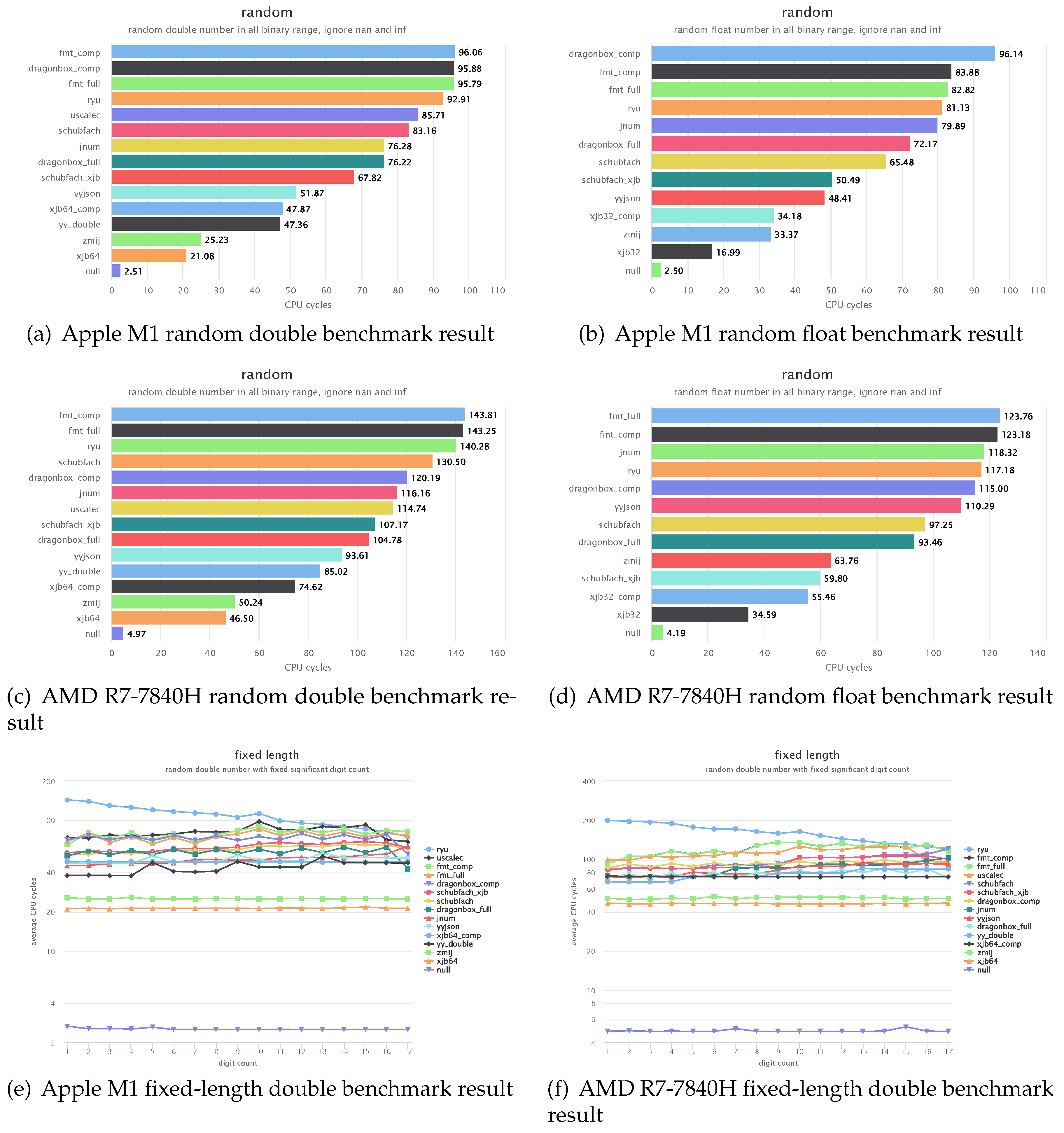
Table 2.
Valid ranges for significand c and exponent q
| Category | Float (binary32) | Double (binary64) |
|---|---|---|
| Subnormal | , | , |
| Normal | ||
| Irregular | , | , |
Table 3.
Example of floating-point number printing result.
| float number | fixed-point | scientific |
|---|---|---|
| 2.34 | “2.34” | “2.34e+00" |
| 12 | “12.0" | “1.2e+01" |
| 120 | “120.0" | “1.2e+02" |
| 0.012 | “0.012" | “1.2e-02" |
Table 4.
SIMD implementations of and
| SIMD implementation | Description |
|---|---|
| NEON [19] | Original author: Dougall Johnson. Runs on ARM processors with NEON instruction set. |
| SSE2 [20] | Based on scalar version; requires only SSE2 instruction set. |
| SSE4.1 | Nearly identical to SSE2 implementation; requires SSE4.1 instruction set. |
| AVX512 [21] | Original author: Daniel Lemire. Requires AVX512IFMA and AVX512VBMI instruction sets. |
Table 5.
Printing formats for different ranges.
| Type | Fixed-point | Scientific |
|---|---|---|
| float | other ranges | |
| double | other ranges |
Table 7.
Float/double to decimal benchmark results on AMD R7-7840H and ubuntu 26.04. The unit is nanosecond(ns).
Table 7.
Float/double to decimal benchmark results on AMD R7-7840H and ubuntu 26.04. The unit is nanosecond(ns).
| algorithm | float | double | |
|---|---|---|---|
| icpx 2025.0.4 | icpx 2025.0.4 | ||
| Schubfach | 12.2 | 11.51 | |
| Schubfach_xjb | 4.44 | 6.33 | |
| Ryu | 14.02 | 13.08 | |
| Dragonbox | 10.19 | 10.05 | |
| yy_json | 4.67 | 5.72 | |
| yy_double | - | 5.24 | |
| teju_jagua | 14.99 | 14.37 | |
| zmij | 4.76 | 4.78 | |
| uscalec | - | 11.27 | |
| xjb | 2.24 | 3.76 | |
Table 8.
Float/double to decimal benchmark results on Apple M1 and MacOS 26.4. The unit is nanosecond(ns).
Table 8.
Float/double to decimal benchmark results on Apple M1 and MacOS 26.4. The unit is nanosecond(ns).
| algorithm | float | double | |
|---|---|---|---|
| apple clang 21.0.0 | apple clang 21.0.0 | ||
| Schubfach | 11.64 | 13.12 | |
| Schubfach_xjb | 5.16 | 6.58 | |
| Ryu | 15.75 | 14.16 | |
| Dragonbox | 11.78 | 12.03 | |
| yy_json | 3.97 | 4.46 | |
| yy_double | - | 4.08 | |
| teju_jagua | 20.25 | 18.66 | |
| zmij | 4.11 | 3.83 | |
| uscalec | - | 15.26 | |
| xjb | 2.15 | 2.58 | |
Disclaimer/Publisher’s Note: The statements, opinions and data contained in all publications are solely those of the individual author(s) and contributor(s) and not of MDPI and/or the editor(s). MDPI and/or the editor(s) disclaim responsibility for any injury to people or property resulting from any ideas, methods, instructions or products referred to in the content. |
© 2026 by the authors. Licensee MDPI, Basel, Switzerland. This article is an open access article distributed under the terms and conditions of the Creative Commons Attribution (CC BY) license (http://creativecommons.org/licenses/by/4.0/).
Copyright: This open access article is published under a Creative Commons CC BY 4.0 license, which permit the free download, distribution, and reuse, provided that the author and preprint are cited in any reuse.


