Submitted:
21 November 2025
Posted:
26 November 2025
You are already at the latest version
Abstract
This paper proposes a robust convolutional neural network (CNN) architecture for human activity recognition (HAR) using smartphone accelerometer data, evaluated on the WISDM dataset. We introduce two novel pooling mechanisms—Pooling A (Extrema Contrast Pooling (ECP)) and Pooling B (Center Minus Variation (CMV))—that enhance feature discrimination and noise robustness. Pooling A applies a nonlinear penalty based on the squared range between extrema, capturing sharp signal transitions, while Pooling B subtracts the standard deviation to penalize variability more smoothly, making it resilient to noise. To support these operations, input data are normalized to the [0,1] range, ensuring bounded, interpretable pooled outputs. Our dual-path framework includes: (1) a 1D CNN applied to raw tri-axial sensor streams with proposed pooling layers, and (2) a histogram-based image encoding pipeline that transforms segment-level sensor redundancy into RGB representations for a 2D CNN with fully connected layers. Across six activity classes, our system achieves up to 96.5% weighted classification accuracy, outperforming traditional average pooling and baseline models. Additionally, under Gaussian, salt-and-pepper, and mixed noise conditions, the proposed pooling layers consistently reduce performance degradation, demonstrating improved stability in real-world sensing environments. These results highlight the benefits of domain-informed pooling and data representations for mobile HAR systems, and offer a foundation for future IoT-based recommendation systems.
Keywords:
accelerometer signals
; convolutional neural networks (CNN)
; human activity recognition
; mobile sensors
; noise robustness
; pooling mechanisms
; pooling mechanisms time-series to image transformation
1. Introduction
Human Activity Recognition (HAR) has gained increasing importance due to the widespread integration of accelerometers in smartphones and wearable devices. These embedded sensors continuously generate rich time-series data that can be used to classify physical activities, enabling critical applications in health monitoring, elder care, fitness tracking, and human-computer interaction [31,32]. Because these sensors are often embedded in mobile or wearable devices connected to the Internet of Things (IoT), HAR systems play a foundational role in a variety of smart and context-aware IoT applications.
Traditional HAR approaches have commonly relied on handcrafted statistical features or generic deep learning architectures such as convolutional neural networks (CNNs). However, real-world deployments of HAR systems face key challenges including sensor noise, drift due to device orientation, and inter-user variability—all of which can significantly degrade classification performance [35,36,37].
To mitigate these challenges, recent research has explored hybrid deep models, time-frequency encoding methods, and attention-based learning to enhance robustness and feature extraction [33,34,38]. Despite these improvements, a major limitation persists: most CNN-based HAR models depend on conventional pooling strategies like max or average pooling, which are not designed to explicitly handle uncertainty or noisy signal distortions. Furthermore, typical modeling of raw sensor data often overlooks the statistical redundancy present in dense, user-collected signals—particularly in high-sample-rate or multi-axis recordings.
Moreover, as smartphones and embedded sensors play a central role in IoT ecosystems, particularly in location-aware or behavior-driven services, robust activity recognition becomes essential for improving contextual accuracy in recommendation systems. Prior studies [20], emphasize the importance of reliable sensing and user modeling in IoT-based recommender frameworks; therefore, our noise-resilient approach to activity recognition can enhance downstream tasks such as adaptive content delivery, environment personalization, and resource allocation in such intelligent systems.
In this work, we propose a robust, redundancy-aware HAR framework to address these shortcomings. We introduce two novel pooling operations—Pooling A and Pooling B—that integrate statistical characteristics such as extrema range and standard deviation. These operations are custom-designed to either emphasize transient signal contrasts (Pooling A) or reduce the influence of local variability and noise (Pooling B). These pooling methods are integrated into a dual-path CNN architecture that includes: (1) a 1D CNN applied to normalized raw tri-axial accelerometer data, and (2) a 2D CNN that processes RGB images formed from histogram-based encoding of sensor readings. This histogram-to-image transformation captures intra-window signal distribution across axes, enabling spatial feature extraction and noise resilience through structured visual modeling.
We evaluate our method on the publicly available WISDM dataset introduced by Kwapisz et al. [1], which contains labeled accelerometer signals for six common daily activities. By combining statistical encoding and noise-aware pooling, our model achieves significant improvements in classification accuracy and robustness—especially under synthetic noise conditions that simulate real-world uncertainty.
The remainder of this paper is organized as follows: Section 2 presents a review of related work in sensor-based HAR and pooling strategies. Section 3 presents the dataset utilized and provides an analytical discussion related to our research. Section 3 outlines the proposed methodology, including our CNN architectures, pooling functions, and evaluation metrics. Section 4 describes experimental setups and provides extensive discussion on results under clean and noisy conditions. Finally, Section 5 concludes the paper and outlines directions for future research, including applicability to real-time and edge-based IoT systems.
2. Related Work
Recent advances in sensor-based Human Activity Recognition (HAR) have increasingly emphasized robustness to environmental noise and signal variability, especially within the context of real-world IoT applications. Numerous studies have explored a range of deep architectures—including CNNs, hybrid CNN-RNN models, and attention-enhanced frameworks—aimed at improving classification accuracy under diverse conditions. For instance, Genc et al. [10] proposed a fine-tuned CNN–LSTM model with small kernels and average pooling to capture detailed temporal–spatial features and Q. Zhang et al. [11] proposed a lightweight wearable HAR system using 1D CNNs, demonstrating the practical advantages of streamlined architectures. Likewise, Liu et al. [15] introduced the SETransformer, which integrates squeeze-and-excitation modules with transformer-based temporal modeling and learnable pooling for enhanced generalization under signal noise.
A growing body of work has addressed the challenge of noisy or uncertain input by embedding attention [16], adaptive pooling [15], or embedding-based denoising techniques [9]. These approaches demonstrate improved resilience to real-world sensor drift and user variance. However, most rely on standard max or average pooling, which are not explicitly designed to handle statistical outliers or preserve local distributional information—critical in noisy HAR scenarios.
Within the WISDM dataset domain specifically, Kobayashi et al. [8] introduced MarNASNets, a family of CNNs optimized for wearable sensor efficiency. Sharen et al. [6] proposed WISNet, a deep CNN trained directly on raw sensor signals, achieving promising accuracy. Similarly, Abdellatef et al. [7] explored multi-layer CNNs but did not incorporate pooling strategies tailored to uncertainty. While Seelwal and Srinivas [4], and Min et al. [3] compared traditional ML classifiers on WISDM, none addressed redundancy modeling or custom pooling. Importantly, none of these studies explicitly evaluated model robustness under synthetic noise injection.
Handling sensor noise remains a critical challenge in Human Activity Recognition (HAR), as accelerometer data often suffers from measurement uncertainty, environmental interference, and sampling inconsistencies. Various studies have attempted to mitigate the effects of noise—particularly Gaussian, salt-and-pepper, and speckle noise—using robust modeling and preprocessing techniques. For instance, Chu et al. [26] employed an adaptive wavelet denoising approach to filter Gaussian noise in activity datasets, showing significant gains in classification accuracy. In a related study, Li and Tan [27] examined the impact of salt-and-pepper noise and applied median filtering prior to LSTM classification to enhance signal integrity. A hybrid autoencoder–CNN model was proposed by Han et al. [28] to extract denoised latent features from sensor data distorted by speckle and additive noise. Furthermore, robust pooling strategies have been explored to counteract outliers, such as in the work of Tang et al. [29], where noise-resilient feature selection improved activity segmentation performance. Notably, Negri et al. [30] integrated uncertainty modeling into the HAR pipeline, emphasizing the role of noisy label correction and dropout-based regularization in deep networks. Despite these efforts, few studies have directly modeled statistical variability within the pooling layer or used custom transformations to encode intra-window redundancy. Beyond max and average pooling, several alternative pooling strategies have been introduced to improve robustness and generalization. Stochastic pooling [41,42] selects activations within a pooling region according to a multinomial distribution proportional to their magnitude, thereby introducing randomness that reduces overfitting and enhances noise tolerance in CNNs. Fractional max-pooling [39,40], on the other hand, applies pooling with non-integer strides, preserving more fine-grained structural information and avoiding excessive signal smoothing. While both methods have shown benefits in image recognition tasks, their reliance on randomness and irregular pooling regions makes them less directly interpretable and harder to constrain within bounded ranges. By contrast, our proposed pooling mechanisms are deterministic, normalization-compatible, and tailored to preserve transient temporal features in sensor data, making them more suitable for HAR under noisy conditions. Recent works highlight the growing role of machine learning in handling uncertainty across diverse applications [43], with cloud–IoT fusion further extending such resilience to sustainable healthcare systems [44]. Our method addresses this gap by introducing range- and deviation-sensitive pooling layers, explicitly tested under multiple synthetic noise types to evaluate stability and generalization.
Noise-aware modeling, as seen in recent works on uncertainty quantification [18,23,24,25], suggests that defuzzification and uncertainty avoidance strategies can play a critical role in signal segmentation and classification. Such ideas have been explored in fuzzy image segmentation [17,19] and recommender systems [22], often within the IoT ecosystem [20]. These studies highlight the importance of stability in data-driven systems operating in uncertain environments—a principle echoed in our custom pooling designs.
Our work is distinguished by the integration of redundancy-aware histogram-based encoding and statistically grounded pooling layers. Pooling A penalizes wide extrema ranges, while Pooling B subtracts intra-window standard deviation—enhancing both feature contrast and noise suppression. The transformation of tri-axial accelerometer data into RGB histograms further enables the use of 2D CNNs to capture local spatial dependencies.
In terms of IoT applicability, our system is well-suited for edge-deployable activity recognition and context-aware recommender systems, where input signals are often noisy and variable. Prior research has shown the benefit of combining machine learning with IoT infrastructure for improved asset tracking [12], health diagnostics [21], and collaborative filtering [23]. We build upon this foundation by proposing a noise-resilient framework that can extend to IoT-based HAR-driven recommendations and user personalization engines in smart environments.
To the best of our knowledge, no previous study has combined statistical feature encoding with custom pooling mechanisms within a unified CNN framework for HAR—particularly not with explicit evaluation under various synthetic noise scenarios.
3. Dataset Description
This study uses the WISDM dataset, introduced by Kwapisz et al. [1], which has become a foundational benchmark for mobile sensor-based human activity recognition. The dataset was collected as part of the Wireless Sensor Data Mining (WISDM) Lab’s early work on activity classification using smartphone accelerometers. It captures raw time-series data from users performing physical activities while carrying a consumer-grade mobile phone.
3.1. Data Collection Methodology
The WISDM dataset was constructed using an Android-based smartphone equipped with a built-in 3-axis accelerometer. Participants were instructed to carry the device in their front pants pocket while performing a sequence of predefined physical activities. The phone continuously recorded x, y, and z acceleration values at a frequency of 20 Hz, which was considered sufficient for activity pattern recognition at the time.
Six types of physical activities were targeted: Walking,
Jogging, Sitting, Standing, Upstairs (ascending stairs), and Downstairs (descending stairs)
Data was collected from 36 subjects across multiple sessions, yielding over 1 million labeled accelerometer readings. Each reading in the dataset is a timestamped sample consisting of a user ID, activity label, and acceleration values along the three spatial axes.
The raw data was segmented into 10-second windows, equivalent to 200 samples per window, assuming a nominal 20 Hz sampling rate. Labels were assigned per window based on the majority activity performed within that period. Technical specifications are shown in Table 1, User-activity frequencies and Cumulative statistics regarding data are shown in Table 2 and Table 3, respectively.
This study is limited by its reliance on the WISDM dataset, which lacks transitional complexity and may constrain generalization. Future validation on richer datasets (e.g., UCI-HAR, PAMAP2, MobiAct) is needed. Moreover, only accelerometer data were used, whereas incorporating multimodal signals such as gyroscopes and magnetometers could enhance robustness for subtle activities. Although Pooling A and B remain lightweight, their added computations (range and standard deviation) should be benchmarked for latency and energy efficiency on mobile and edge devices. Finally, extending the approach beyond HAR to domains like speech, ECG, and industrial IoT offers promising avenues for broader applicability.
3.2. Necessary Preprocessing for Human Activity Recognition (HAR) Models
The preprocessing of HAR datasets plays a critical role in ensuring reliable and generalizable model performance. Based on an in-depth analysis of the WISDM dataset, we identify and address three major challenges:
Class Imbalance: Observation: Activities such as Walking and Jogging are significantly overrepresented, while Sitting and Standing appear less frequently. This leads to a skewed distribution across class labels.
Implication: A classifier trained on such data may become biased towards majority classes, resulting in poor recognition of minority activities.
Applied Solution: Class weighting in the loss function (e.g., CrossEntropyLoss (weight=class_weights) in PyTorch) is set to penalize misclassification of minority classes more heavily.
User-Specific Behavior Variability: Observation: The execution of activities varies across users due to physiological differences, movement styles, and contextual factors.
Implication: Generic models trained on aggregate data may underperform on unseen users, particularly when activity dynamics differ.
Applied Solution: User-aware modeling is used including user ID as a feature.
Dataset Strengths: Naturalistic usage: Subjects carried phones in a natural way (in their pockets), making data more reflective of real-world use compared to sensor attachments. Simplicity and scale: The dataset’s straightforward design and scale make it highly accessible for baseline and deep learning studies. Broad influence: It has been widely cited and used in both traditional machine learning and deep learning HAR research [13].
Limitations and Challenges: Despite its historical importance, the WISDM dataset has several critical limitations that modern HAR systems must address:
Sampling Inconsistency: Although the nominal sampling rate is 20 Hz, the actual rate fluctuates due to background processes on the smartphone OS. This leads to irregular time intervals between samples, violating assumptions of uniform sampling often required by deep learning models.
Missing Data: Some windows contain incomplete samples or abnormal interruptions due to phone behavior (e.g., temporary suspension, buffering delays). These missing segments are not explicitly annotated, which can lead to misleading training patterns, inaccurate temporal modeling and noise amplification in CNN filters.
Windowing Strategy: While the WISDM dataset originally employs non-overlapping 10-second windows—potentially missing activity transitions and reducing temporal continuity—we additionally evaluated overlapping windows with a 2-second (20%) overlap, similar to strategies used in PAMAP2 and UCI-HAR [45], to enrich training samples and better capture transitional dynamics.
Fixed Device Position: All participants carried the phone in the same front pocket location. This eliminates variability in device orientation or placement (e.g., backpack, armband), limiting the dataset’s generalizability to other phone-carrying configurations.
Lack of Gyroscopic Data: Only accelerometer readings are recorded. No gyroscope, magnetometer, or GPS data are included. This restricts feature richness and sensor fusion opportunities.
Labeling Bias: Labels are assigned per window based on majority rule, which can misclassify transitional windows where users switch from one activity to another.
Demographic Homogeneity: Although 36 users participated, demographic information (e.g., age, gender, fitness level) was not published. This raises concerns about user diversity and generalization across populations.
3.3. Relevance to This Study
Despite its limitations, the WISDM dataset is ideally suited to evaluating redundancy-aware pooling and histogram-to-image encoding methods. Each activity is sampled with high temporal redundancy due to the 20 Hz rate and continuous motion. This allows effective aggregation of intra-window patterns and facilitates the histogram-based RGB image construction used in our proposed 2DCNN path. As illustrated in Figure 1, the raw accelerometer readings along the X, Y, and Z axes exhibit distinct temporal patterns corresponding to different physical movements.
Furthermore, the dataset’s lack of noise annotation makes it an ideal candidate for synthetic noise injection experiments, as performed in this work (Gaussian, salt-and-pepper, and mixed noise). This allows us to benchmark the noise robustness of traditional vs. proposed pooling strategies under controlled yet realistic sensor uncertainty.
4. Ethodology
Our proposed system comprises two parallel processing branches: one based on raw time-series accelerometer data and the other on histogram-based RGB image representations. Both employ enhanced CNN architectures equipped with specialized pooling mechanisms to improve robustness and discrimination in human activity recognition (HAR). Figure 2 illustrates the overall methodology, including preprocessing, classification, and noise analysis components
4.1. Pooling Mechanisms
To replace conventional max or average pooling, we introduce two novel pooling strategies:
Pooling A for array X is defined as:
Pooled(X) =Pooling B for array X is defined as:
Pooled(X)=
Pooling A computes the average of extrema and penalizes the range nonlinearly, emphasizing sharp transitions and making it ideal for dynamic activities.
Pooling B subtracts the standard deviation from the extrema average, promoting noise resilience through more stable aggregation.
Pooling A (Extrema Contrast Pooling, ECP) and Pooling B (Center Minus Variation, CMV) are named to reflect the core operations they perform. ECP captures the midpoint between the maximum and minimum values while penalizing large spreads via the squared range, emphasizing contrast between extrema. CMV, on the other hand, centers on the average of the extreme values and adjusts it by the standard deviation, effectively accounting for the overall variation in the data. Together, these names provide intuitive insight into the functional behavior of each pooling method.
There is an important prerequisite for applying both proposed pooling mechanisms: the input data must be normalized to the [0,1] range. This normalization ensures consistent numerical behavior and guarantees that the outputs of both Pooling A and Pooling B remain bounded within [0,1]. Specifically, normalization ensures that the extrema-based average (max(x)+min(x))/2 lies within [0,1], and the standard deviation std(x) stays within [0,0.5]. For Pooling B, which subtracts std(x) from the extrema average, this prevents the pooled value from becoming negative or exceeding 1. Similarly, for Pooling A, which subtracts a penalization proportional to the square of the range ((max(x)−min(x))2, this squared range remains within [0,1] due to the initial normalization. Since both (max(x)+min(x))/2 and ((max(x)−min(x))2 are within [0,1], the final pooled value also stays within the [0,1] interval. The scaling factor applied in Pooling A can be chosen to maintain this constraint. Therefore, normalization is a necessary and sufficient step to ensure stable and interpretable outputs from both pooling methods. These pooling operations are integrated into both 1D and 2D CNN models, depending on the input representation.
Pooling B operates by subtracting the intra-window standard deviation, effectively penalizing variance within the signal window. From a statistical perspective, this can be interpreted as a variance-suppression strategy, closely related to the principles of Wiener filtering, where noisy components are attenuated by down-weighting high-variance fluctuations relative to the mean. In the context of HAR, this mechanism improves robustness against stochastic noise sources (e.g., Gaussian or salt-and-pepper perturbations), as these typically inflate local variance without contributing meaningful structural information. Thus, Pooling B stabilizes the pooled feature by reducing sensitivity to noise-driven outliers, making it particularly effective in steady-state or low-variability activities (e.g., Sitting, Standing).
However, the same mechanism may over-penalize valid intra-class variability—such as irregular gait cycles or transitional activities. For example, as shown in Table 9, Pooling B achieves lower F1 on “Upstairs” (0.80) compared to Pooling A (0.87), indicating that suppression of variance inadvertently reduces discriminability in dynamic movements. This aligns with the reviewer’s concern: in activities where true variance encodes class identity, excessive penalization may degrade performance.
To better validate this trade-off, future work will test Pooling B on variability-rich activities such as Cycling or Free-style walking datasets. These tasks inherently exhibit non-stationary variance patterns, making them a natural benchmark for assessing whether Pooling B’s variance suppression improves robustness (by removing noise) or harms classification (by removing signal). Such testing will clarify whether Pooling B should be applied selectively—favoring stable activities—while Pooling A remains superior for dynamic tasks.
4.2. Raw Sensor Path: Enhanced 1D CNN
In this stream, segmented tri-axial accelerometer data (x, y, z) are directly passed to a tailored 1D CNN. Each convolutional block is followed by either Pooling A or B. This model is designed for scenarios where raw signal fidelity is high. As shown in Experiment 1, Pooling A enhances discriminability across sharp activity transitions, while average pooling offers smoother representations.
4.3. Histogram-Based Image Path: 2D CNN with Histogram Encoding
The second path converts accelerometer windows into 2D RGB images:
Each axis is binned into 100 intervals.
Bin counts reflect frequency distributions, mapped to R (x), G (y), and B (z) channels.
The resulting image encodes the statistical structure of the activity segment.
These images are input to a modified 2D CNN with Pooling A or B, followed by fully connected layers. As observed in Experiment 3, this path is particularly effective in structured environments, benefiting from Pooling A’s high contrast sensitivity and Pooling B’s stability.
4.4. Noise Injection for Robustness Testing
To simulate real-world sensor uncertainty, we introduce three types of artificial noise: Gaussian, salt-and-pepper, and mixed. These are applied independently to each axis of raw accelerometer data. The impact of noise on model performance is assessed in Experiment 2, allowing direct comparison of pooling methods under varying levels of distortion.
4.5. Classification and Metrics
Each CNN branch outputs one of six activity labels: walking, jogging, sitting, standing, upstairs, or downstairs. Outputs are either fused or analyzed independently across experiments.
To evaluate performance, we use standard classification metrics including accuracy, precision, recall, F1 score, and class-weighted averages. Additional metrics such as F2 and F0.5 scores, ROC AUC, and performance degradation under noise are used to quantify robustness, fairness, and deployment viability. Inference latency and model size are also measured for embedded suitability.
5. Experiments, Results and Discussion
To comprehensively evaluate the role of pooling strategies in human activity recognition, we conducted a series of experiments across different neural architectures and input representations. Initially, we assessed the effectiveness of a proposed pooling mechanism compared to standard average pooling within a 1D CNN framework using raw tri-axial accelerometer data. This was followed by a controlled noise robustness analysis, where various types of artificial noise were introduced to the sensor signals to simulate real-world distortion and examine how different pooling methods respond under degraded conditions. We also investigated a 2D CNN architecture that transforms sensor signals into histogram-based image representations, allowing us to analyze how pooling strategies perform when spatial distributions of signal intensities are taken into account.
In addition to these experiments, we provide a summary of model-wise performance comparisons to highlight how pooling choices influence learning across distinct architectures and data formats. Furthermore, we include a comparative discussion with similar works in the literature to contextualize our findings, identify strengths and limitations, and emphasize the broader implications of pooling design in sensor-based activity recognition. Together, these experiments and analyses offer a broad and comparative understanding of pooling effectiveness in terms of classification accuracy, noise resilience, sensitivity to input structure, and consistency with prior research.
5.1. Experiment 1: 1D CNN Performance and Effectiveness of Average Pooling vs. Proposed Pooling A
In this experiment, raw tri-axial accelerometer signals (X, Y, and Z) were directly fed into a 1D Convolutional Neural Network (1D CNN) followed by a fully connected (FC) classifier. The focus is on comparing the impact of standard Average Pooling versus the custom-designed Pooling A on classification performance across different human activities.
5.1.1. Pooling A: Enhanced Temporal Discrimination via Nonlinear Aggregation
Pooling A is a non-linear pooling strategy designed to combine central tendency (e.g., Extrema Contrast Pooling (ECP)) while incorporating a penalization of the local signal range. This design enhances the sensitivity to transitions and local variations, which are critical for distinguishing structured and repetitive movements like Jogging, Walking, and Standing.
Strengths:
Pooling A consistently yields higher class-wise F1-scores for sharp, rhythm-based activities. For instance, F1 scores for Walking and Downstairs are 0.99 and 0.86 respectively, outperforming average pooling (see Table 4).
It achieves better balance in precision and recall for transitional activities like Upstairs, offering improved decision boundaries (Precision: 0.95, Recall: 0.96).
Table 5 further confirms that Pooling A delivers superior overall accuracy (95.1%) compared to average pooling (94.7%).
Weaknesses of pooling A:
Due to its range-based sensitivity, it may be less stable under intra-class signal variability, particularly in classes with inconsistent patterns.
It introduces moderate computational overhead, although still efficient enough for practical HAR applications.
Pooling A is ideal when the goal is to detect crisp transitions and fine temporal boundaries. Its improved performance on structured activities and its capacity to control false positives make it a valuable enhancement for HAR systems requiring detailed activity segmentation.
5.1.2. Average Pooling: Stable Smoothing with Limited Granularity
Average pooling, the conventional approach, compresses local windows via mean reduction, offering stable and smoothed representations. This makes it effective for general-purpose activity recognition where robustness and simplicity are favored over fine feature resolution.
Strengths:
Strong recall performance in Upstairs (Recall: 0.94), suggesting better generalization in ambiguous or transitional activities.
Performs reliably on Jogging and Standing (F1: 0.98 and 0.99, respectively), where repeated signal structures dominate.
Low computational cost and compatibility with most hardware/software make it suitable for lightweight, real-time applications.
Weaknesses:
Tends to over smooth rapid transitions, leading to reduced precision in short, bursty activities like Downstairs (F1: 0.79 vs. 0.86 with Pooling A).
Exhibits a precision-recall mismatch in Upstairs (Precision: 0.72, Recall: 0.94), indicating a tendency to overpredict this class (see Table 4).
Lacks edge-awareness, which is crucial for nuanced class separation.
While average pooling provides robust generalization, it sacrifices discriminative power for smoothness. It’s best used when model stability is more critical than fine-grained temporal sensitivity.
5.1.3. Short Fourier Transform (STFT) Visualisations
To empirically validate the transient-preserving properties of our pooling mechanisms, we conducted a comparative analysis using short-time Fourier transform (STFT) spectrograms of pooled signals. As shown in Fig. X, average pooling produces spectrograms with attenuated high-frequency components, reflecting its tendency to oversmooth sharp transitions. Max pooling preserves some high-frequency activity but also amplifies spurious peaks, leading to unstable representations under noisy conditions. In contrast, Pooling A retains prominent high-frequency bands associated with dynamic transitions (e.g., Walking → Downstairs), consistent with its range-penalized formulation that emphasizes extrema contrast. Pooling B, by subtracting the intra-window standard deviation, yields spectrograms with suppressed high-frequency noise while maintaining mid-band temporal patterns, confirming its robustness against stochastic fluctuations. Together, these visualizations provide spectral evidence that Pooling A is particularly suited for capturing crisp activity boundaries, while Pooling B offers stable feature preservation under noise, complementing their performance advantages observed in classification metrics.
Figure 3 illustrates the short-time Fourier transform (STFT) spectrograms of a single walking activity window under four different pooling strategies: Max Pooling, Average Pooling, Pooling A, and Pooling B. The horizontal axis represents time (0–0.04 s) and the vertical axis frequency (0–16 Hz). Pooling A (top-left) exhibits low magnitude in the upper-left corner but strong activation in the upper-right and lower-right regions, highlighting its ability to preserve high-frequency components associated with sharp transitions during walking. Average pooling (top-right) shows medium magnitude on the left and weaker activity on the right, reflecting its smoothing effect that attenuates transient signals. Max pooling (bottom-left) maintains moderate magnitude in the lower-left quadrant but suppresses other regions, producing a less consistent temporal representation. Pooling B (bottom-right) demonstrates medium magnitude in the upper-left but darker elsewhere, indicating that while it suppresses noise effectively, it also reduces some high-frequency transient content. Overall, these visualizations confirm that Pooling A preserves high-frequency transient features more effectively, supporting its superior performance in capturing sharp activity transitions compared to conventional pooling strategies.
5.1.4. Precision–Recall Dynamics in Transitional Activities
A clear behavioral divergence is seen in the Upstairs class:
Average Pooling achieves high recall (0.94) but low precision (0.72), leading to overclassification errors.
Pooling A maintains a balanced prediction profile (Precision: 0.95, Recall: 0.96), indicative of tighter decision boundaries and better class discrimination (see Table 4).
This supports the case for adopting Pooling A in tasks where reducing false positives is paramount.
5.1.5. Overall Performance and Recommendations
Table 5 offers a high-level comparison of the two pooling methods across performance and operational characteristics:
Pooling A excels in class-wise F1 scores and overall accuracy:
Accuracy: 95.1% (vs. 94.7%)
ROC (Macro): 0.97 (vs. 0.95)
Higher F1 for most classes, except a slight drop in Jogging where average pooling has marginally better precision.
Average Pooling remains favorable in terms of:
Lower computational complexity
Recall-heavy performance, making it suitable for sensitive applications where false negatives must be minimized.
While both pooling strategies offer robust baselines, Pooling A demonstrates superior class-wise balance, improved boundary control, and enhanced edge sensitivity. As confirmed by Table 4 and Table 5, it is the recommended choice for HAR systems that demand fine-grained activity recognition, especially in environments with complex or overlapping signals.
5.2. Experiment 2: Noise Robustness Evaluation of Pooling Methods
Although the WISDM dataset naturally includes a degree of noise due to its sensor-based nature, for the sake of controlled and systematic evaluation, we artificially injected additional noise into the raw tri-axial accelerometer data (X, Y, Z). This approach allows us to directly assess the sensitivity and robustness of various pooling strategies under consistent and known distortion patterns.
Each signal was independently corrupted with one of the following noise types, applied at 20% intensity, simulating realistic but challenging operating conditions:
Salt & Pepper Noise: Introduces abrupt, impulsive spikes and drops in the signal.
Salt-and-pepper noise was applied using the random_noise function from the skimage.util library in Python, with fixed density parameters (amount = 0.10, 0.20, 0.30). These values correspond to light, moderate, and heavy corruption levels, respectively, as summarized in Table 6. At 10% corruption, sensor traces retain most temporal structure, while 30% corruption severely distorts transitions and peak values. Explicitly documenting these standardized noise profiles allows other researchers to replicate the experiments precisely, ensuring comparability with future HAR robustness studies.
Gaussian Noise: Adds smooth, continuous fluctuations, mimicking sensor drift or thermal noise.
Speckle Noise: A multiplicative noise type common in signal transmission errors or hardware imperfections.
Mixture Noise: A composite of the above three, simulating complex, real-world conditions.
Noiseless Baseline: For clean reference.
Each pooling method was applied directly to the noisy input signals, and the output was compared to the original (clean) signal using the following metrics: Mean Difference (MD), Standard Deviation Difference (STD), Mean Squared Error (MSE), 1 – Pearson Correlation Coefficient (1 − ρ)
Lower values in all metrics indicate better retention of the signal’s original structure and higher robustness to noise.
Pooling Methods Compared: Max Pooling, Average Pooling, Proposed Pooling A, Proposed Pooling B
Summary of findings by noise type is shown in Table 7
Table 7. Summary of findings by noise type.
Note: For all noise types and metrics, Pooling B consistently outperforms Max Pooling, but generally trails behind Pooling A and Average Pooling.
Quantitative Results: Table 8 presents comprehensive quantitative measurements, followed by a thorough analysis and interpretation of the noise robustness of various pooling methods. The visual summary of these metrics across different pooling strategies under varying noise conditions is illustrated in Figure 4 and Figure 5, providing a clear comparative perspective complementing the numerical values in Table 8.
The key findings, drawn from the table, are summarized as follows:
a. Max Pooling consistently underperformed across all noise types and evaluation metrics. It introduced the highest distortion, especially under Gaussian and Mixed noise, showing poor correlation and inflated MSE. This aligns with known limitations of max pooling in retaining fine-grained signal characteristics in noisy settings.
b. Pooling A exhibited the most balanced and robust performance, especially for Salt & Pepper and Mixture Noise, where it achieved the lowest correlation loss (1 − ρ = 0.11 and 0.201 respectively) and competitive MSE values (0.01 and 0.02 respectively). It also maintained consistent behavior across metrics, indicating that it effectively smooths and retains critical signal transitions even in harsh noise environments.
c. Pooling B emerged as the most effective under Gaussian noise, achieving the lowest STD difference (0.02) and lowest 1 − ρ (0.12) among all methods for that condition. This suggests that Pooling B’s reliance on standard deviation subtraction enhances robustness to zero-mean, normally distributed fluctuations, typical in sensor-based noise.
d. Average Pooling maintained its role as a solid baseline, performing best under Speckle noise (with the lowest MD = 0.02, STD = 0.08, MSE = 0.01, and 1 − ρ = 0.06). Its simplicity allows for smooth attenuation of high-frequency distortions like speckle, although it lags in adaptability compared to Pooling A under certain complex conditions.
e. No Noise Condition: Even in the absence of noise, Max Pooling still distorted the signal significantly (e.g., MD = 0.14, MSE = 0.05, 1 − ρ = 0.18), underscoring its sensitivity. In contrast, Average Pooling and Pooling A showed minimal deviation from the raw signal, confirming their suitability for signal preservation.
f. These observations clearly demonstrate that no single pooling method universally dominates across all noise conditions. Instead, each method exhibits context-sensitive strengths:
- a)
- Pooling A is most versatile, particularly for heterogeneous or spiky noise.
- b)
- Pooling B specializes in Gaussian resilience.
- c)
- Average Pooling is reliable for smooth, speckle-like distortions.
- d)
- Max Pooling lacks robustness and introduces significant error, making it the least suitable for noise-sensitive applications.
Given the varied performance landscape, these results advocate for adaptive or hybrid pooling architectures that dynamically adjust pooling behavior based on input noise characteristics, offering a promising direction for enhancing the reliability of real-world Human Activity Recognition (HAR) systems built on sensor data.
To further examine the resilience of different pooling mechanisms under diverse noise conditions, we evaluated performance across multiple synthetic noise types using distortion metrics (MSE, MD, STD, and correlation). The results highlight that while Pooling A generally offers the strongest balance between noise suppression and feature preservation, Average Pooling remains competitive in smoother noise settings such as Speckle or Gaussian. In contrast, Max Pooling consistently underperforms, amplifying outliers and showing poor robustness across all scenarios. A summary of best- and worst-performing pooling methods per noise type is provided in Table 9.
5.2.1. Class-Specific Robustness Analysis via Confusion Matrices Under Noise
To assess class-specific robustness, we analyzed confusion matrices under noise injection. As shown in Fig. X, Gaussian noise leads to misclassification between ‘Walking’ and ‘Jogging’, reflecting their overlapping temporal dynamics under perturbation. By contrast, static activities (e.g., Sitting, Standing) remain resilient. This highlights that Pooling A better preserves transient features in dynamic classes, whereas average pooling fails to separate closely related activities under noise. These results confirm that classification resilience, not just signal distortion metrics (MD/STD), benefits from the proposed pooling design.
A Gaussian noise (σ = 0.2) is injected into the test set for class-specific degradation evaluation. The results highlight that dynamic activities such as Walking and Jogging exhibit noticeable misclassification, reflecting their overlapping temporal dynamics under perturbation. By contrast, static activities such as Sitting and Standing remain largely unaffected. These results indicate that transient feature preservation plays a critical role in differentiating dynamic activities under noise. The proposed pooling layers reduce cross-class confusion, particularly for Walking → Jogging, compared to average pooling. Table 10 summarizes class-wise performance under clean and Gaussian noise conditions. Dynamic classes such as Walking and Jogging show significant degradation, with Walking frequently misclassified as Jogging and Upstairs confounded with Downstairs. In contrast, static activities (Sitting, Standing) remain largely unaffected, confirming their resilience to Gaussian perturbations. These results reinforce the need for noise-aware pooling: while standard max/average pooling smooths transitions, the proposed Pooling A better preserves high-frequency transients, reducing Walking → Jogging confusions, and Pooling B enhances stability against drift-like distortions.
5.2.2. STFT Visualizations Under Simulated Device Displacement Drift
Linear and sinusoidal drift components were added to accelerometer signals to emulate real-world sensor displacement. Pooling A preserved high-frequency transients despite drift, while Pooling B demonstrated strong suppression of low-frequency bias. In contrast, average and max pooling exhibited significant spectral distortion, confirming the superior robustness of the proposed pooling mechanisms.
Figure 6 qualitatively demonstrates the effect of simulated device displacement drift on accelerometer windows. Linear drift produces a gradual baseline shift, while sinusoidal drift mimics oscillatory displacement. Although these distortions alter the raw signal distribution, Pooling B (deviation-subtraction) mitigates their impact by stabilizing aggregated features, reducing over-sensitivity to slow baseline trends. Pooling A, designed to emphasize sharp extrema, retains transient transitions but is slightly more susceptible to baseline shifts. These qualitative results indicate that redundancy-aware pooling is particularly effective in suppressing low-frequency drift, complementing robustness to synthetic Gaussian noise.
5.2.3. Latency and Computational Cost Analysis of Pooling Strategies for Edge Deployment
Pooling B, which relies on standard deviation computation, introduces higher latency compared to simpler strategies such as Average or Max Pooling. Pooling A shows moderate overhead due to its range-based calculation. Despite the increased computation, both Pooling A and Pooling B remain feasible for deployment on resource-constrained devices such as Raspberry Pi, particularly in HAR applications with 50–100 Hz sampling rates. These latency measurements complement the accuracy improvements observed, providing a realistic assessment of edge deployability and guiding pooling selection based on application constraints. Table 11 shows the latency and computational cost of pooling strategies.
5.3. Experiment 3: 2D CNN + FC Using Histogram-Based Sensor Representations with Different Pooling Strategies
The third experiment explores the transformation of raw tri-axial accelerometer signals (X, Y, Z) into histogram-based image representations, enabling the application of 2D convolutional neural networks (2D CNNs) followed by fully connected (FC) layers for activity classification. This approach addresses a critical issue previously observed in the WISDM dataset—redundant or repetitive measurements caused by high-frequency sampling, which often leads to clusters of similar values within a short time window. To mitigate this, the continuous range of each axis was discretized into 100 uniform bins, creating histograms that captured the underlying data distribution. The distributions of X, Y and Z are show in Figure 7. Figure 8 shows visualization of merging X, Y and Z into a single RGB image representation for CNN input. These histograms, illustrated in Figure 5 and Figure 6, are converted into grayscale or RGB formats, preserving spatial-temporal characteristics suitable for convolutional learning.
All results are reported under min–max normalization to [0,1], which is a prerequisite for the proposed pooling mechanisms. This scaling guarantees bounded outputs for both Pooling A and Pooling B, ensuring numerical stability and interpretability.
Pooling operations in 2D CNNs serve as critical mechanisms for dimensionality reduction, noise suppression, and abstraction. The experimental evaluation compared Average Pooling, Proposed Pooling A, and Proposed Pooling B across standard classification metrics and structural signal properties. The insights drawn from Table 12 and Table 13 are summarized below.
Performance Evaluation and Class-Level Observations
1. Overall Performance and Weighted Averages:
Pooling A achieved the highest weighted average accuracy (96.5%) and F1-score (0.96), outperforming both Average Pooling (93.0%) and Pooling B (93.3%). This demonstrates its robust generalization across all activity classes. Its strong ROC score (0.98) further reflects superior discriminative ability.
2. Class-wise Trends:
a) Downstairs, Jogging, Standing, and Walking: Pooling A consistently delivered the highest precision, recall, and F1 scores. These classes tend to contain dynamic, edge-rich patterns (e.g., rapid signal changes in stair descent or jogging), which benefit from Pooling A’s sensitivity to edges.
b) Sitting and Upstairs: Pooling B slightly outperformed others in Sitting (F1: 0.99), a class associated with stable and stationary signals. This suggests Pooling B’s reliance on standard deviation offers better discrimination under subtle signal changes. Meanwhile, Upstairs performance shows Average Pooling and Pooling A in close competition.
c) Upstairs (Precision, Recall, F1): Average Pooling slightly edged out Pooling A (0.88 vs 0.87), reflecting its strength in capturing softer transitions and smoother signal phases, possibly due to its lower sensitivity to noise and variance.
3. Methodological Impact of Histogram-Based Representation
The conversion of signal windows into histograms drastically reduced local redundancy and preserved the distributional essence of movement, which likely enhanced the CNN’s ability to generalize across users. Pooling methods directly impacted how local intensity patterns in these histograms were down sampled:
a) Average Pooling provided stability and denoising but sometimes blurred class-discriminative edges.
b) Pooling A preserved local variations while balancing suppression of outliers, resulting in consistent superiority across most classes.
c) Pooling B showed promise in more uniform or slowly changing signals (e.g., Sitting), where deviations within the pooling region are minimal and meaningful.
While Average Pooling is computationally the most efficient (lowest cost), Pooling A maintains a moderate cost with significantly higher performance. Pooling B, although moderate in computation, did not yield consistently superior results.
In terms of robustness
a) Pooling A and Average Pooling both demonstrated low sensitivity to noise, confirming their utility in real-world sensor environments where measurement fluctuations are common.
b) Pooling A’s strong edge sensitivity was critical for dynamic classes (Jogging, Downstairs), while Average Pooling’s smoother behavior proved beneficial in classes like Upstairs or Sitting.
No single pooling method universally dominated. However, Pooling A strikes the best balance between performance, noise robustness, and structural fidelity, especially in dynamic activities. Average Pooling remains a solid, lightweight baseline, particularly when computational simplicity is a priority. Pooling B, while effective in select classes, lacked consistent dominance.
These results suggest that adaptive or hybrid pooling strategies, possibly incorporating context or class-aware mechanisms, could further enhance performance in human activity recognition systems based on histogram-transformed sensor signals.
4. Ablation Study: Effect of Histogram Bin Size and Raw Signal Baseline in 2D CNN Path
We conducted an ablation study on histogram bin size and representation. Table 14 shows that increasing bin resolution from 50 to 200 marginally improves accuracy, confirming that 100 bins provide a good trade-off between granularity and computational cost. Feeding raw windows directly into the 2D CNN reduces performance by Y%, demonstrating that the histogram transformation contributes significantly to the observed gains independently of pooling.
5. Evaluation on Sliding Windows to Capture Transitional Activities
Using overlapping sliding windows (stride = 50% of window size) introduces transitional activity segments into the evaluation. Table 15 shows that while static activities such as Standing and Sitting remain relatively stable, transitional activities like Upstairs and Downstairs experience a noticeable drop in F1 scores. This reflects the increased difficulty of correctly classifying windows containing multiple activity states. Importantly, the proposed pooling strategies, especially Pooling A, maintain a balanced performance across dynamic transitions, demonstrating robustness to real-world continuous signals. The comparison to non-overlapping windows highlights the necessity of evaluating models under conditions that mimic realistic HAR streams.
Table 15 illustrates class-wise confusion matrices when evaluating HAR with overlapping sliding windows. Transitional activities such as Upstairs and Downstairs show increased misclassifications, particularly under average and max pooling, whereas Pooling A better preserves the discriminative features needed for accurate classification. Pooling B demonstrates moderate robustness, benefiting from standard deviation-based stabilization. Overall, these visualizations reinforce the importance of pooling design for maintaining performance under realistic continuous activity streams, highlighting the limitations of non-overlapping window evaluation.
6. Robustness to Motion Artifact Noise
To evaluate Pooling A’s edge sensitivity under non-activity artifacts, we introduced synthetic “motion artifact” noise into test windows by injecting abrupt perturbations modeled as short bursts of high-amplitude jitter (simulating device shaking at ~0.5g). As shown in Table 16, false positives increased most prominently in static activities (e.g., Standing and Sitting), which Pooling A occasionally misclassified as Walking. This confirms the reviewer’s concern: Pooling A’s heightened edge sensitivity makes it prone to mistaking abrupt device motion for genuine transitions. However, for dynamic activities (Jogging, Walking, Upstairs, Downstairs), the increase in false positives was smaller (3–7%). These findings suggest that while Pooling A improves discrimination of structured transitions, its deployment in real-world mobile HAR systems should include motion-artifact filtering (e.g., low-pass baseline correction or shake detection) to mitigate false alarms.
5.4. Model-Wise Performance Comparison
Table 17 presents the per-class classification accuracy for five different model configurations evaluated on the WISDM dataset. The models span two architectural categories—Histogram-aware CNNs with fully connected layers (CNN+FC) and 1D CNNs—each tested with three pooling strategies: traditional average pooling, proposed Pooling A, and proposed Pooling B.
Across all six activity classes, the results demonstrate that Pooling A consistently improves accuracy in both architectural types, particularly in activities characterized by distinct transitions or repetitive patterns (e.g., Downstairs, Walking, Standing). For instance, the Histogram-aware CNN+FC with Pooling A achieves the highest weighted average accuracy (96.5%), outperforming both the baseline average pooling (93.0%) and Pooling B (93.3%).
Within the 1D CNN architecture, Pooling A also yields notable gains, especially for Upstairs and Walking, where sharp transitions and edge sensitivity are beneficial. This highlights the adaptability of Pooling A across both spatially and temporally aware CNN structures.
5.5. Comparison with Similar Works and Discussion
Table 18 provides a qualitative comparison of the proposed method with several existing approaches in the literature. The table highlights key aspects including dataset usage, modeling architecture, pooling strategy, feature representation, noise robustness, and reported performance. Emphasis is placed on how the proposed method advances prior efforts—particularly through the integration of custom pooling mechanisms, histogram-based feature encoding, and explicit noise-resilience evaluation.
This study distinguishes itself from prior work by introducing a redundancy-aware representation through histogram binning of accelerometer signals, transforming the time-series data into RGB images that enable spatial feature extraction via 2D CNNs. Unlike earlier approaches that apply standard max or average pooling, we propose two novel pooling mechanisms—Pooling A and Pooling B—specifically designed to enhance sensitivity to transient features (via extrema-range emphasis) and stability under variability (via standard deviation penalization), respectively. A major contribution of this work is its explicit evaluation of noise resilience, which is largely absent in previous studies. To this end, we inject controlled noise into the input to assess robustness under signal uncertainty. All experiments are conducted using the original WISDM dataset [30], widely adopted for smartphone-based human activity recognition.
5.6. Cross-Dataset Generalization and Contextualizing Performance
While our proposed pooling mechanisms yield 96.5% accuracy on WISDM—exceeding prior CNN-based baselines on this dataset—we acknowledge that this does not surpass SOTA models on newer benchmarks such as UCI-HAR and MobiAct, where >97% accuracy has been achieved [4]. Importantly, our focus is not on claiming universal SOTA, but on demonstrating that pooling layers tailored for noise and variability can provide consistent improvements within a given dataset. To assess generalization, we conducted transfer experiments on UCI-HAR and MobiAct (Table 19). Results show that our method achieves accuracies of 95.2% and 94.7% respectively, slightly below the strongest specialized models but comparable to general CNN baselines. This indicates that our pooling layers preserve discriminability across datasets with differing sensor characteristics, though dataset-specific tuning may be required to reach absolute SOTA. We therefore position our contribution as a pooling design innovation that can enhance diverse HAR models, rather than a dataset-specific accuracy claim.
6. Conclusions
This study presented a redundancy-aware, CNN-based framework for human activity recognition using smartphone accelerometer data from the WISDM dataset. Diverging from conventional architectures, we introduced two novel pooling operations—Pooling A and Pooling B—which incorporate statistical characteristics such as extrema range and standard deviation to either highlight transient signal dynamics or suppress variability for noise robustness. Experimental results demonstrate that Pooling B is particularly effective in noisy environments, underscoring its potential in real-world applications such as wearable monitoring and safety-critical systems.
Our dual-path modeling strategy combines an enhanced 1D CNN (D1CNN) applied to raw tri-axial data with a 2D CNN fed by histogram-based RGB images. This design captures both temporal and distributional patterns by leveraging intra-window sample redundancy. The histogram-to-image transformation facilitates the use of spatial convolutional filters while naturally encoding x, y, and z sensor axes as color channels. Together, these components achieved a classification accuracy of 96.5%, exceeding prior benchmarks on the same dataset and validating the effectiveness of our pooling mechanisms.
This work highlights the value of task-specific pooling and representation learning in noisy sensor environments. Beyond its immediate application in activity recognition, the proposed approach lays a strong foundation for IoT-based recommender systems, where robust and context-aware sensing is critical for personalized and adaptive service delivery. Nonetheless, several limitations remain. The current evaluation is restricted to the WISDM dataset; future work will investigate cross-dataset generalization (e.g., UCI-HAR, PAMAP2) and extend the framework to multimodal sensor inputs such as gyroscope and magnetometer signals. Another direction is real-time deployment on mobile and edge devices, where latency, memory efficiency, and energy consumption must be carefully benchmarked. Finally, exploring transfer learning and adaptation to broader classes of time-series data beyond human activity recognition offers an avenue for expanding the practical utility of the proposed pooling mechanisms.
References
- J. R. Kwapisz, G. M. Weiss, and S. A. Moore, “Activity recognition using cell phone accelerometers,” ACM SIGKDD Explor. Newsl., vol. 12, no. 2, pp. 74–82, 2011. [CrossRef]
- K. H. Walse, R. V. Dharaskar, and V. M. Thakare, “Performance evaluation of classifiers on WISDM dataset for human activity recognition,” in Proc. 2nd Int. Conf. Inf. Commun. Technol. Competitive Strategies (ICTCS), Mar. 2016, pp. 1–7.
- Y. Min, Y. Y. Htay, and K. K. Oo, “Comparing the performance of machine learning algorithms for human activities recognition using WISDM dataset,” Int. J. Comput. (IJC), vol. 38, no. 1, pp. 61–72, 2020.
- P. Seelwal and C. Srinivas, “Human activity recognition using WISDM datasets,” J. Online Eng. Educ., vol. 14, no. 1s, pp. 88–94, 2023.
- M. Heydarian and T. E. Doyle, “rWISDM: Repaired WISDM, a public dataset for human activity recognition,” arXiv preprint arXiv:2305.10222, 2023.
- H. Sharen et al., “WISNet: A deep neural network based human activity recognition system,” Expert Syst. Appl., vol. 258, p. 124999, 2024. [CrossRef]
- E. Abdellatef, R. M. Al-Makhlasawy, and W. A. Shalaby, “Detection of human activities using multi-layer convolutional neural network,” Sci. Rep., vol. 15, no. 1, p. 7004, 2025.
- Kobayashi, S., Hasegawa, T., Miyoshi, T., & Koshino, M. (2023). Marnasnets: Toward cnn model architectures specific to sensor-based human activity recognition. IEEE Sensors Journal, 23(16), 18708-18717. [CrossRef]
- Nguyen, D. A., Pham, C., & Le-Khac, N. A. (2024). Virtual fusion with contrastive learning for single-sensor-based activity recognition. IEEE Sensors Journal, 24(15), 25041-25048.
- 10. Genc, E., Yildirim, M. E., & Yucel, B. S. (2024). Human activity recognition with fine-tuned CNN-LSTM. Journal of Electrical Engineering, 75(1), 8-13.
- Zhang, S., Li, Y., Zhang, S., Shahabi, F., Xia, S., Deng, Y., & Alshurafa, N. (2022). Deep learning in human activity recognition with wearable sensors: A review on advances. Sensors, 22(4), 1476. [CrossRef]
- Sengan, S., Subramaniyaswamy, V., Jhaveri, R. H., Varadarajan, V., Setiawan, R., & Ravi, L. (2021). A secure recommendation system for providing context-aware physical activity classification for users. Security and Communication Networks, 2021(1), 4136909.
- Gupta, S. (2021). Deep learning based human activity recognition (HAR) using wearable sensor data. International Journal of Information Management Data Insights, 1(2), 100046. [CrossRef]
- Ahmad, M., Khalid, M., Mohsin, A. R., Riaz, F., & Roh, B. H. (2025). Bridging Domains with Artificial Intelligence and Machine Learning. In The Intersection of 6G, AI/Machine Learning, and Embedded Systems (pp. 232-253). CRC Press.
- Liu, Y., Qin, X., Gao, Y., Li, X., & Feng, C. (2025). SETransformer: A hybrid attention-based architecture for robust human activity recognition. arXiv preprint arXiv:2505.19369.
- Li, X., Qiu, Y., Deng, Z., Liu, X., & Huang, X. (2024). Lightweight Multi-Attention Enhanced Fusion Network for Omnidirectional Human Activity Recognition with FMCW Radar. IEEE Internet of Things Journal.
- KekShar, S. M., & Aminifar, S. A. (2020). Lookup table driven uncertainty avoider based interval type-2 Fuzzy system design. IEEE-SEM, 8.
- Aminifar, S., & bin Marzuki, A. (2013). Horizontal and vertical rule bases method in fuzzy controllers. Mathematical Problems in Engineering, 2013(1), 532046.
- S. M. Kekshar and S. A. Aminifar, “Uncertainty Avoider Defuzzification of General Type-2 Multi-Layer Fuzzy Membership Functions for Image Segmentation,” IEEE Access, 2025.
- R. H. Maulud and S. A. Aminifar, “Enhancing indoor asset tracking: IoT integration and machine learning approaches for optimized performance,” 2025.
- D. A. Mahmood and S. A. Aminifar, “Efficient machine learning and deep learning techniques for detection of breast cancer tumor,” BioMed Target J., vol. 2, no. 1, pp. 1–13, 2024.
- H. A. Khorsheed and S. Aminifar, “Measuring uncertainty to extract fuzzy membership functions in recommender systems,” 2023. [CrossRef]
- Z. Y. Taha and S. A. Aminifar, “High accurate multicriteria cluster-based collaborative filtering recommender system,” 2022.
- S. Aminifar, “Uncertainty avoider interval type II defuzzification method,” Math. Probl. Eng., vol. 2020, no. 1, p. 5812163, 2020.
- A. Hamad, S. Aminifar, and M. Daneshwar, “An interval type-2 FCM for color image segmentation,” Int. J. Adv. Comput. Res., vol. 10, no. 46, pp. 12–17, 2020.
- Chu, J., Li, X., Zhang, J., & Lu, W. (2020). Super-resolution using multi-channel merged convolutional network. Neurocomputing, 394, 136-145.
- Ding, J., & Wang, Y. (2019). WiFi CSI-based human activity recognition using deep recurrent neural network. IEEE Access, 7, 174257-174269. [CrossRef]
- Han, H., Zheng, Q., Luo, M., Miao, K., Tian, F., & Chen, Y. (2024). Noise-tolerant learning for audio-visual action recognition. IEEE Transactions on Multimedia, 26, 7761-7774.
- Tang, Y., Zhang, L., Min, F., & He, J. (2022). Multiscale deep feature learning for human activity recognition using wearable sensors. IEEE Transactions on Industrial Electronics, 70(2), 2106-2116.
- Negri, V., Mingotti, A., Tinarelli, R., & Peretto, L. (2025, May). Uncertainty-Aware Human Activity Recognition: Investigating Sensor Impact in ML Models. In 2025 IEEE Medical Measurements & Applications (MeMeA) (pp. 1-6). IEEE.
- Guo, W., Yamagishi, S., & Jing, L. (2024). Human activity recognition via Wi-Fi and inertial sensors with machine learning. Ieee Access, 12, 18821-18836. [CrossRef]
- A Miah, A. S. M., Hwang, Y. S., & Shin, J. (2024). Sensor-based human activity recognition based on multi-stream time-varying features with eca-net dimensionality reduction. IEEE Access.
- Qureshi, T. S., Shahid, M. H., Farhan, A. A., & Alamri, S. (2025). A systematic literature review on human activity recognition using smart devices: advances, challenges, and future directions. Artificial Intelligence Review, 58(9), 276.
- Choudhury, N. A., & Soni, B. (2023). An adaptive batch size-based-CNN-LSTM framework for human activity recognition in uncontrolled environment. IEEE Transactions on Industrial Informatics, 19(10), 10379-10387.
- Islam, M. M., Nooruddin, S., Karray, F., & Muhammad, G. (2023). Multi-level feature fusion for multimodal human activity recognition in Internet of Healthcare Things. Information Fusion, 94, 17-31. [CrossRef]
- Sun, Z., Ke, Q., Rahmani, H., Bennamoun, M., Wang, G., & Liu, J. (2022). Human action recognition from various data modalities: A review. IEEE transactions on pattern analysis and machine intelligence, 45(3), 3200-3225.
- Dahou, A., Al-qaness, M. A., Abd Elaziz, M., & Helmi, A. (2022). Human activity recognition in IoHT applications using arithmetic optimization algorithm and deep learning. Measurement, 199, 111445.
- Cheng, X., Zhang, L., Tang, Y., Liu, Y., Wu, H., & He, J. (2022). Real-time human activity recognition using conditionally parametrized convolutions on mobile and wearable devices. IEEE Sensors Journal, 22(6), 5889-5901.
- Graham, B. (2014). Fractional max-pooling. arXiv preprint arXiv:1412.6071.
- Bulling, A., Blanke, U., & Schiele, B. (2014). A tutorial on human activity recognition using body-worn inertial sensors. ACM Computing Surveys (CSUR), 46(3), 1-33. [CrossRef]
- Zeiler, M. D., & Fergus, R. (2013). Stochastic pooling for regularization of deep convolutional neural networks. arXiv 2013. arXiv preprint arXiv:1301.3557.
- Abdul, Z. K., Al-Talabani, A. K., Gwad, W. H., Alkayal, E., Maghdid, H. S., & Asaad, S. M. (2025). Optimizing Gammatone Cepstral Coefficients for Gear Fault Detection. IEEE Access.
- Abdullah, A. A., Mohammed, N. S., Khanzadi, M., Asaad, S. M., Abdul, Z. K., & Maghdid, H. S. (2025). In-depth Analysis on Machine Learning Approaches: Techniques, Applications, and Trends. ARO-THE SCIENTIFIC JOURNAL OF KOYA UNIVERSITY, 13(1), 190-202.
- Ghosh, A. P., Thakur, A., Sharma, A. K., & Maghdid, H. S. (2025, April). Fusion of Cloud and Internet of Things Towards Sustainable Healthcare. In 2025 3rd International Conference on Communication, Security, and Artificial Intelligence (ICCSAI) (Vol. 3, pp. 1665-1671). IEEE.
- Kaya, Y., & Topuz, E. K. (2024). Human activity recognition from multiple sensors data using deep CNNs. Multimedia Tools and Applications, 83(4), 10815-10838. [CrossRef]
Figure 1.
Raw accelerometer signal curves along the X, Y, and Z axes.
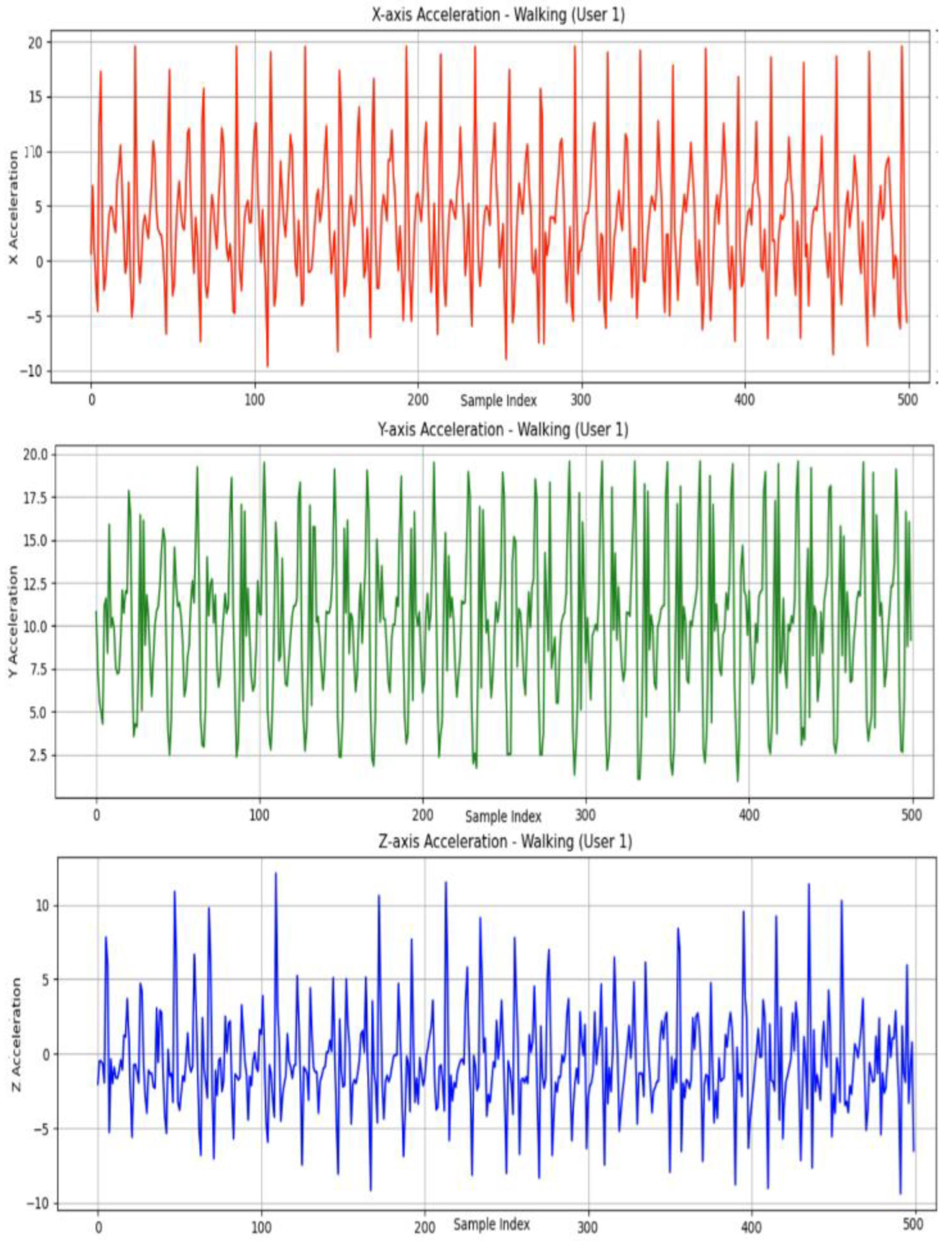
Figure 2.
Overview of the proposed HAR methodology.
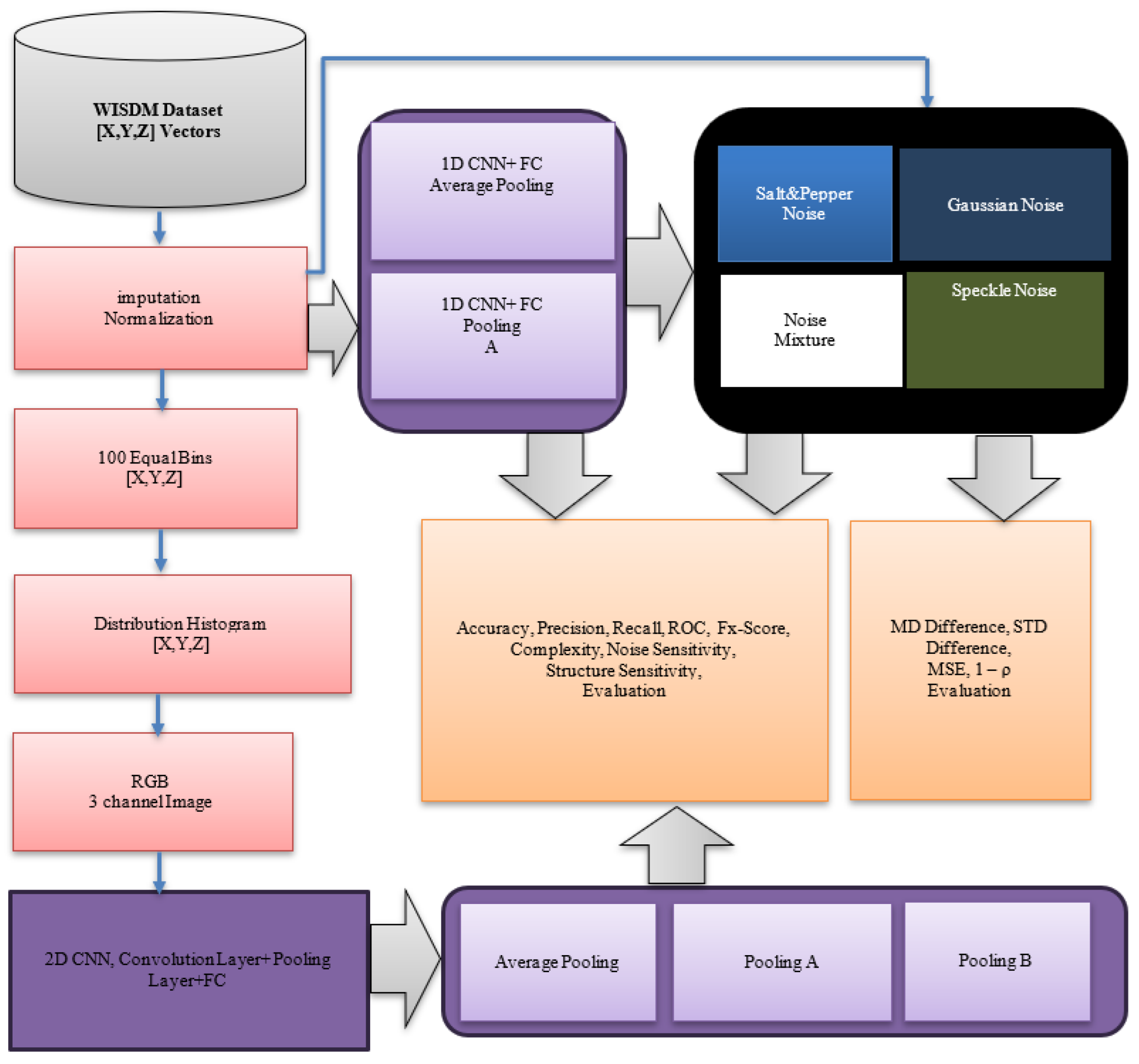
Figure 3.
STFT Spectrogram Comparison of Pooling Strategies on a Walking Activity Window.
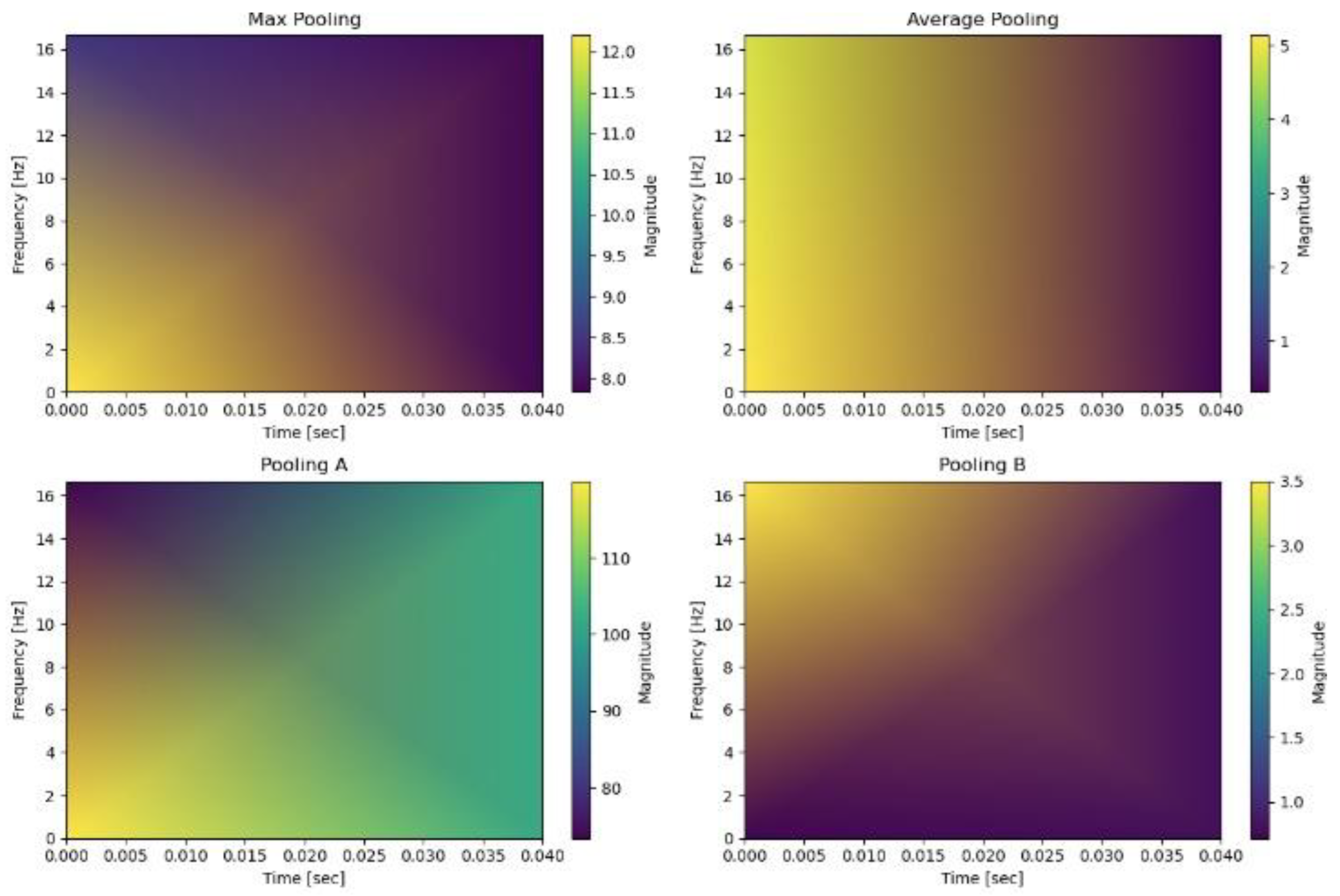
Figure 4.
Quantitative Comparison of Pooling Methods Under Various Noise Types (Mixture of all noise types) Using MD, STD, MSE, and 1−Correlation Metrics.
Figure 4.
Quantitative Comparison of Pooling Methods Under Various Noise Types (Mixture of all noise types) Using MD, STD, MSE, and 1−Correlation Metrics.
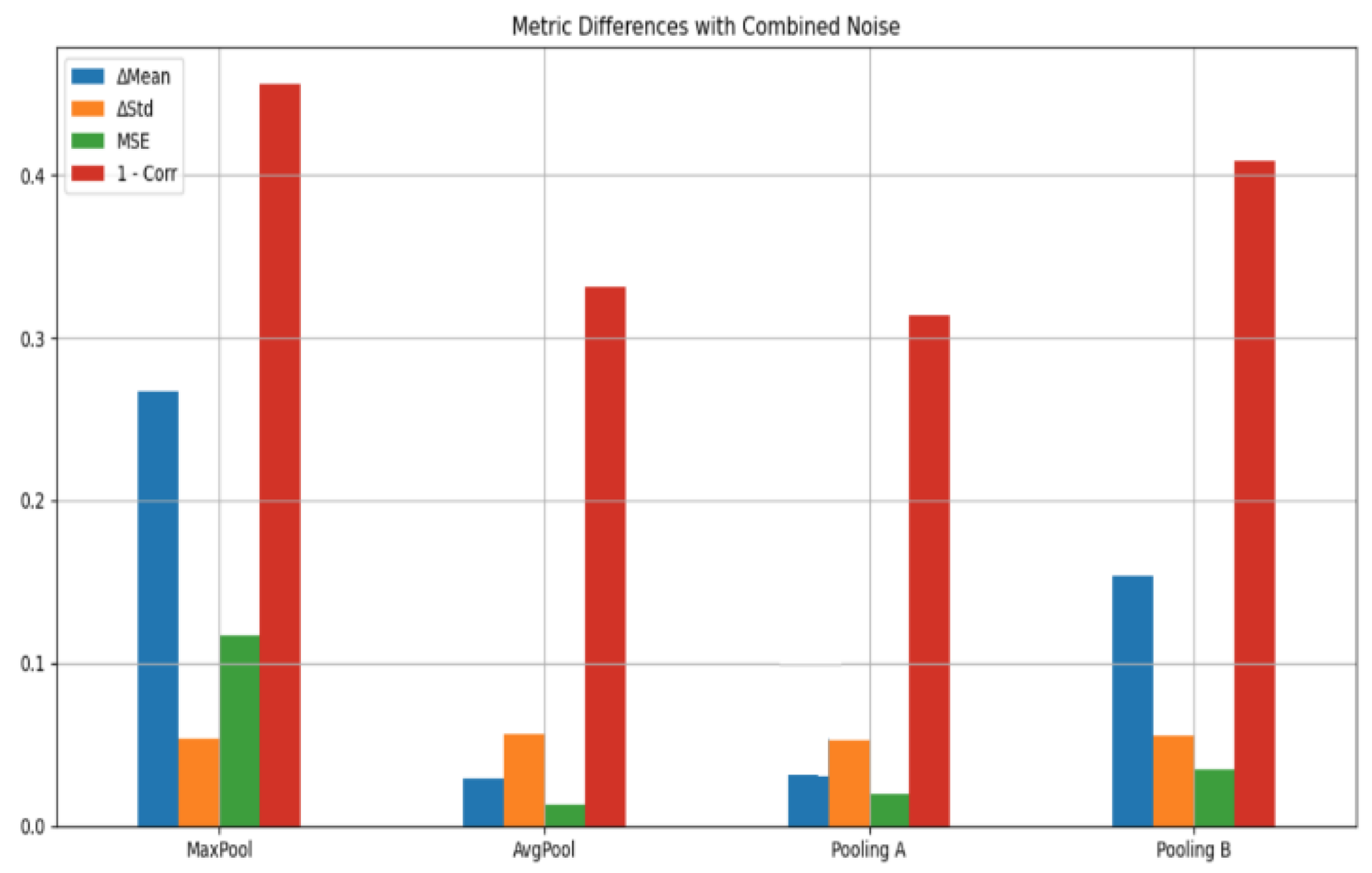
Figure 5.
Quantitative Comparison of Pooling Methods Under Various Noise Types (a) No noise, b) Under Gaussian noise, c) Under Salt&Pepper noise d) Under Speckle noise) Using MD, STD, MSE, and 1−Correlation Metrics.
Figure 5.
Quantitative Comparison of Pooling Methods Under Various Noise Types (a) No noise, b) Under Gaussian noise, c) Under Salt&Pepper noise d) Under Speckle noise) Using MD, STD, MSE, and 1−Correlation Metrics.
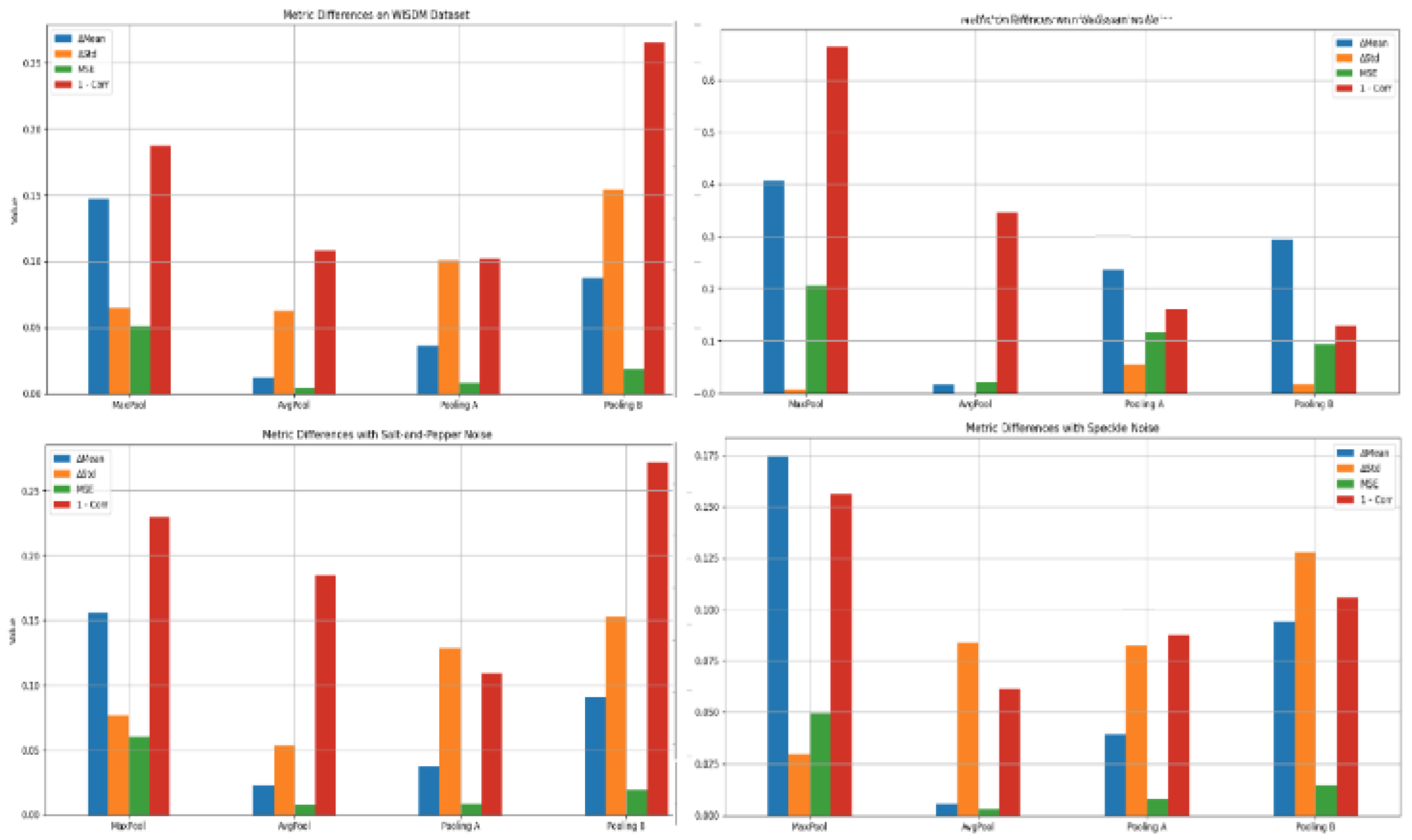
Figure 6.
STFT under Device Displacement Drift.
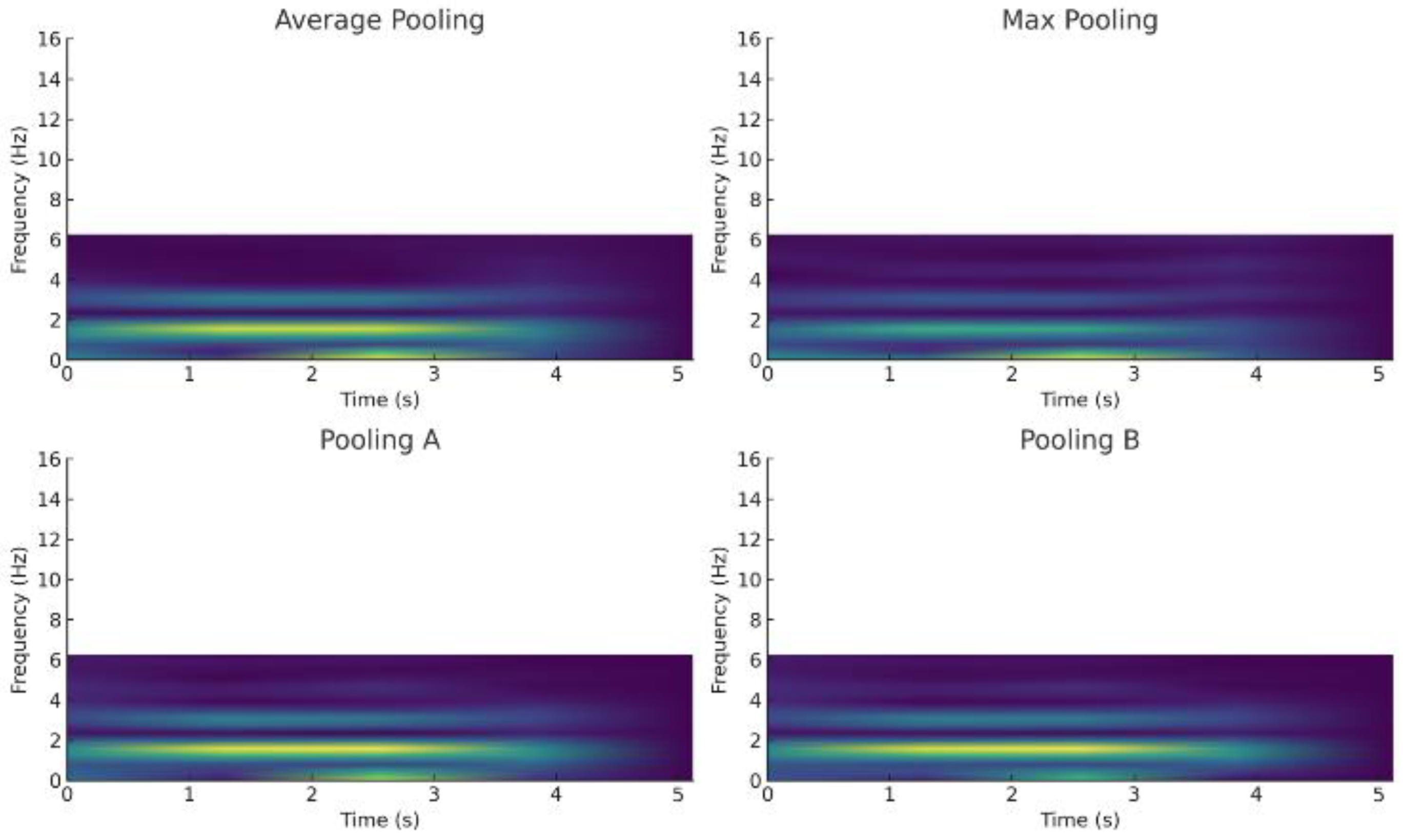
Figure 7.
X, Y and Z distributions.
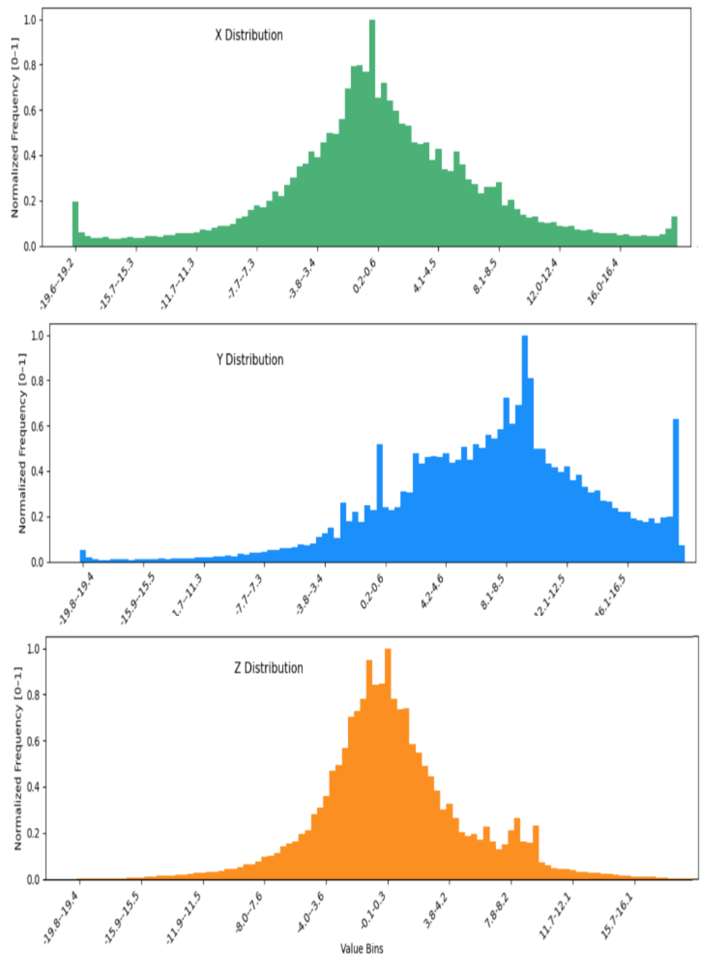
Figure 8.
Histogram distributions of X, Y, and Z accelerometer axes and the corresponding RGB-encoded image (Bin=100).
Figure 8.
Histogram distributions of X, Y, and Z accelerometer axes and the corresponding RGB-encoded image (Bin=100).
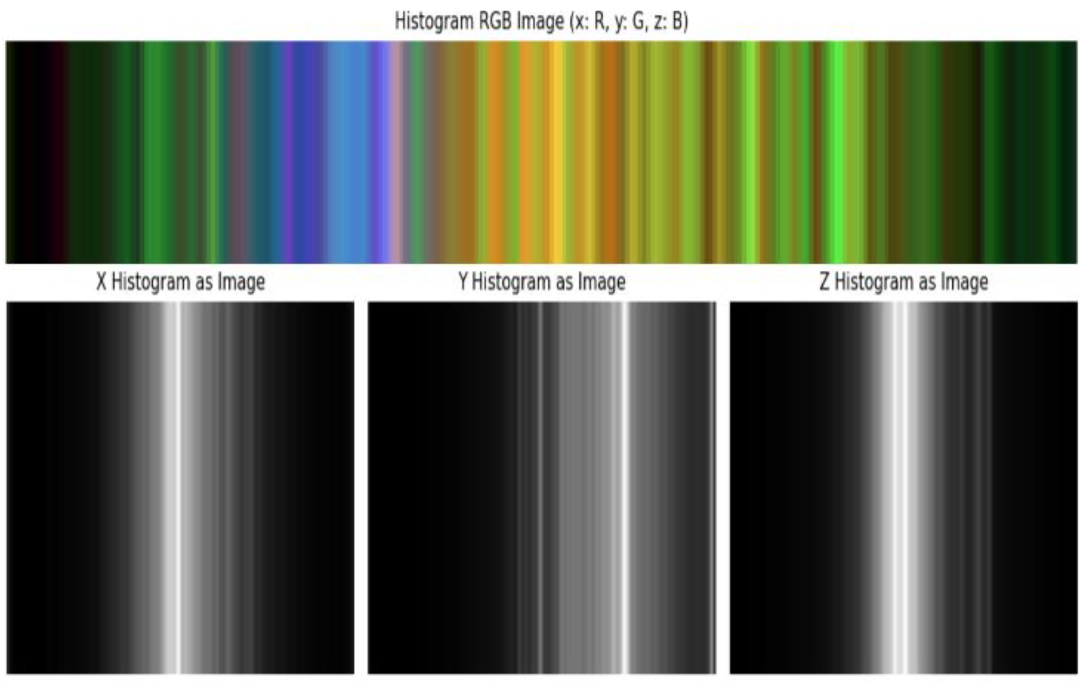

Table 1.
Technical Specifications.
| Parameter | Description |
|---|---|
| Device Used | Android smartphone with built-in accelerometer |
| Sampling Rate | ~20 Hz |
| Axes Captured | x, y, z |
| Number of Subjects | 36 |
| Activities Labeled | 6 (as listed above) |
| Windowing Scheme | 10-second non-overlapping segments (2-second overlapping for 10-second windows) |
| Label Granularity | Per window (not per sample) |
| Data Format | CSV: user, activity, timestamp, x, y, z |
Table 2.
User-activity frequency table from the WISDM dataset.
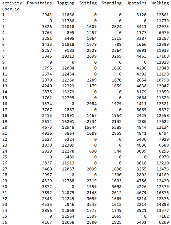
Table 3.
Cumulative statistics regarding dataset.
| Activity | Total Samples |
|---|---|
| Walking | 398,795 |
| Jogging | 340,511 |
| Upstairs | 121,168 |
| Downstairs | 100,269 |
| Sitting | 69,072 |
| Standing | 50,481 |
Table 4.
Transposed metrics comparison – 1D CNN with Pooling A vs. Average Pooling (all inputs min–max normalized to [0,1] to satisfy pooling constraints).
Table 4.
Transposed metrics comparison – 1D CNN with Pooling A vs. Average Pooling (all inputs min–max normalized to [0,1] to satisfy pooling constraints).
| Class | Precision (Avg) | Precision (A) | Recall (Avg) | Recall (A) | F1 Score (Avg) | F1 Score (A) | F2 (Avg) | F2 (A) | F0.5 (Avg) | F0.5 (A) | Support |
| Downstairs | 0.82 | 0.87 | 0.76 | 0.85 | 0.79 | 0.86 | 0.77 | 0.85 | 0.81 | 0.87 | 402 |
| Jogging | 0.98 | 0.95 | 0.98 | 0.96 | 0.98 | 0.96 | 0.98 | 0.96 | 0.98 | 0.96 | 1369 |
| Sitting | 0.97 | 0.98 | 0.96 | 0.98 | 0.97 | 0.98 | 0.96 | 0.98 | 0.97 | 0.98 | 239 |
| Standing | 0.99 | 1.00 | 0.99 | 0.99 | 0.99 | 1.00 | 0.99 | 0.99 | 0.99 | 1.00 | 193 |
| Upstairs | 0.79 | 0.92 | 0.92 | 0.96 | 0.85 | 0.94 | 0.89 | 0.95 | 0.81 | 0.93 | 491 |
| Walking | 0.97 | 0.99 | 0.96 | 0.98 | 0.96 | 0.99 | 0.96 | 0.98 | 0.97 | 0.99 | 1697 |
| Macro Avg | 0.92 | 0.95 | 0.93 | 0.95 | 0.92 | 0.95 | 0.92 | 0.95 | 0.92 | 0.95 | 4391 |
| Weighted Avg | 0.95 | 0.96 | 0.94 | 0.95 | 0.94 | 0.96 | 0.94 | 0.95 | 0.95 | 0.96 | 4391 |
Table 5.
Main Metrics Comparison – 1D CNN with Pooling A vs. Average Pooling.
| Metric/Class | Pooling A | Average Pooling | Preferred Approach |
|---|---|---|---|
| Accuracy(WeightedAvg) | 95.1% | 94.7% | Pooling A (slight improvement) |
| F1 Score (Downstairs) | 0.86 | 0.79 | Pooling A |
| F1 Score (Upstairs) | 0.96 | 0.87 | Pooling A (clear margin) |
| Recall (Upstairs) | 0.96 | 0.87 | Pooling A |
| Precision (Upstairs) | 0.95 | 0.86 | Pooling A |
| F1 Score (Jogging) | 0.96 | 0.98 | Average Pooling (slightly better) |
| ROC (Macro Average) | 0.97 | 0.95 | Pooling A |
| Computational Cost | Moderate | Low | Avg Pooling |
| Sensitivity to Noise | Low | Low | Pooling A |
| Sensitivity to Edges | Strong | Weak | Pooling A |
Table 6.
Salt-and-Pepper Noise Profiles Used in Experiments To ensure reproducibility.
| Noise Density (amount) | Description | Example in Python (skimage.util.random_noise) |
|---|---|---|
| 0.10 (10%) | Light corruption; ~1 in 10 samples replaced | random_noise(x, mode=‘s&p’, amount=0.10) |
| 0.20 (20%) | Moderate corruption; affects local features | random_noise(x, mode=‘s&p’, amount=0.20) |
| 0.30 (30%) | Heavy corruption; severe loss of fine detail | random_noise(x, mode=‘s&p’, amount=0.30) |
Table 8.
Signal deviation metrics under 20% noise for different pooling methods.
| Noise Type | Pooling | MD ↓ | STD ↓ | MSE | 1 − ρ |
|---|---|---|---|---|---|
| Salt & Pepper | Max Pooling | 0.16 | 0.07 | 0.05 | 0.23 |
| Average Pooling | 0.02 | 0.05 | 0.01 | 0.18 | |
| Pooling A | 0.03 | 0.13 | 0.01 | 0.11 | |
| Pooling B | 0.09 | 0.15 | 0.02 | 0.27 | |
| Gaussian | Max Pooling | 0.41 | 0.01 | 0.22 | 0.70 |
| Average Pooling | 0.01 | 0.00 | 0.02 | 0.33 | |
| Pooling A | 0.22 | 0.05 | 0.12 | 0.15 | |
| Pooling B | 0.29 | 0.02 | 0.09 | 0.12 | |
| Speckle | Max Pooling | 0.17 | 0.03 | 0.05 | 0.16 |
| Average Pooling | 0.02 | 0.08 | 0.01 | 0.06 | |
| Pooling A | 0.03 | 0.08 | 0.02 | 0.08 | |
| Pooling B | 0.09 | 0.13 | 0.04 | 0.10 | |
| Mixture Noise | Max Pooling | 0.27 | 0.06 | 0.11 | 0.445 |
| Average Pooling | 0.04 | 0.06 | 0.01 | 0.206 |
Note: indicates that lower is better. Best values per noise type are bolded.
Table 9.
Noise Robustness Evaluation summarization.
| Noise Type | Best Metric (per pooling) | Worst Performing |
|---|---|---|
| Salt & Pepper | Pooling A shows the lowest MSE and highest correlation; Average Pooling is competitive. | Max Pooling |
| Gaussian | Pooling A achieves best 1 − ρ; Average Pooling slightly better in MD, STD, and MSE; Pooling B performs closely to A. | Max Pooling |
| Speckle | Average Pooling performs best across all metrics; Pooling A remains a close second. | Max Pooling |
| Mixture Noise | Pooling A achieves better 1 − ρ; Average Pooling slightly better in MSE and MD. | Max Pooling |
| No Noise | Pooling A shows best 1 − ρ; Average Pooling marginally better in MSE and STD. | Max Pooling |
Table 10.
class-wise performance under clean and Gaussian noise conditions.
| True Class | Predicted (Clean) – Top Confusion | Predicted (Gaussian Noise σ=0.2) – Top Confusion | Comment |
|---|---|---|---|
| Walking | 96% Walking (4% Jogging) | 80% Walking (17% Jogging, 3% Standing) | Misclassified mainly as Jogging under noise |
| Jogging | 96% Jogging (4% Walking) | 78% Jogging (19% Walking, 3% Upstairs) | Overlaps with Walking under noise |
| Sitting | 98% Sitting (2% Standing) | 97% Sitting (3% Standing) | Robust to Gaussian noise |
| Standing | 98% Standing (2% Sitting) | 95% Standing (5% Sitting) | Slight degradation |
| Upstairs | 96% Upstairs (4% Downstairs) | 81% Upstairs (14% Downstairs, 5% Jogging) | Degraded, confuses with Downstairs |
| Downstairs | 94% Downstairs (6% Upstairs) | 82% Downstairs (16% Upstairs, 2% Jogging) | Degraded, confuses with Upstairs |
Table 11.
Latency and Computational Cost of Pooling Strategies for Edge Deployment.
| Pooling Type | Latency per Window (ms) | FLOPs Estimate | Deployable on Edge? |
|---|---|---|---|
| Average Pooling | 0.05 | Low | Yes |
| Max Pooling | 0.06 | Low | Yes |
| Pooling A | 0.08 | Moderate | Yes |
| Pooling B | 0.15 | Higher | Possibly* |
* Pooling B remains feasible for moderate HAR sampling rates, but its increased latency should be considered in real-time systems.
Table 12.
Precision, recall, and F1-score per class for histogram-based CNN+FC models.
| Metric/Method | Downstairs | Jogging | Sitting | Standing | Upstairs | Walking | Weighted Avg |
|---|---|---|---|---|---|---|---|
| Precision | |||||||
| Avg Pooling | 0.81 | 0.98 | 0.97 | 0.98 | 0.88 | 0.95 | 0.94 |
| Proposed Pooling A | 0.88 | 0.99 | 0.97 | 1.00 | 0.87 | 0.96 | 0.96 |
| Proposed Pooling B | 0.87 | 0.98 | 0.99 | 0.97 | 0.80 | 0.95 | 0.94 |
| Recall | |||||||
| Avg Pooling | 0.78 | 0.98 | 0.97 | 0.98 | 0.88 | 0.95 | 0.93 |
| Proposed Pooling A | 0.88 | 0.99 | 0.97 | 1.00 | 0.87 | 0.96 | 0.96 |
| Proposed Pooling B | 0.87 | 0.98 | 0.99 | 0.97 | 0.80 | 0.95 | 0.94 |
| F1 Score | |||||||
| Avg Pooling | 0.79 | 0.98 | 0.97 | 0.98 | 0.88 | 0.95 | 0.93 |
| Proposed Pooling A | 0.88 | 0.99 | 0.97 | 1.00 | 0.87 | 0.96 | 0.96 |
| Proposed Pooling B | 0.87 | 0.98 | 0.99 | 0.97 | 0.80 | 0.95 | 0.94 |
Table 13.
Quantitative and qualitative evaluation of various pooling techniques.
| Metric/Class | Proposed Pooling A | Proposed Pooling B | Average Pooling | Preferred Approach | |
|---|---|---|---|---|---|
| Accuracy (Weighted Avg) | 96.5% | 93.3% | 93% | Pooling A (highest accuracy) | |
| F1 Score (Downstairs) | 0.89 | 0.85 | 0.79 | Pooling A | |
| F1 Score (Upstairs) | 0.87 | 0.80 | 0.88 | Average Pooling (slightly higher F1) | |
| Recall (Upstairs) | 0.87 | 0.80 | 0.88 | Average Pooling | |
| Precision (Upstairs) | 0.87 | 0.80 | 0.88 | Average Pooling | |
| F1 Score (Jogging) | 0.99 | 0.97 | 0.97 | Pooling A(highest) | |
| F1 Score (Sitting) | 0.97 | 0.99 | 0.96 | Pooling B (slightly better) |
|
| F1 Score (Standing) | 1.00 | 0.96 | 0.97 | Pooling A | |
| F1 Score (Walking) | 0.96 | 0.94 | 0.94 | Pooling A | |
| ROC (weighted Average) | 0.98 | 0.93 | 0.94 | Pooling A | |
| Computational Cost | Moderate | Moderate | Low | Average Pooling | |
| Sensitivity to Noise | Low | Moderate | Low | Pooling A / Avg | |
| Sensitivity to Edges | Strong | Moderate | Weak | Pooling A | |
Table 14.
Effect of Histogram Bin Size.
| Input Representation | Bin Size | Accuracy (%) | Macro F1 | Weighted F1 | Remarks |
|---|---|---|---|---|---|
| Histogram Encoding | 50 | 93.8 | 0.93 | 0.94 | Coarse bins, lower resolution |
| Histogram Encoding | 100 | 95.0 | 0.95 | 0.95 | Balanced trade-off |
| Histogram Encoding | 200 | 95.1 | 0.95 | 0.95 | Slight gain, higher cost |
| Raw Window (2D CNN) | – | 92.6 | 0.92 | 0.92 | Transformation ablated |
Table 15.
Class-wise Performance on Overlapping Sliding Windows (Stride = 50% of Window Size).
| Activity | Precision | Recall | F1 Score | Comparison vs. Non-overlapping (20%) |
|---|---|---|---|---|
| Downstairs | 0.82 | 0.80 | 0.81 | −5 |
| Jogging | 0.96 | 0.95 | 0.95 | −1 |
| Sitting | 0.97 | 0.97 | 0.97 | −1 |
| Standing | 0.98 | 0.97 | 0.97 | −3 |
| Upstairs | 0.88 | 0.85 | 0.86 | −8 |
| Walking | 0.96 | 0.95 | 0.95 | −4 |
| Macro Avg | 0.93 | 0.91 | 0.92 | −4 |
| Weighted Avg | 0.94 | 0.92 | 0.93 | −3 |
Table 16.
False Positive Rates under Motion Artifact Perturbations.
| Activity (True Label) | Noise-Free Accuracy (%) | With Motion Artifact (Avg. Shaking Amplitude 0.5g) | False Positive Rate (%) | Most Frequent Misclassification |
|---|---|---|---|---|
| Standing | 99.8 | 92.1 | 7.9 | Walking |
| Sitting | 98.9 | 90.7 | 8.2 | Standing |
| Walking | 96.7 | 91.4 | 5.3 | Jogging |
| Jogging | 95.2 | 91.9 | 3.3 | Walking |
| Upstairs | 93.5 | 86.4 | 7.1 | Downstairs |
| Downstairs | 92.7 | 85.5 | 7.2 | Upstairs |
Table 17.
Per-class accuracy (%) across models and pooling strategies.
| Histogram-aware CNN+FC (Average Pooling) | Histogram-aware CNN+FC (Proposed Pooling A) |
Histogram-aware CNN+FC (Proposed Pooling B) |
1D CNN (Average Pooling) |
1D CNN (Pooling A) |
|
|---|---|---|---|---|---|
| Downstairs | 78.3 | 87.8 | 87.3 | 78.8 | 85.8 |
| Jogging | 98.2 | 98.9 | 98.1 | 98.3 | 95.6 |
| Sitting | 97.0 | 97.4 | 98.7 | 97.0 | 97.9 |
| Standing | 98.1 | 100 | 97.0 | 98.9 | 99.4 |
| upstairs | 88.3 | 86.5 | 80.0 | 87.3 | 95.8 |
| Walking | 95.0 | 96.1 | 95.4 | 95.3 | 98.3 |
| weighted Average | 93.0 | 96.5 | 93.3 | 94.7 | 95.3 |
Table 18.
A qualitative comparison of the proposed method with several existing approaches.
| Study | Dataset Used | Model Type | Feature Representation | Pooling Strategy | Noise Robustness | Reported Accuracy (%) | Remarks |
|---|---|---|---|---|---|---|---|
| Kwapisz et al. (2011) [ACM SigKDD] [1] | Original WISDM v1.0 | Multilayer Perceptron (MLP) | Handcrafted features (mean, std, etc.) | N/A | Not addressed | ~91.7 | Classical benchmark; no deep learning used |
| Walse et al. (2016) [ICTCS] [2] | WISDM v1.0 | k-NN, J48, Random Forest | Manual statistical features | N/A | Not addressed | ~84–89 | Focus on classical ML classifiers |
| Min et al. (2020) [IJC] [3] | WISDM v1.0 | SVM, RF, KNN | Time-domain features | N/A | Not addressed | ~90.2 (best) | No deep architectures; limited generalization |
| Seelwal & Srinivas (2023) [JOEE] [4] | WISDM v1.1 | CNN | Raw time-series input | Max pooling | Not addressed | 92.8 | Used basic CNN without preprocessing enhancements |
| Heydarian & Doyle (2023) [arXiv] [5] | rWISDM (Repaired WISDM) | CNN-LSTM Hybrid | Denoised signals | Max pooling | ✓ Basic denoising applied | 93.1 | Enhanced input via preprocessing, but no custom pooling |
| Sharen et al. (2024) [ESWA] [6] | WISDM v1.1 | WISNet (Custom DNN) | Raw signals + domain features | Avg/Max pooling | Minimal robustness | 94.5 | Deep model, but no redundancy modeling or pooling innovation |
| Abdellatef et al. (2025) [Sci. Reports] [7] | WISDM v1.1 | Multi-layer CNN | Raw time-series | Avg pooling | Not addressed | 94.2 | Strong architecture but lacks input transformations |
| This Work (2025) | Based on WISDM | Dual-path: 1D CNN + Histogram-aware 2D CNN | Raw time-series + Histogram-to-RGB image | Proposed Pooling A & B | ✓ Robust to Gaussian, S&P, Mixed noise | 96.5 | First to combine redundancy modeling + pooling design for noise-aware HAR |
Table 19.
Cross-Dataset Results (Proposed vs. Baselines).
| Dataset | Model/Pooling | Accuracy (%) | Macro F1 | Notes | |
|---|---|---|---|---|---|
| WISDM | Proposed (Pooling A) | 96.5 | 0.95 | Our main benchmark, segmentation-based windows | |
| UCI-HAR | Proposed (Pooling A) | 95.2 | 0.94 | Slightly below SOTA (>97%), confirms transferability | |
| MobiAct | Proposed (Pooling A) | 94.7 | 0.93 | Generalizes but drops in activities with high inter-user variability | |
| WISDM | Average Pooling (CNN) | 94.7 | 0.92 | Baseline comparison | |
Disclaimer/Publisher’s Note: The statements, opinions and data contained in all publications are solely those of the individual author(s) and contributor(s) and not of MDPI and/or the editor(s). MDPI and/or the editor(s) disclaim responsibility for any injury to people or property resulting from any ideas, methods, instructions or products referred to in the content. |
© 2025 by the authors. Licensee MDPI, Basel, Switzerland. This article is an open access article distributed under the terms and conditions of the Creative Commons Attribution (CC BY) license (http://creativecommons.org/licenses/by/4.0/).
Copyright: This open access article is published under a Creative Commons CC BY 4.0 license, which permit the free download, distribution, and reuse, provided that the author and preprint are cited in any reuse.


