
Submitted:
19 November 2025
Posted:
20 November 2025
You are already at the latest version
Abstract
Airborne particulate emissions originating from bulk-material handling operations constitute an increasingly critical environmental and public health issue in port-industrial areas located near residential areas. This study introduces a novel hybrid framework integrating high-fidelity Computational Fluid Dynamics (CFD) with surrogate Machine Learning (ML) techniques for the rapid assessment of particle dispersion in port-industrial environments. Focusing on the Port of El Grao in Castellón de la Plana (Spain), the study employs detailed geometric reconstructions derived from LiDAR data and cadastral maps to build an accurate three-dimensional digital model of the area. The turbulent atmospheric boundary layer and particle dispersion dynamics were simulated using two different OpenFOAM solvers within a circular computational domain designed to reproduce realistic wind conditions. The ML surrogate model, based on a decoder-style Multilayer Perceptron (MLP) architecture, processes two-dimensional slices of dispersion fields across particle diameter classes, enabling predictions in milliseconds with an acceleration factor of approximately 8×10⁶ over traditional CFD while preserving high fidelity, as validated by error metrics such as the F1 score and Precision values exceeding 0.8 and 0.76 respectively. This approach not only addresses computational inefficiencies but also lays the groundwork for real-time air quality monitoring and sustainable urban planning, potentially integrating with digital twins fed by live weather data.
Keywords:
machine learning
; CFD
; OpenFOAM
; particulate matter
; port areas
1. Introduction
Ports are recognized as significant contributors to urban air pollution where dry bulk commodities (e.g., mineral concentrates, clinker, coal, gypsum, and grains) are handled at the land–sea interface. Regional syntheses and city-scale assessments show that port-related sources—including vessel traffic, cargo handling, and heavy-duty road traffic—can materially affect ambient particulate matter (PM) across size fractions, adding mineral dust and trace metals to the urban background, particularly under dry and windy conditions typical of many Mediterranean and Atlantic harbors [62,64,65]. In Alicante (western Mediterranean), source apportionment at the port–city boundary attributed 35% of average PM10 to bulk-handling factors (limestone, gypsum, and clinker), compared with 6% from shipping emissions, highlighting the importance of terminal operations for near-field exposure [56]. These findings are consistent with broader European evidence that shipping contributes variably to PM mass but disproportionately to particle number and ultrafine particles (UFP), with port plumes impacting inland areas under sea-breeze fumigation [57,59,65]. Policy frameworks in Spain and across the EU increasingly embed air-quality obligations into port governance and industrial permitting, facilitating the adoption of best available techniques, shore power, and dust-management measures. However, even ambitious mitigation scenarios suggest that local source control remains critically important, particularly for UFP, which are not fully addressed by mass-based standards. Taken together, this literature positions bulk-handling operations as critical intervention points for reducing population exposure in port–city settings.
In recent years, European and Spanish air-quality regulations have become increasingly stringent, especially regarding concentrations of suspended particulate matter. The updated EU Directive for ambient air quality sets substantially lower limit values for PM10 and PM2.5 to be achieved by 2030, reflecting growing evidence of their adverse health effects. Additionally, the revision of occupational exposure limits under Directive (EU) 2017/2398 explicitly restricts exposure to respirable crystalline silica, a pollutant frequently associated with bulk-material handling in port environments. These regulatory developments impose stronger monitoring requirements and demand more accurate tools for identifying emission sources and predicting their impact on surrounding communities.
Despite the presence of regulatory frameworks such as the Spanish Ley 34/2007 on air quality and atmospheric protection, compliance mechanisms in port–industrial environments remain hampered by the limited resolution of current monitoring strategies. Fixed sensor networks provide only discrete, point-based measurements and do not meet the level of spatial and temporal detail required to understand short-duration peak events, which are precisely the episodes most relevant for regulatory exceedances. Furthermore, dispersion tools commonly used for environmental impact assessments—primarily Gaussian models—are not designed to resolve near-field urban aerodynamics and therefore cannot reliably support regulatory diagnostics in complex port–city interfaces where exceedances often occur. This methodological gap compromises the ability of port authorities and industrial operators to anticipate non-compliance situations and to deploy targeted mitigation measures.
Within bulk logistics, loading and unloading of trucks are recurrent, high-intensity PM sources with complex spatiotemporal behavior. Dust is generated during tipping, hopper discharge, and transfers, where gravitational fall, impact, and induced turbulence entrain fines; subsequent truck accelerations and braking on silt-laden pavements promote vigorous non-exhaust resuspension that can dominate short-term peaks at yards and port–city boundaries, especially under unfavorable meteorology [55,56,60]. Downwind of mineral bulk terminals, trace-metal fingerprints in deposited dust and soils (e.g., Pb, Ni, Cd, As) corroborate a port signature in urban areas, reinforcing the need for control at transfer points and truck loading bays [64]. Engineering controls—encapsulated or aspirated hoppers, covered conveyors or telescopic spouts, fog/mist cannons, targeted wetting of haul roads, and windbreaks—can deliver substantial but context-dependent reductions; for example, controlled experiments over ore piles show mist generators can reduce PM10 by ∼70–80% under favorable operating parameters, while road-dust management reduces non-exhaust contributions but requires sustained maintenance and meteorology-aware operation [55,60,61]. At the worker scale, grain loading into holds and hoppers exposes stevedores to high dust and bioaerosol concentrations, adding an occupational dimension to control priorities [58]. Because emissions and exposure depend strongly on wind regimes, terminal geometry, materials, and the choice and placement of abatement technologies, port-specific diagnostic and prognostic tools are needed.
To address these challenges, advanced simulation techniques boosted by real-time data and high-performance computing have become indispensable for devising mitigation strategies and supporting sustainable planning at the urban–port interface [16]. Computational Fluid Dynamics (CFD) provides a robust framework for resolving airflow and pollutant dispersion in complex geometries, capturing the effects of buildings, terminal infrastructure, and local roughness on turbulent transport [20,25]. In parallel, the rapid evolution of Industry 4.0 and smart-city paradigms is driving the integration of CFD with Machine Learning (ML) to build surrogate models capable of emulating high-fidelity simulations at a fraction of their computational cost [23,24]. Recent studies have demonstrated that deep learning architectures—including three-dimensional convolutional neural networks, residual neural networks, and physics-informed neural networks—can reproduce key flow and dispersion features while achieving orders-of-magnitude acceleration [1,2,11,12,15,21,22,26,28]. These advances pave the way for near-real-time environmental diagnostics, scenario exploration, and decision support in urban air-quality management [5,6,7,8,9,10].
Nevertheless, traditional CFD remains computationally expensive for routine or real-time applications, and existing CFD–ML hybrids often lack a specific focus on particulate emissions from port bulk terminals. In particular, there is limited work on (i) digital twins that integrate high-resolution geometric reconstructions of port infrastructure with (ii) particle-resolved dispersion simulations and (iii) surrogate models optimized for millisecond-scale inference over meteorological and operational scenarios relevant to regulatory diagnostics [6,10,28]. Data scarcity for robust training and the absence of standardized, end-to-end workflows further constrain operational deployment in real port–city environments.
Bulk-material handling operations—such as truck loading, unloading, and on-site stockpiling—are therefore a priority application for hybrid CFD–ML approaches. In the Port of El Grao (Castellón de la Plana, Spain), the materials most frequently handled include ceramic raw materials (such as clays, feldspars, and kaolin), mineral powders, and petroleum coke, all characterized by broad granulometric distributions with a significant fraction of respirable particles below 10 m and, in certain cases, containing crystalline silica. Their low moisture content and high friability increase their propensity to become airborne under moderate wind speeds, while their density and irregular morphology influence their settling behavior and potential for long-range transport. These physicochemical properties, combined with the operational dynamics of bulk handling, make these materials particularly relevant for studying particulate dispersion and assessing potential exposure in adjacent urban areas. Under certain meteorological conditions, the resulting particulate plumes can be transported toward nearby residential areas, posing an environmental and public-health concern.
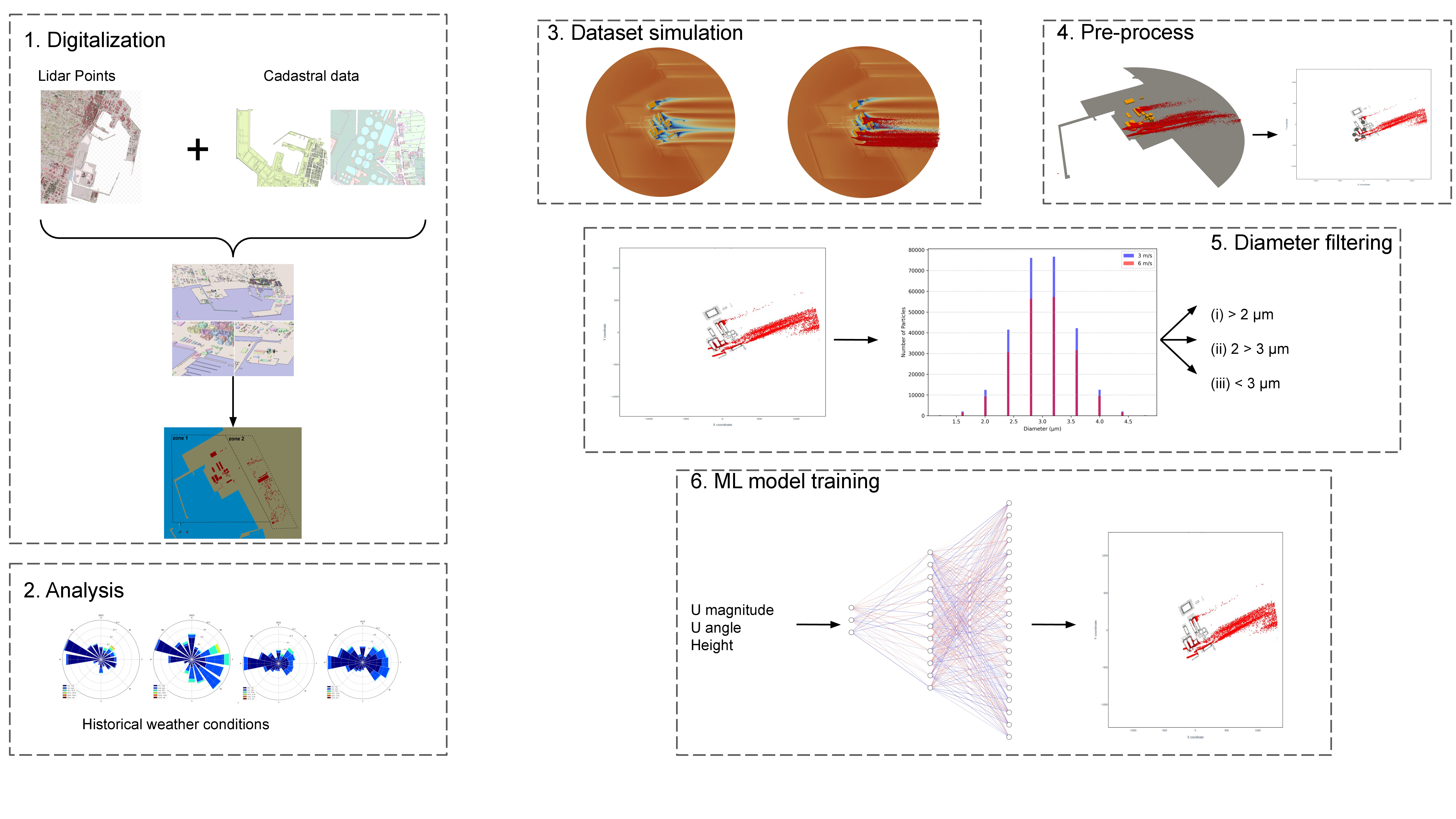
To address this issue, the present work introduces a hybrid approach that integrates high-fidelity CFD with surrogate ML techniques to evaluate particle dispersion in a port-industrial environment with nearby population exposure. The methodology provides substantial computational acceleration while preserving the physical fidelity necessary for environmental impact assessment. The key contributions of this study are:
- Port-Industrial Digitalization and Mesh Generation: A high-resolution 3D digital model of the Port of El Grao (Castellón de la Plana, Spain) was developed using LiDAR data, cadastral information, and CAD processing, enabling a geometrically accurate representation of port infrastructure.
- Integrated CFD–ML Workflow: A workflow combining OpenFOAM-based aerodynamic and particulate transport simulations with a decoder-style ML model architecture is proposed. Horizontal (Z-axis) 2D slices of the particle concentration fields are used to train the surrogate model, with hyperparameters optimized using Optuna framework for efficient convergence.
- Performance and Accuracy: While CFD simulations required 432,000 s for steady state and 108,000 s for transient state on 100 cores, the trained ML surrogate performed inference in milliseconds on a GPU, achieving a computational acceleration factor of approximately . Validation results demonstrate that the ML model reliably reproduces CFD predictions across multiple wind scenarios.
The rest of the paper is organized as follows. Section 2 describes the methodology employed in this study, from the CFD set-up to the ML model design and training. Section 3 presents the results, organized into three subsections: aerodynamics, particle dispersion, and machine learning. Section 4 concludes the paper and discusses future work.
2. Methods
This section describes the methodology employed in the present study, which integrates multiple computational techniques to assess atmospheric particle dispersion.
The study focuses on the port–industrial district of El Grao in Castellón de la Plana (Spain), a densely integrated coastal environment where heavy industrial activity, residential neighbourhoods, and transport infrastructure coexist within a relatively compact area (Figure 1). The port hosts intensive bulk-material handling operations, including the loading, unloading and storage of mineral powders, ceramic raw materials and petcoke, all of which are prone to generating fine particulate emissions. These facilities are situated only a few hundred meters from urban residential zones, separated by a heterogeneous built environment composed of warehouses, breakwaters, medium-rise buildings, and open yards that shape complex wind-flow patterns. The proximity between industrial sources and populated areas, combined with the prevalence of onshore sea-breeze regimes characteristic of the western Mediterranean coast, frequently facilitates the transport of suspended particulate matter inland. This configuration makes El Grao an especially representative and challenging scenario for assessing air-quality impacts in port–city interfaces, highlighting the need for high-resolution modelling tools capable of reproducing the intricate aerodynamics and dispersion phenomena that govern exposure levels.
It should be noted that the modelization of the urban area is out of the scope of the current research. The overall approach comprises the following phases: Computational model, Computational domain and Boundary Conditions, Validation of the Aerodynamics, Data Pre-process and I/O Depiction and ML Model.
2.1. Computational Model
In CFD simulations of urban environments, turbulence modeling governs the balance between fidelity and computational cost. Direct Numerical Simulation (DNS) resolves all turbulent scales and offers the highest accuracy but is computationally infeasible for the very large Reynolds numbers typical of city domains (–) because it requires grids down to the Kolmogorov scale [41]. Large Eddy Simulation (LES) resolves the energy-containing eddies while modeling the subgrid scales, capturing unsteady, intermittent features of urban flows and street-canyon dispersion more faithfully than averaged approaches, but at costs that are often orders of magnitude higher—impractical for large parametric datasets across many wind scenarios [42,43,44]. By contrast, Reynolds-Averaged Navier–Stokes (RANS) models statistically average the equations and represent all turbulence via closures (e.g., k-), yielding a robust and computationally efficient option widely used in wind engineering [45].
In this study, CFD techniques were employed using OpenFOAM, an open-source CFD toolbox, to model particle dispersion under a neutral atmospheric boundary layer (ABL). The wind flow was resolved using the steady RANS equations with the k- turbulence model, owing to its validated performance in atmospheric dispersion modelling [35]. This choice enables the simulation of the multiple cases required for dataset construction while remaining feasible within the available computational resources.
For the wind flow, the steady-state, incompressible turbulent flow solver simpleFoam was used. This solver has been designed to solve RANS equations using the SIMPLE (Semi-Implicit Method for Pressure-Linked Equations) algorithm for pressure-velocity coupling.
The simulation of particle transport was carried out using the icoUncoupledKinematicParcelFoam solver in OpenFOAM, which is specifically designed for transient modeling of kinematic particle clouds advected by a precomputed flow field. The adopted methodology follows an Euler–Lagrangian approach, where the continuous phase (air) is first resolved using the simpleFoam solver under steady-state conditions with the k- turbulence model within the RANS framework to obtain a converged aerodynamic field. Subsequently, the discrete phase (particles) is tracked in time using one-way coupling, assuming negligible feedback on the carrier flow. The governing equations account for dominant forces such as drag, gravity, and pressure gradients, while neglecting inter-particle collisions due to low concentration. Boundary conditions include atmospheric boundary layer profiles at the inlet and specific wall interaction models (elastic rebound on terrain and buildings, adhesion on water surfaces). This two-step procedure enables a realistic assessment of particle dispersion in complex port environments, capturing the influence of obstacles and turbulence on transport dynamics.
2.2. Computational Domain and Boundary Conditions
To construct the geometry model of the study domain, LiDAR point clouds were obtained from the National Plan for Aerial Orthophotography (PNOA-LiDAR1) via the National Geographic Information Center (CNIG). This data was used for classifying the key features of the domain, including buildings, vegetation, and terrain. To further enhance the accuracy of the digital model, cadastral maps from the Spanish Cadastre and Mapping Agency2 were incorporated to provide detailed parcel and road boundaries.
The integrated processing yielded three raster digital models (DEM, DSM, nDSM) and two Geopackage layers containing both elevation and height data. A 3D polygonal model was then generated using ArcGIS Pro®, employing extrusion techniques based on the derived 3D values. Further refinements were accomplished in CAD software (e.g., Blender®) to optimize both the level of detail and computational efficiency (see Figure 2 for further information).
The final model obtained comprises three primary geometries: sea, terrain, and industrial buildings emitting particulate matter into the atmosphere. Figure 3 schematically depicts the computational domain used in this study. The domain height H is fixed at 130 m to fully encompass the ABL and prevent vertical interference, while the domain diameter D was fixed at 2600 m, following CFD best-practice guidelines and recommendations from [29,30,31].
Figure 3 also illustrates the boundary conditions applied in the simulations. To ensure a homogeneous neutral atmospheric wind profile in the horizontal plane, inflow conditions were implemented in OpenFOAM using the atmBoundaryLayer class [32] for streamwise wind velocity (U), turbulent kinetic energy (k), and turbulent dissipation rate (). In this context, atmBoundaryLayerInletVelocity boundary condition provides a log-law type inlet boundary condition for the flow speed profile expression:
with the following parameters: von Kármán constant (-) and aerodynamic roughness length () equal to 0.01 m for ground and 0.0002 m for sea according to the classification proposed by [54]. The friction velocity is given by:
where (m/s) is the reference streamwise wind speed at a reference height . To select the values, data from one of the meteorological stations located within the study area and closest to the inlet boundary of the computational domain were used (Figure 4a, P1). This station is located 14 m above the ground, a value that was therefore assigned to . The wind rose was generated using accumulated data from two consecutive years (2022-2023), (Figure 4.b). We selected the wind-direction angles whose trajectories advect particles toward the urban area (Figure 4.a, yellow-shaded sector). In this case, ∈ [130°-170°], corresponding to winds originating from the south–southeast sector.
To model the turbulent viscosity, wall function was applied to the ground and buildings surfaces using atmNutkWallFunction and nutkWallFunction respectively. As has been commented, the air flow aerodynamics distribution was resolved in the first step, Table 1 shows the boundary conditions imposed in the simulation. To improve the homogeneity of the velocity profile in the streamwise direction, a fixed shear stress boundary condition () was applied at the top boundary of the domain [34]. Table 1 presents a summary of all the boundary conditions applied.
The particulate phase in the simulations was modeled using physical properties representative of dust generated during bulk cargo handling. For the particle size distribution, the model assumes a normal distribution centered around a representative mean diameter of approximately 3 , which reflects the fine fraction typically generated during bulk cargo handling operations. Although initial analyses considered specific materials such as clay (2.84 ) and feldspar (3.86 ), the final approach opted for a simplified representation using an average particle size to reduce computational complexity while maintaining physical realism. The particle density was assumed to be 2,600 , consistent with silicate-based minerals. Interactions with surfaces were defined through restitution coefficients: elastic rebound on terrain and building walls (normal and tangential coefficients set to 0.97) and adhesion on water surfaces (coefficients set to zero). The particles were treated as passive tracers under a one-way coupling assumption, meaning they do not influence the carrier flow. Collisions between particles were neglected due to low concentration, and gravitational settling was included to account for deposition of larger particles. These assumptions allow for a realistic yet computationally efficient representation of particulate dispersion in port environments.
Figure 5 shows the location of the seven bulk-material handling operations modelled within the study area. To ensure computational tractability, the simulation employs a computational parcel concept. Instead of tracking every individual particle, each parcel represents a defined cluster of real particles that share identical properties (e.g., diameter, density). The solver computes the trajectory for the parcel, and the results are interpreted as the collective behavior of the particles it represents. The particle properties for each source are presented in Table 2.
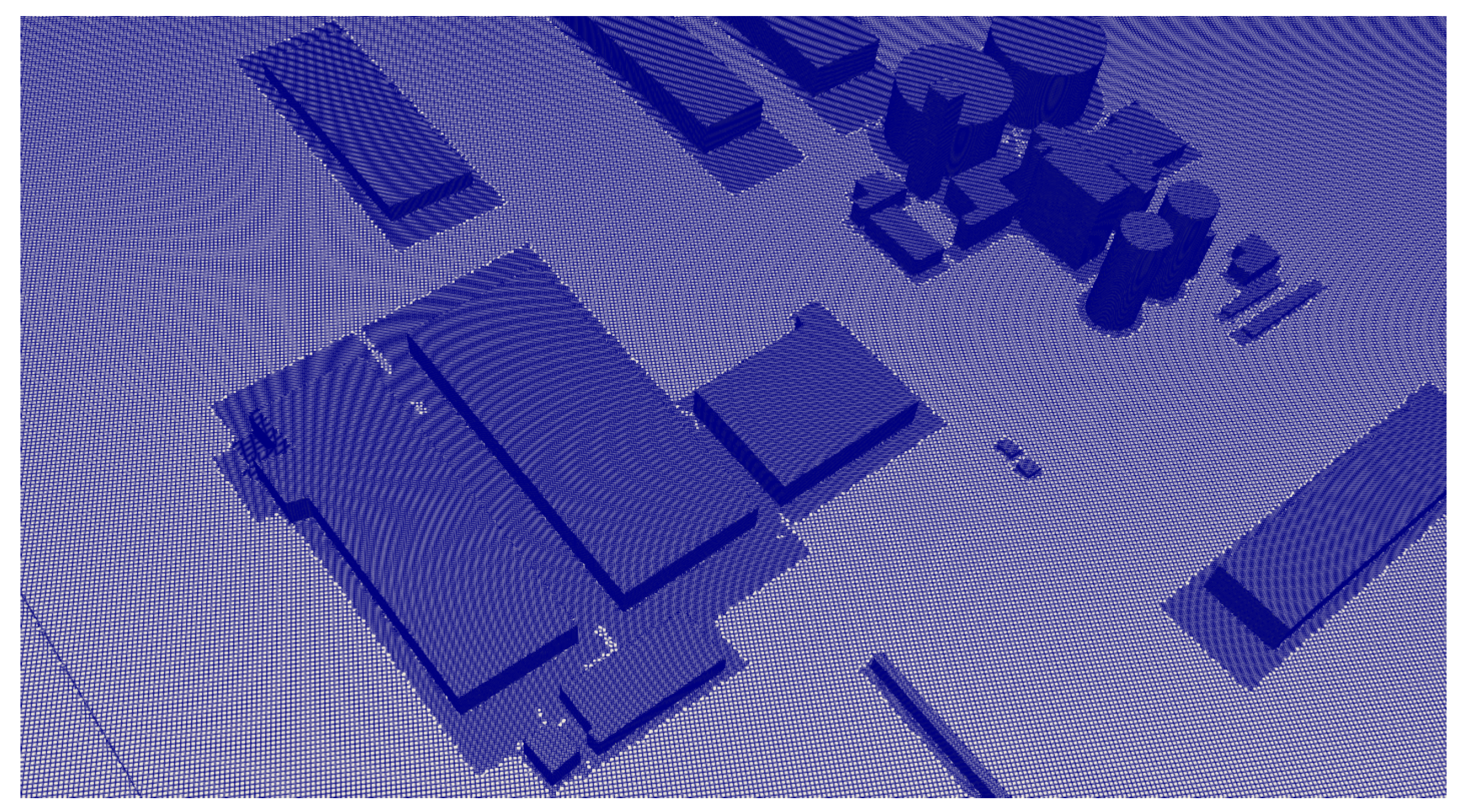
The computational domain was discretized using OpenFOAM’s blockMesh and snappyHexMesh utilities. Initially, the geometry was cleaned in Rhino 3D® to produce a watertight model, after which the surfaces were exported as STL files for subsequent mesh refinement. Although a rectangular domain was first attempted, its inability to maintain a consistent flow angle led to the adoption of a circular domain as presented in Figure 3.a. This configuration guarantees a uniform flow direction from inlet to outlet, eliminating edge and vertex effects such as local accelerations or artificial gradients. By segmenting the circumferential inlet-outlet face into multiple parts, the wind conditions for all angles can be defined within a single CAD and mesh file, with a dedicated script assigning the appropriate segments as inlets [36].
To achieve high resolution near walls, the snappyHexMesh algorithm was employed with a customized meshing strategy. The domain was partitioned into three refinement levels via volumetric control zones defined in a CAD program; the innermost zone, extending 1.5 m above the ground, received the highest refinement with additional layers for each building geometry. The optimized mesh comprised approximately 43 million cells within the circular domain, achieving an average y-plus value of 110 and ensuring reliable resolution of the urban wind environment. The minimum cubic edge length was 4.4 cm (due to local refinement) and the maximum cubic edge length was 9.3 m.
Figure 6.
Computational grid on the industrial buildings surfaces and part of the ground surface.
2.3. Validation of the Aerodynamics
For aerodynamic validation, data from the meteorological stations located within the study area (Figure 4.a) were used for the year 2022. Meteorological station P1 was designated as the reference station, as the inlet velocity profiles of the simulations, based on , were selected according to the analysis of the data from this station. Conversely, meteorological station P2 was established as the validation station, since it lies within the simulated computational domain but is not in close proximity to the reference station (approximately 1 km away).
Figure 7 shows the complete 2022 year wind data (speed and direction) from both stations. As observed, the temporal evolution of wind speed and direction exhibits a correlated trend at both sites, despite the approximately 1 km separation between them, indicating that both stations experience comparable atmospheric forcing.
The simulation used for validation was performed with inlet conditions of =2 m/s and =150º. The corresponding wind velocities at the locations of the two stations (averaged over the nodes adjacent to their exact positions) are presented in Table 3.
Based on the inlet wind boundary conditions of the simulation, the corresponding velocity and direction values were selected at the reference station (P1), considering an uncertainty of 10% in both parameters. Subsequently, the corresponding velocity and direction values were also selected at the validation station (P2). Validation was performed by comparing the velocity values obtained at station P1, selected for the same hourly intervals corresponding to station P2 (Figure 8). The results indicate that the average velocity values measured at the validation station and those obtained from the CFD simulation exhibit reasonable agreement for the presented case study.
2.4. Data Pre-Process and I/O Depiction
To create the dataset for feeding the subsequent ML models, real-world conditions were emulated using data from the previously introduced meteorological stations (Figure 4a), which show a predominance of south–southeast winds (130° to 170°) that are critical for particle transport into the adjacent urban area where pedestrians are exposed. The central wind directions were systematically adjusted by applying angular offsets from –20° to +20° in 5° increments (9 angles). Moreover, the wind velocity historical data leverages values from 1 m/s to 10 m/s, where most of the time remains in the range [3, 10], for this reason three wind velocity values (3, 6, and 10 m/s) were selected. The combination of these adjustments resulted in 27 distinct simulation scenarios (9 angle cases for each of the 3 velocities).
The processing pipeline for each 3D CFD simulation was as follows:
- Vertical Slicing: The original 3D particle concentration fields (see Figure 9.a) were decomposed into 14 discrete horizontal 2D slices along the Z axis (Figure 9.b). These slices were extracted at 0.5 m intervals, spanning the critical 3 m to 10 m height range. This interval was selected as it represents the human inhalation zone where pedestrian exposure and health impacts are most significant.
- Spatial Downsampling and Gridding: Each 2D slice was mapped to a standardized 1000 × 1000 pixel grid using the KDTree utility from SciPy3, which employs a nearest-neighbour interpolation method. This downsampling (Figure 9.c) strikes a balance between preserving the resolution of key dispersion features and maintaining computational tractability for model training.
- Field Binarization: To simplify the learning task and focus on the primary objective of identifying particle presence, the continuous concentration fields were converted into binary masks. A global threshold was defined as the mean particle count across all non-zero grid cells in the dataset. For each cell, a value of 1 was assigned if its particle count exceeded this threshold, indicating particle presence; otherwise, it was set to 0 (Figure 9.c). This transformation converts a complex regression problem into a more stable classification task.
-
Particle Size Discretization: To capture the distinct dispersion dynamics governed by aerodynamic diameter, the dataset was partitioned into three discrete classes (Figure 9.d:
- (a)
- ,
- (b)
- ,
- (c)
- .
This procedure resulted in a final curated dataset comprising 378 independent 2D binary fields per diameter class (27 simulations × 14 slices). The input features for the ML model were the scalar parameters defining each scenario: wind velocity magnitude, wind direction angle, and the vertical slice height. The corresponding output was the 1000 × 1000 binary dispersion field, creating a high-dimensional input-output mapping for the surrogate model to learn.
2.5. ML Model
To bridge the gap between high-fidelity simulation and real-time assessment, a surrogate modelling framework was developed to emulate the particle dispersion fields derived from CFD. This approach transforms the computationally intensive physics-based problem into a rapid data-driven inference task. The methodology, outlined in Figure 9, encompasses both the data preprocess from raw CFD and the design of an ML architecture to learn the underlying mapping between input parameters and dispersion patterns.
For each particle diameter category, a surrogate model was developed using a decoder-style Multilayer Perceptron (MLP) architecture. While convolutional architectures are often preferred for spatially structure data, the fully connected MLP was chosen in this research for its ability to directly learn the global mapping from a low-dimensional input space (wind speed, angle and height) to a high-dimensional output (the 1000x1000 pixel field). Its efficacy in CFD-related applications has been well-documented in prior studies from different fields, such as improving design on latent heat storage tanks [12], studying distribution and pressure drop changes in manifold microchannels [13], researching electric fields on bubble growth in pool boiling [14], surrogate modeling of urban boundary-layer flows [50], and uncertainty-aware surrogate modeling for urban air pollutant dispersion [52]. Recent reviews also highlight MLP and other neural networks as effective surrogates for rapid CFD predictions in built environments [48,49,51]. For further details of the architecture see Figure 10 for the neural network topology.
Hyperparameter tuning was executed using the Optuna framework [37], which optimized the network by systematically exploring a range of configurations which in this study has the following ranges for the different hyperparameters:
- Number of hidden layers: [1 - 5]
- Number of neurons for each layer: [8-128]
- Learning rate: [ down to ]
The final configuration of the MLP comprises two hidden layers containing 64 and 128 neurons respectively; it was trained using the Adam optimizer with a learning rate of , and the loss metric to evaluate the predictions of the model was Binary Cross Entropy (BCE). Moreover, the dataset was split into 80% for training and 20% for validation. The overall model encompasses approximately 1 million parameters, with a significant portion residing in the final layer responsible for upsampling the latent feature vector to the output grid of 1000 × 1000 pixels. It is noted that the final dense layer, which upsamples the latent vector to the 1 million pixel output, contains the majority of the model’s parameters. This design, while effective for the present scope, may pose challenges for generalization and scalability. The performance achieved (as detailed in Section 3) validated this architecture for the defined task; however, the authors acknowledge that this could represent a specific solution, and the exploration of more parameter-efficient decoders (e.g., Convolutional or Graph Neural Networks) is a clear direction for future work to enhance generalizability across more diverse urban geometries and flow conditions.
3. Results
This section describes the outcomes of the integrated computational framework, which is organized into three subsections: Aerodynamics, Particle Dispersion and Machine Learning.
Experiments were executed on the Marenostrum 5 (MN5) supercomputer4 General Purpose Partition (GPP) for CFD simulations and Finisterrae 3 Accelerated Partition (ACC) for ML model training. Experiments on MN5 utilized: 2x Intel Xeon Platinum 8480+ 56C 2GHz, 32x DIMM 64GB 4800MHz DDR5, 960GB NVMe local storage, and ConnectX-7 NDR200 InfiniBand (200Gb/s bandwidth per node). Experiments on Finisterrae 3 utilized: 256GB RAM (247GB usable), 960GB SSD NVMe local storage, 2x NVIDIA A100 GPUs, and 1 Infiniband HDR 100 connection. Software versions include OpenFOAM v2212 and PyTorch 2.6.
3.1. Aerodynamics
The aerodynamic simulations performed on the GPP partition demonstrated robust convergence behavior. The steady-state (RANS) solver, operating on 100 cores with a y-plus value of 110 measured at a velocity of 3 m/s, achieved convergence in approximately 432,000 s. Figure 11 presents the converged CFD solution superimposed on the three-dimensional digital model of the port. The velocity contours (left) reveal the main aerodynamic features of the flow field, including regions of high velocity above open areas and pronounced deceleration in the wake of the larger industrial buildings. The particle distribution (right) exhibits strong correlation with these flow structures, with accumulation and stagnation zones forming immediately downstream of obstacles. The figure highlights the complex interplay between building geometry, flow separation, and particle transport that governs near-field dispersion in the study area.
Indeed, Figure 12 quantitatively characterizes the dispersed particle field. Figure 12.b compares particle-diameter distributions for inlet velocities of 3 m/s and 6 m/s, showing that higher wind speed extends the upper tail of the distribution, indicating that larger particles remain entrained for longer distances. Figure 12.c details the particle count emitted from each source at 3 m/s, confirming that Source 4 dominates due to its larger effective emission area. Figure 12.d illustrates the downstream evolution of particle sizes using violin plots; the gradual narrowing of the distributions demonstrates the preferential removal of coarser particles through gravitational settling and impact with building surfaces. Together, these trends emphasize the aerodynamic filtering effect inherent to the flow regime.
Furthermore, Figure 13 depicts the detailed velocity-vector field surrounding Sources 3 and 4. The close-up of Source 4 (left) shows a distinct wake region generated by the L-shaped building, where local recirculation traps particles and increases residence time. In contrast, the flow around Source 3 (right) exhibits a combination of shielding and lateral channeling that promotes particle clustering along the building façade. The visualization confirms that localized geometry-induced vortices substantially influence both flow reattachment zones and subsequent pollutant accumulation patterns within the industrial complex.
3.2. Particle Dispersion
The particle dispersion simulations, which utilized the converged aerodynamic field as their initial condition, required an average computational time of 108,000 s under similar resource allocations. The lower inlet velocity (3 m/s) yields milder flow separation and comparatively smaller vortex structures, limiting the lateral spread of particles. Conversely, an inlet velocity of 6 m/s amplifies vortex formation, thereby enhancing downstream particle transport and producing a broader dispersion pattern. This trend indicates that a lower wind speed results in a more confined dispersion of particles.
Figure 14 compares the effect of varying wind direction on the near-surface flow field and the associated particle dispersion at a constant inlet velocity of 3 m/s. The top row presents the velocity magnitude contours, whereas the bottom row combines velocity vectors with the corresponding particle trajectories, with building geometries highlighted in orange. The results show that the neutral (0°) inflow produces symmetric wake regions downstream of the main structures, with coherent recirculation cells forming immediately behind the largest buildings. When the inflow is rotated to +15°, the flow deviates toward the leeward side of the domain, generating oblique wake structures and enhanced shear along the lateral façades. In contrast, the -15° case deflects the wake pattern toward the opposite side, producing asymmetric vortices and increased particle accumulation in the sheltered zones on the right-hand portion of the domain. Across all cases, the lateral deflection of the inflow substantially alters the recirculation intensity and the distribution of deposited particles, confirming the strong directional sensitivity of dispersion in dense port-industrial geometries.
The evolution of a representative particle cloud emanating from a source shows that at the initial positions, both wind speeds exhibit a broad distribution of particle sizes, with a median particle size of approximately 3.0 µm and a range extending from 1.5 µm to 4.8 µm. Between 170 m and 850 m, the distribution narrows; at 170 m, the median particle size remains at 3.0 µm for 3 m/s and increases slightly to 3.1 µm for 6 m/s, with the 6 m/s case showing a wider range (1.6 µm to 4.7 µm) compared to 3 m/s (1.8 µm to 4.5 µm). Downstream between 850 m and 1020 m, the particle size distribution continues to tighten, and by 1190 m, both wind speeds converge to predominantly smaller particles, with a median size of 2.5 µm for 3 m/s and 2.6 µm for 6 m/s, and ranges narrowing to approximately 1.5 µm to 3.5 µm. This indicates an aerodynamic filtering effect, where larger particles settle more quickly while finer particles remain airborne longer. Notably, the faster wind (6 m/s) is capable of sustaining larger particles over a longer distance than the slower wind (3 m/s), as evidenced by the broader distribution observed between 170 m and 850 m for 6 m/s compared to 3 m/s. These findings are summarized in Table 4.
The analysis of flow dynamics and particle dispersion shows that for a velocity of 3 m/s, the flow is observed to be smooth and more laminar around buildings. Wake regions and recirculation zones are seen behind structures, particularly downstream of dense building clusters. The effect of -15° yaw shifts the wake zones slightly rightward creating asymmetry in the urban shielding effect. The higher velocity (6 m/s) intensifies shear layers and recirculation zones. Stronger gradients appear near building edges and wakes are more elongated. The -15° yaw shows skews in the recirculation pattern with stronger flow-channeling and lateral turbulence. The particles follow the flow direction closely, showing increased dispersion for a lower velocity of 3 m/s due to lateral diffusion. A more skewed dispersion is seen due to the change in wind direction with particles spreading more to the right side. The higher velocity (6 m/s) shows a much narrower particle plume due to stronger momentum, reducing lateral spread. The higher momentum also prevents deposition and less particle accumulation in sheltered zones behind buildings. Wake regions and reduced velocity zones show directional skew in the flow lines due to the -15° yaw. Much stronger and denser vectors are observed at higher velocity with larger vortices and flow channeling in areas where building geometry interacts with shifted wind direction.
Overall it can be seen that doubling the wind direction intensifies flow structures, wakes and particle momentum. Higher wind speeds reduce local accumulation of particles but increases reach and penetration into urban spaces. Furthermore, skewed inflow as a result of a -15° yaw leads to asymmetric wakes and dispersion paths.
Collectively, these results underscore the capacity of the RANS-based CFD framework to capture key aerodynamic features—including shear layers, wakes, and vortex interactions—and their direct influence on contaminant transport in a complex urban environment. The demonstrated variability across wind velocities and directional changes reflects real-world conditions, thereby validating the suitability of this approach for large-scale urban air quality studies.
3.3. ML Inference
To evaluate the efficacy of the surrogate ML approach, three distinct models—each targeting a specific particle diameter range were trained for 1.6 hours per model on a single GPU. Post-training, these models are capable of performing inferences within milliseconds, offering an approximate acceleration factor of relative to the mean time of the CFD simulations. This reduction in computational cost transitions the assessment of particulate dispersion from a multi-day, high-performance computing task to a near-instantaneous operation, unlocking the potential for real-time scenario analysis and emergency response planning.
Before training, as previously introduced, data was splitted into 80% training and 20% validation. Moreover, all slices corresponding to a Z-height of 6.5 m were exclusively reserved for validation, ensuring that model performance was assessed against previously unseen data. Figure 15 shows the ground truth (which is represented from the processed CFD cases), the prediction of the ML model and the field of True Positives. The evaluation includes three particle dispersion fields at 6.5 m/s, = 20, 0 and -20 degrees and at 6.5 m height with particle diameter between 2 µm and 3 µm. Across these scenarios, the deviation between prediction and ground truth in total particle count remains below 2% (the number of predicted particles can be seen in the title of each of the plots in the Figure 15), underscoring the model’s accuracy in reproducing the dispersion patterns.
To quantitatively assess the predictive performance of the ML classifier, a set of confusion matrix based metrics was computed for each tested scenario, corresponding to different wind angle offsets () with respect to the reference wind direction. Let , , and denote, respectively, the number of True Positives, True Negatives, False Positives, and False Negatives, where the positive class corresponds to particle presence and the negative class to background conditions.
Based on these quantities, the following metrics were evaluated. The Precision (P) is defined as
and measures the fraction of predicted positives that are correct.
The Recall (R), or sensitivity, is defined as
and quantifies the fraction of actual positives that are correctly identified.
The F1 score (F1) combines P and R into a single harmonic mean indicator:
To further characterize performance under class imbalance, additional confusion-matrix-derived metrics were computed. Overall agreement is measured by the Accuracy:
The Specificity or True Negative Rate (TNR) is
and quantifies the ability of the classifier to correctly identify background (negative) conditions.
The Negative Predictive Value (NPV) is given by
and represents the fraction of predicted negatives that are truly negative.
The False Positive Rate (FPR) is defined as
and measures the tendency of the classifier to produce spurious particle detections.
Finally, the False Negative Rate (FNR) is defined as
and quantifies the tendency to miss actual particle presence.
Accuracy quantifies overall agreement between predictions and labels, while TNR and NPV describe the reliability of background (negative class) predictions. The FPR and FNR provide complementary information on the propensity of the classifier to generate false alarms or to miss particle events, respectively.
Table 5 summarizes the main classification metrics (F1 and P) for all wind angle offsets . The reported values correspond to means across the three surrogate models and all validation cases.
Additionally, a confusion matrix study was conducted (see Figure 16), which provides a detailed breakdown of the model performance. Out of evaluated grid points (1000×1000 slices), 187,586 were correctly identified as containing particles (True Positives, TP), and 732,413 were correctly classified as particle-free (True Negatives, TN). The numbers of misclassifications remain limited, with 46,896 False Negatives and 33,103 False Positives. The derived values in Table 6 quantify these trends: the model exhibits high Accuracy , strong Specificity and a large NPV , demonstrating reliable identification of background regions. Meanwhile, the moderate FNR emphasizes the importance of capturing small particle clusters, which may be more challenging for the model.
These aggregate results align with the per-angle performance reported in Table 5. The best-performing offsets are observed for and , whereas the lowest performance occurs at and . This trend suggests a dependency of predictive fidelity on the relative wind-angle configuration, with mid-range offsets leading to more stable and consistent particle-pattern predictions. Overall, the combination of confusion-matrix metrics and mean per-angle statistics demonstrates that the surrogate ML models effectively capture the essential features of particle dispersion, enabling rapid and reliable assessments for urban air quality applications.
To provide deeper spatial insight into the model’s predictive behaviour, confusion matrix derived metrics were computed sector wise across a 100 × 100 grid for the case with , wind speed 6.5 m/s, and particle diameters in the range 2–3 µm (middle row of Figure 15). Figure 17 shows the resulting spatial distributions of (a) TNR, (b) NPV, (c) FPR and (d) FNR. Both TNR and NPV remain high over the vast majority of the domain and only decrease within the particle plume and near the emission sources, where the relative scarcity of true negative instances naturally reduces the number of correct background classifications, yet even there the values typically stay above 0.6–0.8, demonstrating robustness. The FPR is uniformly close to zero across the entire domain, confirming the near absence of spurious (false-alarm) particle detections. In contrast, the FNR, while effectively zero in particle free regions, shows moderate elevation primarily along the plume boundaries and in the most diffuse or low concentration filaments, indicating that the model occasionally under-predicts the extent of the thinnest particle structures, a behaviour that is expected given the inherent difficulty of capturing sparse features, and that results in a slightly conservative estimate of contaminated area (erring on the side of predicting clean where concentrations are marginal). Overall, this sector wise analysis underscores the surrogate model’s reliability in correctly identifying both clean air regions and the core of the plume, with residual discrepancies confined to the most challenging, low density transitions discrepancies that are minor in the context of practical urban air quality and emergency response applications.
4. Conclusions and Future Work
This work introduces a hybrid protocol based on ML for the assessment of particle dispersion in port–industrial environments. The main contribution of this study lies in the implementation of a ML-based prediction methodology capable of reproducing particle dispersion patterns with high accuracy and in near-instantaneous inferences. The developed models, based on a decoder-style MLP architecture, were trained to map input parameters (wind speed, wind direction, and slice height) to high-resolution binary concentration fields (1000 × 1000 pixels). The results demonstrate that:
- The model achieves robust performance metrics on scenarios unseen during training, confirming its generalization capability.
- The computational cost reduction is remarkable: an acceleration factor of approximately compared to CFD simulations, reducing multi-day HPC computations to millisecond-scale inference on GPU.
- This efficiency enables new applications, such as real-time analysis, rapid response to critical pollution episodes, and integration into digital twin systems with live meteorological data.
Despite these promising results, several limitations constrain the current framework and define priorities for future work. First, the CFD set-up is based on steady-state RANS with a standard turbulence closure, which cannot fully capture transient, intermittent plume dynamics and associated short-term concentration peaks. Second, the surrogate model is trained for a single port geometry, a fixed layout of emission sources, and a limited range of wind speeds and directions, so its validity is restricted to this specific configuration and cannot be directly generalized to other terminals or operational settings. Third, the training dataset is relatively small compared with the capacity of the neural network, reflecting the high computational cost of generating CFD realizations and raising the possibility of overfitting. Fourth, the binarization of concentration fields, although operationally convenient for diagnosing the presence or absence of plume influence, discards information on intensity and may underestimate uncertainties around regulatory thresholds. Finally, the experimental validation is limited to a small number of field measurements, which, while encouraging, is insufficient to fully characterize model performance across the diversity of meteorological and operational conditions encountered in practice.
Addressing these limitations will guide the next development steps. On the CFD side, extending the framework to unsteady RANS or large-eddy simulations for selected reference cases would improve representation of transient peaks and enable more stringent validation of the surrogate model. Increasing the diversity and size of the training dataset—through additional CFD runs spanning a broader range of wind regimes, emission scenarios and abatement configurations—would support more robust and transferable ML models. From the ML perspective, exploring the use of Convolutional Neural Networks (CNNs) [40] alongside advancements in Graph Neural Networks (GNNs) [39] could improve knowledge transfer across different urban geometries, thereby increasing the scalability and generalizability of surrogate models. Additionally, Physics-Informed Neural Networks (PINNs) [38] will be investigated to ensure conservation laws are respected, enhancing the physical consistency of predictions beyond a purely data-driven approach.
In summary, the proposed CFD–ML workflow demonstrates that high-resolution digital twins of port–city environments can be combined with data-driven surrogates to deliver fast, spatially explicit diagnostics of particulate dispersion from bulk-handling operations. With further refinement of the turbulence modelling, expansion of the training dataset, and tighter integration with observational networks, such tools can support proactive management of air quality and occupational exposure in port–industrial areas under increasingly stringent regulatory frameworks.
Author Contributions
Conceptualization, S.C. and R.N.; methodology, S.C. and A.G-B.; software, A.G-B. and A.M-M.; validation, A.M-M. and G.M.-A.; formal analysis, S.C. and R.N.; investigation, A.G-B., G.M.-A. and A.M-M.; resources, S.C.; data curation, A.G-B. and R.N.; writing—original draft preparation, R.N., A.M-M. and A.G-B.; writing—review and editing, S.C. and G.M.-A.; visualization, R.N. and A.M-M.; supervision, S.C. and G.M.-A.; project administration, S.C.; funding acquisition, S.C.. All authors have read and agreed to the published version of the manuscript.
Funding
This research received no external funding.
Data Availability Statement
Data available in a publicly accessible repository in 10.5281/zenodo.17474316.
Acknowledgments
The authors thankfully acknowledges RES resources provided by Barcelona Supercomputing Center in GPP partition and Finisterrae 3 for their ACC partition to IM-2025-2-0025 activity.
Conflicts of Interest
The authors declare no conflicts of interest.
References
- Mendil, M.; Leirens, S.; Novello, P.; Duchenne, C.; Armand, P. A 3D Discrepancy Modeling Framework for Urban Pollution Prediction in Accelerated Time. Environ. Model. Softw. 2025, 106662. [CrossRef]
- Mao, R.; Liu, Y.; Li, L.; Liu, Z.; Ma, M.; Yang, T. Rapid CFD Prediction Based on Machine Learning Surrogate Model in Built Environment: A Review. Fluids 2025, 10, 193. [Google Scholar] [CrossRef]
- Bahman Zadeh, Z. Modeling Spatial Distribution of Particles in Public Transportation Systems Using Computational Fluid Dynamics and Machine Learning Approaches. [Doctoral Dissertation, Drexel University]. 2024. [CrossRef]
- Lee, D.; Barquilla, C.A.M.; Lee, J. Analyzing Dispersion Characteristics of Fine Particulate Matter in High-Density Urban Areas: A Study Using CFD Simulation and Machine Learning. Land 2025, 14, 632. [CrossRef]
- Wai, K.-M.; Yu, P.K.N. Application of a Machine Learning Method for Prediction of Urban Neighborhood-Scale Air Pollution. Int. J. Environ. Res. Public Health 2023, 20, 2412. [CrossRef]
- Kek, H.C.; Mesgarpour, M.; Alizadeh, M.; Wongwises, S.; Doranehgard, M.H.; Jowkar, M.; Karimi, N. Particle dispersion for indoor air quality control considering air change approach: A novel accelerated CFD-DNN prediction. Energy Build. 2024, 306, 113938. [Google Scholar] [CrossRef]
- Jurado, X.; Reiminger, N.; Benmoussa, M.; Vazquez, J.; Wemmert, C. Deep learning methods evaluation to predict air quality based on Computational Fluid Dynamics. Expert Syst. Appl. 2022, 117294. [CrossRef]
- Issakhov, A.; Sabyrkulova, A.; Rysmambetov, N. Prediction of the Air Pollution from Emissions in Idealized Urban Street Canyons Using Machine Learning and Computational Fluid Dynamics (CFD) Methods. Environ. Model. Assess. 2025. [CrossRef]
- Nony, B. Reduced-order models under uncertainties for microscale atmospheric pollutant dispersion in urban areas: exploring learning algorithms for high-fidelity model emulation. Ph.D. Thesis, Université Paul Sabatier - Toulouse III, Toulouse, France, 2023. Available online: https://theses.hal.science/tel-04410330.
- Van Quang, T.; Doan, D.T.; Yun, G.Y. Recent advances and effectiveness of machine learning models for fluid dynamics in the built environment. Eng. Appl. Comput. Fluid Mech. 2024, 18, 2371682. [CrossRef]
- Bahman Zadeh, Z. Modeling Spatial Distribution of Particles in Transportation Systems Using Computational Fluid Dynamics and Machine Learning Approaches. Ph.D. Dissertation, Drexel University, Philadelphia, PA, USA, 2024. Available online: https://search.proquest.com/openview/77859b05bd1cc850c56a5eab002349f1.
- Li, Y.; Huang, X.; Huang, X.; Gao, X.; Hu, R.; Yang, X.; He, Y.-L. Machine Learning and Multilayer Perceptron Enhanced CFD Approach for Improving Design on Latent Heat Storage Tank. Appl. Energy 2023. [CrossRef]
- Zoljalali, M.; Mohsenpour, A.; Omidbakhsh Amiri, E. Developing MLP-ICA and MLP Algorithms for Investigating Flow Distribution and Pressure Drop Changes in Manifold Microchannels. Arab. J. Sci. Eng. 2022, 47, 6477–6488. [Google Scholar] [CrossRef]
- Ghazvini, M.; Varedi-Koulaei, S.M.; Ahmadi, M.H. Optimization of MLP Neural Network for Modeling Effects of Electric Fields on Bubble Growth in Pool Boiling. Heat Mass Transf. 2023, 60, 329–336. [Google Scholar] [CrossRef]
- Zhu, Q.; Liu, Z.; Yan, J. Machine Learning for Metal Additive Manufacturing: Predicting Temperature and Melt Pool Fluid Dynamics Using Physics-Informed Neural Networks. Comput. Mech. 2021, 67, 619–635. [Google Scholar] [CrossRef]
- Ambient Air Pollution: A Global Assessment of Exposure and Burden of Disease; World Health Organization: Geneva, Switzerland, 2016. Available online: https://www.who.int/docs/default-source/gho-documents/world-health-statistic-reports/world-heatlth-statistics-2016.pdf (accessed on 3 October 2025).
- United Nations. World’s Population Increasingly Urban with More than Half Living in Urban Areas; United Nations: New York, NY, USA, 2014; Available online: https://www.un.org/en/development/desa/news/population/world-urbanization-prospects-2014.html (accessed on 3 October 2024).
- Niachou, K.; Livada, I.; Santamouris, M. Experimental Study of Temperature and Airflow Distribution Inside an Urban Street Canyon During Hot Summer Weather Conditions. Part II: Airflow Analysis. Build. Environ. 2008, 43, 1393–1403. [Google Scholar] [CrossRef]
- Papadopoulos, A.M. The Influence of Street Canyons on the Cooling Loads of Buildings and the Performance of Air Conditioning Systems. Energy Build. 2001, 33, 601–607. [Google Scholar] [CrossRef]
- Gorlé, C.; van Beeck, J.; Rambaud, P.; Van Tendeloo, G. CFD Modelling of Small Particle Dispersion: The Influence of the Turbulence Kinetic Energy in the Atmospheric Boundary Layer. Atmos. Environ. 2009, 43, 238–252. [Google Scholar] [CrossRef]
- Vinuesa, R.; Brunton, S.L. Enhancing Computational Fluid Dynamics with Machine Learning. Nat. Comput. Sci. 2022, 2, 358–366. [Google Scholar] [CrossRef]
- Haasdonk, B.; Kleikamp, H.; Ohlberger, M.; Schindler, F.; Wenzel, T. A New Certified Hierarchical and Adaptive RB-ML-ROM Surrogate Model for Parametrized PDEs. SIAM J. Sci. Comput. 2023, 45, A1457–A1489. [Google Scholar] [CrossRef]
- Charitonidou, M. Urban Scale Digital Twins in Data-Driven Society: Challenging Digital Universalism in Urban Planning Decision-Making. Int. J. Archit. Comput. 2022, 20, 238–253. [Google Scholar] [CrossRef]
- Pan, Y.; Zhang, L. Roles of Artificial Intelligence in Construction Engineering and Management: A Critical Review and Future Trends. Autom. Constr. 2021, 122, 103517. [Google Scholar] [CrossRef]
- Blocken, B.; Stathopoulos, T.; Carmeliet, J. CFD Simulation of the Atmospheric Boundary Layer: Wall Function Problems. Atmos. Environ. 2007, 41, 238–252. [Google Scholar] [CrossRef]
- Cuellar, A.; Güemes, A.; Ianiro, A.; Flores, Ó.; Vinuesa, R.; Discetti, S. Three-dimensional Generative Adversarial Networks for Turbulent Flow Estimation from Wall Measurements. J. Fluid Mech. 2024, 991, A1. [Google Scholar] [CrossRef]
- Kwok, K.C.S.; Hu, G. Wind Energy System for Buildings in an Urban Environment. J. Wind Eng. Ind. Aerodyn. 2023, Available online: https://www.sciencedirect.com/science/article/pii/S0167610523000521.
- Hashad, K.; Gu, J.; Yang, B.; Rong, M.; Chen, E.; Ma, X.; Zhang, K.M. Designing Roadside Green Infrastructure to Mitigate Traffic-Related Air Pollution Using Machine Learning. Sci. Total Environ. 2021, Available online: https://www.sciencedirect.com/science/article/pii/S0048969720382930.
- Tominaga, Y; Mochida, A.; Yoshie, R.; Kataoka, H.; Nozu, T.;Yoshikawa, M.; Shirasawa, T. AIJ Guideline for Practical Applications of CFD to Wind Environment around Buildings. J. Wind Eng. Ind. Aerodyn. 2008, 96, 1749–1761. [CrossRef]
- Franke, J.; Hellsten, A.; Schlünzen, H.; Carissimo, B. COST Action 732 Best Practice Guidelines for the CFD Simulation of Flows in the Urban Environment. Meteorol. Inst. Univ. Hamburg 2007. [Google Scholar] [CrossRef]
- García-Sánchez, C.; van Beeck, J.; Gorlé, C. Predictive Large Eddy Simulations for Urban Flows: Challenges and Opportunities. Build. Environ. 2018, 139, 146–156. [Google Scholar] [CrossRef]
- Salazar, J.; Albani, R. Atmospheric Boundary Layer Flow Simulations with OpenFOAM Using a Modified k-epsilon Model Consistent with Prescribed Inlet Conditions. ABCM Eng. Proc. 2022. [Google Scholar] [CrossRef]
- Wind-Resistant Design Specification for Highway Bridges; Tongi University: Shanghai, China, 2018.
- Richards, P.J.; Hoxey, R.P. Appropriate Boundary Conditions for Computational Wind Engineering Models Using the k-ϵ Turbulence Model. J. Wind Eng. Ind. Aerodyn. 1993, 46-47, 145–153. [Google Scholar] [CrossRef]
- Dhunny, A.Z.; Samkhaniani, N.; Lollchund, M.R.; Rughooputh, S.D.D.V. Investigation of Multi-Level Wind Flow Characteristics and Pedestrian Comfort in a Tropical City. Urban Clim. 2018, 24, 185–204. [Google Scholar] [CrossRef]
- WSP Environment & Energy. Customer Story: WSP Environment & Energy; PDS Vision: Gothenburg, Sweden, 2025; Available online: https://pdsvision.com/customer-stories/wsp-environment-energy/ (accessed on 3 October 2024).
- Akiba, T.; Sano, S.; Yanase, T.; Ohta, T.; Koyama, M. Optuna: A Next-Generation Hyperparameter Optimization Framework. In Proceedings of the 25th ACM SIGKDD International Conference on Knowledge Discovery & Data Mining, Anchorage, AK, USA, 4–8 August 2019. [Google Scholar]
- Raissi, M.; Perdikaris, P.; Karniadakis, G.E. Physics-Informed Neural Networks: A Deep Learning Framework for Solving Forward and Inverse Problems Involving Nonlinear Partial Differential Equations. J. Comput. Phys. 2019, 378, 686–707. [Google Scholar] [CrossRef]
- Lupo Pasini, M.; Reeve, S.T.; Zhang, P.; Choi, J.Y. HydraGNN: Distributed PyTorch Implementation of Multi-Headed Graph Convolutional Neural Networks. Technical Report, Oak Ridge National Laboratory, 2021. [CrossRef]
- Yang, S.; Vinuesa, R.; Kang, N. Enhancing Graph U-Nets for Mesh-Agnostic Spatio-Temporal Flow Prediction. arXiv 2024, arXiv:2406.03789. https://arxiv.org/abs/2406.03789. [Google Scholar]
- Tauer, A. CFD Modeling of Aerial Dispersion of Pollutants in Urban Environments. Master’s Thesis, Marquette University, Milwaukee, WI, USA, 2021. [Google Scholar]
- Salim, S.M.; Schlünzen, K.H.; Grawe, S. Numerical simulation of dispersion in urban street canyons with avenue-like tree plantings: Comparison between RANS and LES. Build. Environ. 2011, 46, 1735–1746. [Google Scholar] [CrossRef]
- Wan Hazwatiamani Wan Ismail; Mohd Faizal Mohamad; Naoki Ikegaya; Jaeyong Chung; Chiyoko Hirose; Azli Abd Razak; Azlin Mohd Azmi. Comprehensive comparisons of RANS, LES, and experiments over cross-ventilated building under sheltered conditions. Build. Environ. 2024, 254, 111402. [CrossRef]
- Rodríguez Berrio, J.F.; Castaño Usuga, F.A.; Correa, M.A.; Rodríguez Cortes, F.; Saldarriaga, J.C. Comparative CFD Analysis Using RANS and LES Models for NOx Dispersion in Urban Streets with Active Public Interventions in Medellín, Colombia. Sustainability 2025, 17, 6872. [Google Scholar] [CrossRef]
- Rajasekarababu, K.B. Discussion on: Why most of the wind engineering problems are solved by steady RANS models? ResearchGate Post, 2018. https://www.researchgate.net/post/Why-most-of-the-wind-engineering-problems-are-solved-by-steady-RANS-models.
- Denaro, F.M. Discussion on: Why most of the wind engineering problems are solved by steady RANS models? ResearchGate Post, 2018. https://www.researchgate.net/post/Why-most-of-the-wind-engineering-problems-are-solved-by-steady-RANS-models.
- Nosek, Š. Discussion on: Why most of the wind engineering problems are solved by steady RANS models? ResearchGate Post, 2018. https://www.researchgate.net/post/Why-most-of-the-wind-engineering-problems-are-solved-by-steady-RANS-models.
- Chen, T.; Li, R.; Hu, X.; Zhang, B.; Liu, Y.; Wang, L.; Gao, N. Machine learning as CFD surrogate models for rapid prediction of building-related physical fields: A review of methods and state-of-the-art. Build. Environ. 2025. [Google Scholar] [CrossRef]
- Mao, R.; Lan, Y.; Liang, L.; Yu, T.; Mu, M.; Leng, W.; Long, Z. Rapid CFD Prediction Based on Machine Learning Surrogate Model in Built Environment: A Review. Fluids 2025, 10, 193. [Google Scholar] [CrossRef]
- Hora, G.S.; Giometto, M.G. Surrogate Modeling of Urban Boundary-Layer Flows. arXiv 2023, arXiv:2306.17807. https://arxiv.org/abs/2306.17807. [Google Scholar] [CrossRef]
- Caron, C.; Lauret, P.; Bastide, A. Machine Learning to speed up Computational Fluid Dynamics engineering simulations for built environments: A review. Build. Environ. 2025. [Google Scholar] [CrossRef]
- Lumet, E.; Rochoux, M.C.; Jaravel, T.; Lacroix, S. Uncertainty-aware surrogate modeling for urban air pollutant dispersion prediction. Build. Environ. 2025. https://cerfacs.fr/wp-content/uploads/2025/01/Building_Envir_AR_CMGC_25_4.pdf.
- Tominaga, Y.; Mochida, A.; Yoshie, R.; Kataoka, H.; Nozu, T.; Yoshikawa, M.; Shirasawa, T., AIJ Guideline for Practical Applications of CFD to Wind Environment around Buildings. Journal of Wind Engineering and Industrial Aerodynamics, 96(10–11). [CrossRef]
- Wieringa, J. Updating the Davenport roughness classification. Journal of Wind Engineering and Industrial Aerodynamics, 41(357-368) https://www.sciencedirect.com/science/article/pii/016761059290434C.
- Amato, F., Alastuey; A., de la Rosa, J.; Gonzalez Castanedo, Y.; Sánchez de la Campa, A. M.; Pandolfi, M.: Lozano, A., Contreras González, J.; Querol, X. Trends of road dust emissions contributions on ambient air particulate levels at rural, urban and industrial sites in southern Spain. Atmospheric Chemistry and Physics, 14(3533–3544). [CrossRef]
- Clemente, Á.; Yubero, E.; Galindo, N.; Crespo, J.; Nicolás, J. F.; Santacatalina, M.; Carratalá, A. Quantification of the impact of port activities on PM10 levels at the port–city boundary of a Mediterranean city. Journal of Environmental Management, 281(111842). [CrossRef]
- Contini, D.; Gambaro, A.; Belosi, F.; De Pieri, S.; Cairns, W. R. L.; Donateo, A.; Zanotto, E.; Citron, M. The direct influence of ship traffic on atmospheric PM2.5, PM10 and PAH in Venice. Journal of Environmental Management, 92(2119-2129). [CrossRef]
- Marchand, Geneviève; Gardette, Marie; Nguyen, Kiet; Amano, Valérie; Neesham-Grenon, Eve; Debia, Maximilien. Assessment of Workers’ Exposure to Grain Dust and Bioaerosols During the Loading of Vessels’ Hold: An Example at a Port in the Province of Québec. Annals of Work Exposures and Health, 61(836-843). [CrossRef]
- Karl, M.; Ramacher, M. O. P.; Oppo, S.; Lanzi, L.; Majamäki, E.; Jalkanen, J.-P.; Lanzafame, G. M.; Temime-Roussel, B.; Le Berre, L.; D’Anna, B. Measurement and modeling of ship-related ultrafine particles and secondary organic aerosols in a Mediterranean port city. Toxics, 11(771). [CrossRef]
- Karanasiou, A.; Amato, F.; Moreno, T.; Lumbreras, J.; Borge, R.; Linares, C.; Boldo, E.; Alastuey, A.; Querol, X. Road dust emission sources and assessment of street washing effect. Aerosol and Air Quality Research, 14(734–743). [CrossRef]
- Lee, Y. Y.; Yuan, C. S.; Yen, P. H.; Mutuku, J. K.; Huang, C. E.; Wu, C. C.; Huang, P. J. Suppression efficiency for dust from an iron ore pile using a conventional sprinkler and a water mist generator. Aerosol and Air Quality Research, 22(210320). [CrossRef]
- Monteiro, A.; Gama, C.; Baldasano, J. M. Shipping emissions in the Iberian Peninsula and impacts on air quality. Atmospheric Chemistry and Physics, 20(9473–9498). [CrossRef]
- Sorte, S.; Rodrigues, V.; Monteiro, A. Assessment of source contribution to air quality in an urban area close to a harbour: Case study in Porto, Portugal. Science of the Total Environment, 662(347–360). [CrossRef]
- Taylor, M. P. Atmospherically deposited trace metals from bulk mineral concentrate port operations. Science of the Total Environment, 515–516(143-152). [CrossRef]
- Viana, M.; Hammingh, P.; Colette, A.; Querol, X.; Degraeuwe, B.; Vlieger, I. de; van Aardenne, J. Impact of maritime transport emissions on coastal air quality in Europe. Atmospheric Environment, 90(96–105). [CrossRef]
| 1 | |
| 2 | |
| 3 | |
| 4 |
Figure 1.
Satellite image of the study area showing the port district of El Grao and the adjacent residential and industrial zones.
Figure 1.
Satellite image of the study area showing the port district of El Grao and the adjacent residential and industrial zones.
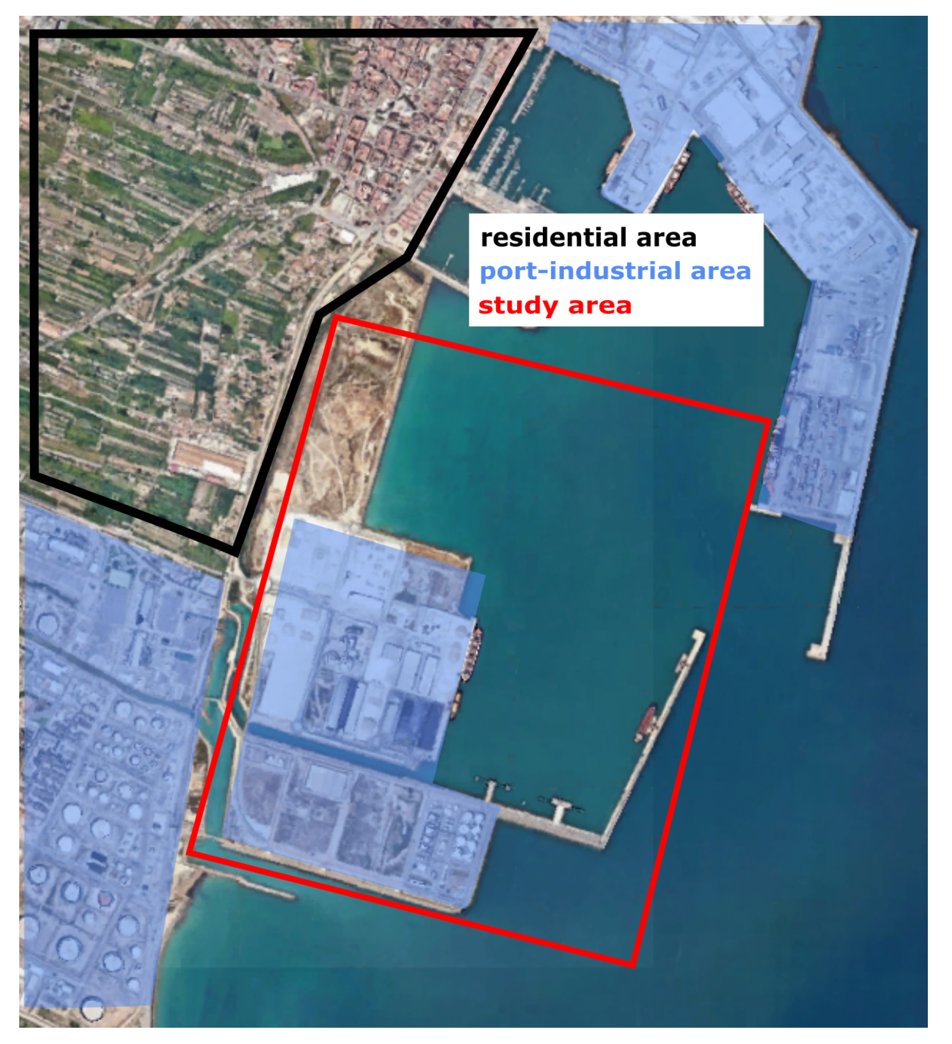
Figure 2.
3D geometric model generation: a) Aerial view of the study area; b) Data point LiDAR; c) Cadastral data; d) Corresponding computational 3D geometry.
Figure 2.
3D geometric model generation: a) Aerial view of the study area; b) Data point LiDAR; c) Cadastral data; d) Corresponding computational 3D geometry.
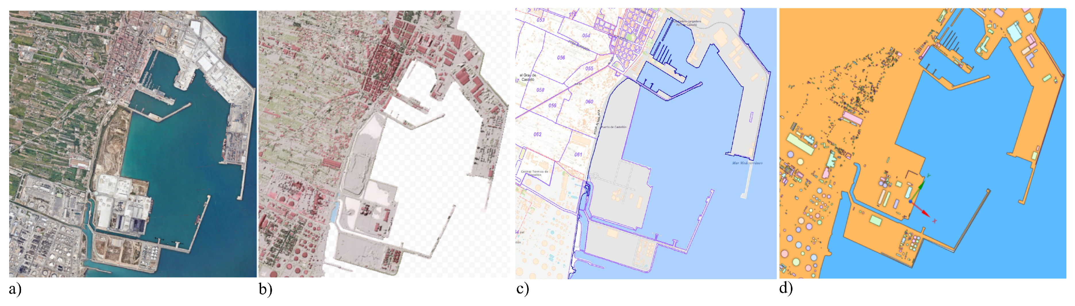
Figure 3.
Computational domain to model the wind flow and particle dispersion.
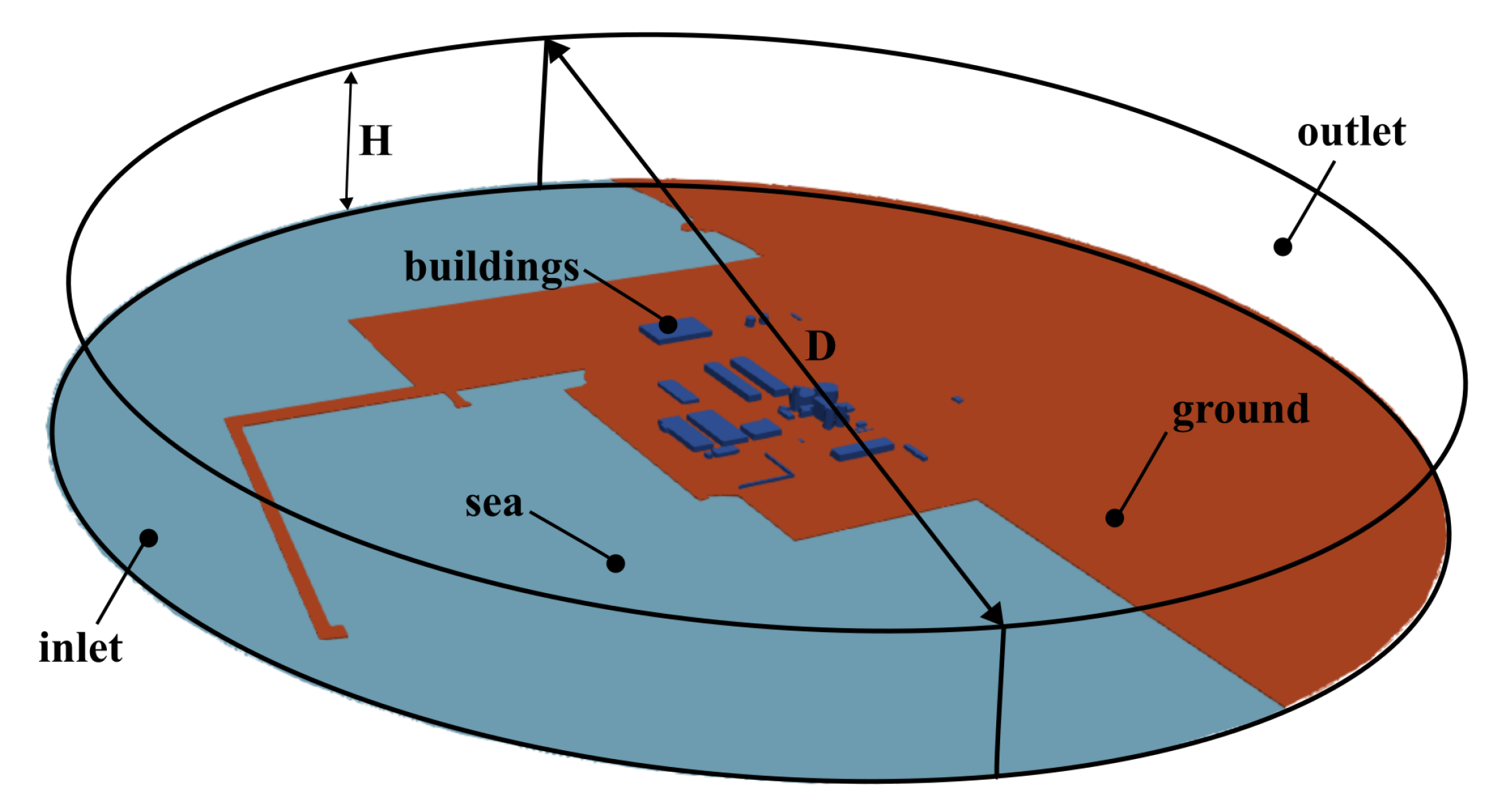
Figure 4.
a) Study area showing wind directions () that affect the adjacent urban area and the locations of two meteorological stations within the computational domain (P1,P2); b) Corresponding wind-direction sector in the wind rose generated from observations collected during 2022–2023 at meteorological station P1.
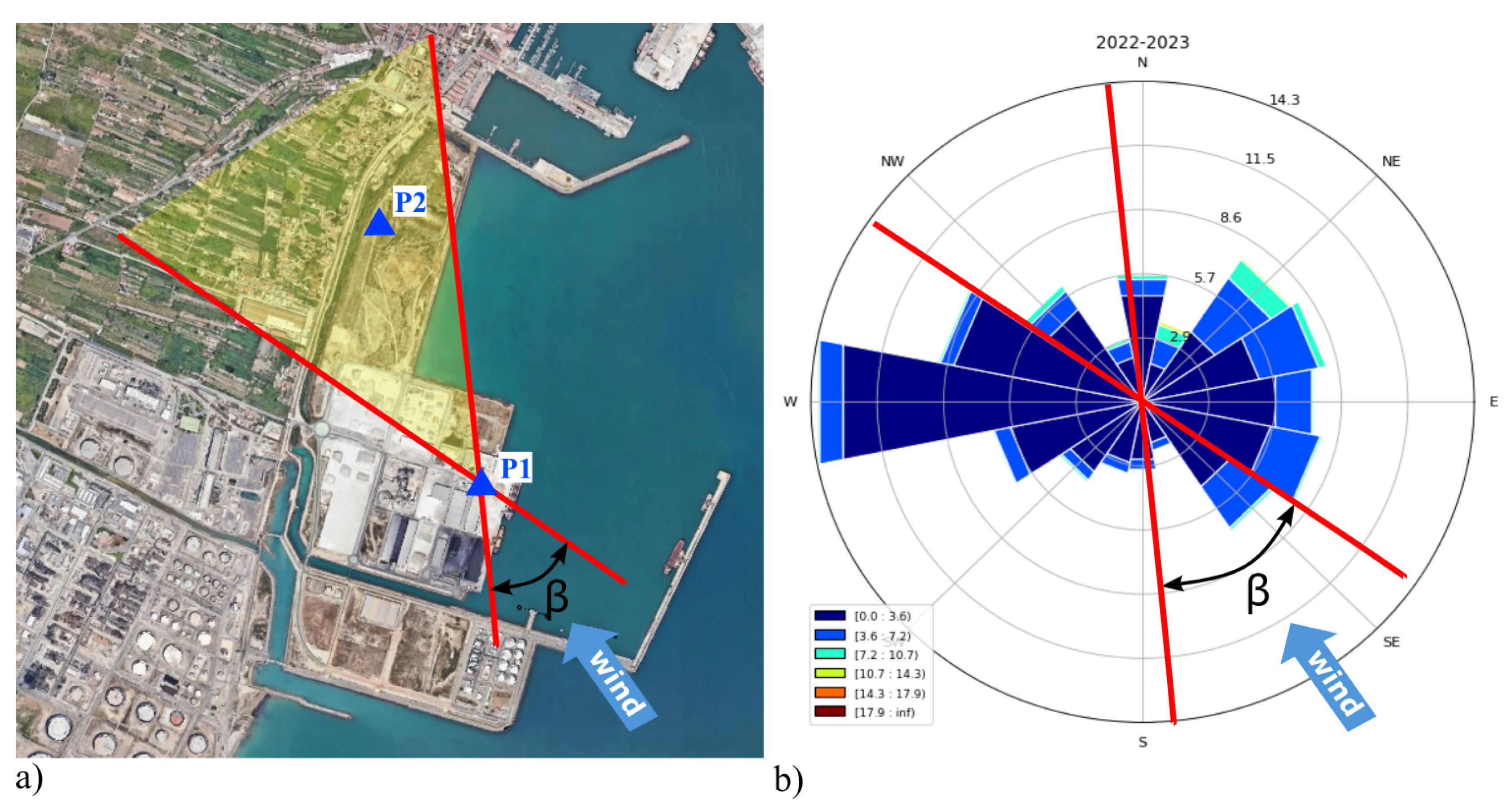
Figure 5.
a) Satellite view of the location of particle sources in study area; b) Location of particle-emission sources (S1-S7) in the computational model; c) Example of truck loading and unloading operations.
Figure 5.
a) Satellite view of the location of particle sources in study area; b) Location of particle-emission sources (S1-S7) in the computational model; c) Example of truck loading and unloading operations.
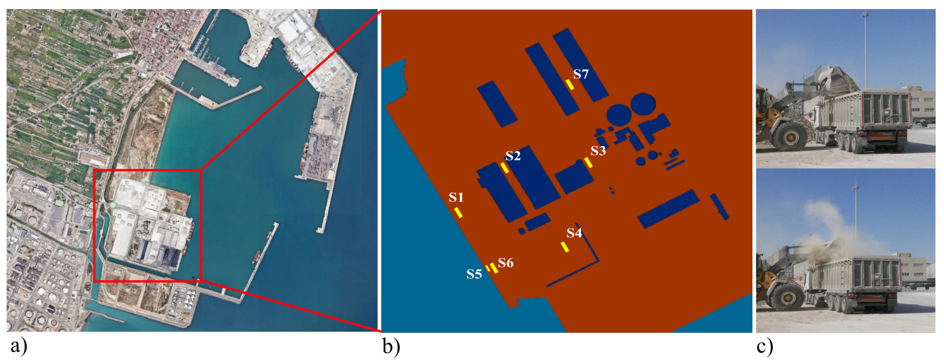
Figure 7.
Hourly wind speed and direction measurements from the reference (P1) and validation (P2) meteorological stations, illustrating the temporal consistency and similarity of atmospheric conditions at both sites.
Figure 7.
Hourly wind speed and direction measurements from the reference (P1) and validation (P2) meteorological stations, illustrating the temporal consistency and similarity of atmospheric conditions at both sites.
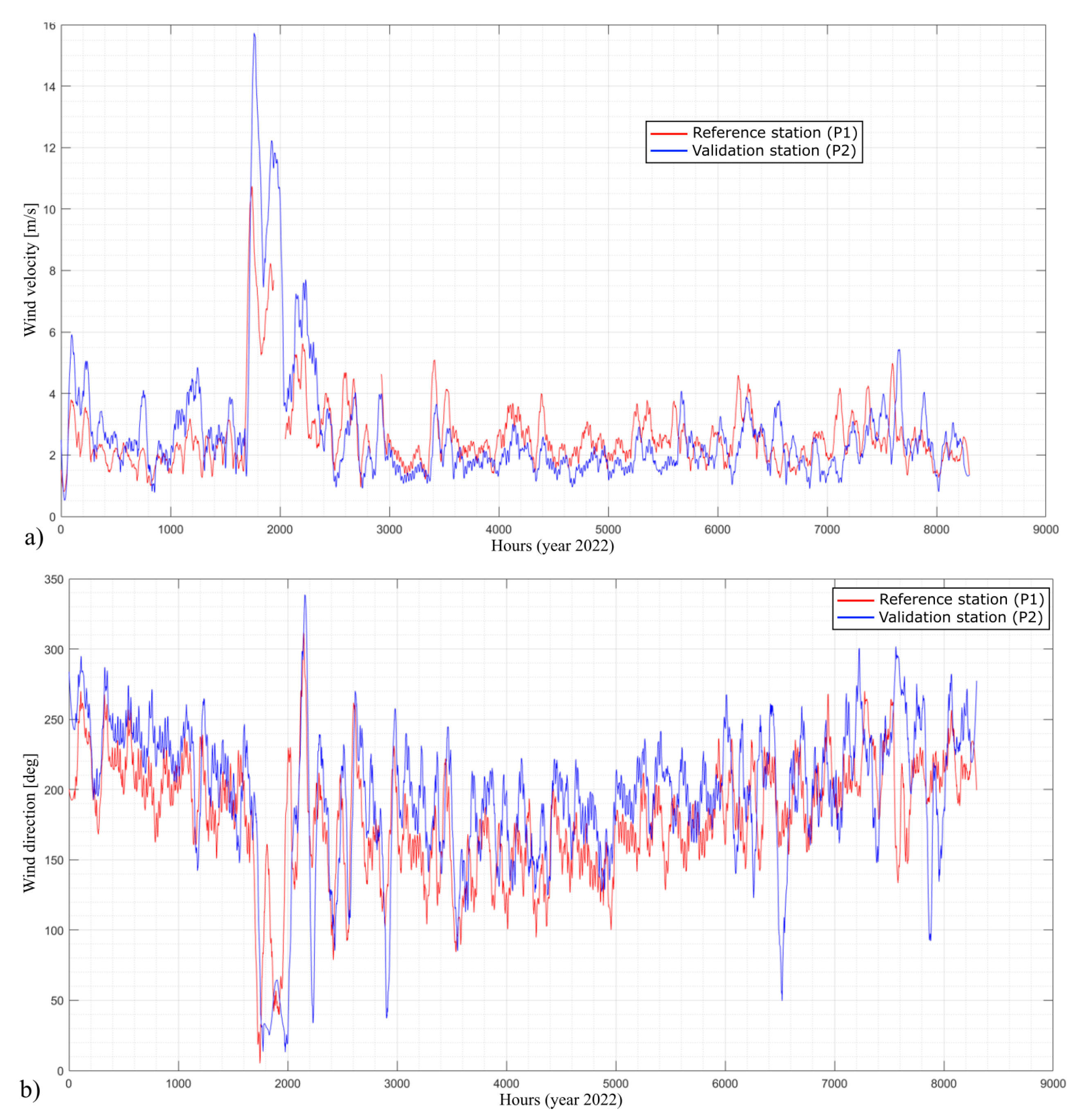
Figure 8.
Histogram of wind speed at the validation station (P2). The red dotted line marks the median value (2.06 m/s), with a standard deviation of = 0.85 m/s
Figure 8.
Histogram of wind speed at the validation station (P2). The red dotted line marks the median value (2.06 m/s), with a standard deviation of = 0.85 m/s
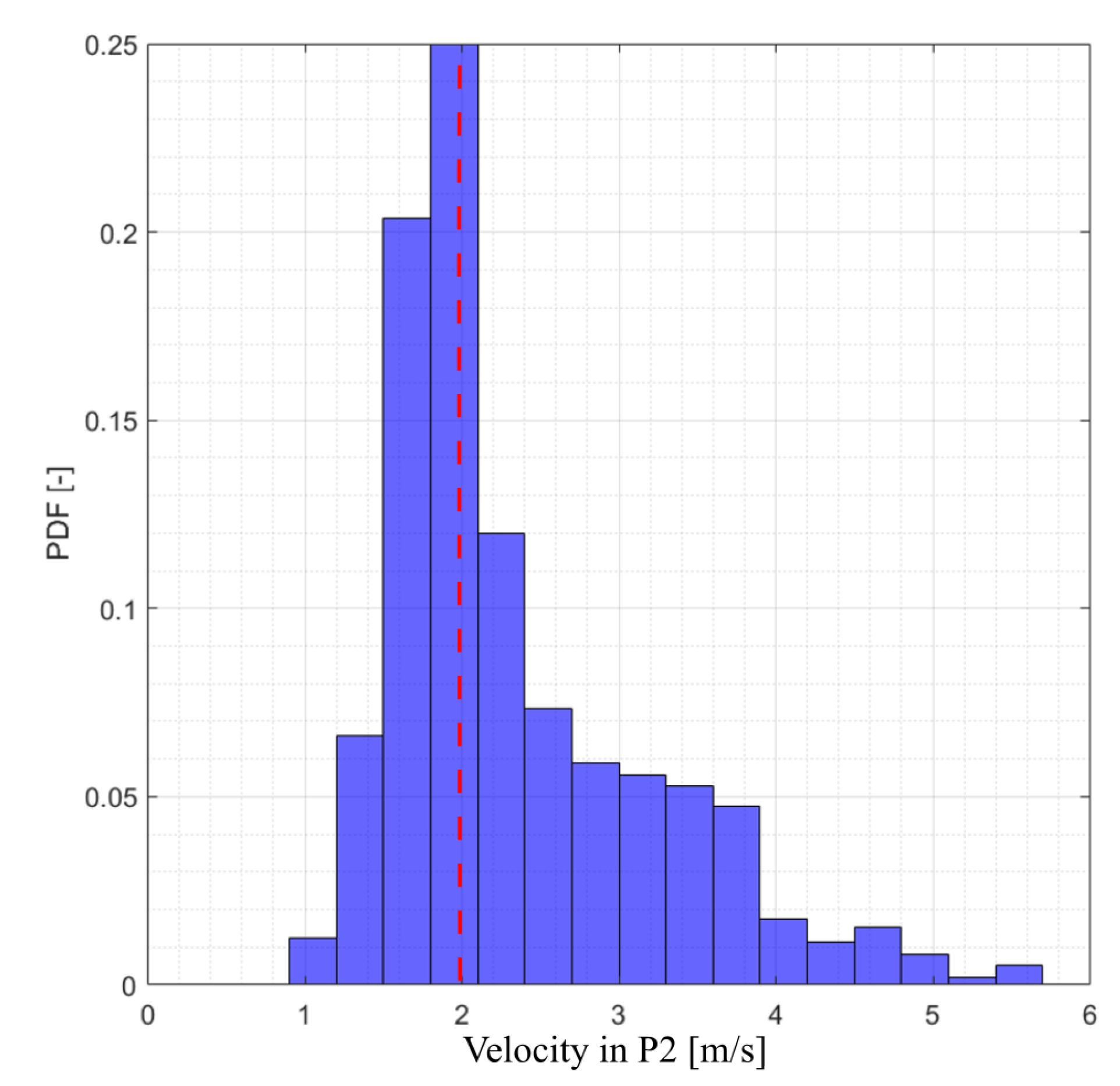
Figure 9.
Methodology followed to process the data from the raw 3D CFD simulations to the 2D fields ready to feed the ML model.
Figure 9.
Methodology followed to process the data from the raw 3D CFD simulations to the 2D fields ready to feed the ML model.
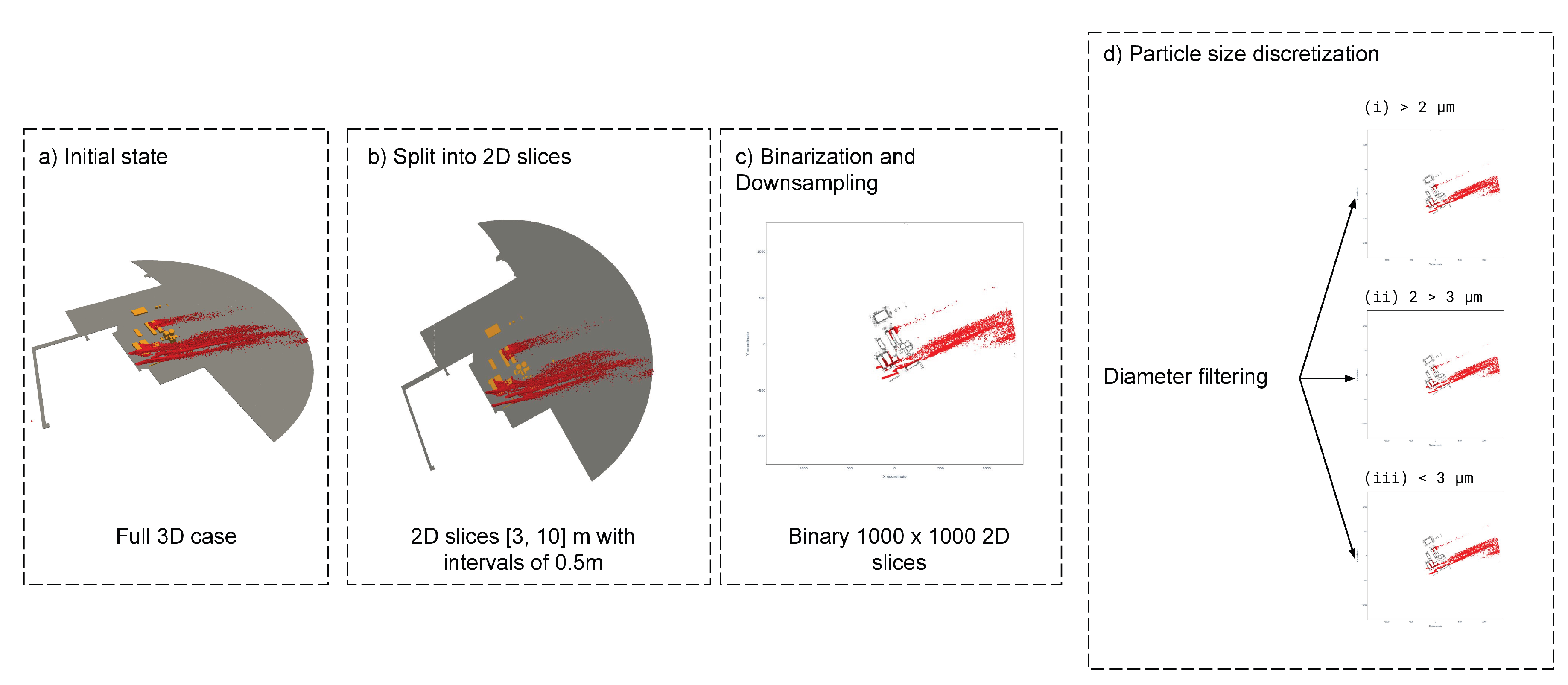
Figure 10.
ML model architecture with the expected input and output together with the dimensionality of each of the ML layers.
Figure 10.
ML model architecture with the expected input and output together with the dimensionality of each of the ML layers.
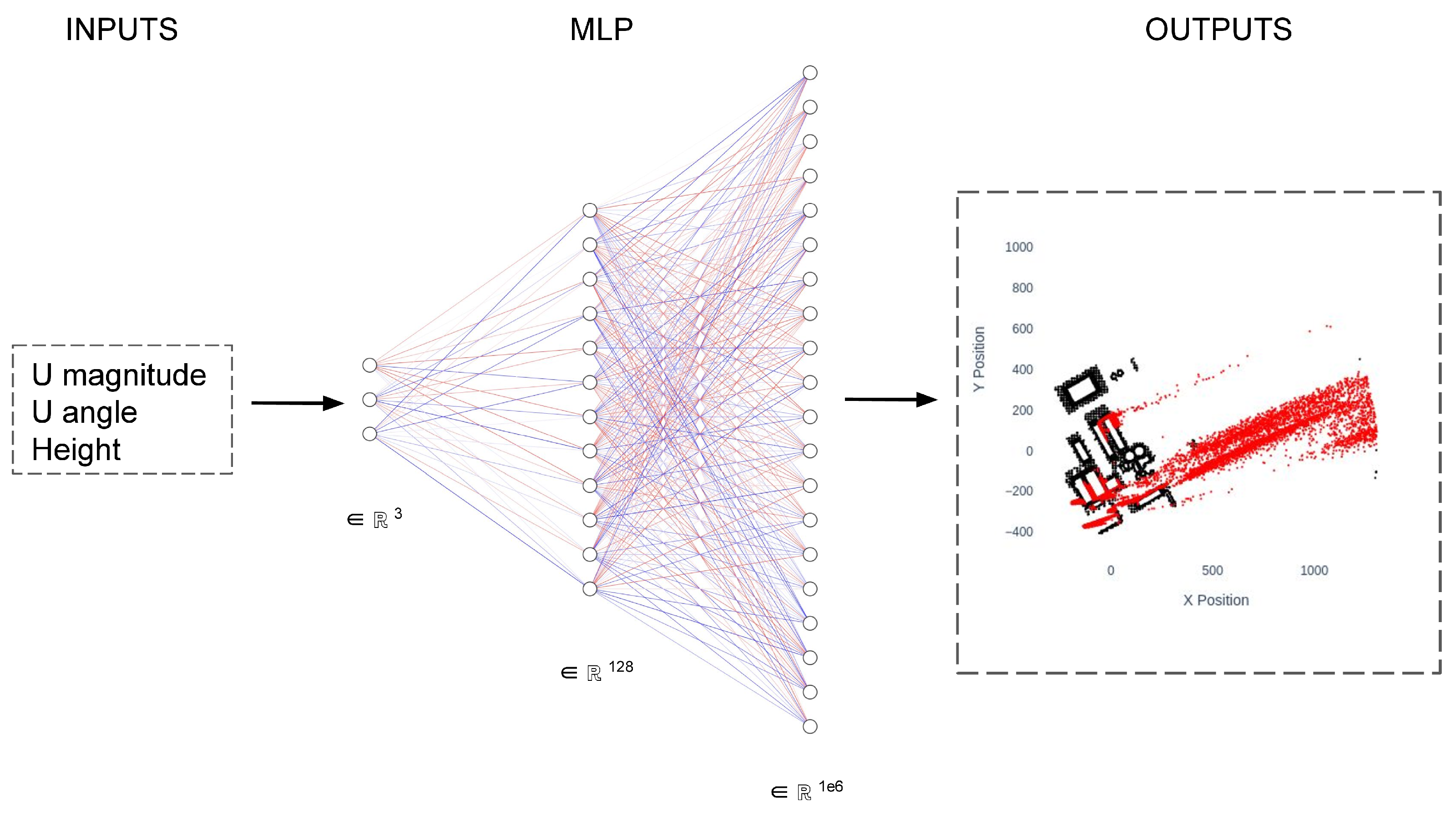
Figure 11.
An example of the converged CFD solution (left) velocity contours and (right) particles, overlayed in a 3D model of the urban environment for the port.
Figure 11.
An example of the converged CFD solution (left) velocity contours and (right) particles, overlayed in a 3D model of the urban environment for the port.
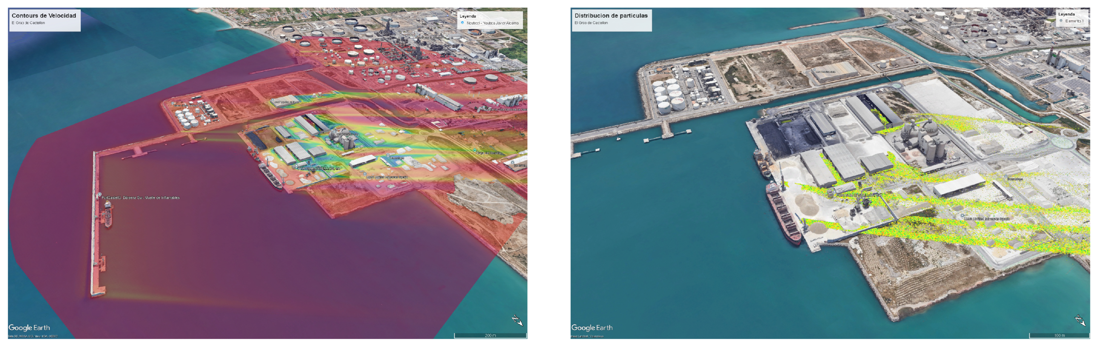
Figure 12.
Graphs illustrating: a) the different particle source placement; b) the particle source diameter distribution, comparing the differences between a velocity of 3 m/s and 6 m/s at point (X=1190m, Y=0m and Z=2m); c) the particle count at each source location for a velocity of 3 m/s; d) a violin plot depicting the downstream evolution (at positions depicted in a) of particle size distribution under varying wind speeds.
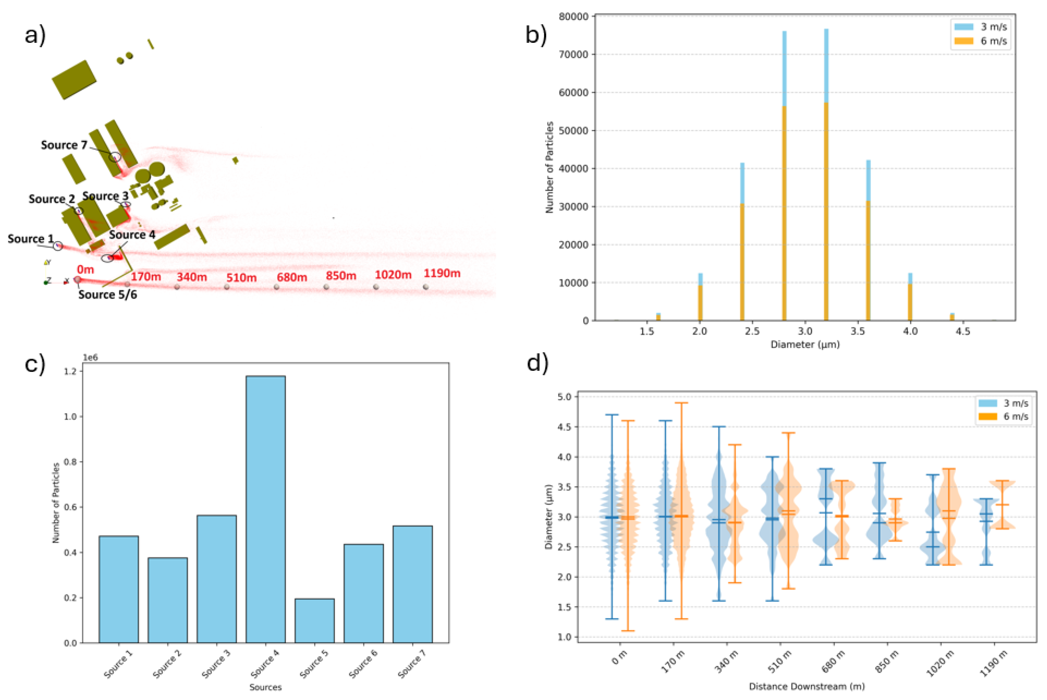
Figure 13.
A velocity vector plot of the entire factory site showing close-ups of (upper-left) Source 4 and (upper-right) Source 3 highlighting a combination of effects created by wind shadowing and circulation.
Figure 13.
A velocity vector plot of the entire factory site showing close-ups of (upper-left) Source 4 and (upper-right) Source 3 highlighting a combination of effects created by wind shadowing and circulation.
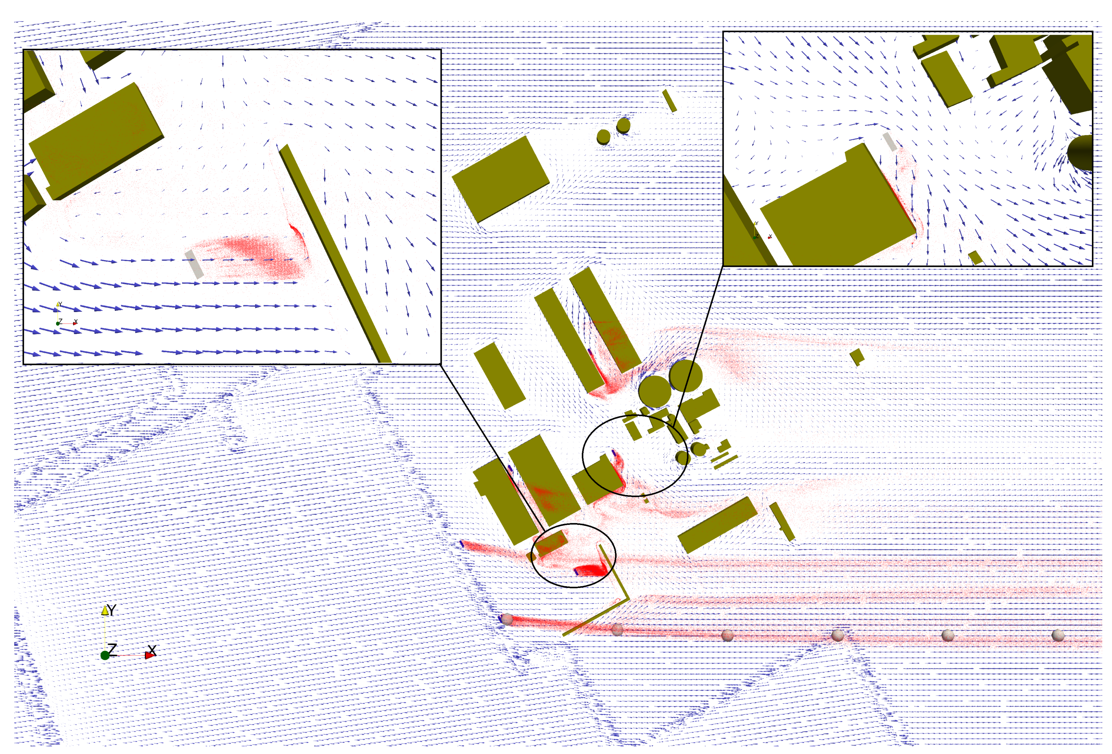
Figure 14.
Comparison of flow dynamics and particle dispersion at varying directions ( = 15°, 0° and -15°) and fixed 3m/s inlet velocity. First row shows the U velocity field magnitude while second row shows the velocity together with the particles field. Also, the buildings are shown in orange.
Figure 14.
Comparison of flow dynamics and particle dispersion at varying directions ( = 15°, 0° and -15°) and fixed 3m/s inlet velocity. First row shows the U velocity field magnitude while second row shows the velocity together with the particles field. Also, the buildings are shown in orange.
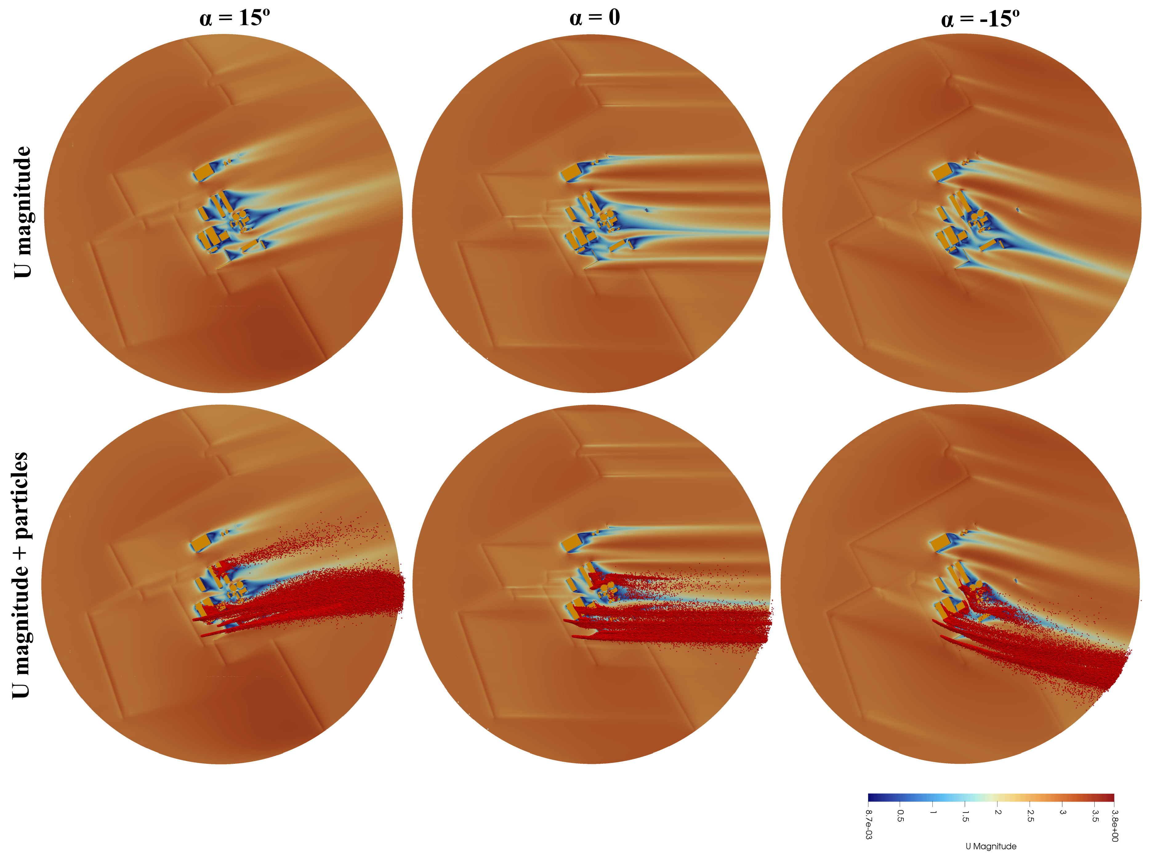
Figure 15.
Ground truth CFD vs. prediction of ML at 6.5m height slice, 6 m/s input velocity, and angles [20, 0, -20] degrees together with the True Positives. The particle diameter represented is between 2 µm and 3 µm.
Figure 15.
Ground truth CFD vs. prediction of ML at 6.5m height slice, 6 m/s input velocity, and angles [20, 0, -20] degrees together with the True Positives. The particle diameter represented is between 2 µm and 3 µm.
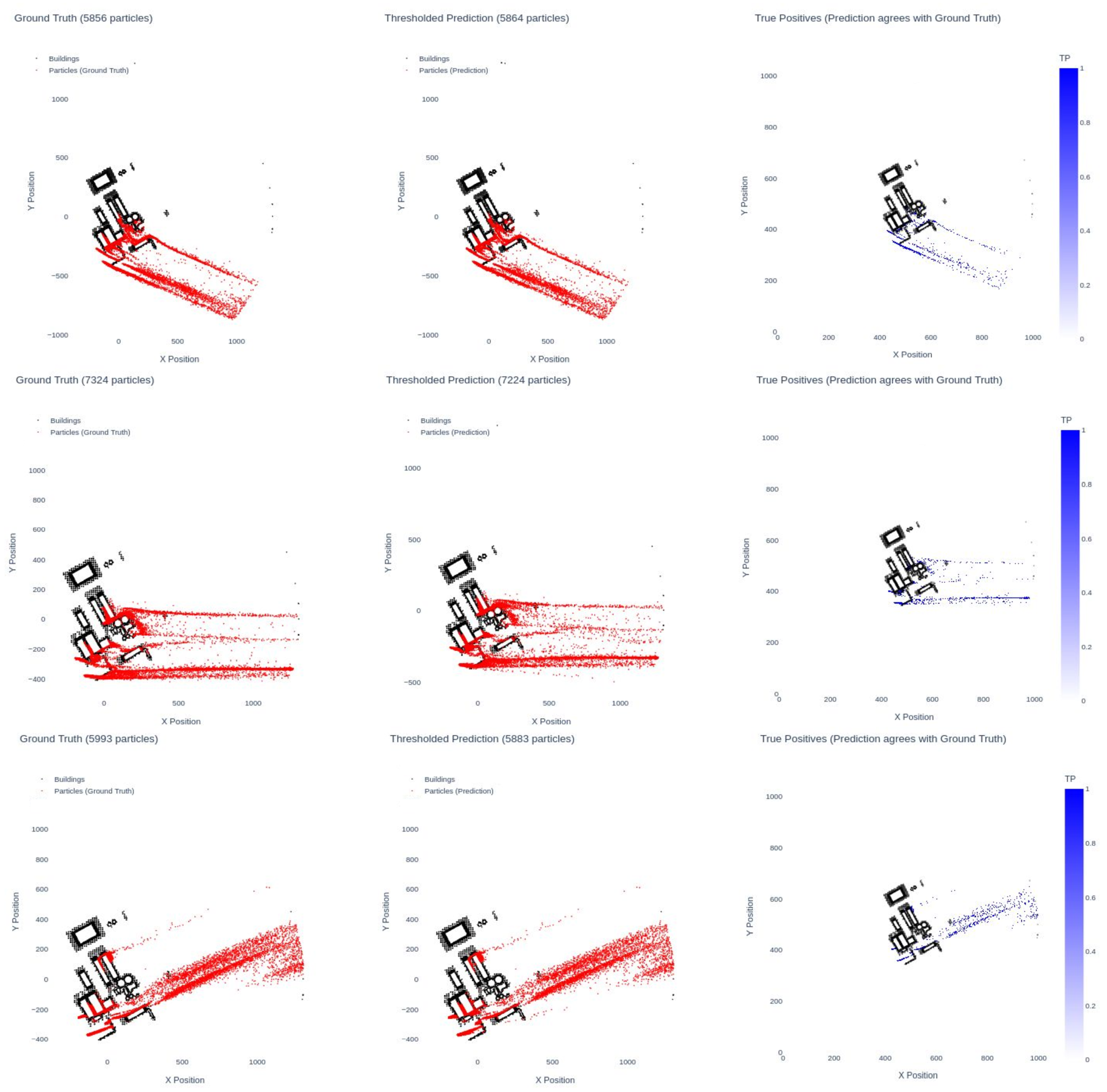
Figure 16.
Confusion matrix for the ML model. The results shown represent the mean across the different validation cases for all three surrogate models.
Figure 16.
Confusion matrix for the ML model. The results shown represent the mean across the different validation cases for all three surrogate models.
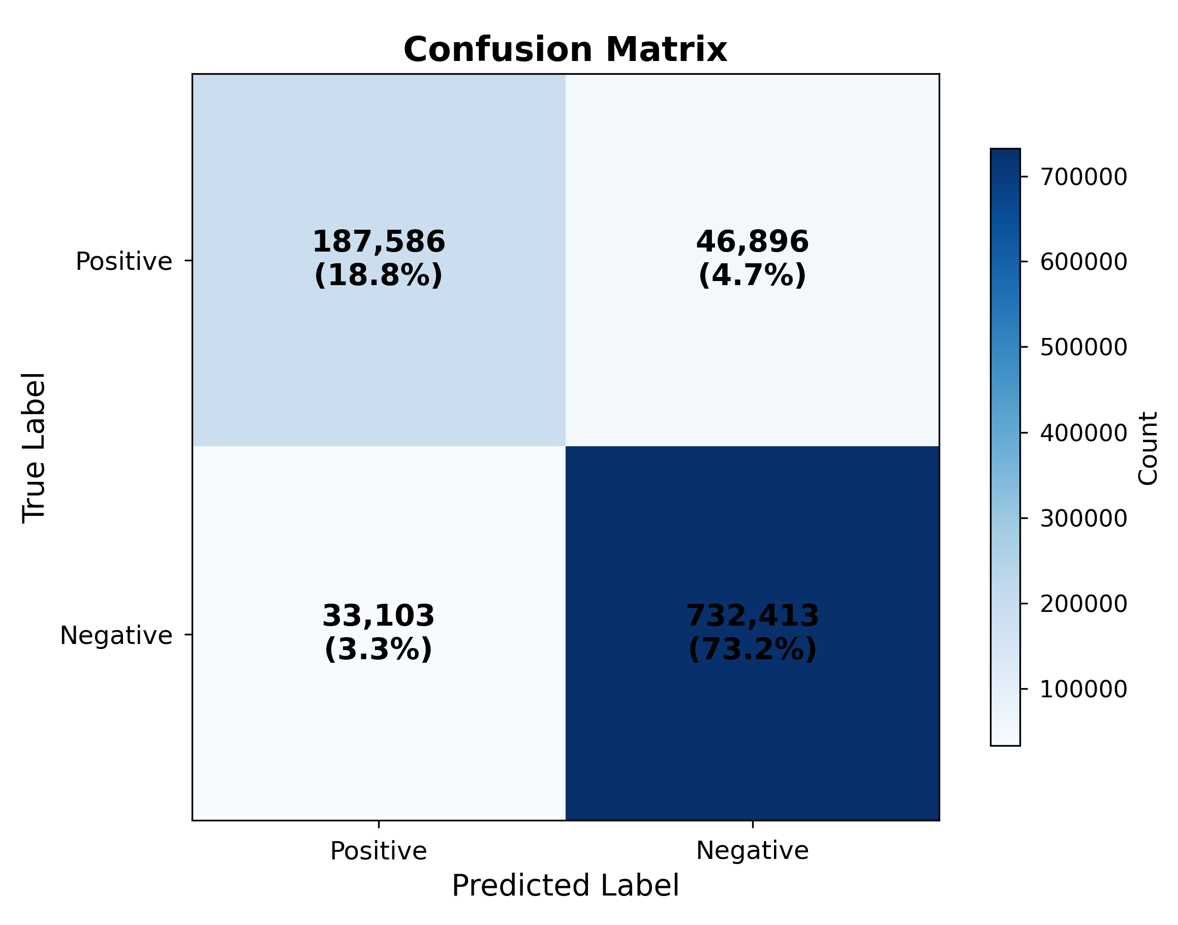
Figure 17.
Spatial distribution of confusion matrix derived metrics for the evaluation case (, wind speed 6.5 m/s, particle diameter 2–3 µm, height slice 6.5 m: a) TNR; b) NPV; c) FPR; d) FNR.
Figure 17.
Spatial distribution of confusion matrix derived metrics for the evaluation case (, wind speed 6.5 m/s, particle diameter 2–3 µm, height slice 6.5 m: a) TNR; b) NPV; c) FPR; d) FNR.
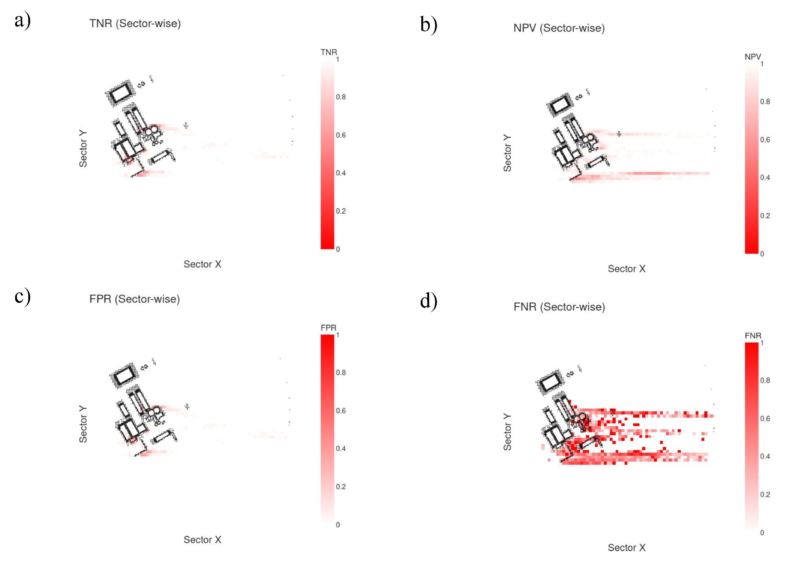

Table 1.
Details of the boundary conditions imposed for the aerodynamic model. Nomenclature: Cc = Calculated, emp = empty, fSS = fixedShearStress, fV = fixedValue, iF = inletFunction, sP = symmetryPlane, wF = wall-Function, zG = zeroGradient.
Table 1.
Details of the boundary conditions imposed for the aerodynamic model. Nomenclature: Cc = Calculated, emp = empty, fSS = fixedShearStress, fV = fixedValue, iF = inletFunction, sP = symmetryPlane, wF = wall-Function, zG = zeroGradient.
| U | p | k | |||
| inlet | iF | zG | iF | iF | Cc |
| outlet | zG | fV | zG | zG | Cc |
| top | fSS | zG | zG | zG | Cc |
| buildings | fV | zG | wF | wF | wF |
| ground and sea | fV | zG | wF | wF | wF |
Table 2.
Lagrangian particle injection parameters used in the dispersion simulations for each source (S1–S7).
Table 2.
Lagrangian particle injection parameters used in the dispersion simulations for each source (S1–S7).
| Property | Value |
|---|---|
| Injection duration (s) | 500 |
| Concentration | 0.6 |
| Parcels per second | 500 |
| Mean particle diameter (m) | |
| Particles per parcel | 500 |
Table 3.
Input and validation data employed in the aerodynamic CFD simulation, including inlet wind conditions and the corresponding wind speed and direction measurements at the reference (P1) and validation (P2) stations.
Table 3.
Input and validation data employed in the aerodynamic CFD simulation, including inlet wind conditions and the corresponding wind speed and direction measurements at the reference (P1) and validation (P2) stations.
| Inlet wind condition | Reference station (P1) | Validation station (P2) | |
| Velocity (m/s) | 2 | ; m/s | ; m/s |
| Direction (°) | 150 | ; m/s | ; m/s |
Table 4.
Quantitative insights from particle size analysis at various locations and wind speeds. The table compares median particle sizes, size ranges, and key observations between 3 m/s and 6 m/s wind conditions.
Table 4.
Quantitative insights from particle size analysis at various locations and wind speeds. The table compares median particle sizes, size ranges, and key observations between 3 m/s and 6 m/s wind conditions.
| Location | Parameter | 3 m/s | 6 m/s |
|---|---|---|---|
| Initial (0 m) | Median Particle Size (m) | ≈ 3.0 | ≈ 3.0 |
| Range of Particle Sizes (m) | 1.5–4.8 | 1.5–4.8 | |
| Insight | Similar particle size distribution at the source for both wind speeds. | ||
|
Early Downstream (170 m) |
Median Particle Size (m) | ≈ 3.0 | ≈ 3.1 |
| Range of Particle Sizes (m) | 1.8–4.5 | 1.6–4.7 | |
| Insight | 6 m/s wind retains slightly larger particles, with a wider range. | ||
|
Midstream (510 m) |
Median Particle Size (m) | ≈ 2.8 | ≈ 2.9 |
| Range of Particle Sizes (m) | 1.5–4.2 | 1.5–4.5 | |
| Insight | Both wind speeds show removal of larger particles, with 6 m/s retaining them longer. | ||
|
Midstream (850 m) |
Median Particle Size (m) | ≈ 2.7 | ≈ 2.8 |
| Range of Particle Sizes (m) | 1.5–3.8 | 1.5–4.0 | |
| Insight | Larger particles are progressively removed. | ||
|
Long-Range Transport (1020–1190 m) |
Median Particle Size (m) | ≈ 2.5 | ≈ 2.6 |
| Range of Particle Sizes (m) | 1.5–3.5 | 1.5–3.7 | |
| Insight | Both wind speeds carry primarily fine particles (≈ 2.5 m). Aerodynamic filtering removes larger particles, stabilizing smaller ones. | ||
Table 5.
Mean classification metrics (F1 score and Precision) for the predictions of all three surrogate models across different wind angles . Values are averaged over all validation cases.
Table 5.
Mean classification metrics (F1 score and Precision) for the predictions of all three surrogate models across different wind angles . Values are averaged over all validation cases.
| F1 | Precision | |
|---|---|---|
| 0.82 | 0.76 | |
| 0.82 | 0.85 | |
| 0.84 | 0.83 | |
| 0.80 | 0.85 | |
| 0.83 | 0.85 |
Table 6.
Metrics computed from the aggregated (mean) confusion matrix: TP=187,586; TN=732,413; FN=46,896; FP=33,103.
Table 6.
Metrics computed from the aggregated (mean) confusion matrix: TP=187,586; TN=732,413; FN=46,896; FP=33,103.
| Metric | Value |
|---|---|
| Accuracy | 0.9200 |
| True Negative Rate (TNR) | 0.9568 |
| Negative Predictive Value (NPV) | 0.9398 |
| False Positive Rate (FPR) | 0.0432 |
| False Negative Rate (FNR) | 0.2 |
Disclaimer/Publisher’s Note: The statements, opinions and data contained in all publications are solely those of the individual author(s) and contributor(s) and not of MDPI and/or the editor(s). MDPI and/or the editor(s) disclaim responsibility for any injury to people or property resulting from any ideas, methods, instructions or products referred to in the content. |
© 2025 by the authors. Licensee MDPI, Basel, Switzerland. This article is an open access article distributed under the terms and conditions of the Creative Commons Attribution (CC BY) license (https://creativecommons.org/licenses/by/4.0/).
Copyright: This open access article is published under a Creative Commons CC BY 4.0 license, which permit the free download, distribution, and reuse, provided that the author and preprint are cited in any reuse.


