Submitted:
19 November 2025
Posted:
20 November 2025
You are already at the latest version
Abstract
The investigation of lunar polar regions is critical for understanding the characteristics of the moon, such as the crustal evolution, volatile retention, and in-situ resource utilization. In addition, it serves as an important reference and prerequisite for future lunar exploration missions and the establishment of a long-term scientific research station. However, quantitative multi-oxide mapping in these regions remains limited since previous efforts mainly focused on FeO at coarse spatial resolutions (~1 km/pixel). To address this gap, an inversion model for a one-dimensional convolutional neural network (1D-CNN) to obtain high-resolution (~500 m/pixel) abundance distributions of six major oxides—FeO, TiO₂, Al₂O₃, CaO, MgO, and SiO₂—across the lunar polar regions (65°–90°N/S) is investigated in this research. The developed 1D-CNN model, utilizing the KAGUYA SP hyperspectral data and oxide results from Bian et al. (2025) as sample data, achieved high inversion accuracy, as evidenced by R² > 0.94 for all oxides and RMSE < 0.3 wt.% except for Al₂O₃. The inverted oxide maps reveal that the materials in the south polar region (83°–90°S) are compositionally uniform and dominated by feldspathic highland lithologies, which are distinct from the ejecta or mantle-derived materials typically associated with the South Pole–Aitken basin. These results provide a new insight into the crustal origin of the lunar south pole. Moreover, comparisons of the nine Artemis Ⅲ candidate landing regions showed overall compositional homogeneity, suggesting similar highland-derived sources, and of the nine regions, the Slater Plain and de Gerlache Rim 2 areas were identified as optimal targets for capturing resource diversity within feasible operational ranges. These findings not only fill a critical gap in quantitative geochemical mapping of the lunar poles but also provide essential references for the Artemis Ⅲ and Chang’E-7 missions, supporting landing region selection for future missions, resource evaluation, and in-situ utilization strategies.
Keywords:
Lunar polar regions
; Oxide abundance inversion
; 1D-CNN deep learning
; KAGUYA SP hyperspectral data
; Artemis III landing regions
1. Introduction
The chemical composition of the lunar polar regions holds critical implications for understanding the Moon’s geological evolution, volatile distribution, and in-situ resource potential (Zhang et al., 2023). In recent years, the lunar south pole, especially in the region above 85°S latitude, has become a primary target for lunar exploration due to its unique illumination environment, potential volatile reservoirs, and preserved ancient crustal materials (Wang et al., 2024). In particular, the lunar south pole has become a major focus of current and future exploration missions including NASA’s Artemis Ⅲ and China’s Chang’E-7 (CE-7) missions, both of which are scheduled for launch around 2026 (NASA, 2024; Wang et al., 2024). The Artemis Ⅲ mission aims to achieve a crewed landing within the 83°–90°S region, while the CE-7 mission is designed to conduct environmental and resource surveys in the lunar south polar region of the Aitken Basin at latitudes above 85°S.
Currently, since high-resolution quantitative mapping for multi-oxide abundances in the lunar south pole regions remains underdeveloped, the understanding of crustal composition and resource distribution in these regions is limited. Early efforts, e.g., Lawrence et al. (2002) used LP-GRS and neutron spectrometer data to derive FeO abundance maps of the lunar poles, but their results were constrained by a coarse spatial resolution (~15 km/pixel) and uncertainties in calibration under extreme illumination conditions. With the polar regions emerging as strategic priorities for future surface operations and base construction, there is a pressing need for fine-scale, multi-oxide compositional mapping to support landing site selection and mission planning (Zeeshan et al., 2021).
Although high-spatial-resolution optical data have been acquired by multiple lunar orbiters, the harsh illumination environment, characterized by permanently shadowed regions, and also the low signal-to-noise ratios pose severe challenges for conventional reflectance-based inversion techniques (Lucey et al., 2021). Currently, it is unlikely to find such a single instrument that provides high spatial resolution and also radiometric stability in the polar environment.
To overcome the above mentioned problem, Lemelin et al. (2022) developed an innovative approach combining KAGUYA’s Spectral Profiler (SP) data with Lunar Orbiter Laser Altimeter (LOLA) reflectance measurements to produce a 1 km/pixel FeO abundance map, which led to an improved radiometric accuracy. Validation against LP-GRS data demonstrated that the approach yields consistent results, which establishes a foundation for subsequent investigations. However, all past research mainly focused on FeO, while other major oxides, e.g., TiO₂, Al₂O₃, MgO, CaO, and SiO₂, have not yet been inverted at a comparable resolution or accuracy.
Furthermore, machine learning and deep learning techniques, which have become increasingly important tools in planetary remote sensing, require large, diverse, and representative training datasets (Bickel et al., 2021). However, such datasets remain scarce for the lunar polar regions due to the absence of in-situ measurements and returned samples (Zhang et al., 2025). As emphasized by Qiu et al. (2022), the construction of representative oxide sample datasets can greatly advance lunar surface composition inversion, and future progress will rely on multi-mission data integration, augmentation, and fusion.
In this context, this study applied a 1D-CNN deep learning framework to hyperspectral data from KAGUYA SP and the reference data of six major oxides—FeO, TiO₂, Al₂O₃, MgO, CaO, and SiO₂ from mid-latitude regions reported by Bian et al. (2025) to construct a sample dataset for the polar regions. Its resultant high-resolution (~500 m/pixel) inversion model established for each of the six oxides was then used to generate distribution maps for the 65°–90°N/S regions. To the best of our knowledge, this work provides the first comprehensive set of abundance maps for six major oxides across the lunar polar regions, offering new insights into the composition and evolution of the polar crust, as well as valuable references for future landing site selection and in-situ resource utilization planning.
2. Materials and Methods
2.1. KAGUYA SP Hyperspectral Data
The SP onboard the KAGUYA lunar explorer collects reflectance spectra from the lunar surface in the visible to near-infrared spectral range (500–2600 nm), with a spatial resolution of approximately 500 m/pixel (Haruyama et al., 2008). The instrument utilizes two gratings and three linear array detectors: one visible detector (VIS, 500–1000 nm) and two near-infrared detectors (NIR1, 900–1700 nm; NIR2, 1700–2600 nm) (Yamamoto et al., 2014). Between 2007 and 2009, the sensor conducted continuous spectral observations across the visible to near-infrared wavelengths of the Moon. However, due to the complex illumination conditions in the lunar polar regions, both the coverage and quality of SP data are somewhat limited in these areas. For example, while the radiometric calibration performed by Yamamoto et al. (2011) on the VIS and NIR1 spectral ranges of the SP data yielded high-quality results, the same background removal method introduced significant noise in the NIR2 spectral range Yamamoto et al. (2011). Therefore, in this study, the 150-band VIS and NIR1 spectral data processed by Lemelin et al. (2022), which builds upon the method of Yamamoto et al. (2011) with additional high-noise removal and spectral smoothing, were used as the data foundation for estimating oxides in the lunar polar regions. These spectral data have been demonstrated to yield reliable estimates of lunar minerals and oxides (Lemelin et al., 2022).
2.2. Sample Selection and Pre-Processing
Currently, no lunar soil samples from the 65°–90° latitude regions have been returned to the earth by human missions. Furthermore, due to the challenging observational conditions at the lunar poles, such as limited illumination and the restricted coverage of available spectral image data, studies on the inversion of oxide abundances in these polar regions remain scarce. This section aims to construct paired datasets consisting of hyperspectral images (as inputs) and corresponding oxide abundances (as outputs) to establish an inversion model for six major oxides—FeO, TiO₂, Al₂O₃, CaO, MgO, and SiO₂—within the 65°–90° latitude range.
Figure 1 shows the initial oxide abundances (a) and hyperspectral images (b) from which the above mentioned sample dataset was selected. Subfigure (a) presents the FeO distribution from the high-resolution oxide abundance maps covering the latitude range from 65°N–65°S produced by Bian et al. (2025), while (b) is the SP data processed by Lemelin et al. (2022) spanning latitudinal zones 50°–90°N and 50°–90°S. The overlapping region between the two datasets is the 50°–65°N/S latitudinal band (see the blue shaded areas in both subfigures); pixels within this region were therefore selected as the sample data to establish the inversion model proposed by this study. It should be noted that the upper and lower boundaries shown in subfigure (a) correspond to 65°N and 65°S, respectively.
The rules for constructing the polar oxide abundance dataset in this study are summarized as follows. To mitigate potential data uncertainties near image boundaries, the sampling region was defined between 170°W and 170°E in longitude with a 5° interval (yielding 69 longitudinal lines), and between 51° and 64°N/S in latitude with a 1° interval (yielding 28 latitudinal lines). The intersections of these longitudinal and latitudinal lines served as the sample points.
To enhance the representativeness of spectral reflectance data from the SP dataset, the mean reflectance of the nearest 2×2 pixels surrounding each sample point was extracted from the SP images to reduce random errors. To ensure spatial consistency in the sample extraction, the same procedure was also applied to the oxide abundance maps – the mean value within a 17×17-pixel neighborhood around the sample point was taken as the oxide abundance for the sample point. This process further facilitates the extraction of sample data from the sample region.
To ensure the quality of the sample dataset, the above sample points were further screened by comparing their FeO abundance values with those derived from the FeO abundance maps inverted by Lemelin et al. (2022). Specifically, only those data whose ratio of the absolute difference between the two FeO values to the smaller of the two was less than 0.1 were retained. This process resulted in 940 sample points remaining in the dataset, which served as the final samples used to establish the inversion model.
2.3. Correlation Analysis
To assess the validity of input image features for the oxide abundance inversion, the Pearson correlation coefficient (R) was used to evaluate the correlation between the reflectance values from the SP image and oxide abundances contained in the sample dataset obtained from Section 2.2. Since this coefficient is a mean-centered result, it can reduce the impact of scale differences between two variables on similarity measurement (Bian et al., 2022). The equation for R is:
where is the number of samples; is the index of oxide sample; and are the oxide abundance and reflectance values of the th sample, respectively; and are the mean of all and , respectively. The absolute value of , ||, indicates the strength of correlation between the two variables. The closer the || value to 1, the stronger the correlation between the two variables (Fieller et al., 1957).
According to Bian et al. (2024), the varying degrees of correlation between reflectance at different spectral bands and oxide abundances can, to some extent, influence the accuracy of oxide inversion on the lunar surface. In this study the correlation coefficients between the 150 spectral bands and six oxide abundances for the 940 sample points were calculated using Eq. (1) and the results are shown in Figure 2. We can see that, except for SiO₂, which shows a low correlation coefficient value, the other five oxides had large values, especially Al₂O₃ and FeO. In addition, the coefficient values in bands 41–150 are larger than those in bands 1–40.
2.4. D-CNN Algorithm
A convolutional neural network (CNN) is a type of feedforward neural network characterized by convolutional computations and deep architecture. As one of the representative algorithms in deep learning, it is widely applied in computer vision, image processing, and other fields. Thanks to its unique structure, CNN can automatically learn spatial hierarchical features from input data, enabling outstanding performance in classification or regression tasks such as image classification, object detection, and parameter inversion. CNNs are generally implemented in one-dimensional (1D), two-dimensional (2D), or three-dimensional (3D) forms, depending on the nature and dimensions of input data.
The selection among 1D, 2D, or 3D CNN architectures is dictated not merely by the inherent dimensions of the data, but more fundamentally by the specific task objectives and the nature of the relationships to be modeled. While 2D or 3D CNNs are typically suited for data with dependencies across adjacent spatial positions, the inversion of lunar oxides requires consideration of the specific application context. The core objective of this study—inverting oxide abundances on the lunar polar surface—involves establishing relationships between multi-band reflectance (spectral dimension) at sample points and oxide abundances. This task aligns more closely with the application scope of 1D-CNN, as it depends less on adjacent spatial relationships (Zhang et al., 2023). In this framework, the 150-band reflectance values of each SP image pixel were treated as a one-dimensional sequence, with the primary goal being to invert oxide abundances from these 1D spectral sequences. Moreover, using 1D-CNN helps avoid extracting irrelevant information from images, thereby improving the learning efficiency of the neural network (Yang et al., 2023). Therefore, this study employed a 1D-CNN to construct a nonlinear regression model for the relationship between the band-wise reflectance of selected SP image samples and different oxide abundances.
The 1D-CNN architecture used in this study mainly consists of a feature extraction module with five 1D convolutional blocks and a prediction module with a fully connected layer, as illustrated in Figure 3. Each convolutional block includes a 1D convolutional layer, a Batch Normalization (BN) layer, and a ReLU activation function. The number of channels in the convolutional blocks was preset as [n, n, 2n, 2n, 4n] to progressively extract higher-level features. Based on empirical knowledge, candidate values for n were set to 16, 32, and 64, representing models of varying sizes. The final value of n was determined based on subsequent model performance. The kernel size was set to 3, the stride to 1, and zero-padding was applied to ensure the output feature map size matches the input. Following the feature extraction module, a fully connected layer produced the final predictions for the six major oxide abundances.
To ensure effective training of the 1D-CNN model, relevant parameters were configured as follows. During training, the Adam optimizer was used to adaptively adjust model weights. The batch size was set to the total number of training samples, and the training was conducted over 100 epochs with a weight decay of 0.0001. In addition, to achieve more reasonable and accurate model training and evaluation, Leave-One-Out Cross-Validation (LOOCV) for model training and accuracy assessment was adopted. Specifically, for a dataset containing N samples (e.g., 940 samples in this study), LOOCV performs N iterations, and in each iteration only one sample was used for validation while the remaining (N–1) samples (e.g., 939 samples in this study) were used for training. Although LOOCV is computationally intensive, it maximizes the use of the dataset for training and provides an unbiased estimate of model performance. Furthermore, inspired by Wortsman et al. (2022), in this study the following model weight averaging strategy was adopted: averaging the weights of all the N models obtained from LOOCV to produce a final model for lunar polar oxide abundance inversion. This strategy helps enhance the generalization capability of the final regression model across different regions (Yang et al., 2023).
2.5. Performance Evaluation
The regression model established in this study was evaluated using the coefficient of determination (R²), root mean squared error (RMSE), and mean absolute error (MAE). R², which ranges from 0 to 1, is commonly utilized to quantify the predictive accuracy of the model, with values closer to 1 indicating better model performance. RMSE measures the deviation between predicted and observed values, which is commonly used to indicate the accuracy of the model. MAE indicates the average magnitude of the deviation. Their formulae are:
where represents the number of samples, denotes the sample index, and are the measured and inverted oxide abundances of the th sample, respectively, and and are the means of all and values, respectively.
3. Results
3.1. Optimal Configuration of Hyperparameters for 1D-CNN Model
To determine the optimal values for hyperparameters used in the 1D-CNN model, experiments based on various numbers of convolutional channels and learning rates were conducted for comparisons. Table 1 presents the model performance for channel configurations [n, n, 2n, 2n, 4n] (n = 16, 32, 64), with the learning rate fixed at 0.001. The results indicate that n = 32 yields the highest R² and lowest RMSE values for all six oxides, suggesting that this configuration is optimal. Moreover, it offers higher computational efficiency compared to n = 64.
Similarly, Table 2 shows the results from the cases of varying learning rates [0.01, 0.001, 0.0001] but a fixed number of channels (n=32). One can find that the optimal performance is from the learning rate of 0.001. Note that larger learning rates may lead to unstable convergence, while smaller values may lead to slower training and weaker generalization.
Figure 4 shows the scatter plots of predicted values (from the optimal configuration: learning rate = 0.001, n = 32) versus observed values for all 940 sample points, exhibiting excellent consistency along the 1:1 line. Table 3 summarizes the corresponding statistical results, showing that all Rs exceed 0.97 and MAEs are below 0.16 wt.%. Although the RMSE of Al₂O₃ (0.402 wt.%) is slightly higher, the overall inversion accuracy is desirable for lunar oxide mapping in the polar regions.
3.2. Results of FeO
Based on the above constructed 1D-CNN model for FeO abundance inversion, 150-band SP images covering the 65°–90°N/S latitude ranges were input into the model to generate FeO abundance distribution maps for the regions of (a) the north pole and (b) the south pole, as shown in Figure 5. Note that the lunar polar stereographic projection was adopted in these two distribution maps (and also subsequent maps shown in this study). This projection is centered on either the lunar north or south pole, projecting the lunar surface onto a plane tangent at the projection center. As shown in Figure 5(a), the FeO abundance in the north polar region is generally low, with most areas below 7 wt.%. In contrast, Figure 5(b) shows a clearly different distribution, where the FeO abundance within the 120°W–180°–160°E range is significantly higher than in other areas.
To verify the FeO abundance results shown in Figure 5, Figure 6 shows results obtained from Lemelin et al. (2022) for comparison, and the difference between the two results is shown in Figure 7. It can be seen that in many areas of both poles, the results in Figure 5 are slightly less than that in Figure 6, with less than 1 wt.% absolute difference values in most regions.
Moreover, relatively larger discrepancies are in the SPA basin (mostly within 2 wt.%), whilst our results are closer to the FeO abundances in this region reported by Lawrence et al. (2002) than to those of Lemelin et al. (2022). These differences are most plausibly attributed to methodological and reference dataset variations. Specifically, the nonlinear 1D-CNN inversion model trained on locally derived sample sets can enhance sensitivity to subtle spectral and compositional variations, which may lead to small systematic offsets. In addition, the oxide sample dataset, derived from the inversion results of Bian et al. (2025), may carry inherent uncertainties, which may contribute to the above differences. Nevertheless, the overall spatial patterns and compositional trends of our inversion results show strong agreement with those reported by Lemelin et al. (2022) and Lawrence et al. (2002), indicating that the 1D-CNN inversion model developed in this work is trustworthy and provides a valuable reference for future lunar polar compositional analyses.
3.3. Results of Other Five Oxides
Similar to Section 3.2, in this section, 150-band SP reflectance data were input into the Al₂O₃ inversion model developed based on the 1D-CNN algorithm, and the Al₂O₃ abundance distribution resulting from the model is shown in Figure 8. Unlike the FeO abundance distributions shown in Figure 5, Figure 8 exhibits high abundances covering nearly the entire north polar region and most of the south polar region, indicating a high concentration of plagioclase minerals in these areas. However, lower Al₂O₃ abundances are observed in the north polar region (65°–75°N, 10°–40°E), as well as in the south polar region around the South Pole–Aitken (SPA) basin, the Schrödinger crater (133°E, 74.5°S), and the area between 65°–75°S and 80°–110°E. It is worth noting that the low Al₂O₃ abundance within the SPA basin generally agreed well with the observations of (Sun and Lucey, 2024), who reported that the plagioclase content inside the SPA basin is significantly lower than in its surroundings.
Figure 9 shows the abundance distributions of TiO₂, CaO, MgO, and SiO₂ inverted by the 1D-CNN model (where N and S represent the north and south poles, respectively). Figure 9(a) indicates that the TiO₂ abundance in the lunar north polar region is generally low and spatially uniform. In the south polar region, the distribution of TiO₂ resembles that of FeO shown in Figure 5(b), with significant enrichment within the SPA basin. However, the high-Ti regions are more extensive, with elevated titanium content even across the 80°–90°S range.
Figure 9(b) clearly shows that both the north and south polar regions generally exhibit high CaO abundances. However, the CaO abundance along the inner edge of the SPA basin is significantly lower than that outside it, indicating a higher proportion of low-calcium pyroxene (LCP) inside the rim and a greater abundance of plagioclase on the exterior. This LCP enrichment is interpreted as being potentially associated with ejecta deposits from the SPA impact event. Meanwhile, the Schrödinger crater in the south polar region also exhibits relatively low CaO abundance (~12 wt.%), which agrees well with the finding by (Sun and Lucey, 2024) of abundant orthopyroxene in this area.
Figure 9(c) for the MgO abundance distribution shows that high-MgO areas are in both polar regions, with the SPA basin exhibiting the most pronounced magnesium enrichment (~10 wt.%), indicating a substantial proportion of mafic components, such as olivine or LCP minerals. Figure 9(d) shows that SiO₂ abundances exceed 45 wt.% across nearly all areas of both polar regions. Only in the vicinities of Schrödinger crater, Antoniadi crater (173.06°W, 69.23°S), Dawson crater (135.07°W, 67.04°S), and de Forest crater (162.68°W, 77.07°S) do SiO₂ abundances approach ~44 wt.%.
3.4. Results of Test Using Out-of-Sample Data
To further validate our inversion models, the results predicted by the models for out-of-sample data (i.e., the data not used in the modelling process) were also obtained and compared against the inversion dataset produced by Bian et al. (2025). Specifically, two regions of interest (ROIs) characterized by distinct spatial variations in oxide abundance within the 50–65°N and 50–65°S latitude ranges (named Region A and Region B, respectively) were selected. Region A, located near Mare Frigoris (0°, 57.5°N), spans 10°W–10°E and 50–65°N. Region B, situated near the inner rim of the SPA basin around Lippmann crater (114.3°W, 55.5°S), covers 110–130°W and 50–65°S. Their FeO abundance distributions are shown in Figure 10, where the upper row corresponds to Region A and the bottom row to Region B; the first and second columns are the results from Bian et al. (2025) and the 1D-CNN model, respectively, and their difference is shown in the last column.
As illustrated in Figure 10, the FeO abundance patterns in both regions exhibit a high degree of consistency. For instance, Region A displays elevated FeO concentrations in the central Mare Frigoris and the southwestern Plato crater, while Region B shows a general west-high and east-low FeO abundance gradient. However, as seen in panel (c), the 1D-CNN model slightly underestimates FeO in high-value areas and overestimates it in low-value regions. This systematic deviation is likely caused by the limited number and representativeness of training samples, which may not fully capture the compositional variability across the entire lunar surface. Nevertheless, the overall prediction accuracy aligns well with expectations, demonstrating that the 1D-CNN inversion provides a trustworthy foundation for subsequent applications related to lunar polar oxide abundance mapping.
Similar to Figure 10, Figure 11 shows the Al₂O₃ abundance maps. Overall, the Al₂O₃ inversion results agree well with the reference, while local discrepancies are largely attributed to spectral mixing effects caused by the low spatial resolution of the SP data and the presence of stripe noise in the imagery. As shown in the last column, the 1D-CNN results are slightly overestimated, which is likely due to a somewhat higher proportion of samples with relatively high Al₂O₃ abundance in the 50°–65°N/S training dataset. Overall, the Al₂O₃ inversion performs well in both polar regions.
Figure 12 presents the TiO₂ abundance distributions. The overall spatial trends of TiO₂ abundance in both regions are highly consistent. Specifically, Region A exhibits a pronounced north–south variation, with higher TiO₂ abundances near the central Mare Frigoris and lower values toward its northern and southern margins. In Region B, a clear west–east contrast is observed, with relatively higher TiO₂ abundances in the western part and lower ones in the east. Localized underestimations of TiO₂ abundance can be seen in parts of Region B, which are likely caused by pixel-mixing effects due to the lower spatial resolution of the SP imagery, resulting in the loss of fine spectral details. Overall, the general patterns of the two sets of results remain highly consistent.
Figure 13 illustrates the results of CaO (see I), SiO₂ (see II), and MgO (see III). As shown in I, the CaO abundance map from the reference (first column) exhibits finer details than the 1D-CNN inversion results (second column), likely due to the lower spatial resolution of the SP imagery. However, the inversion results still perform well in many areas—for example, the low CaO content (~10 wt.%) in central Mare Frigoris and within the Plato crater in Region A, as well as the west-to-east increasing trend of CaO abundance in Region B.
In Figure 13 (II), the SiO₂ inversion results show a relatively narrow range of variation since the abundance variation range in the training dataset is relatively small. Consequently, the visualized differences appear more pronounced, which is an acceptable and realistic outcome in oxide abundance inversion studies.
Figure 13 (III), which is for the MgO abundance results, reveals good agreement between the inversion results and the reference dataset. Notably, panel (c) shows that the differences between the two sets of results in Region A are generally small (<0.5 wt.%), indicating the high accuracy of the MgO abundance inversion.
Furthermore, the value of Mg#, which is defined as the molar ratio — 100*MgO/(MgO+FeO), is used as an indicator of the source region, composition, degree of partial melting, and evolutionary processes of the original magma. Thus it can also reflect the spatial variation in mineral compositions across the lunar polar regions. Based on the FeO abundance distribution shown in Figure 5 and the MgO abundance distribution in Figure 9(c), the Mg# values were calculated, and the results for the two lunar polar regions are illustrated in Figure 14 (a) and (b). The figure shows that regions with low Mg# values (<65) within the inner ring of the SPA basin include areas surrounding the Antoniadi, Dawson, and de Forest craters. It can be inferred that these low-Mg# areas may be mixtures of basaltic ejecta and local regolith within the SPA basin and the interiors of these craters. In contrast, the outer regions of the SPA basin exhibit high Mg# values (>70), indicating a relative depletion in mafic minerals and an enrichment in plagioclase compared with the basin interior, which is also consistent with the results shown in Figure 8.
4. Discussions
4.1. Performance Evaluation of the 1D-CNN Model
The 1D-CNN model developed based on the optimal configuration for the learning rate and number of channels for the inversion of lunar polar oxide abundances achieved a desired balance between accuracy and computational efficiency. Across all six major oxides (FeO, TiO₂, Al₂O₃, MgO, CaO, SiO₂), the model achieved high R² values and low RMSE, which implies its effectiveness in capturing complex, nonlinear relationships between spectral reflectance and compositional parameters. This performance outperforms conventional regression methods or shallow neural networks, as the deeper 1D-CNN architecture enables enhanced feature extraction and abstraction, thereby accommodating nonlinear spectral mixing, illumination variability, and other characteristics of lunar remote sensing data.
The models for different oxides performed slightly differently. The relatively higher RMSE observed for Al₂O₃ (0.402 wt.%) is likely attributable to two main factors: (1) its higher baseline abundance (~25 wt.%) renders a fixed absolute error more stringent in relative terms, and (2) as evident from the scatter plots (Figure 4), a systematic overestimation occurs near 24 wt.%, suggesting that the network’s spectral feature learning within this abundance range may be affected by minor bias. Meanwhile, this behavior is likely associated with the scale and representativeness of the training dataset. Although the dataset (940 samples) covers a broad latitude range (50°–65°N/S), it may still not be sufficient to fully capture the spectral–geochemical diversity across the polar terrains, thereby constraining the regression performance at extreme compositional values.
Additionally, compared with the high-resolution MI-based inversions of Bian et al. (2025), SP-based results exhibit some loss of spatial detail due to pixel-mixing effects inherent to the coarser spatial resolution (~500 m/pixel). These effects tend to smooth out local spectral variations and reduce sensitivity to small-scale heterogeneities. Nonetheless, the 1D-CNN model maintains a high level stability of prediction, demonstrating strong transferability across different sub-regions and illumination conditions. Overall, these results confirm that the proposed 1D-CNN inversion framework provides an efficient means for high-accuracy and large-scale compositional mapping for the lunar polar regions. The model’s small systematic errors and its capacity to generalize under variable spectral conditions establishes a strong methodological foundation for future lunar compositional inversion and comparative analyses.
4.2. Distribution of Oxide in Artemis III Landing Region
Artemis III, the third mission of NASA’s Artemis program, is scheduled to land in the lunar south polar region between 83°S and 90°S. This marks a major shift from the mid-latitude and low-latitude landing sites of previous lunar missions. The selection of landing zones near the lunar south pole requires a comprehensive assessment of multiple factors, including sunlight availability, surface topography, and in-situ resource utilization potential. As of October 28, 2024 (NASA, 2024), NASA announced nine candidate landing regions with their approximate coordinates (Table 4).
Figure 15 illustrates the spatial distribution of the nine candidate landing regions, which are primarily situated on crater rims and high-altitude ridges. These terrains exhibit diverse geological settings—including permanently shadowed areas that may harbor volatiles—and offer extended illumination, stable thermal conditions, and sufficient solar energy for surface operations.
Understanding the spatial distribution and compositional characteristics of major oxide abundances in these regions is essential for in-situ resource utilization and landing site planning for future missions. In this study, the 1D-CNN models established for each of the six major oxides abundances was used to predict the oxide values for the nine regions, and their means and standard deviations (STDs) are listed in Table 5 for comparison. The results show small despersion from their means — FeO (5.77–6.14 wt.%), TiO₂ (0.88–1.17 wt.%), Al₂O₃ (25.28–26.05 wt.%), CaO (14.99–15.12 wt.%), MgO (7.40–7.68 wt.%), and SiO₂ (45.32–45.38 wt.%). The overall compositional homogeneity and the consistently low FeO (< 6 wt.%) and high Al₂O₃ (> 25 wt.%) values indicate that these landing regions are dominated by feldspathic highland materials rather than ejecta from the SPA basin. This suggests that the SPA impact had limited influence on the composition of the south polar crust and that the exposed surface likely represents pristine anorthositic highlands crust. Such characteristics are consistent with previous descriptions of the “mafic highlands” (Wu et al., 2018), where slightly mafic yet still feldspathic compositions are interpreted as products of early crustal differentiation rather than SPA-derived mixing. Therefore, the compositional uniformity among the Artemis Ⅲ landing candidates not only highlights the geochemical coherence of the lunar south polar terrain but also provides new insight into its crustal origin and evolutionary history, implying that the region preserves ancient highland lithologies largely unmodified by basin-scale impact processes.
As shown in Table 5, the mean abundances of the same oxide among the nine candidate regions are slightly different. However, noticeable intra-regional variations in STD are observed—for example, in the MMP, SP, and DGR2 regions for multiple oxides and Mg#—indicating chemical heterogeneity. Therefore, considering limited operational ranges for rovers or astronauts, selecting SP and DGR2 for landing—rather than the more extensive MMP—would allow Artemis III to better capture the diversity of lunar south pole resources. Overall, this study presents the first analysis of spatial variations in oxide abundances among different Artemis III candidate landing regions following NASA’s 2024 update and provides a valuable reference for the landing-site selection of China’s CE-7 mission.
5. Conclusions
Based on the 1D-CNN algorithm, this study developed new inversion models for six major oxides—FeO, TiO₂, Al₂O₃, CaO, MgO, and SiO₂—in the lunar polar regions, and for the first time obtained the spatial distributions of five oxide abundances (excluding FeO) for the 65°–90°N/S regions. The sample dataset used for model training was constructed from KAGUYA SP hyperspectral imagery and the oxide abundance data from Bian et al. (2025) in the 65°–90°N/S polar regions, and the optimal values of two key parameters — the number of convolutional block channels and the learning rate were determined. Experimental results demonstrated that the 1D-CNN models performed well, with R² values for all six oxides above 0.94 and RMSE values under 0.3 wt.%, except for Al₂O₃. The model results were further compared against the inversion results of Lemelin et al. (2022), confirming that the 1D-CNN model accurately reproduces FeO abundance patterns. Moreover, the out-of-sample tests indicated that the 1D-CNN model effectively captures the spatial distribution patterns of lunar polar oxides, particularly for FeO, TiO₂, and Al₂O₃.
Finally, the oxide abundances in the nine Artemis Ⅲ candidate landing regions were obtained from the inversion models developed in this study to investigate the spatial compositional variations in these regions. Results indicated overall compositional uniformity across these regions. This finding is scientifically significant, as it suggests that materials in the south polar regions are dominated by feldspathic highland lithologies rather than SPA impact ejecta or mantle-derived materials. This also provides new insights into the crustal origin of the lunar south pole. Considering the limited operational ranges of rovers and astronauts, the selection of the SP and DGR2 sites for landing may maximize the capture of compositional diversity within feasible exploration ranges. Overall, these findings provide valuable references for landing site selection for future lunar south pole missions and guidance for the Artemis Ⅲ and CE-7 missions. They are also significant for the assessment and in-situ utilization of resources in the lunar polar regions.
Data Availability Statement
Data available on request.
Acknowledgments
This work was funded by the National Natural Science Foundation of China (No. 42274021, 42361134583, 42371383), the National Foreign Expert Individual Programme Project (No. S20240120), the Construction Program of Space-Air-Ground-Well Cooperative Awareness Spatial Information Project (No. B20046), the Independent Innovation Project of “Double-First Class” Construction (No. 2022ZZCX06), the Fundamental Research Funds for the Central Universities (No. 2025ZDPY07), the 2022 Jiangsu Provincial Science and Technology Initiative - Special Fund for International Science and Technology Cooperation (No. BZ2022018), the Pearl Mountain Talent Program for Foreigner (No. 202406005), and the Graduate Innovation Program of China University of Mining and Technology (No. 2022WLKXJ031).
Conflicts of Interest
The authors declare no conflict of interest.
References
- Bian, C. , et al., 2022. Prediction of field-scale wheat yield using machine learning method and multi-spectral UAV data. Remote Sensing. 14, 1474.
- Bian, C. , et al., 2024. Mapping the spatial distributions of oxide abundances and Mg# on the lunar surface using multi-source data and a new ensemble learning algorithm. Planetary and Space Science., 105894.
- Bian, C. , et al., 2025. New maps of lunar surface oxide abundances and Mg# using an optimized ensemble learning algorithm. IEEE Journal of Selected Topics in Applied Earth Observations and Remote Sensing.
- Bickel, V. T. , et al., 2021. A labeled image dataset for deep learning-driven rockfall detection on the moon and Mars. Frontiers in Remote Sensing. 2, 640034.
- Fieller, E. C. , et al., 1957. Tests for rank correlation coefficients. I. Biometrika. 44, 470-481.
- Haruyama, J. , et al., 2008. Global lunar-surface mapping experiment using the Lunar Imager/Spectrometer on SELENE. Earth, Planets and Space. 60, 243-255.
- Lawrence, D. J. , et al., 2002. Iron abundances on the lunar surface as measured by the Lunar Prospector gamma-ray and neutron spectrometers. Journal of Geophysical Research: Planets. 107, 13-1-13-26.
- Lemelin, M. , et al., 2022. Compositional maps of the lunar polar regions derived from the Kaguya spectral profiler and the lunar orbiter laser altimeter data. The Planetary Science Journal. 3, 63.
- Lucey, P. G. , et al., 2021. The spectral radiance of indirectly illuminated surfaces in regions of permanent shadow on the Moon. Acta Astronautica. 180, 25-34.
- NASA, NASA provides update on Artemis III moon landing regions., Vol. 2025, 2024.
- Qiu, D. , et al., 2022. Machine learning for inversing FeO and TiO2 content on the Moon: Method and comparison. Icarus. 373, 114778.
- Sun, L. , Lucey, P. G., 2024. Lunar mantle composition and timing of overturn indicated by Mg# and mineralogy distributions across the South Pole-Aitken basin. Earth and Planetary Science Letters. 643, 118931.
- Wang, C. , et al., 2024. Scientific objectives and payload configuration of the Chang’E-7 mission. National Science Review. 11, nwad329.
- Wang, W. , et al., 2024. Character and spatial distribution of mineralogy at the lunar south polar region. Planetary and Space Science. 240, 105833.
- Wortsman, M. , et al., Model soups: averaging weights of multiple fine-tuned models improves accuracy without increasing inference time. PMLR, 2022, pp. 23965-23998.
- Wu, Y. , et al., 2018. Geology, tectonism and composition of the northwest Imbrium region. Icarus. 303, 67-90.
- Yamamoto, S. , et al., 2011. Preflight and in-flight calibration of the Spectral Profiler on board SELENE (Kaguya). IEEE Transactions on Geoscience and Remote Sensing. 49, 4660-4676.
- Yamamoto, S. , et al., 2014. Calibration of NIR 2 of Spectral Profiler onboard Kaguya/SELENE. IEEE Transactions on Geoscience and Remote Sensing. 52, 6882-6898.
- Yang, C. , et al., 2023. Comprehensive mapping of lunar surface chemistry by adding Chang’e-5 samples with deep learning. Nature Communications. 14, 7554.
- Zeeshan, R. M. , et al., Mineralogical study of lunar south pole region using Chandrayaan-1 hyperspectral (HySI) data. Springer, 2021, pp. 163-175.
- Zhang, H. , et al., 2025. A more reduced mantle beneath the lunar South Pole–Aitken basin. Nature Communications. 16, 6985.
- Zhang, L. , et al., 2023. New maps of major oxides and Mg # of the lunar surface from additional geochemical data of Chang’E-5 samples and KAGUYA multiband imager data. Icarus. 397, 115505.
Figure 1.
Schematic illustration of the sample region, i.e., the common areas (blue shaded areas, 50°–65°N/S) in two initial maps: (a) FeO abundance map (65°N–65°S) from Bian et al. (2025) and (b) SP image (50°–90°N/S).
Figure 1.
Schematic illustration of the sample region, i.e., the common areas (blue shaded areas, 50°–65°N/S) in two initial maps: (a) FeO abundance map (65°N–65°S) from Bian et al. (2025) and (b) SP image (50°–90°N/S).
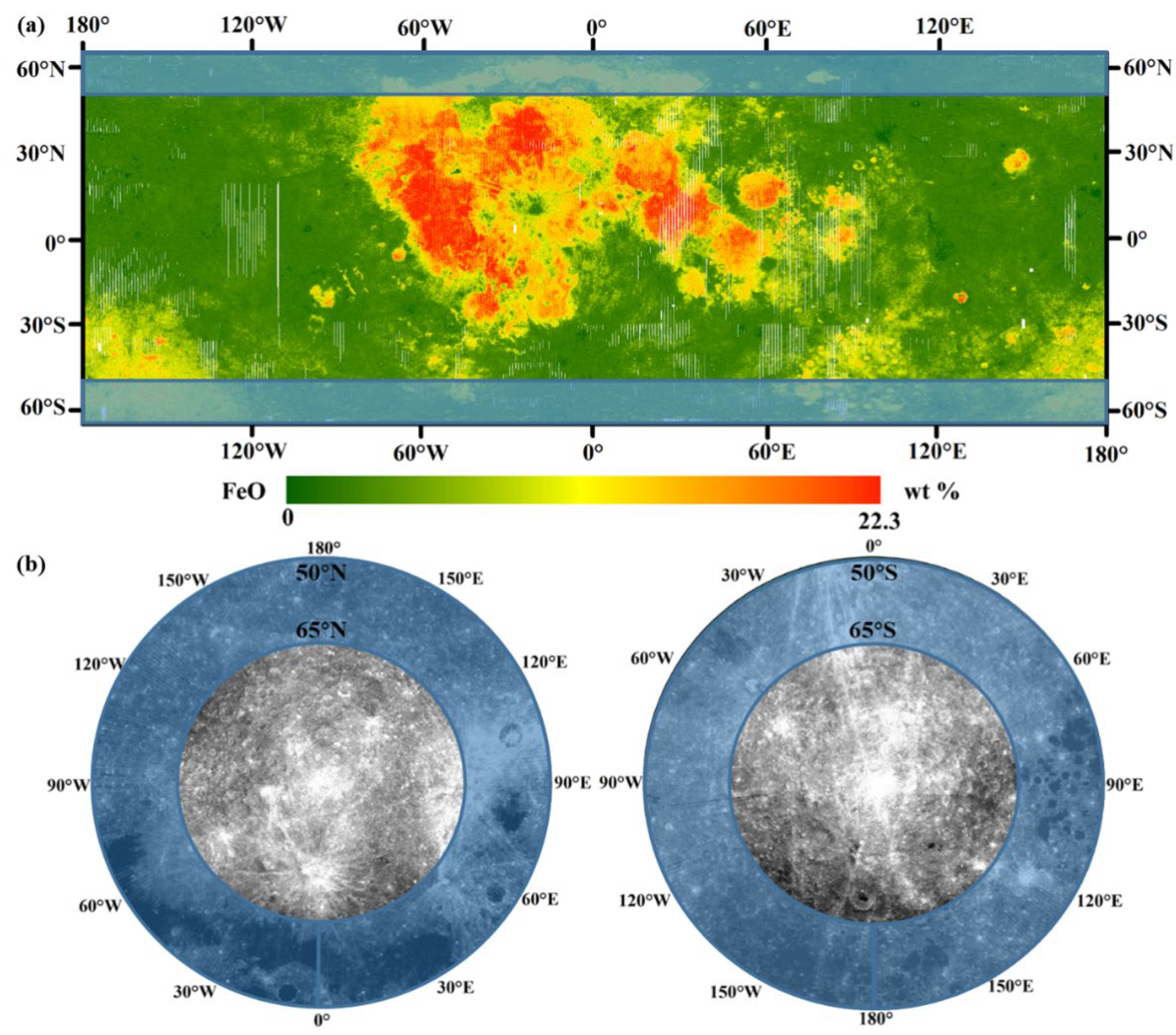
Figure 2.
Correlation coefficients between the reflectance of 150 bands of SP images and the abundance of each oxide at 940 sample data points.
Figure 2.
Correlation coefficients between the reflectance of 150 bands of SP images and the abundance of each oxide at 940 sample data points.
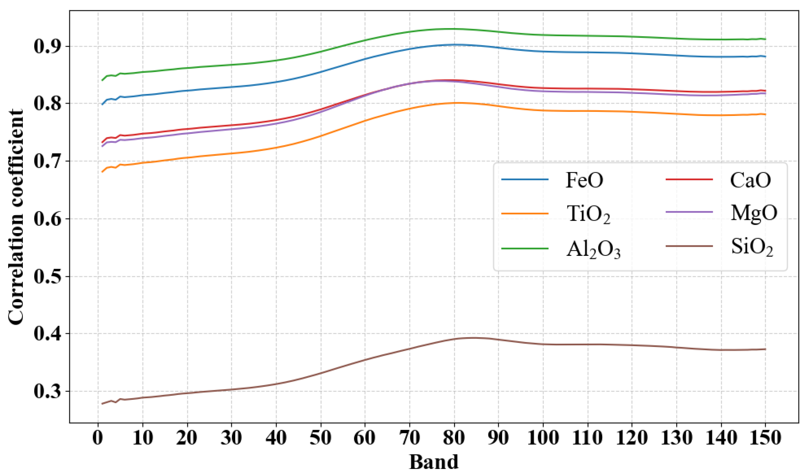
Figure 3.
1D-CNN architecture for inverting six major oxides in the lunar north and south polar regions.
Figure 3.
1D-CNN architecture for inverting six major oxides in the lunar north and south polar regions.
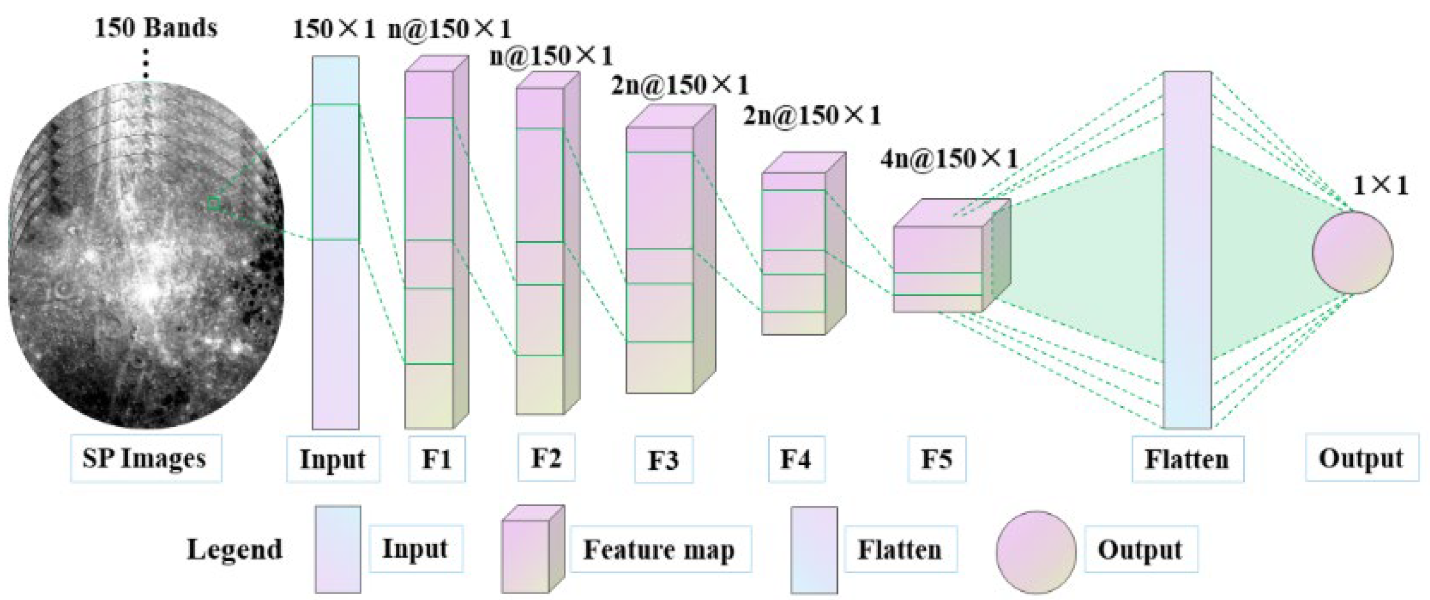
Figure 4.
Scatter plots of the abundance of each oxide predicted by the 1D-CNN model under the optimal configuration versus the measured one (in units of wt.%) at all 940 sample points.
Figure 4.
Scatter plots of the abundance of each oxide predicted by the 1D-CNN model under the optimal configuration versus the measured one (in units of wt.%) at all 940 sample points.
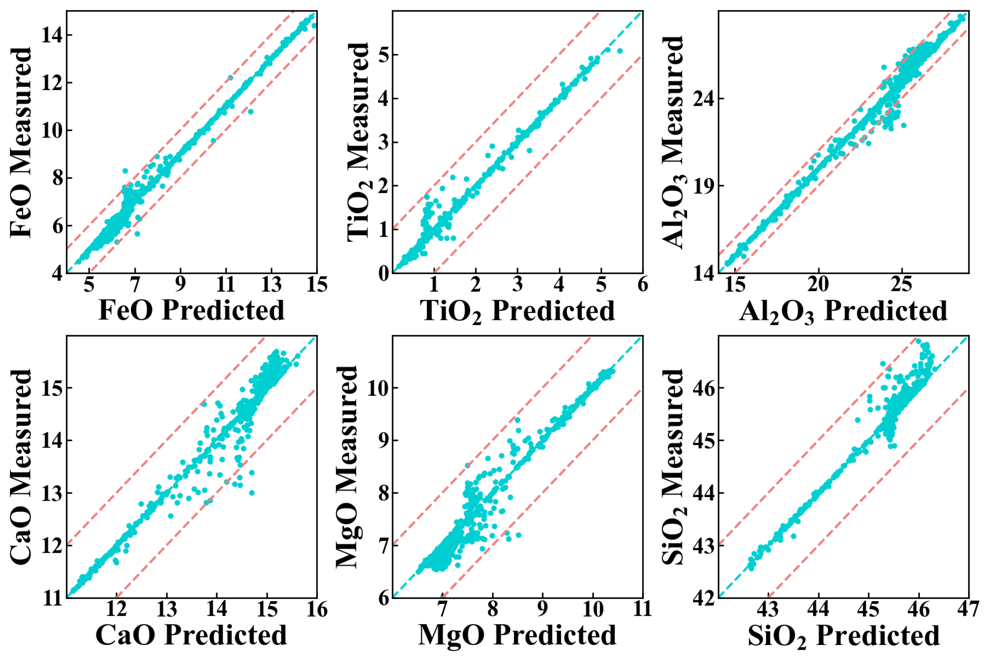
Figure 5.
Distribution of FeO inverted by the 1D-CNN model in the north (a) and south (b) polar regions.
Figure 5.
Distribution of FeO inverted by the 1D-CNN model in the north (a) and south (b) polar regions.
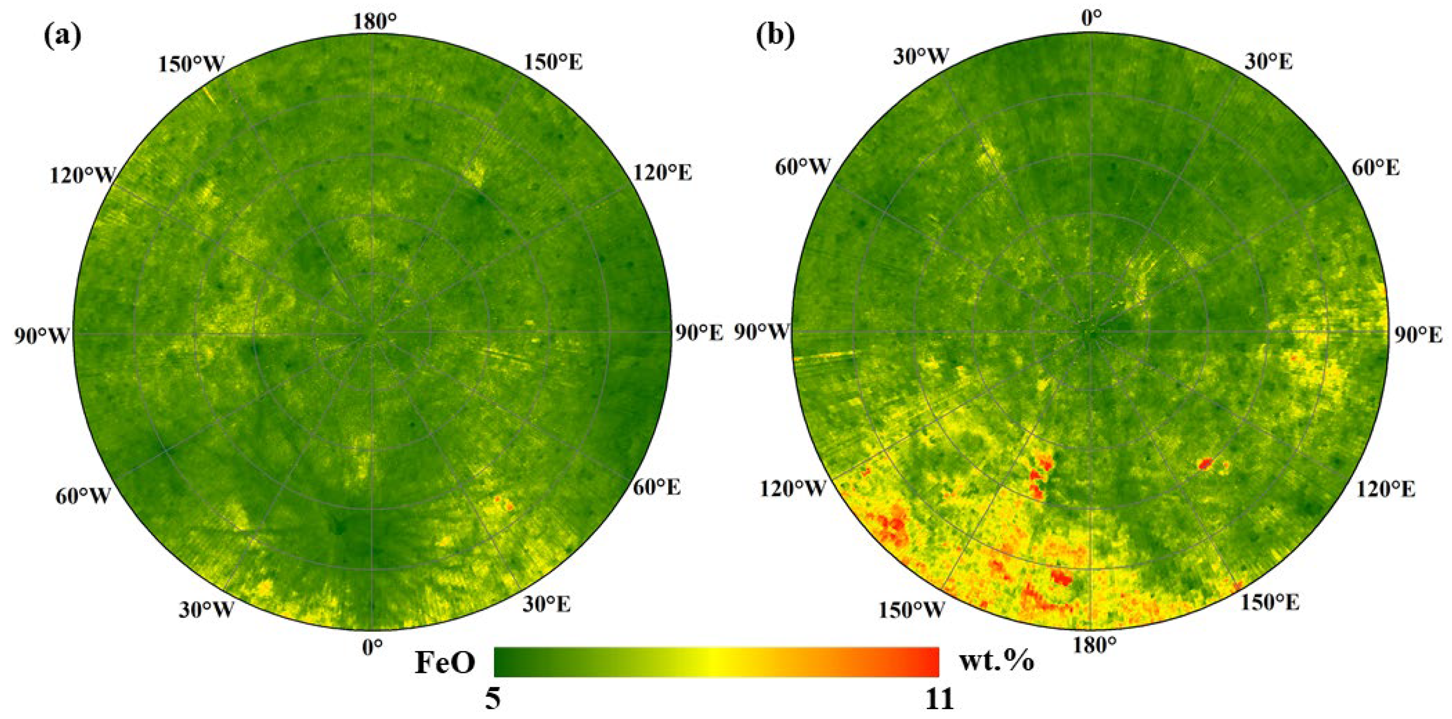
Figure 6.
Distribution of FeO inverted by Lemelin et al. (2022) in the north (a) and south (b) polar regions.
Figure 6.
Distribution of FeO inverted by Lemelin et al. (2022) in the north (a) and south (b) polar regions.
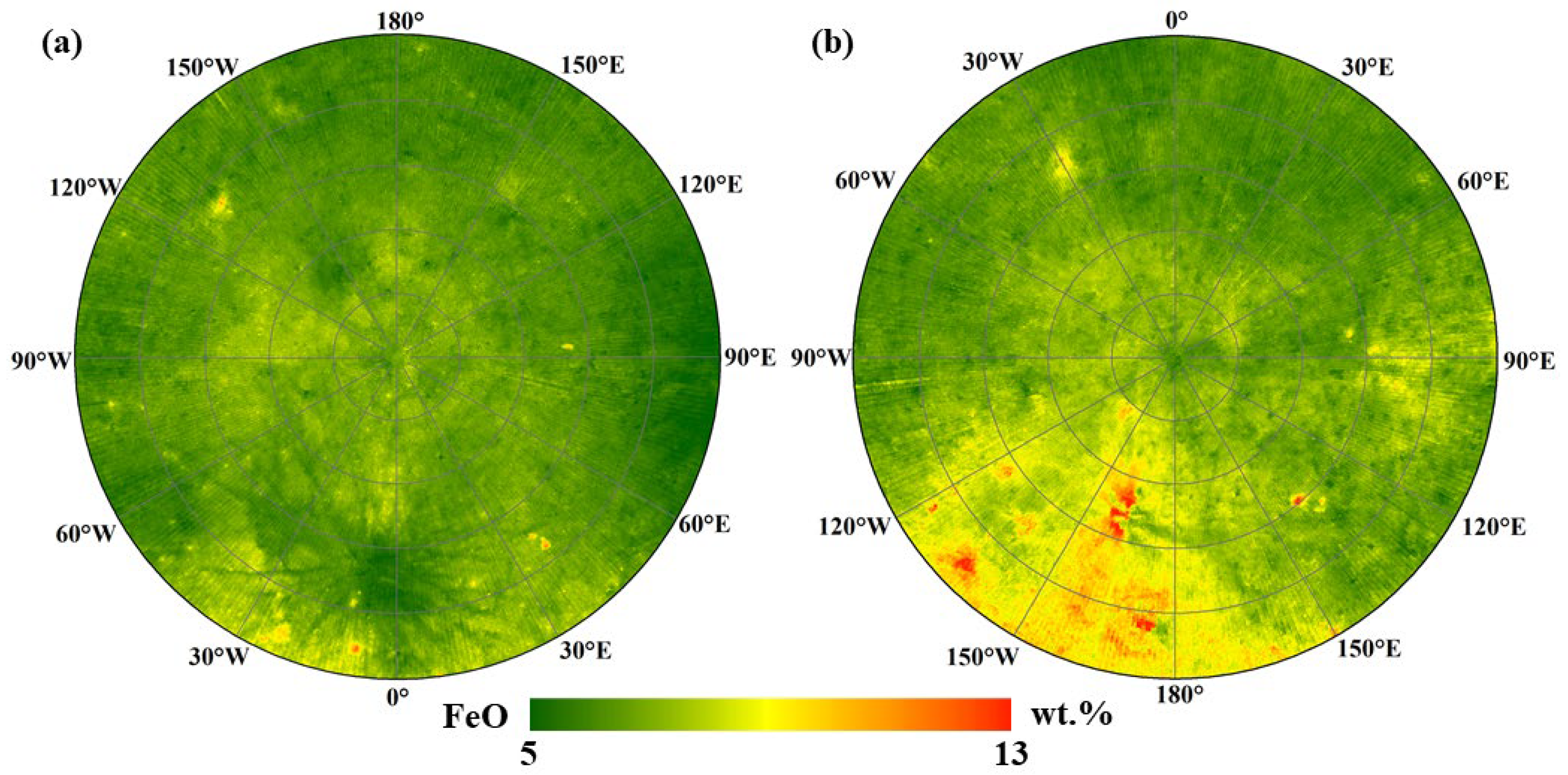
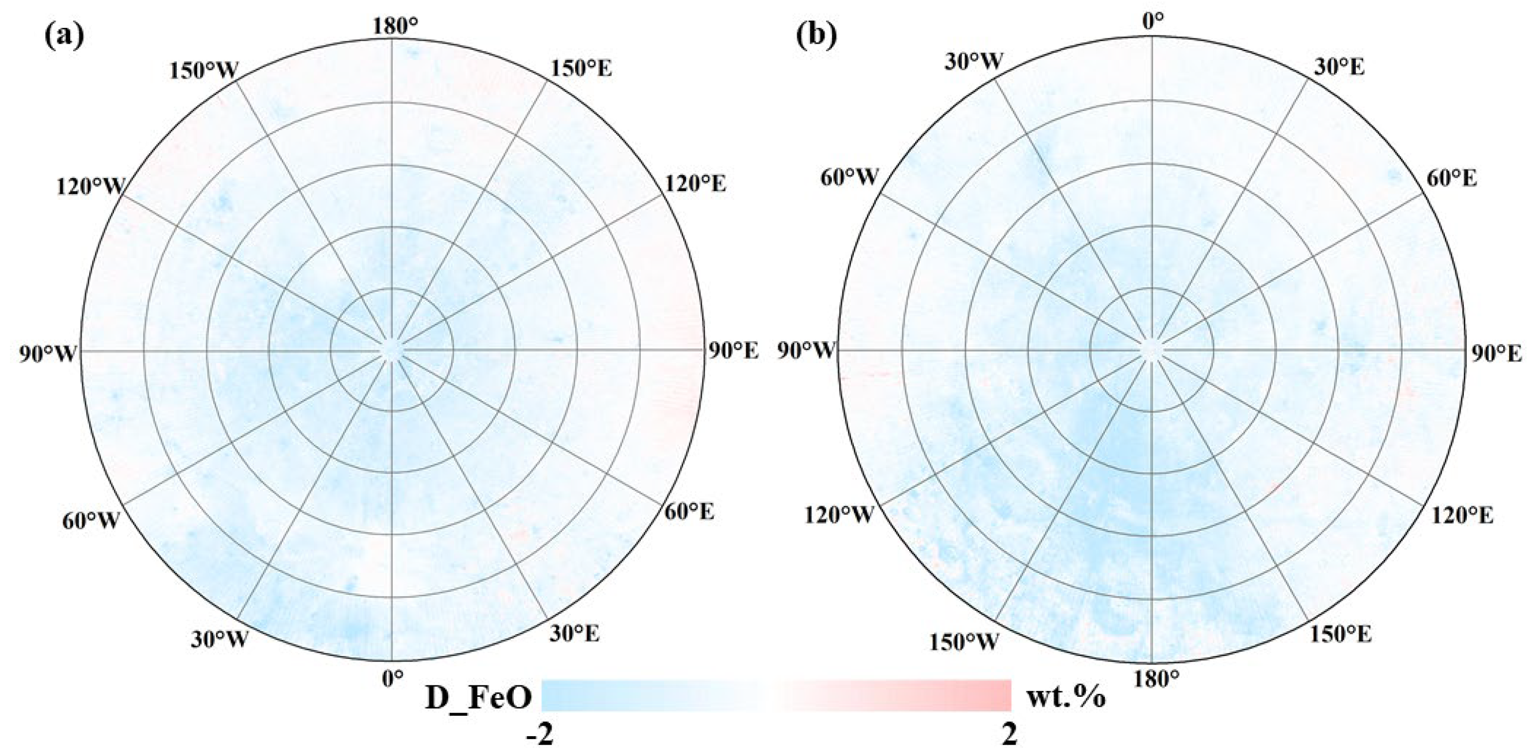
Figure 8.
Distribution of Al2O3 inverted by the 1D-CNN model in the north (a) and south (b) polar regions.
Figure 8.
Distribution of Al2O3 inverted by the 1D-CNN model in the north (a) and south (b) polar regions.
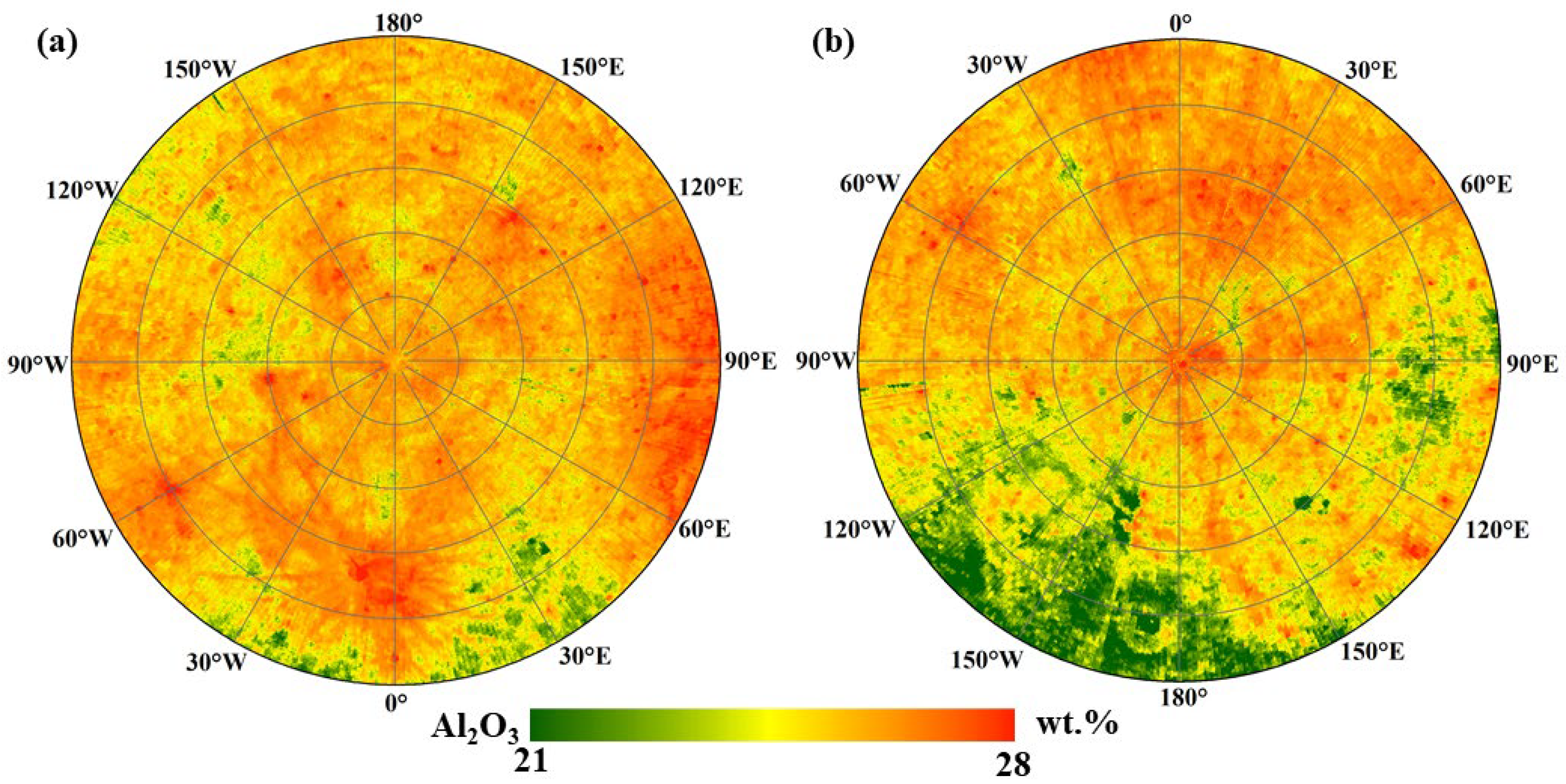
Figure 9.
Distributions of (a) TiO2, (b) CaO, (c) MgO, and (d) SiO2 inverted by the 1D-CNN model in the north (N) and south (S) polar regions.
Figure 9.
Distributions of (a) TiO2, (b) CaO, (c) MgO, and (d) SiO2 inverted by the 1D-CNN model in the north (N) and south (S) polar regions.
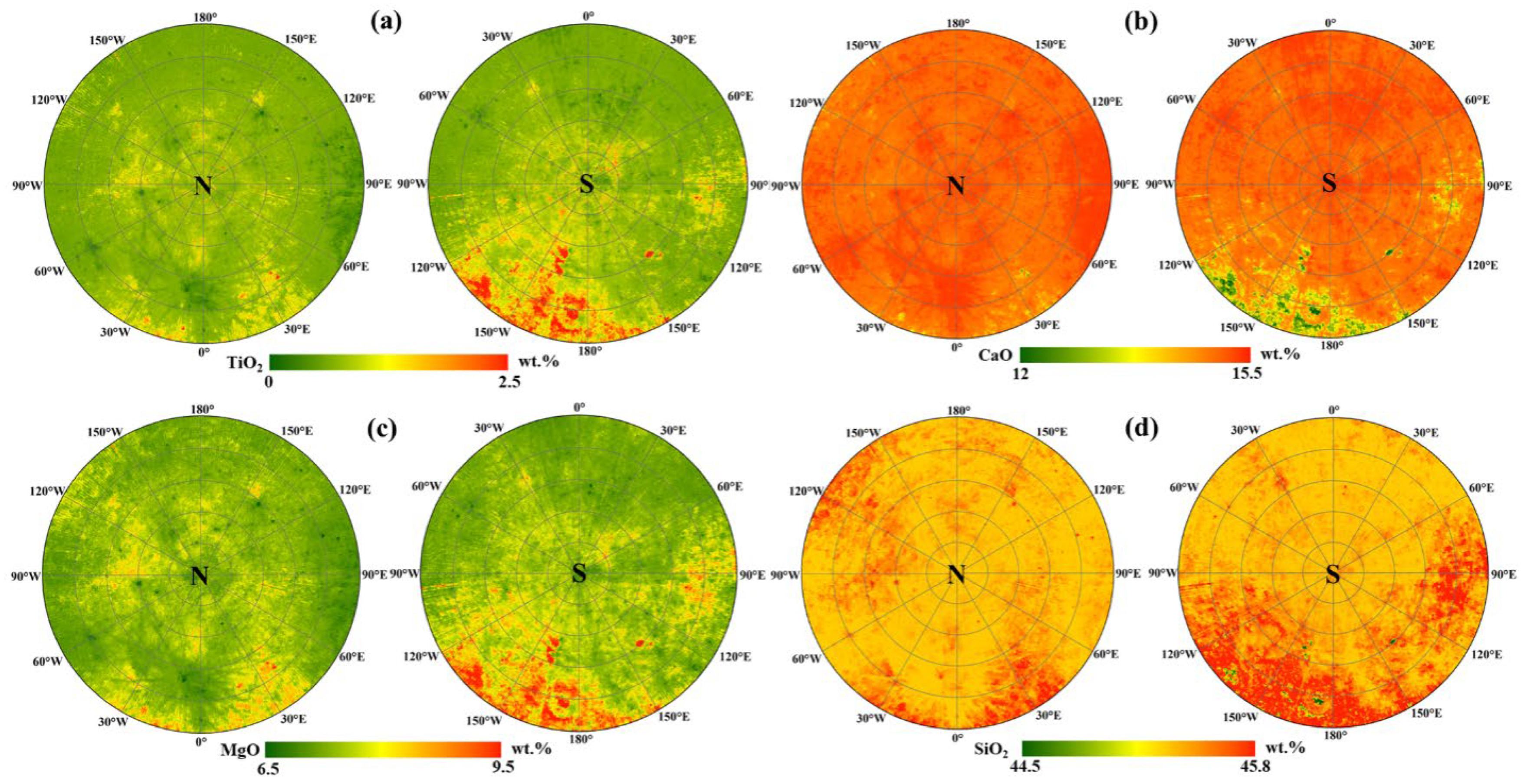
Figure 10.
FeO distributions for Regions A (upper row) and B (bottom row). The first column (a, d) is from Bian et al. (2025); The second column (b, e) is from 1D-CNN inversion; The last column (c, f) is the difference between the first two columns in the same row.
Figure 10.
FeO distributions for Regions A (upper row) and B (bottom row). The first column (a, d) is from Bian et al. (2025); The second column (b, e) is from 1D-CNN inversion; The last column (c, f) is the difference between the first two columns in the same row.
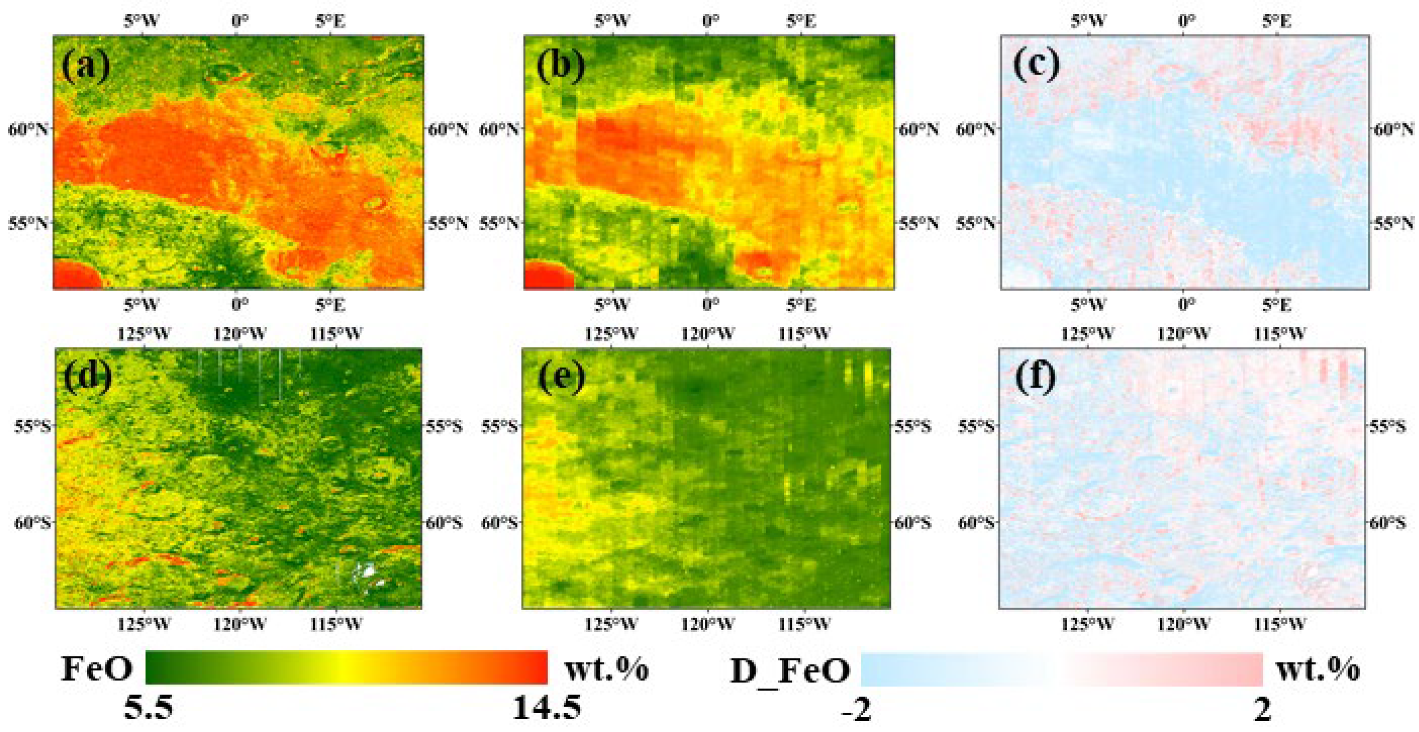
Figure 11.
Al₂O₃ distributions for Regions A (upper row) and B (bottom row). The first column (a, d) is from Bian et al. (2025); The second column (b, e) is from 1D-CNN inversion; The last column (c, f) is the difference between the first two columns in the same row.
Figure 11.
Al₂O₃ distributions for Regions A (upper row) and B (bottom row). The first column (a, d) is from Bian et al. (2025); The second column (b, e) is from 1D-CNN inversion; The last column (c, f) is the difference between the first two columns in the same row.

Figure 12.
TiO₂ distributions for Regions A (upper row) and B (bottom row). The first column (a, d) is from Bian et al. (2025); The second column (b, e) is from 1D-CNN inversion; The last column (c, f) is the difference between the first two columns in the same row.
Figure 12.
TiO₂ distributions for Regions A (upper row) and B (bottom row). The first column (a, d) is from Bian et al. (2025); The second column (b, e) is from 1D-CNN inversion; The last column (c, f) is the difference between the first two columns in the same row.
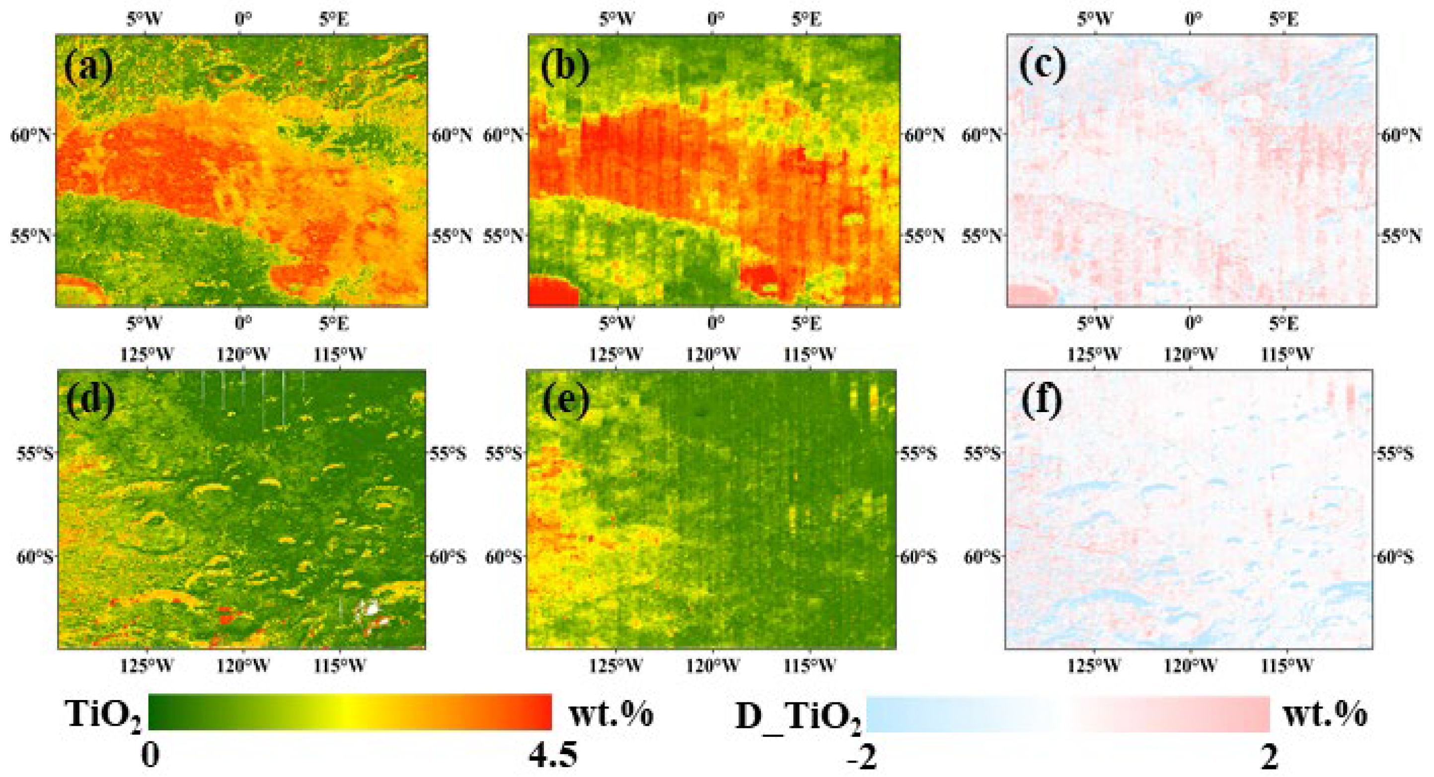
Figure 13.
Distribution of CaO (I), SiO₂ (II), and MgO (III) for Regions A (upper row) and B (bottom row). The first column (a, d) is from Bian et al. (2025); The second column (b, e) is from 1D-CNN inversion; The last column (c, f) is the difference between the first two columns in the same row.
Figure 13.
Distribution of CaO (I), SiO₂ (II), and MgO (III) for Regions A (upper row) and B (bottom row). The first column (a, d) is from Bian et al. (2025); The second column (b, e) is from 1D-CNN inversion; The last column (c, f) is the difference between the first two columns in the same row.
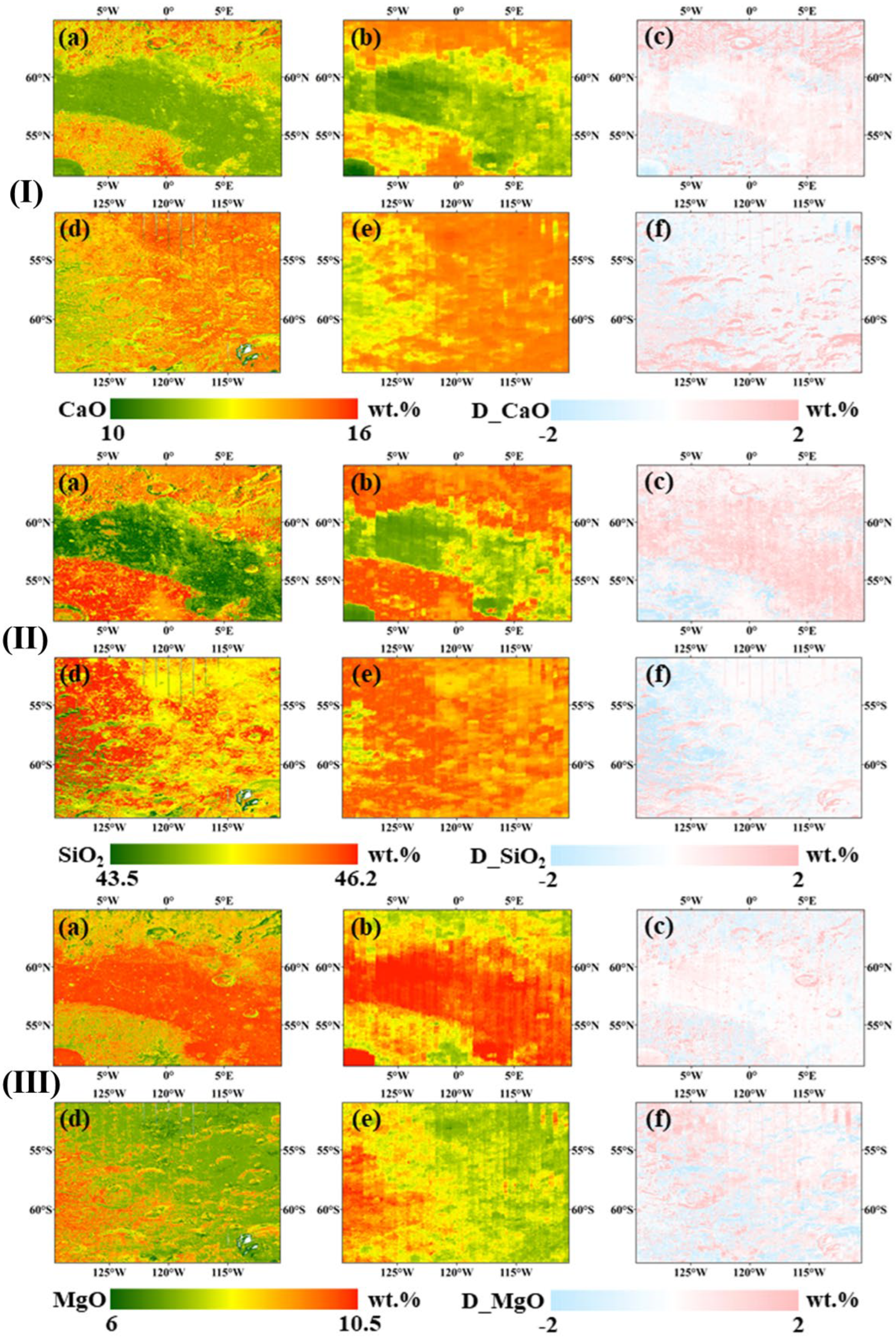
Figure 14.
Distribution of Mg# derived from FeO and MgO abundances inverted by the 1D-CNN models in the north (a) and south (b) polar regions.
Figure 14.
Distribution of Mg# derived from FeO and MgO abundances inverted by the 1D-CNN models in the north (a) and south (b) polar regions.
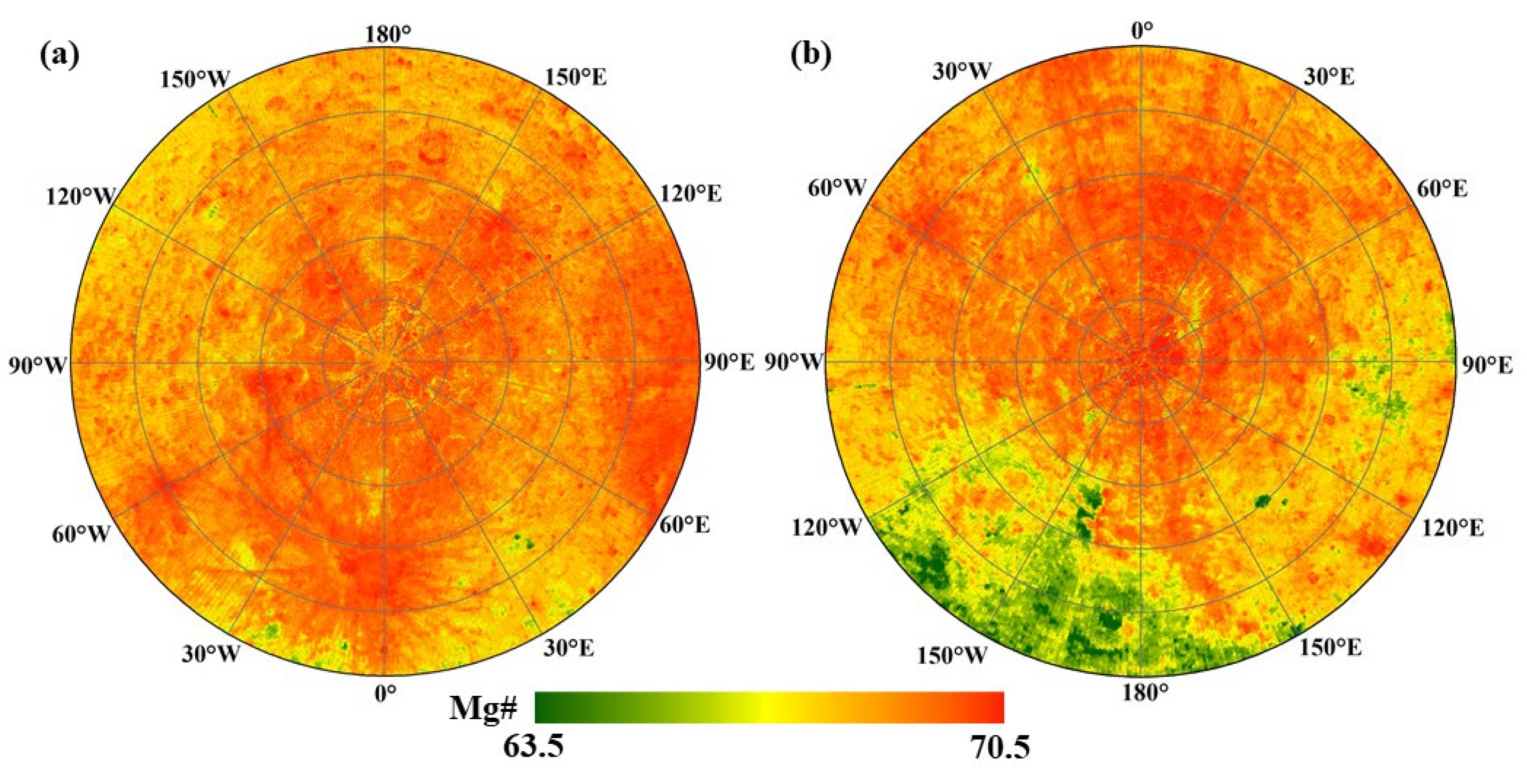
Figure 15.
Spatial distribution of nine candidate landing regions for the Artemis Ⅲ mission.
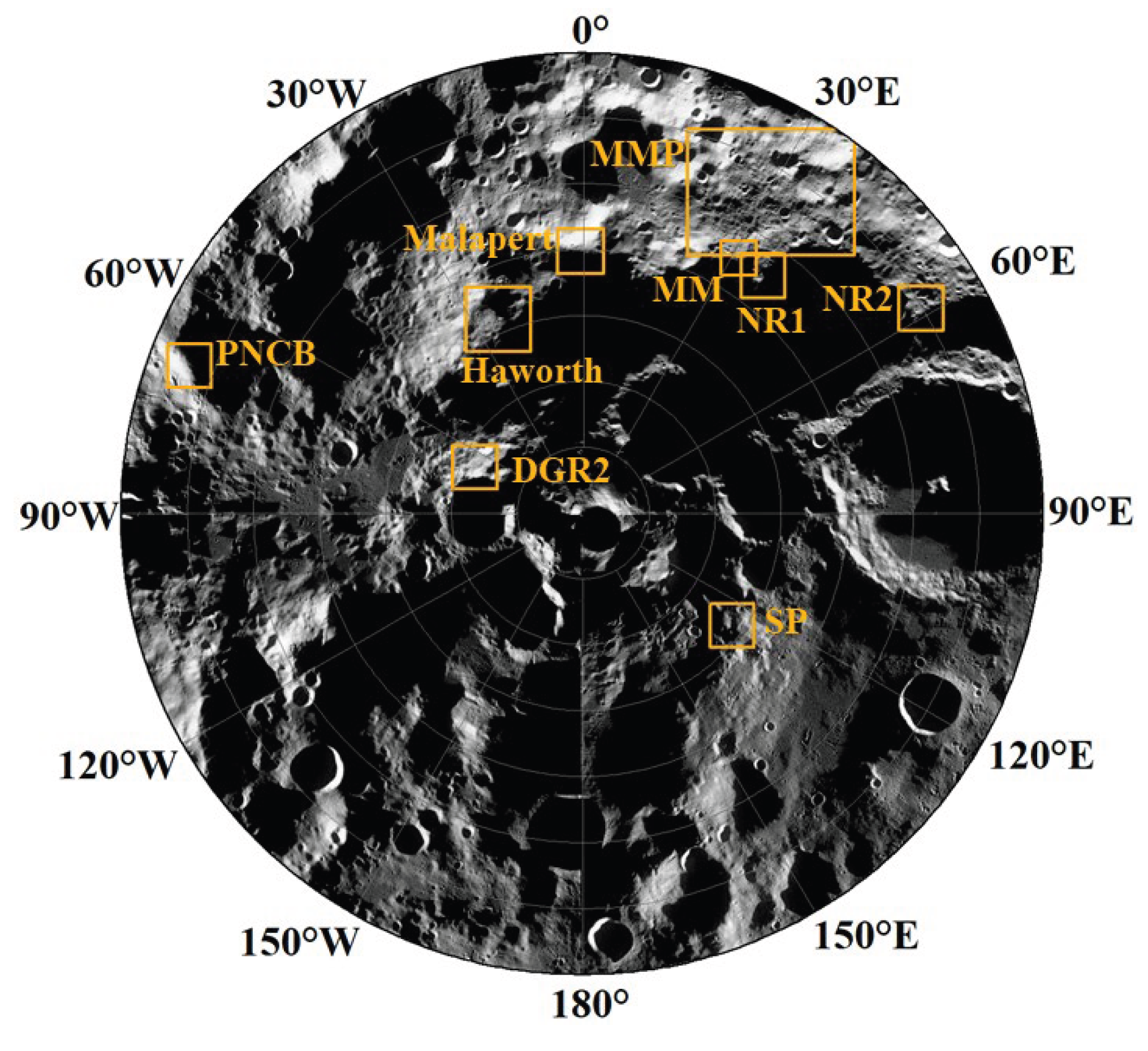

Table 1.
Performance of models resulting from different numbers of channels for each convolutional block in the case of fixed learning rate.
Table 1.
Performance of models resulting from different numbers of channels for each convolutional block in the case of fixed learning rate.
| Channel | Metric | FeO | TiO2 | Al2O3 | CaO | MgO | SiO2 |
|---|---|---|---|---|---|---|---|
| n=16 | R2 | 0.989 | 0.957 | 0.978 | 0.940 | 0.940 | 0.865 |
| RMSE | 0.263 | 0.233 | 0.485 | 0.306 | 0.283 | 0.254 | |
| n=32 | R2 | 0.994 | 0.980 | 0.985 | 0.958 | 0.941 | 0.948 |
| RMSE | 0.187 | 0.157 | 0.402 | 0.256 | 0.282 | 0.158 | |
| n=64 | R2 | 0.992 | 0.978 | 0.980 | 0.951 | 0.931 | 0.938 |
| RMSE | 0.215 | 0.167 | 0.469 | 0.275 | 0.305 | 0.172 |
Table 2.
Performance of models resulting from different learning rates for each convolutional block in the case of fixed number (n=32) of channels.
Table 2.
Performance of models resulting from different learning rates for each convolutional block in the case of fixed number (n=32) of channels.
| Learning rate | Metric | FeO | TiO2 | Al2O3 | CaO | MgO | SiO2 |
|---|---|---|---|---|---|---|---|
| 0.01 | R2 | 0.991 | 0.967 | 0.982 | 0.946 | 0.927 | 0.909 |
| RMSE | 0.230 | 0.203 | 0.438 | 0.289 | 0.314 | 0.209 | |
| 0.001 | R2 | 0.994 | 0.980 | 0.985 | 0.958 | 0.941 | 0.948 |
| RMSE | 0.187 | 0.157 | 0.402 | 0.256 | 0.282 | 0.158 | |
| 0.0001 | R2 | 0.979 | 0.958 | 0.976 | 0.941 | 0.927 | 0.882 |
| RMSE | 0.357 | 0.229 | 0.512 | 0.302 | 0.315 | 0.238 |
Table 3.
Statistical results of each oxide predicted by the 1D-CNN model under the optimal configuration.
Table 3.
Statistical results of each oxide predicted by the 1D-CNN model under the optimal configuration.
| Metric | FeO | TiO2 | Al2O3 | CaO | MgO | SiO2 |
|---|---|---|---|---|---|---|
| R | 0.997 | 0.990 | 0.992 | 0.979 | 0.971 | 0.975 |
| R2 | 0.994 | 0.980 | 0.985 | 0.958 | 0.941 | 0.948 |
| MAE/wt.% | 0.083 | 0.051 | 0.158 | 0.107 | 0.143 | 0.068 |
| RMSE/wt.% | 0.187 | 0.157 | 0.402 | 0.256 | 0.282 | 0.158 |
Table 4.
Brief information on the nine candidate landing regions for the Artemis III mission.
| No. | Region | Abbreviation | Long./° | Lat./° |
|---|---|---|---|---|
| 1 | Peak Near Cabeus B | PNCB | −69.014 | −83.661 |
| 2 | Haworth | Haworth | −22.836 | −86.753 |
| 3 | Malapert Massif | Malapert | −0.125 | −85.990 |
| 4 | Mons Mouton Plateau | MMP | 29.926 | −84.232 |
| 5 | Mons Mouton | MM | 31.586 | −85.423 |
| 6 | Nobile Rim 1 | NR1 | 37.241 | −85.431 |
| 7 | Nobile Rim 2 | NR2 | 58.654 | −83.963 |
| 8 | de Gerlache Rim 2 | DGR2 | −65.421 | −88.225 |
| 9 | Slater Plain | SP | 126.134 | −87.149 |
Table 5.
Mean and STD (unit: wt.%) of each oxide abundance in each candidate landing region.
| No. | Region | FeO | STD | TiO2 | STD | Al2O3 | STD | CaO | STD | MgO | STD | SiO2 | STD | Mg# | STD |
|---|---|---|---|---|---|---|---|---|---|---|---|---|---|---|---|
| 1 | PNCB | 5.92 | 0.40 | 0.88 | 0.34 | 25.75 | 0.91 | 15.08 | 0.11 | 7.41 | 0.24 | 45.34 | 0.05 | 69.08 | 0.95 |
| 2 | Haworth | 5.77 | 0.29 | 0.90 | 0.31 | 26.05 | 0.60 | 15.12 | 0.07 | 7.40 | 0.22 | 45.34 | 0.04 | 69.57 | 0.89 |
| 3 | Malapert | 6.02 | 0.50 | 1.09 | 0.57 | 25.49 | 0.89 | 15.04 | 0.11 | 7.59 | 0.27 | 45.35 | 0.09 | 69.24 | 1.18 |
| 4 | MMP | 6.14 | 0.58 | 1.09 | 0.54 | 25.26 | 1.05 | 15.00 | 0.14 | 7.68 | 0.33 | 45.37 | 0.10 | 69.09 | 1.22 |
| 5 | MM | 5.85 | 0.30 | 0.92 | 0.28 | 25.87 | 0.62 | 15.08 | 0.05 | 7.57 | 0.18 | 45.35 | 0.03 | 69.77 | 0.86 |
| 6 | NR1 | 6.04 | 0.49 | 1.04 | 0.45 | 25.49 | 0.87 | 15.03 | 0.11 | 7.68 | 0.28 | 45.36 | 0.08 | 69.42 | 1.14 |
| 7 | NR2 | 6.11 | 0.38 | 1.01 | 0.30 | 25.28 | 0.73 | 14.99 | 0.08 | 7.70 | 0.27 | 45.38 | 0.05 | 69.21 | 0.84 |
| 8 | DGR2 | 5.84 | 0.55 | 1.07 | 0.67 | 25.94 | 0.93 | 15.12 | 0.14 | 7.43 | 0.29 | 45.34 | 0.11 | 69.44 | 1.36 |
| 9 | SP | 5.97 | 0.57 | 1.17 | 0.68 | 25.59 | 1.00 | 15.08 | 0.13 | 7.47 | 0.29 | 45.32 | 0.12 | 69.09 | 1.47 |
Disclaimer/Publisher’s Note: The statements, opinions and data contained in all publications are solely those of the individual author(s) and contributor(s) and not of MDPI and/or the editor(s). MDPI and/or the editor(s) disclaim responsibility for any injury to people or property resulting from any ideas, methods, instructions or products referred to in the content. |
© 2025 by the authors. Licensee MDPI, Basel, Switzerland. This article is an open access article distributed under the terms and conditions of the Creative Commons Attribution (CC BY) license (http://creativecommons.org/licenses/by/4.0/).
Copyright: This open access article is published under a Creative Commons CC BY 4.0 license, which permit the free download, distribution, and reuse, provided that the author and preprint are cited in any reuse.


