Submitted:
19 November 2025
Posted:
19 November 2025
You are already at the latest version
Abstract
The booming number of EVs and autonomous vehicles is driving the demand for the development of 5G and connected vehicle technologies. However, the design of compact, multi-band vehicular antennas with multiple communication standard support is complex. Traditional experience-based and parameter-sweeping approaches to antenna optimization are often inefficient and limited in scalability, while machine learning-based methods require extensive datasets, which are computationally intensive. This study proposes a microstrip planar Yagi antenna optimized for Sub-6 GHz 5G and C-V2X communication. As a way to approach antenna optimization with lower computing cost and less data, a hybrid optimization strategy is presented that combines parametric analysis and curve fitting based data visualization approaches. The proposed antenna exhibits a reflection coefficient of -31.68 dB and -29.36 dB with 700 MHz and 900 MHz bandwidths for frequencies of 3.5 GHz and 5.9 GHz, respectively. Moreover, the proposed antenna exhibits a peak gain of 7.55 dB with a size of 0.44×0.64 λ2, while achieving a peak efficiency of 90.1%. The antenna has been integrated and simulated in a model Mini Cooper to test the effectiveness of vehicular communication.
Keywords:
C-V2X
; vehicular antenna
; antenna optimization
; parametric analysis
; curve fitting
; data visualization
1. Introduction
Intelligent Transportation Systems (ITS) are evolving rapidly to support the increasing need for safer, more efficient, and environmentally friendly mobility solutions, covering a wide range of applications, such as traffic monitoring, transportation control, and autonomous driving, designed to improve overall travel experiences and address the challenges brought about by rapid urban growth. E-mobility refers to the use of electric vehicles (EVs) powered by electricity rather than fossil fuels. This is a transformative shift in transportation, driven by advancements in technology and increasing environmental concerns. This shift toward EVs contributes to cleaner air, reduced greenhouse gas emissions, and decreased dependence on oil. A recent study by Bloomberg New Energy Finance predicts that EVs will account for 57% of global new car sales by 2040 [1]. The expansion of electric and self-driving vehicles is shaping the future of transportation. All electric vehicles have created a more favorable environment for the development of self-driving vehicles. The simpler electric motors of EVs compared to combustion engines can be more easily integrated with autonomous driving systems [2].
According to Intel’s projections, deploying AVs on roads will lead to a reduction of 250 million hours of users’ commuting time annually and save over half a million lives from 2035 to 2045 in the USA alone [3]. However, integrating a growing number of autonomous vehicles onto the current infrastructure requires smarter management, and ITS is bridging the gap. By utilizing real-time data and communication between vehicles and infrastructure, ITS can optimize traffic flow, reduce congestion, and improve safety. [4] explains how ITS can reduce traffic congestion by 15-20% and accident rates by up to 60% through dynamic traffic signal control and vehicle-to-everything (V2X) communication and [5,6] highlights how vehicles share data on speed, location, and intent, which can significantly enhance the performance of self-driving cars in urban environments. According to a report by Allied Market Research, the global V2X market size was valued at $24.52 billion in 2019 and is projected to reach $157.1 billion by 2027, growing at a CAGR of 26.7% from 2020 to 2027 [7]. This growth underscores the increasing demand for advanced communication solutions in the automotive industry. Cellular Vehicle-to-Everything (C-V2X) enables direct communication between vehicles (V2V), between vehicles and infrastructure (V2I), and between vehicles and pedestrians (V2P), fostering enhanced safety, traffic efficiency, and autonomous driving capabilities. The development of efficient C-V2X antennas is crucial to support the robust and reliable communication required for vehicular applications [8]. C-V2X technology operates primarily in the 5.9 GHz frequency band, which is designated for ITS [9]. The integration of C-V2X antennas with 5G technology further amplifies their potential, offering ultra-low latency and high-speed data transfer capabilities [10]. The design of C-V2X antennas must address several key challenges, including multi-band operation, miniaturization, and integration with vehicle architecture. Antennas must be capable of handling various frequency bands used for different communication purposes, such as navigation, infotainment, and safety applications [8]. Additionally, they must be compact and conform to the aerodynamic and aesthetic requirements of modern vehicles [11].
In general, antennas can be developed by following the general guidelines and design experience [12]. However, multi-band vehicular antennas are structurally and electromagnetically involved with sensitive design parameters due to strict specifications and performance criteria [13]. Although antenna development can be informed by experience-based knowledge, this often results in suboptimal outcomes. Experience-based parameter sweeping of a few parameters at a time has remained the most often used method for fine-tuning the geometric parameters of antenna designs in order to address this [14]. However, this approach suffers from several limitations. Manual analysis of parametric results to identify optimal configurations is time-consuming and computationally intensive, often requiring a large number of full-wave electromagnetic simulations [15]. The complexity increases with the dimensionality of the design space and the nonlinear behavior of antenna performance metrics [16]. To overcome these challenges, surrogate modeling techniques have gained attention. Data-driven surrogates, such as knowledge-based, domain-constrained deep learning models, have demonstrated the ability to approximate nonlinear antenna behavior with reduced computational costs. However, constructing accurate surrogates remains difficult due to the need to capture wide parameter variations while minimizing the training effort [17]. Similarly, population-based algorithms like Particle Swarm Optimization (PSO), though effective for optimization, become prohibitively expensive when directly applied to high-fidelity electromagnetic simulations [16].
Machine learning methods have been recently introduced in the domain of electromagnetic research to accelerate the design and optimization process as presented in the studies [18,19,20,21,22,23,24,25,26,27]. To build computationally efficient surrogate models, various kinds of ML methods have been introduced, including artificial neural network (ANN) [26], gaussian process regression (GPR) [24] and support vector machines (SVM) [19]. Although these approaches are promising, they necessitate a large dataset for effective algorithm training. Moreover, the algorithms themselves must be fine-tuned for the particular antenna being evaluated. The studies [18,19,20,21,22,23,24,25,26,27] have used several hundred to several thousand data samples for accurate prediction. Full-wave electromagnetic simulations are inherently computationally costly. Full-wave electromagnetic simulations based on numerical techniques are unavoidable for a comprehensive characterization of antennas. However, this requirement of a large dataset creates a major challenge in practical implementations and is not required for simpler antenna models.
Recent advancements focus on feature-based optimization, where the antenna design problem is reformulated using response features, characteristic attributes of the antenna’s behavior, such as resonance frequencies and return loss levels. This approach reduces the complexity of the optimization landscape, allowing for more efficient surrogate construction and quicker convergence [28,29]. By concentrating on the characteristic points in the frequency response, feature-based methods enable precise control over the placement of resonances, making them especially suitable for the design of multi-band antennas [30].
This study proposes a microstrip planar Yagi antenna for Sub-6 GHz 5G and CV2X communication. The antenna covers the most widely used Sub-6 GHz 5G band, the N78 band with a center frequency of 3.5 GHz, as well as the vehicular communication band, the 5.9 GHz band. Moreover, an approach to multi-band antenna optimization has been presented, which integrates parametric studies and curve fitting with advanced data visualization techniques, offering the potential to achieve optimal results with less data for simpler antenna design and optimization.
2. Designing the Microstrip Planar Yagi Antenna
The driven element in a Yagi antenna is generally about half a wavelength in length [31]. The directors, also known as parasitic elements, are typically shorter and around 5% less than the driven element’s length. The spacing between the driven element and each director is usually about times the wavelength. To calculate the precise lengths and spacing for a specific antenna design, Equations (1)-() offer a mathematical approach to determining the optimal dimensions for Yagi antennas based on the target operating frequency [32].
where, c = Speed of light, f = Resonant Frequency, = Wavelength.
Figure 1 illustrates the reflection coefficient of the antenna throughout the design process, while Figure 2 depicts the corresponding gain. The dipole length was determined using equations (1) to (5), leading to the design of a radiating dipole element without any directors in the initial phase (Step 1). The findings indicate that although the resonance frequency closely matched the theoretical calculations, the antenna achieved a gain of less than 6 dBi. In subsequent steps (Steps 2 to 5), directors were incrementally added, culminating in the inclusion of up to three directors. During these stages, the resonance frequency exhibited minimal variation; however, the peak gain of the antenna progressively increased to 7.6 dBi. This highlights the significant impact of the directors in terms of directional performance.
To enhance compatibility with C-V2X technology, it is beneficial for the antenna to support different types of networks. Simultaneous support for DSRC networks, cellular networks, and cellular sidelinks improves the antenna’s suitability for C-V2X applications [33,34]. The designed antenna operates at the 3.5 GHz frequency band, which is widely used for sub-6 GHz 5G networks. This ensures the compatibility of the antenna in most countries in the world [35]. However, to focus on vehicular applications, an antenna needs to operate at the 5.9 GHz frequency band for direct communication with vehicles and smart devices [36]. Tuning an antenna for a second operating frequency and optimizing its overall multi-band performance can be a complex and challenging task [37]. To achieve multi-band performance, a data visualization-based technique has been used in this study, which includes parametric analysis and curve fitting.
Figure 3(a) presents the dimensions of the single-band antenna, and Figure 3(b) presents the proposed multi-band antenna. Figure 4 compares the gain reflection coefficient of the designed single-band antenna with the reflection coefficient of the proposed multi-band antenna after optimization. Whereas Figure 5 compares the realized gain of both antennas. The optimization method and detailed results of the antenna have been discussed in the following sections.
3. Optimization of the Microstrip Planar Yagi Antenna
In order to provide effective and efficient signal transmission and reception, the optimization of an antenna is a critical step. An antenna is usually optimized by a series of systematic processes with the aim of achieving the desired performance through fine-tuning the antenna’s design parameters [38]. Initially, a parametric study has been carried out, making use of the directors’ length and spacing as the key parameters. Curve fitting techniques have been used for the obtained data after an adequate amount of data had been collected through a parametric study. In order to detect patterns and correlations and make more accurate adjustments to the antenna parameters, fitted curves created a visual representation of the data. Finally, the optimized antenna was validated by inspecting the surface current distribution of the antenna. Through these steps, the antenna’s resonance has been optimized for dual-band operation and fine-tuned to provide optimal performance for its intended application. The optimization methodology followed in this study has been illustrated in Figure 6, and the results of the proposed antenna are presented and validated in Section 4.
3.1. Parametric Analysis of the Single-Band Antenna
Parametric studies aid in performance optimization and a more thorough comprehension of key elements in numerous kinds of communication systems. An investigation can be carried out to examine how changes to key elements reflect on the performance of the antenna. By systematically varying different parameters, such as the antenna’s dimensions, shape, material properties, and feeding mechanisms, it can be analyzed how these changes affect the key performance metrics like resonance, bandwidth, gain, radiation pattern, efficiency, and impedance matching [39]. High-performance antennas for applications can be developed by using parametric studies, and the best design configurations that satisfy specific performance requirements can be determined [40]. Parametric studies aid in the development of antenna designs that can operate efficiently across multiple frequency bands and support emerging communication standards like 5G and C-V2X.
Directors and dipoles are the two primary radiating components of a Yagi antenna, where the dipole functions as the driving element, and the directors serve as parasitic elements. Figure 1 and Figure 2 illustrate a marked improvement in the antenna’s resonance frequency and gain with the progressively increased number of directors. This enhancement is evidenced by the shift in resonance frequency towards the desired range and a corresponding increase in gain. The data suggest that the systematic addition of directors leads to more efficient radiation patterns and improved overall antenna performance. Consequently, directors have been selected as the optimal components for multi-band optimization of the antenna.
The impact of varying parameter values for D1_L of the studied antenna has been analyzed in Figure 7, ranging from 8.10 mm to 20.15 mm. Although the first resonance frequency () was mostly constant at 3.5 GHz, the reflection coefficient shows some considerable variation, starting at -26.5 dB for the smallest value of D1_L, 8.10 mm, and peaking at -39.1 dB for a D1_L of 16.20 mm, before dropping to -19.6 dB for the largest value of D1_L, 20.15 mm. The bandwidth initially increases from 350 MHz to 700 MHz, and holds a similar amount of bandwidth for the next D1_L increment, before slightly decreasing to 580 MHz for the largest D1_L. For the second resonance frequency(), the frequency response is less consistent, and only a resonance could be found with two values of D1_L, which are 12.15 mm and 16.20 mm. At 12.15 mm, the second resonance frequency () is 5.9 GHz with a reflection coefficient of -22 dB and a bandwidth of 900 MHz. At 16.20 mm, the second resonance frequency () is 4.9 GHz with a decreased reflection coefficient of -19.6 dB and a significant bandwidth decrease to 160 MHz. This analysis signifies that D1_L influences the reflection coefficient and bandwidth of the first resonance frequency (). Also indicates that the choice of the length of D1 is crucial for the second resonance (), as only a certain length introduces a response in the second intended frequency band.
The impact of varying parameter values for D1_S of the studied antenna has been analyzed in Figure 8. The D1_S values range from 2.03 mm to 4.05 mm. The first resonance () of the antenna was mostly similar, with resonance around 3.5 GHz, and reflection coefficient around -30 dB, but the impact on bandwidth is much more noticeable. While D1_S is between 2.03 mm and 2.94 mm, bandwidth stays around 300 MHz and increases to 700 MHz for the last two values, 3.44 mm and 4.05 mm. For the second resonance (), as the value of D1_S increases, the resonance frequency decreases from 6.18 GHz to 5.8 GHz. The reflection coefficient also shows some variation, peaking at -33.1 dB for D1_S of 2.94 mm, and then dropping to -25.6 dB for the highest D1_S value. The bandwidth of the second resonance increases with the increasing D1_S value, starting at 375 MHz and reaching up to 900 MHz. This analysis indicates that varying the D1_S value significantly impacts the reflection coefficient and bandwidth of the antenna across both frequency bands.
The impact of varying parameter values for D2_L of the studied antenna has been analyzed in Figure 9, ranging from 10.13 mm to 26.33 mm. For the first resonance frequency (), the resonance remains relatively stable around 3.5 GHz, except for the highest value of D2_L, which is 26.33 mm, where resonance is unavailable. The trend in the reflection coefficient and bandwidth shows improvement with increasing D2_L except for the highest value. The reflection coefficient starts from -23.4 dB and reaches a maximum of -37.5 dB, and the bandwidth of the first resonance frequency () also shows improvement from 280 MHz to 700 MHz at D2_L = 18.23 mm, but decreases and becomes unavailable with further increment of D2_L. For the second resonance frequency (), the resonance is unavailable while D2_L is 10.13, but as D2_L increases, the frequency response shows a deviation from 6.0 GHz to 5.75 GHz. The reflection coefficient of the second resonance frequency () varies significantly, peaking at 45 dB for the highest D2_L value. The bandwidth shows a consistent increase, reaching up to 1000 MHz at D2_L = 26.33 mm. This analysis reveals that when the value of D2_L is 10.13 mm and 26.33 mm, the antenna only resonates at a single frequency band, either at the 3.5 GHz band or the 5.9 GHz band. This indicates that for dual-band frequency response, the value of D2_L should be between 10.13 mm and 26.33 mm. Also, adjusting the D2_L value can significantly influence both the reflection coefficient and the bandwidth.
The impact of varying parameter values for D2_S of the studied antenna has been analyzed in Figure 10, ranging from 4.05 mm to 8.91 mm. The frequency response of the first resonance frequency () spans from 3.4 GHz to 3.51 GHz. The reflection coefficient for the first resonance frequency () improves with increasing D2_S, starting from -20 dB and reaching up to -32.2 dB. The bandwidth of the first resonance frequency () also shows an increasing trend beginning at 260 MHz and peaking at 700 MHz before decreasing to 650 MHz for the highest value of D2_S. For the second resonance frequency (), as D2_S increases, the frequency shows a slight deviation starting from 6.18 GHz to 5.84 GHz. The reflection coefficient of the second resonance frequency () exhibits significant improvement, particularly for the D2_S values of 6.48 mm and 7.70 mm, where it reaches up to 33 dB before dropping to 27.1 dB for the highest D2_S value. The bandwidth of the second resonance frequency () gradually increases to 920 MHz from 140 MHz. This analysis highlights that changing the D2_S value notably impacts the resonance, reflection coefficient, and bandwidth of the antenna across both frequency bands.
Figure 11 explores the effect of varying D3_L values on antenna performance, with D3_L ranging from 15.19 mm to 27.34 mm. For the first resonance frequency (), the resonance frequency changes between 3.57 GHz and 3.41 GHz as D3_L increases. The reflection coefficient also shows some variation, initially decreasing from -26.3 dB to -25.5 dB, then improving to -31.8 dB, and slightly decreasing again to -27.7 dB at the highest value of D3_L. The bandwidth starts at 380 MHz for the lower D3_L values and increases to 700 MHz at 23.29 mm, and again decreases to 600 MHz for the highest value of D3_L. For the second resonance frequency (), the frequency remains relatively constant around 5.9 GHz, with minor fluctuations, but the reflection coefficient decreases gradually from -33.4 dB to -29.1 dB as D3_L increases, with a slight improvement to -29.7 dB at the highest D3_L value. The bandwidth (BW2) stays consistently around 900 MHz across all D3_L values, with minimal variation. This analysis indicates that while D3_L affects the first resonance frequency () more noticeably, its impact on the second resonance frequency ()is minimal.
Figure 12 illustrates the impact of varying D3_S values on antenna performance, where D3_S ranges from 10.13 mm to 16.20 mm. For the first resonance frequency (). The frequency remains nearly constant at around 3.5 GHz across all tested values of D3_S, but the reflection coefficient improves consistently with increasing value of D3_S, starting at -23.4 dB and reaching up to -37.5 dB for the highest D3_S value. The bandwidth of the first resonance frequency () initially stays around 250 MHz for the lower D3_S values but increases significantly to 700 MHz for the highest D3_S value, 16.20 mm. For the second resonance frequency (), the frequency, reflection coefficient, and bandwidth remain relatively consistent, with frequency around 5.9 GHz, reflection coefficient around -28 dB, and bandwidth around 900 MHz, with minor fluctuations. This analysis indicates that while the D3_S value does not drastically affect the operating frequencies, it does have some influence on the reflection coefficient and bandwidth of the first resonance frequency ().
3.2. Data Arrangement and Curve Fitting
To represent the relationship between a specific geometrical parameter and the resulting resonance frequency, consider a parameter x from the antenna’s physical geometry. The simulation process for determining the resonance frequency can be expressed as:
where,
- represents the electromagnetic simulation function that maps the geometry to a resulting frequency.
- f is the computed resonance frequency.
In the case of multi-band antennas, each resonant frequency corresponds to a specific operating band and thus requires its own functional relationship with the antenna’s geometrical parameters. Furthermore, to represent this, consider x as a geometric input parameter. For a multi-band antenna with n resonance frequencies, the simulation process can be modeled using n separate functions, as follows:
here,
- is the resonance frequency of the band,
- represents the simulation function relating the input parameter to the corresponding resonance frequency.
Moreover, now that a parametric study has been conducted over N samples of the input parameter, the dataset can be represented as:
where,
- is the value of the input parameter for the sample,
- is the simulated resonance frequency for the band at sample j.
With the parametric analysis presented in Section 3.1, a total of 128 data samples have been collected and structured as shown in Equation (8) to facilitate the optimization process. A summarized portion of this dataset is presented in Table 1.
Curve fitting is an optimization approach used to identify a mathematical expression that best aligns with a given set of data points. The process involves selecting a model with tunable parameters and adjusting those parameters to ensure the model’s output closely matches the data [41]. However, selecting a suitable model is essential, as an overly flexible function may follow random fluctuations instead of capturing the actual trend [42]. When applied correctly, curve fitting provides an effective way to represent the complex interactions between antenna parameters and their corresponding performance indicators, allowing for a more straightforward interpretation of the system’s behavior as design variables change [43]. Additionally, curve fitting can identify the most efficient operating regions within various frequency bands, thereby supporting improved antenna performance across the targeted spectrum. In this study, curve fitting has been utilized to explore trends and relationships within the dataset, estimate missing or specific values, and also make more accurate adjustments to the antenna parameters, which has helped to develop a better understanding of the underlying patterns in the data and has supported more informed decisions during the optimization of the proposed antenna design.
To predict resonance frequencies from any input x without running full simulations, polynomial curve fitting is applied to approximate each simulation function. A fitted polynomial model for each band i is defined as:
where,
- is the degree of the polynomial,
- are the polynomial coefficients for the band.
The coefficients are determined by minimizing the sum of squared residuals:
Finally, after curve fitting, it is important to assess the quality of the curve in representing the data; otherwise, the degree of the polynomial d can be adjusted to improve the fit. To evaluate the goodness-of-fit, the coefficient of determination is calculated for each band:
where, is the mean resonance frequency for band i, given by:
Once the fitted models are established, the next step is to determine the optimal value of x that achieves the desired set of target resonance frequencies . The optimization problem is formulated as follows:
subject to the constraints:
This loss function penalizes the deviation of the predicted resonance frequencies from their respective target values and is minimized to obtain the best-fit parameter value.
Figure 13 depicts the relationship between the length of Director 1, D1_L, and the antenna’s resonance frequencies, () and (). As the length of D1_L increases from 11 mm to 21 mm, the lower resonance frequency () remains relatively constant, with only minor fluctuations around 3.5 GHz, indicating low sensitivity to changes in D1_L. On the other hand, the higher resonance frequency () decreases significantly from about 6 GHz to 4.4 GHz as D1_L increases, demonstrating a strong inverse relationship between the length of Director 1 and the higher resonance frequency. This suggests that increasing D1_L brings the frequency response lower of the higher resonance frequency () while the lower resonance frequency () stays stable, which could be particularly useful for optimizing the antenna’s performance across multiple frequency bands for multi-band applications.
Polynomial relationship has been modeled for each resonance frequency () and () based on the input parameter D1_L, and the computed equations are presented in Equation (14) and Equation (15), with the constraint 11 mm 21 mm. Using the loss minimization function defined in Equation (13), the optimal value of D1_L has been computed for target resonance frequencies 3.5 GHz and 5.9 GHz. The optimization yielded a spacing of 12.38 mm for D1_L.
The relationship between the spacing of Director 1, D1_S, and the antenna’s resonance frequencies, () and (), has been presented in Figure 14. The data reveal that as D1_S increases from 2.0 mm to 4.0 mm, the lower resonance frequency () experiences a slight shift but stays around 3.5 GHz, indicating minimal sensitivity to changes in D1_S. In contrast, the higher resonance frequency () decreases significantly from around 6.2 GHz to 5.8 GHz, showing a much greater sensitivity to D1_S. The intersection of the two curves suggests a specific spacing where the two frequencies converge, which has been leveraged for optimization of the studied antenna for multi-band applications. This information is crucial for tuning the antenna’s performance across multiple bands, allowing for precise adjustments in the design to achieve optimal frequency responses.
Polynomial relationship has been modeled for each resonance frequency () and () based on the input parameter D1_S. The computed equations are presented in Equation (16) and Equation (17), with the constraint 2.0 mm 4.0 mm.
Using the loss minimization function defined in Equation (13), the optimal value of D1_S has been computed for target resonance frequencies 3.5 GHz and 5.9 GHz. The optimization yielded a spacing of 3.44 mm for D1_S.
Figure 15 illustrates how the length of Director 2, D2_L, affects the antenna’s resonance frequencies, () and (). As D2_L increases from 8 mm to 26 mm, the lower resonance frequency () remains relatively stable around 3.5 GHz, with only minor fluctuations up to 20 mm, indicating low sensitivity to D2_L between 8 mm and 20 mm and high sensitivity between 20 mm and 26 mm. The higher resonance frequency (), however, exhibits a more complex behavior. The frequency response initially increases from around 5.6 GHz to 6.1 GHz, peaks between 10 mm and 15 mm, and then decreases gradually to approximately 5.75 GHz as D2_L continues to increase. This variation indicates that D2_L has a significant impact on (), which can be fine-tuned by adjusting the length of Director 2 to achieve specific performance characteristics. The intersection and divergence of the two resonance frequencies at different points highlight the potential for optimizing the antenna’s dual-band capabilities by carefully selecting the length of D2_L. For D2_L, dual-band frequency response can be observed in two points in Figure 15; however, the value around 9.5 mm is discarded as the response is unstable in this region. Moreover, from Figure 9 this can be determined that the resonance is hardly touching the minimum boundary in that region.
Polynomial relationship has been modeled for each resonance frequency () and () based on the input parameter D2_L, and the computed equations are presented in Equation (18) and Equation (19), with the constraint 8 mm 26 mm. Using the loss minimization function defined in Equation (13), the optimal value of D2_L has been computed for target resonance frequencies 3.5 GHz and 5.9 GHz. The optimization yielded a spacing of 18.25 mm for D2_L.
The relationship between the spacing of Director 2, D2_S, and the antenna’s resonance frequencies, () and (), has been presented in Figure 16. The spacing of Director 2, D2_S, increases from 4.0 mm to 9.0 mm, and with increasing D2_S, the lower resonance frequency () shows a gradual increase from approximately 3.4 GHz to 3.51 GHz, indicating a positive correlation between D2_S and (). Conversely, the higher resonance frequency () gradually decreases slightly from around 6.1 GHz to 5.8 GHz, as D2_S increases. The curves intersect at a point where both resonance frequencies are close in value, which suggests a specific spacing that could be optimized for dual-band operation of the studied antenna. This information is critical for antenna design, where adjusting the spacing of Director 2 can be used to fine-tune the antenna’s resonance frequencies to achieve desired performance across multiple frequency bands.
Polynomial relationship has been modeled for each resonance frequency () and () based on the input parameter D2_S, and the computed equations are presented in Equation (20) and Equation (21), with the constraint 4.0 mm 9.0 mm. Using the loss minimization function defined in Equation (13), the optimal value of D2_S has been computed for target resonance frequencies 3.5 GHz and 5.9 GHz. The optimization yielded a spacing of 7.68 mm for D2_S.
Figure 17 illustrates how the length of Director 3, D3_L, affects the antenna’s resonance frequencies, () and (). As D3_L increases from 8 mm to 29 mm, the lower resonance frequency () remains relatively stable around 3.5 GHz, with only minor fluctuations, indicating low sensitivity to D3_L. The higher resonance frequency (), however, decreases initially from around 6.1 GHz towards 5.9 GHz between 8 mm and 21 mm and then decreases quickly to 5.7 GHz as D3_L continues to increase. This variation indicates that D3_L has a significant impact on (), which can be fine-tuned by adjusting the length of Director 3 to achieve specific performance characteristics. The intersection and divergence of the two resonance frequencies at different points highlight the potential for optimizing the antenna’s dual-band capabilities by carefully selecting the length of D3_L.
Polynomial relationship has been modeled for each resonance frequency () and () based on the input parameter D3_L, and the computed equations are presented in Equation (22) and Equation (23), with the constraint 8 mm 29 mm. Using the loss minimization function defined in Equation (13), the optimal value of D3_L has been computed for target resonance frequencies 3.5 GHz and 5.9 GHz. The optimization yielded a spacing of 23.48 mm for D3_L.
The relationship between the spacing of Director 3, D3_S, and the antenna’s resonance frequencies, () and (), has been presented in Figure 18. As D3_S varies from 10 mm to 16 mm, both resonance frequencies remain nearly constant. The lower resonance frequency () hovers around 3.5 GHz, while the higher resonance frequency () stays around 5.9 GHz. The stability of these frequencies across the range of D3_S indicates that the spacing of Director 3 has minimal impact on the antenna’s resonance frequency. This suggests that other parameters may be more influential in tuning the antenna’s performance, and D3_S can be adjusted within this range without significantly affecting the antenna’s resonance characteristics. However, as can be seen from Figure 12, although adjustment of D3_S has a minimal effect on resonance frequencies, but has some influence on the reflection coefficient and bandwidth of the lower resonance frequency ().
Polynomial relationship has been modeled for each resonance frequency () and () based on the input parameter D3_S, and the computed equations are presented in Equation (24) and Equation (25), with the constraint 10 mm 16 mm. Using the loss minimization function defined in Equation (13), the optimal value of D3_S has been computed for target resonance frequencies 3.5 GHz and 5.9 GHz. The optimization yielded a spacing of 15.74 mm for D3_S.
3.3. Visualization of Current Distribution
Visualizing the current distribution on an antenna is a powerful technique for identifying the components that most significantly affect the antenna’s radiation performance [44]. Areas with high current density, known as key contributors to the antenna’s far-field radiation, indicate which parts are critical for efficient energy transmission. Conversely, regions with minimal current flow may have little impact on radiation. Additionally, observing current distributions across different frequencies reveals the resonant modes being excited, aiding in the fine-tuning of multi-band or broadband characteristics [45]. By analyzing these patterns, this can be understood how modifications to components, for example, directors of the Yagi antenna, influence overall performance, enabling more optimized antenna designs.
The surface current distribution of the studied antenna has been presented in Figure 19. The maximum surface current of 51.57 A/m has been achieved for the resonance frequency of 3.5 GHz, and similarly, the peak surface current is 47.61 A/m for the 5.9 GHz resonance frequency. The analysis in Section 3.1 and Section 3.2 highlights the significant impact of the directors on the antenna’s radiation. Director 1, in particular, affects both resonance frequencies, with a more noticeable influence on the second resonance frequency, as seen in the current distribution. On the other hand, Director 3 has a minor effect on the first resonance frequency and does not impact the second resonance frequency.
4. Result Analysis of the Optimized Dual-Band Antenna
With the optimization presented in Section 3, the proposed antenna has been optimized for multi-band operation, specifically at resonance frequencies of 3.5 GHz and 5.9 GHz. The proposed antenna has been prototyped and presented in Figure 20(a), whereas Figure 20(b) presents the testing environment and measurement setup used to measure the characteristics of the proposed antenna.
The reflection coefficient is a critical parameter in wireless communication systems, representing the amount of energy that is reflected back towards the source. The reflection coefficient evaluates the match of impedance between the antenna and the feeding network or transmission line [22]. A lower reflection coefficient indicates enhanced power transfer and minimized signal reflections back to the source, which is crucial for achieving optimal antenna performance. This coefficient is often measured in decibels (dB), and the usual threshold is considered as -10 dB for efficient operation [13]. Bandwidth, on the other hand, defines the range of frequencies over which an antenna can effectively transmit and receive signals, and the bandwidth of an antenna is usually defined by the frequency range of the antenna under -10 dB threshold [14]. Figure 21 illustrates both the reflection coefficient and the operational bandwidth of the proposed antenna, demonstrating that the antenna operates across two distinct frequency bands, 3.5 GHz 5G cellular frequency and 5.9 GHz vehicular frequency. The multi-band operation is crucial for C-V2X application, and the proposed antenna presents significant capabilities in 3.5 GHz and 5.9 GHz frequency bands with a reflection coefficient of -31.68 dB and -29.36 dB, respectively. Also, the operational bandwidth of the proposed antenna is highly suitable for C-V2X application, with 700 MHz bandwidth in the 3.5 GHz frequency band, ranging from 3.3 GHz to 4.0 GHz, and 900 MHz in the 5.9 GHz frequency band, ranging from 5.2 GHz to 6.1 GHz. The measured reflection coefficient lines up closely with the simulation result, with some minor variation; however, the measurement result is presented up to 6 GHz frequency, constrained by the N9912A FieldFox RF Analyzer. Moreover, with a precise fabrication and measurement method, the gap between the simulated and measurement results can be minimized further.
In antenna systems, gain indicates the measure of how well an antenna concentrates the radiated power in a particular direction and how much the antenna enhances the power of an incoming signal toward the direction [15]. For an antenna system, achieving high gain is crucial for improving both signal transmission and reception performance. Applications that emphasize extensive signal coverage require antennas with high gain to facilitate communication over longer distances. This is particularly important for antennas used in vehicular communication systems, where substantial gain is essential for effective operation. The gain of the antenna is measured in units of decibels isotropic (dBi). Efficiency in antenna systems denotes the ability of the antenna to convert input power into radiated signals effectively. Antennas with higher efficiency are able to transform a greater portion of the input power into a usable radiated signal, thereby minimizing power losses.
The proposed antenna demonstrates peak gain and radiation performance across the targeted frequency bands, while also sustaining a consistent level of gain throughout the operational bandwidth, as illustrated in Figure 22. Specifically, the antenna achieves a peak gain of 7.55 dBi in the 3.5 GHz frequency band and 4.45 dBi in the 5.9 GHz frequency band. Moreover, the peak efficiency attained is 90.1% at 3.5 GHz and 78.4% at 5.9 GHz. These results indicate that the antenna not only exhibits high gains but also maintains efficient radiation in both frequency bands, which is crucial for vehicular applications.
Three-dimensional radiation and absorption patterns of an antenna system are represented by the radiation pattern. The radiation pattern is considered a crucial antenna parameter as this measures the directional radiation capabilities. Figure 23 illustrates a 2D normalized radiation pattern of the proposed antenna’s electric field (E-field) radiation across various azimuth and elevation angles, providing a visual representation of the antenna’s directional characteristics. The orientation of the antenna and the respective antenna planes are denoted with XZ, YZ, and XY axis marks. Moreover, the sectional view of the antenna has also been illustrated with the radiation pattern. Figure 23(a) depicts the radiation pattern of 3.5 GHz resonance frequency, whereas Figure 23(b) depicts the radiation pattern of 5.9 GHz resonance frequency. The polar plot is centered around the origin, with various concentric circles representing different levels of radiation intensity. The main lobe, indicating the direction of maximum radiation, is prominently shown, while smaller side lobes and nulls are visible, indicating areas of reduced or minimal radiation.
The E-field pattern for the 3.5 GHz frequency has achieved a lobe magnitude of 10.4 dB(V/m) at in XZ plane, 21.6 dB(V/m) at in YZ plane, and 21.6 dB(V/m) at in XY plane. Furthermore, for the 5.9 GHz frequency, the lobe magnitude achieved is 18 dB(V/m) at in XZ plane, 18.7 dB(V/m) at in YZ plane, and 15.3 dB(V/m) at in XY plane.
5. 3D Radiation Pattern of the Proposed Antenna with Vehicle Integration
The authors in [46] have presented CAD-based vehicle models optimized for electromagnetic simulations. To test the effectiveness of the optimized antenna while installed on vehicles, the antenna has been simulated with a 3D Mini Cooper car model. Figure 24 depicts the antenna installed on the dashboard of a Mini Cooper, and the results have been presented in Figure 25. The radiation for a frequency of 3.5 GHz is shown in Figure 25(a), where this can be seen that the primary lobe is directed outward and radiating in the car’s front direction, which is suitable for effective communication with cellular base stations. Moreover, Figure 25(b) presents the radiation for a frequency of 5.9 GHz, where this can be observed that the lobe structure differs from the previous one and is more dispersed towards the front left and right, ensuring connectivity with nearby vehicles and devices connected to the vehicular network.
6. RLC Equivalent Circuit Model of the Optimized Dual-Band Antenna
The proposed antenna has been modeled using a distributed transmission line approach, as illustrated in Figure 26. This equivalent circuit provides an electrical representation of the antenna using a combination of basic components such as resistors, capacitors, and inductors, capturing the antenna’s impedance characteristic across the operating frequencies. The feed line is represented by a series inductor L1 and resistor R1, which are connected to ground through a capacitor C1. L2, C2, and R2 represent the dipole of the antenna, which is capacitively coupled to the director element with C6 capacitance. The director elements are modeled as (L3, C3), (L4, C4), and (L5, C5), corresponding to Director 1, Director 2, and Director 3, respectively. Each director is capacitively coupled to the subsequent director and to ground, accurately representing the mutual coupling and electromagnetic interactions within the array. Finally, the completely resembled model has been analyzed and tuned using the Advanced Design System (ADS) software.
A comparison between the simulation and the RLC equivalent circuit model reveals a strong agreement in terms of reflection coefficients, as shown in Figure 27. This alignment effectively validates the design, confirming that the RLC equivalent circuit accurately reflects the antenna’s response across both targeted frequency bands: 3.5 GHz and 5.9 GHz.
7. Comparative Analysis of the Proposed Antenna
Table 2 presents a performance comparison of the proposed antenna with recent literature to highlight the prominence. Many of the examples of vehicular antennas described in the literature mainly concentrate on the 5.9 GHz legacy vehicular frequency band [47,48]. In comparison, the antenna proposed in this study supports simultaneous operation in both 3.5 GHz (5G N78) and 5.9 GHz (C-V2X) bands. The antenna presented in [47] has achieved a high gain of 7.68 dBi; however, with a size of 1.46 ×1.46 , the gain-to-size ratio is not particularly impressive. Furthermore, while designs often sacrifice overall gain or size in order to achieve multi-band operation [49], the antenna proposed in this study demonstrates a high gain of 7.55 dBi with the size of only 0.44×0.64 . With the multi-band support and compact design with high gain, the proposed antenna is suitable for demanding applications like vehicular communication.
8. Conclusion
A microstrip planar Yagi antenna for Sub-6 GHz 5G and C-V2X communication has been designed and optimized using a data-efficient optimization method. The initial single-band antenna has been optimized for dual-band operation, with frequencies of 3.5 GHz and 5.9 GHz, respectively. The optimization process follows a hybrid method that has integrated parametric studies and curve fitting with advanced data visualization techniques to the proposed antenna with 128 data samples. The dual-band antenna showcases an impressive reflection coefficient of -31.68 dB and -29.36 dB with 700 MHz and 900 MHz bandwidths for frequencies of 3.5 GHz and 5.9 GHz, respectively. Moreover, the proposed antenna exhibits an impressive gain-to-size ratio, with a peak gain of 7.55 dB and a size of 0.44×0.64 , while achieving a peak efficiency of 90.1%. Furthermore, the proposed antenna has been integrated into the dashboard of a Mini Cooper simulation model for radiation analysis, where the antenna shows different lobe structure for 3.5 GHz and 5.9 GHz frequency bands, suitable for each application requirement. This study is constrained by the lack of a precisely constructed prototype and an advanced measurement setup, despite the simulation result having been validated through the prototype and measurement. Moreover, the resonance frequency has only been considered for optimization; thus, performance optimization considering additional parameters, such as gain and efficiency, should be included in future studies. Finally, the performance of the proposed antenna has been analyzed in comparison to the recent literature, and altogether, the proposed antenna demonstrates promising performance for 5G and C-V2X, specifically for vehicular communication.
Author Contributions
Conceptualization and writing—original draft preparation, D. Saha; writing—review, editing and supervision, I. M. Nawi;
Funding
This research is partially funded by Total Energies EP Malaysia Project Grant, cost center 015MD0-169.
Data Availability Statement
Dataset available on request from the authors.
Acknowledgments
The author expresses sincere appreciation to Vehicle4em Team for the simulation model of Mini Cooper. The authors also acknowledge the use of Artificial Intelligence (AI) tools to enhance the grammar, clarity, and formatting of this manuscript at the final stage. All ideas, analyses, and conclusions presented are entirely the authors’ own.
Conflicts of Interest
The authors declare no conflicts of interest.
References
- Finance, B.N.E. Bloomberg New Energy Finance, Electric Vehicle Outlook 2023. https://assets.bbhub.io/professional/sites/24/2431510_BNEFElectricVehicleOutlook2023_ExecSummary.pdf, 2023. [Accessed 05-06-2024].
- K, B.N.K.R.; D, P.; B, S.; E, J.R. Recent AI Applications in Electrical Vehicles for Sustainability. International Journal of Mechanical Engineering 2024, 11, 50–64. [Google Scholar] [CrossRef]
- Park, H.; Piamrat, K.; Singh, K.; Chen, H.C. Data analysis for self-driving vehicles in intelligent transportation systems. Journal of Advanced Transportation 2020, 2020, 1–2. [Google Scholar] [CrossRef]
- Elassy, M.; Al-Hattab, M.; Takruri, M.; Badawi, S. Intelligent transportation systems for sustainable smart cities. Transportation Engineering, 1002. [Google Scholar]
- Autili, M.; Chen, L.; Englund, C.; Pompilio, C.; Tivoli, M. Cooperative intelligent transport systems: Choreography-based urban traffic coordination. IEEE Transactions on Intelligent Transportation Systems 2021, 22, 2088–2099. [Google Scholar] [CrossRef]
- Loke, S.W. Cooperative automated vehicles: A review of opportunities and challenges in socially intelligent vehicles beyond networking. IEEE Transactions on Intelligent Vehicles 2019, 4, 509–518. [Google Scholar] [CrossRef]
- Research, A.M. Automotive V2X Market Size, Technology, Report 2021-2030 — alliedmarketresearch.com. https://www.alliedmarketresearch.com/automotive-v2x-market-A07120. [Accessed 28-05-2024].
- Mir, Z.H.; Dreyer, N.; Kürner, T.; Filali, F. Investigation on cellular LTE C-V2X network serving vehicular data traffic in realistic urban scenarios. Future Generation Computer Systems 2024, 161, 66–80. [Google Scholar]
- Maglogiannis, V.; Naudts, D.; Hadiwardoyo, S.; Van Den Akker, D.; Marquez-Barja, J.; Moerman, I. Experimental V2X evaluation for C-V2X and ITS-G5 technologies in a real-life highway environment. IEEE Transactions on Network and Service Management 2021, 19, 1521–1538. [Google Scholar]
- Abdel Hakeem, S.A.; Hady, A.A.; Kim, H. 5G-V2X: Standardization, architecture, use cases, network-slicing, and edge-computing. Wireless Networks 2020, 26, 6015–6041. [Google Scholar]
- Saha, D.; Nawi, I.M.; Zakariya, M. Super low profile 5G mmWave highly isolated MIMO antenna with 360∘ pattern diversity for smart city IoT and vehicular communication. Results in Engineering 2024, 24, 103209. [Google Scholar] [CrossRef]
- Weiland, T.; Timm, M.; Munteanu, I. A practical guide to 3-D simulation. IEEE microwave magazine 2008, 9, 62–75. [Google Scholar] [CrossRef]
- Alieldin, A.; Huang, Y.; Boyes, S.J.; Stanley, M.; Joseph, S.D.; Hua, Q.; Lei, D. A triple-band dual-polarized indoor base station antenna for 2G, 3G, 4G and sub-6 GHz 5G applications. IEEE Access 2018, 6, 49209–49216. [Google Scholar] [CrossRef]
- Akinsolu, M.O.; Mistry, K.K.; Liu, B.; Lazaridis, P.I.; Excell, P. Machine learning-assisted antenna design optimization: A review and the state-of-the-art. In Proceedings of the 2020 14th European conference on antennas and propagation (EuCAP). IEEE; 2020; pp. 1–5. [Google Scholar]
- Koziel, S.; Pietrenko-Dabrowska, A. Improved-efficacy EM-driven optimization of antenna structures using adaptive design specifications and variable-resolution models. IEEE Transactions on Antennas and Propagation 2023, 71, 1863–1874. [Google Scholar] [CrossRef]
- Koziel, S.; Pietrenko-Dabrowska, A. On nature-inspired design optimization of antenna structures using variable-resolution EM models. Scientific Reports 2023, 13, 8373. [Google Scholar] [CrossRef]
- Koziel, S.; Çalık, N.; Mahouti, P.; Belen, M.A. Low-cost and highly accurate behavioral modeling of antenna structures by means of knowledge-based domain-constrained deep learning surrogates. IEEE Transactions on Antennas and Propagation 2022, 71, 105–118. [Google Scholar] [CrossRef]
- Liu, Y.F.; Xiao, L.Y.; Liu, Q.H. Machine Learning-Based Design Scheme for Multifunctional Antenna Arrays with Reconfigurable Scattering Patterns. IEEE Transactions on Antennas and Propagation 2025. [Google Scholar] [CrossRef]
- Shereen, M.K.; Liu, X.; Wu, X. Support Vector Regression for Gain and S11 Prediction: a Low-Complexity Solution for Antenna Design. In Proceedings of the 2025 IEEE 20th International Symposium on Antenna Technology and Applied Electromagnetics (ANTEM). IEEE; 2025; pp. 1–4. [Google Scholar]
- Rahman, M.A.; Al-Bawri, S.S.; Larguech, S.; Alharbi, S.S.; Alsowail, S.; Jizat, N.M.; Islam, M.T. Metamaterial based tri-band compact MIMO antenna system for 5G IoT applications with machine learning performance verification. Scientific Reports 2025, 15, 22866. [Google Scholar] [CrossRef] [PubMed]
- Nakmouche, M.F.; Deslandes, D.; Nedil, M.; Gagnon, G. Machine learning-aided design of defected ground structures for PRGW-based MIMO antennas. IEEE Transactions on Antennas and Propagation 2025. [Google Scholar] [CrossRef]
- Shereen, M.K.; Liu, X.; Wu, X.; Naseem, A.; Uzair, M. Deep learning-inspired linear regression technique for accurate microstrip antenna performance analysis. In Proceedings of the 2025 4th International Conference on Electronics Representation and Algorithm (ICERA). IEEE; 2025; pp. 42–47. [Google Scholar]
- Haque, M.A.; Ahammed, M.S.; Rahaman, M.S.A.; Ahmed, M.K.; Nahin, K.H.; Sawaran Singh, N.S.; Rahman, M.A.; Jaafar, J.; Al-Bawri, S.S. High Performance Quad Port Compact MIMO Antenna for 38 GHz 5G Application with Regression Machine Learning Prediction. Journal of Infrared, Millimeter, and Terahertz Waves 2025, 46, 40. [Google Scholar] [CrossRef]
- Narayanaswamy, N.K.; Alzahrani, Y.; Penmatsa, K.K.V.; Pandey, A.; Dwivedi, A.K.; Singh, V.; Tolani, M. Machine learning aided tapered 4-port MIMO antenna for V2X communications with enhanced gain and isolation. IEEE Access 2025. [Google Scholar] [CrossRef]
- Tanti, H.A.; Datta, A.; Biswas, T.; Tripathi, A. Development of a machine learning-based radio source localization algorithm for tri-axial antenna configuration. Journal of Astrophysics and Astronomy 2025, 46, 1–10. [Google Scholar] [CrossRef]
- Gajbhiye, P.A.; Singh, S.P.; Sharma, M.K. Hybrid optimization framework for MIMO antenna design in wearable IoT applications using deep learning and bayesian method. Brazilian Journal of Physics 2025, 55, 3. [Google Scholar] [CrossRef]
- Alam, M.M.; Yusof, N.A.T.; Faudzi, A.A.M.; Tomal, M.R.I.; Haque, M.E.; Rahman, M.S. Machine learning-based approach for bandwidth and frequency prediction of circular SIW antenna. Journal of King Saud University–Engineering Sciences 2025, 37, 1–19. [Google Scholar] [CrossRef]
- Koziel, S.; Pietrenko-Dabrowska, A.; Pankiewicz, B. On accelerated metaheuristic-based electromagnetic-driven design optimization of antenna structures using response features. Electronics 2024, 13, 383. [Google Scholar] [CrossRef]
- Koziel, S.; Pietrenko-Dabrowska, A. Efficient simulation-based global antenna optimization using characteristic point method and nature-inspired metaheuristics. IEEE Transactions on Antennas and Propagation 2024. [Google Scholar] [CrossRef]
- Koziel, S.; Pietrenko-Dabrowska, A. Expedited feature-based quasi-global optimization of multi-band antenna input characteristics with jacobian variability tracking. IEEE Access 2020, 8, 83907–83915. [Google Scholar] [CrossRef]
- Yu, X.; Weeber, J.C.; Markey, L.; Arocas, J.; Bouhelier, A.; Leray, A.; des Francs, G.C. Nano antenna-assisted quantum dots emission into high-index planar waveguide. Nanotechnology 2024, 35, 265201. [Google Scholar] [CrossRef] [PubMed]
- Barbano, N. Log periodic Yagi-Uda array. IEEE Transactions on Antennas and Propagation 1966, 14, 235–238. [Google Scholar] [CrossRef]
- Rehman, A.; Valentini, R.; Cinque, E.; Di Marco, P.; Santucci, F. On the Impact of Multiple Access Interference in LTE-V2X and NR-V2X Sidelink Communications. Sensors 2023, 23, 4901. [Google Scholar] [CrossRef] [PubMed]
- Ficzere, D.; Varga, P.; Wippelhauser, A.; Hejazi, H.; Csernyava, O.; Kovács, A.; Hegedus, C. Large-Scale Cellular Vehicle-to-Everything Deployments Based on 5G—Critical Challenges, Solutions, and Vision towards 6G: A Survey. Sensors 2023, 23, 7031. [Google Scholar] [CrossRef]
- Pant, M.; Malviya, L. Design, developments, and applications of 5G antennas: a review. International journal of microwave and wireless technologies 2023, 15, 156–182. [Google Scholar] [CrossRef]
- Kihei, B.; Barclay, C.; Greaves-Taylor, J.; et al. 5.9 GHz Interference Resiliency for Connected Vehicle Equipment. Technical report, Georgia. Dept. of Transporation. Office of Performance-Based Management and …, 2023.
- Boursianis, A.D.; Papadopoulou, M.S.; Pierezan, J.; Mariani, V.C.; Coelho, L.S.; Sarigiannidis, P.; Koulouridis, S.; Goudos, S.K. Multiband patch antenna design using nature-inspired optimization method. IEEE Open journal of Antennas and Propagation 2020, 2, 151–162. [Google Scholar] [CrossRef]
- Liu, Y.F.; Chang, T.H.; Hong, M.; Wu, Z.; So, A.M.C.; Jorswieck, E.A.; Yu, W. A survey of recent advances in optimization methods for wireless communications. IEEE Journal on Selected Areas in Communications 2024. [Google Scholar] [CrossRef]
- Haque, M.A.; Zakariya, M.A.; Singh, N.S.S.; Rahman, M.A.; Paul, L.C. Parametric study of a dual-band quasi-Yagi antenna for LTE application. Bulletin of Electrical Engineering and Informatics 2023, 12, 1513–1522. [Google Scholar] [CrossRef]
- Pietrenko-Dabrowska, A.; Koziel, S. Accelerated parameter tuning of antenna structures by means of response features and principal directions. IEEE Transactions on Antennas and Propagation 2023. [Google Scholar] [CrossRef]
- Caceci, M.S.; Cacheris, W.P. Fitting curves to data. Byte 1984, 9, 340–362. [Google Scholar]
- Lever, J.; Krzywinski, M.; Altman, N. Points of significance: model selection and overfitting. Nature methods 2016, 13, 703–705. [Google Scholar] [CrossRef]
- Verma, R.K.; Srivastava, D.K. Optimization and parametric analysis of slotted microstrip antenna using particle swarm optimization and curve fitting. International Journal of Circuit Theory and Applications 2021, 49, 1868–1883. [Google Scholar] [CrossRef]
- El-Hakim, H.; Mohamed, H.A. synthesis of a multiband microstrip patch antenna for 5G wireless communications. Journal of Infrared, Millimeter, and Terahertz Waves 2023, 44, 752–768. [Google Scholar] [CrossRef]
- You, C.J.; Liu, S.H.; Zhang, J.X.; Wang, X.; Li, Q.Y.; Yin, G.Q.; Wang, Z.G. Frequency-and pattern-reconfigurable antenna array with broadband tuning and wide scanning angles. IEEE Transactions on Antennas and Propagation 2023, 71, 5398–5403. [Google Scholar] [CrossRef]
- Freschi, F.; Giaccone, L.; Cirimele, V.; Solimene, L. Vehicle4em: a collection of car models for electromagnetic simulation. In Proceedings of the Proceedings of the IEEE Wireless Power Transfer Conference and Expo (WPTCE), Rome, Italy; 2025. [Google Scholar]
- Sufian, M.A.; Hussain, N.; Abbas, A.; Lee, J.; Park, S.G.; Kim, N. Mutual coupling reduction of a circularly polarized MIMO antenna using parasitic elements and DGS for V2X communications. IEEE Access 2022, 10, 56388–56400. [Google Scholar] [CrossRef]
- Xing, X.Q.; Lu, W.J.; Ji, F.Y.; Zhu, L.; Zhu, H.B. Low-profile dual-resonant wideband backfire antenna for vehicle-to-everything applications. IEEE Transactions on Vehicular Technology 2022, 71, 8330–8340. [Google Scholar] [CrossRef]
- Virothu, S.; Anuradha, M.S. Flexible CP diversity antenna for 5G cellular Vehicle-to-Everything applications. AEU-International Journal of Electronics and Communications 2022, 152, 154248. [Google Scholar] [CrossRef]
Figure 1.
Reflection Coefficient of the Microstrip Planar Yagi Antenna at Each Step.
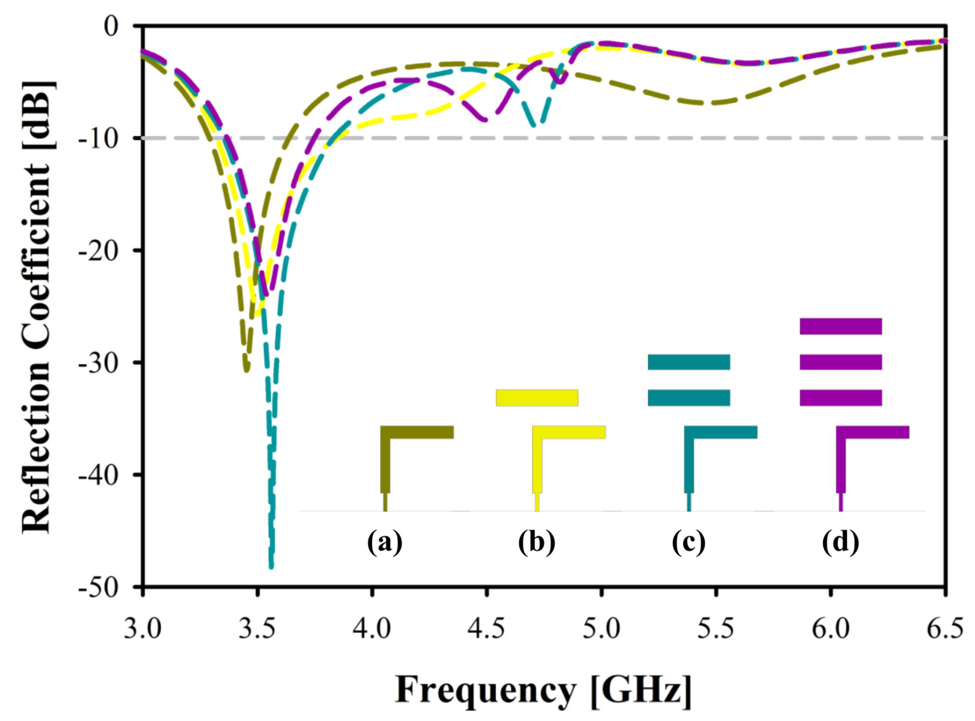
Figure 2.
Realized Gain of the Microstrip Planar Yagi Antenna at Each Step.
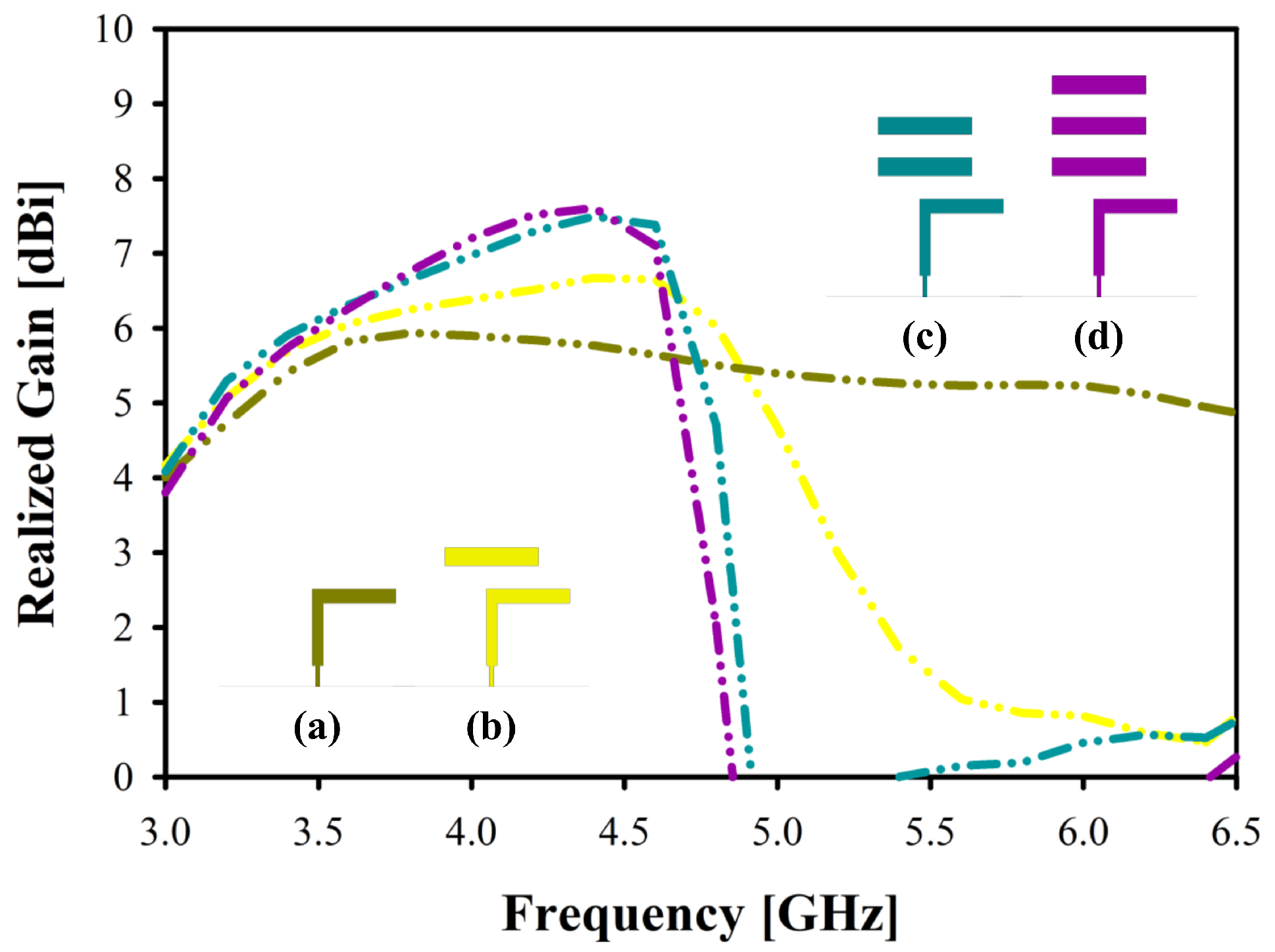
Figure 3.
Front and Back View of the Designed Microstrip Planar Yagi Antenna. (a) Initial Single-Band Antenna. (b) Proposed Dual-Band Antenna.
Figure 3.
Front and Back View of the Designed Microstrip Planar Yagi Antenna. (a) Initial Single-Band Antenna. (b) Proposed Dual-Band Antenna.
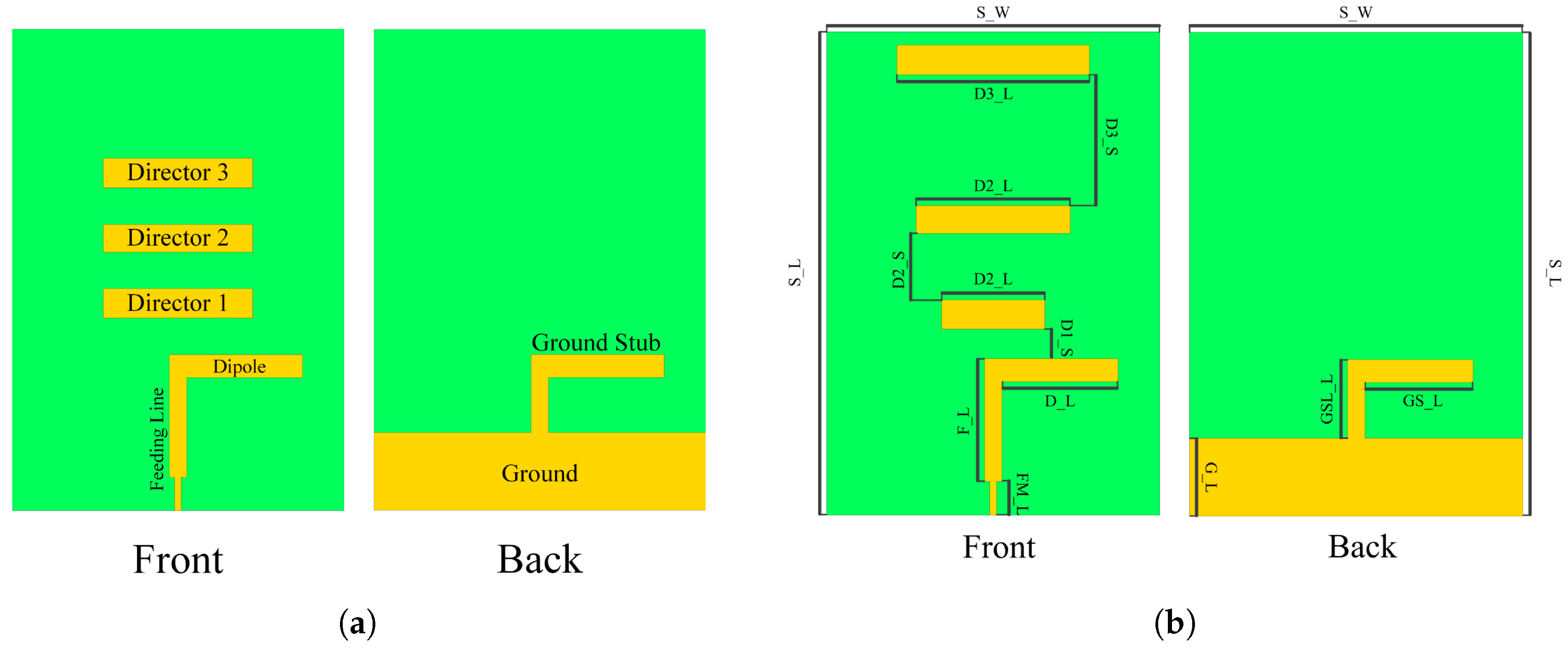
Figure 4.
Reflection Coefficient of the Single-Band Antenna and the Proposed Dual-Band Antenna.
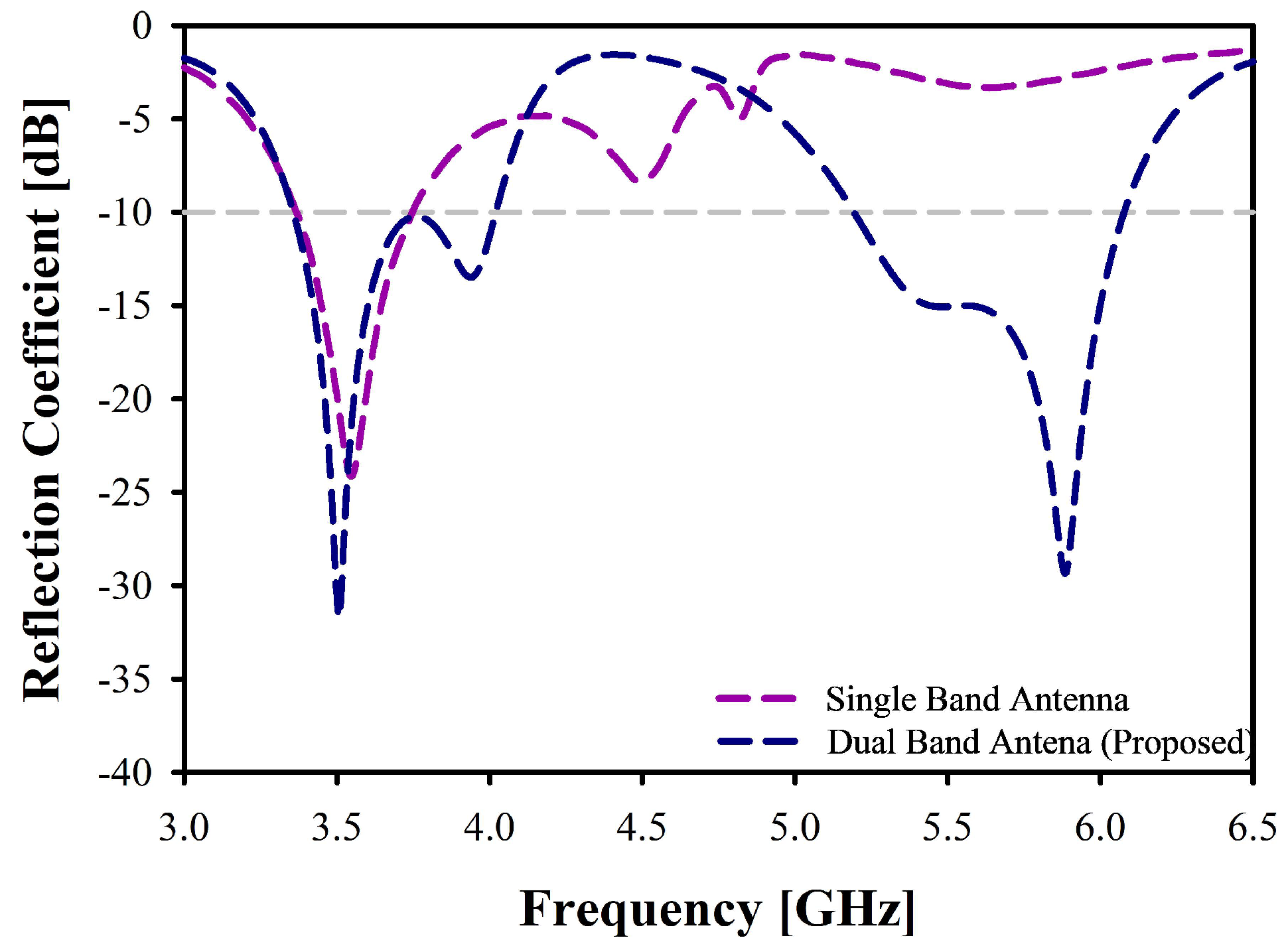
Figure 5.
Realized Gain of the Single-Band Antenna and the Proposed Dual-Band Antenna.
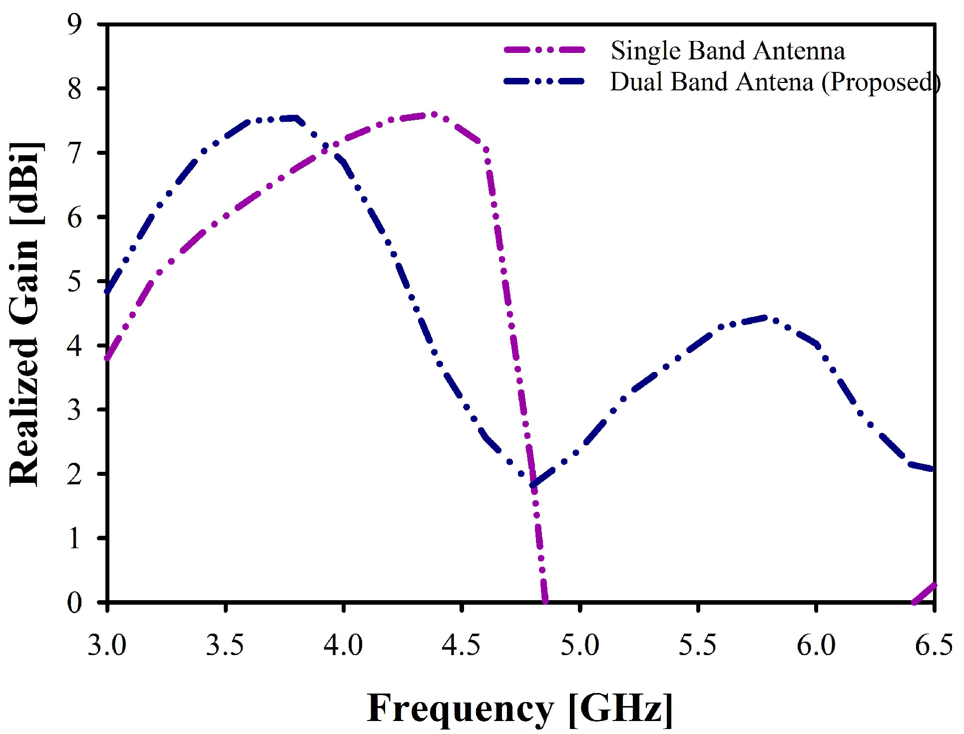
Figure 6.
Methodology for Optimization of Geometric Parameters of the Proposed antenna.
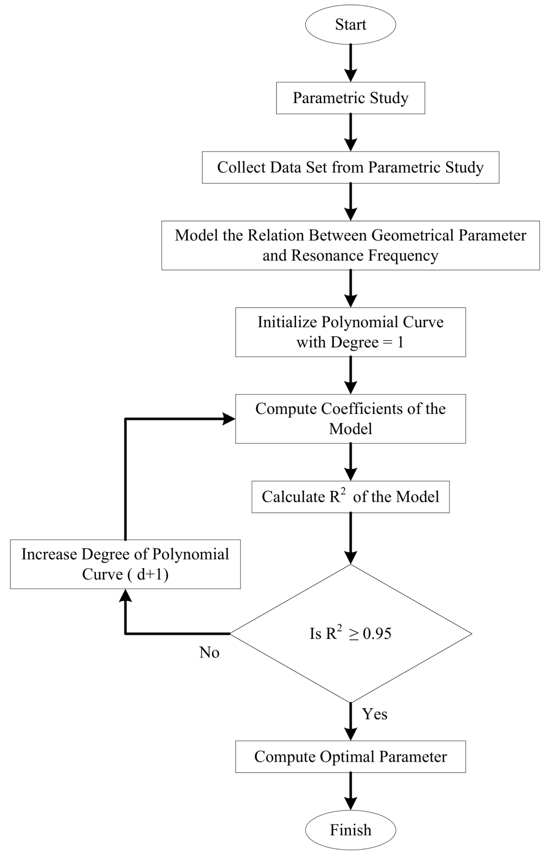
Figure 7.
Reflection coefficient of the antenna for varying parameter D1_L.
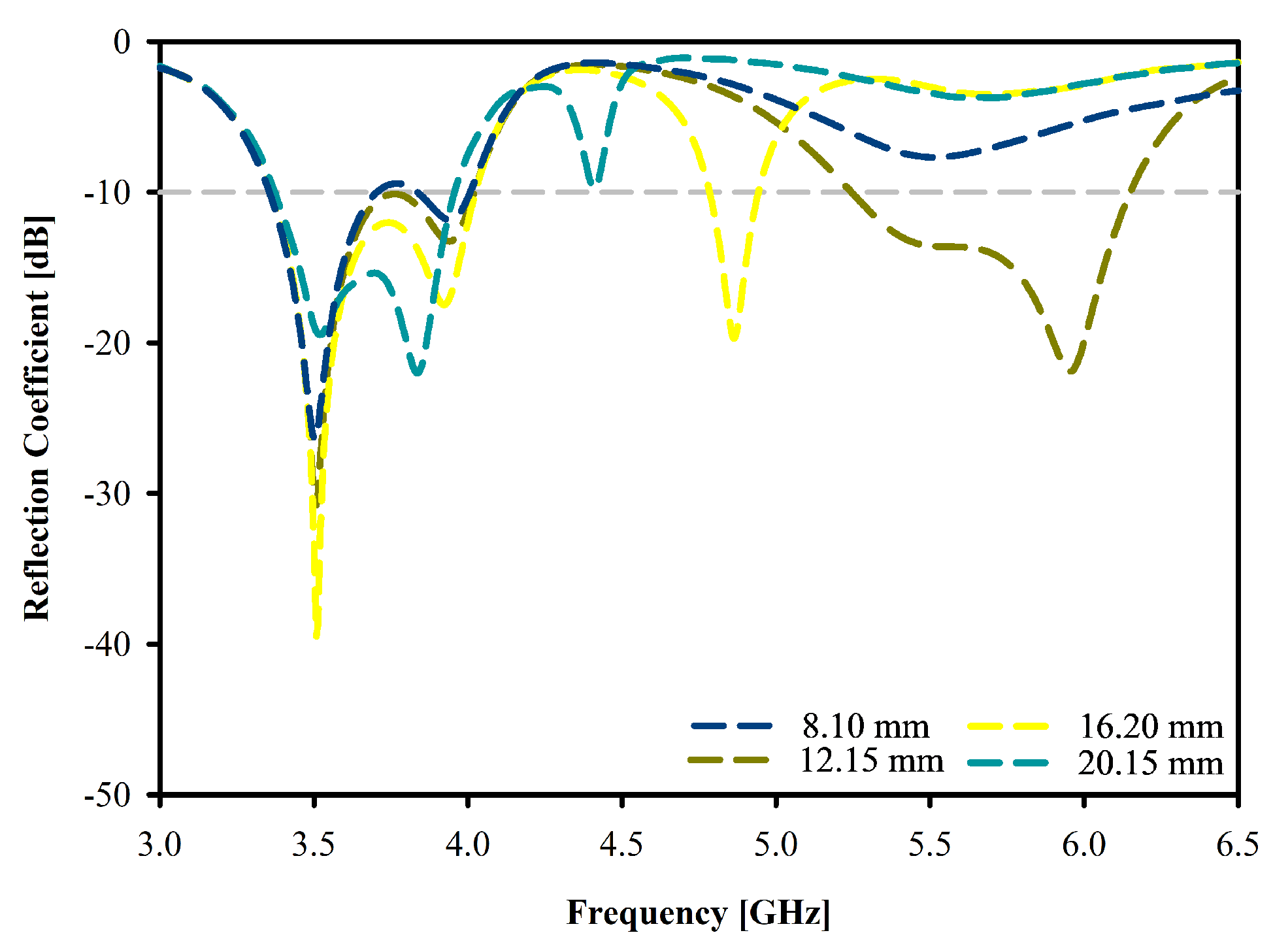
Figure 8.
Reflection coefficient of the antenna for varying parameter D1_S.
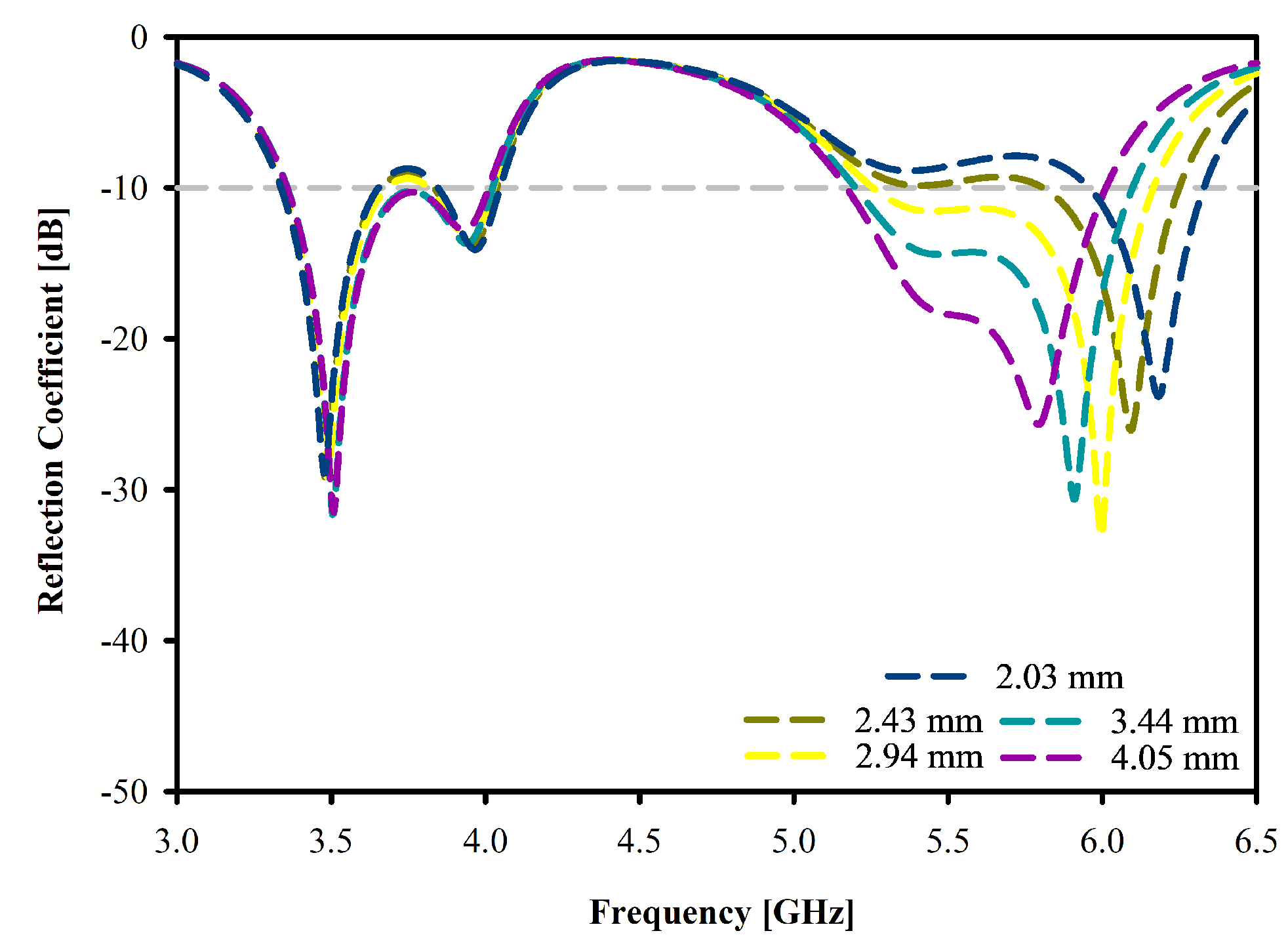
Figure 9.
Reflection coefficient of the antenna for varying parameter D2_L.
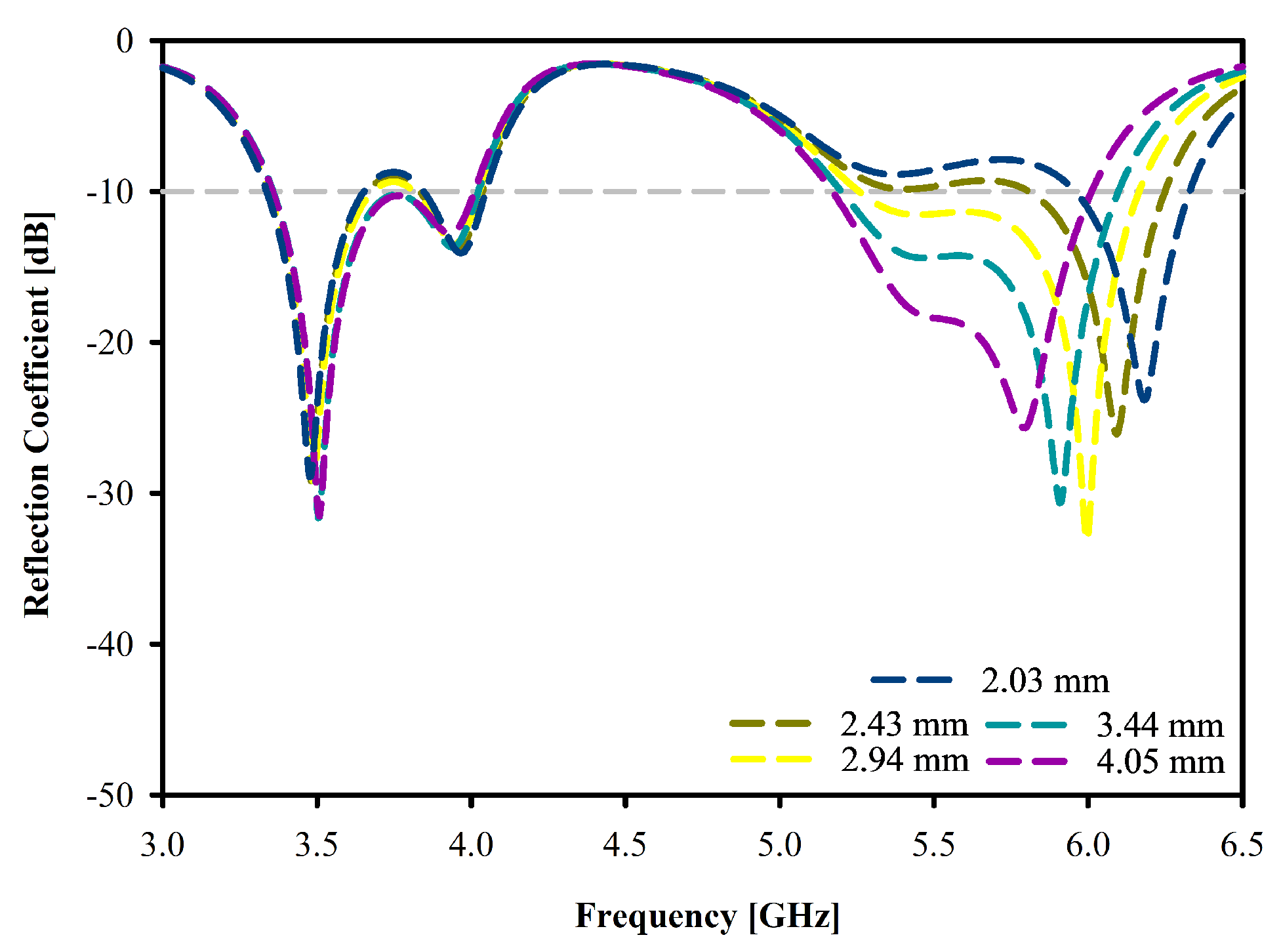
Figure 10.
Reflection coefficient of the antenna for varying parameter D2_S.
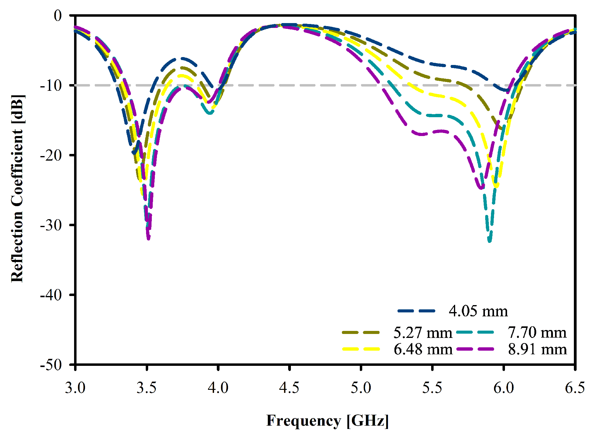
Figure 11.
Reflection coefficient of the antenna for varying parameter D3_L.
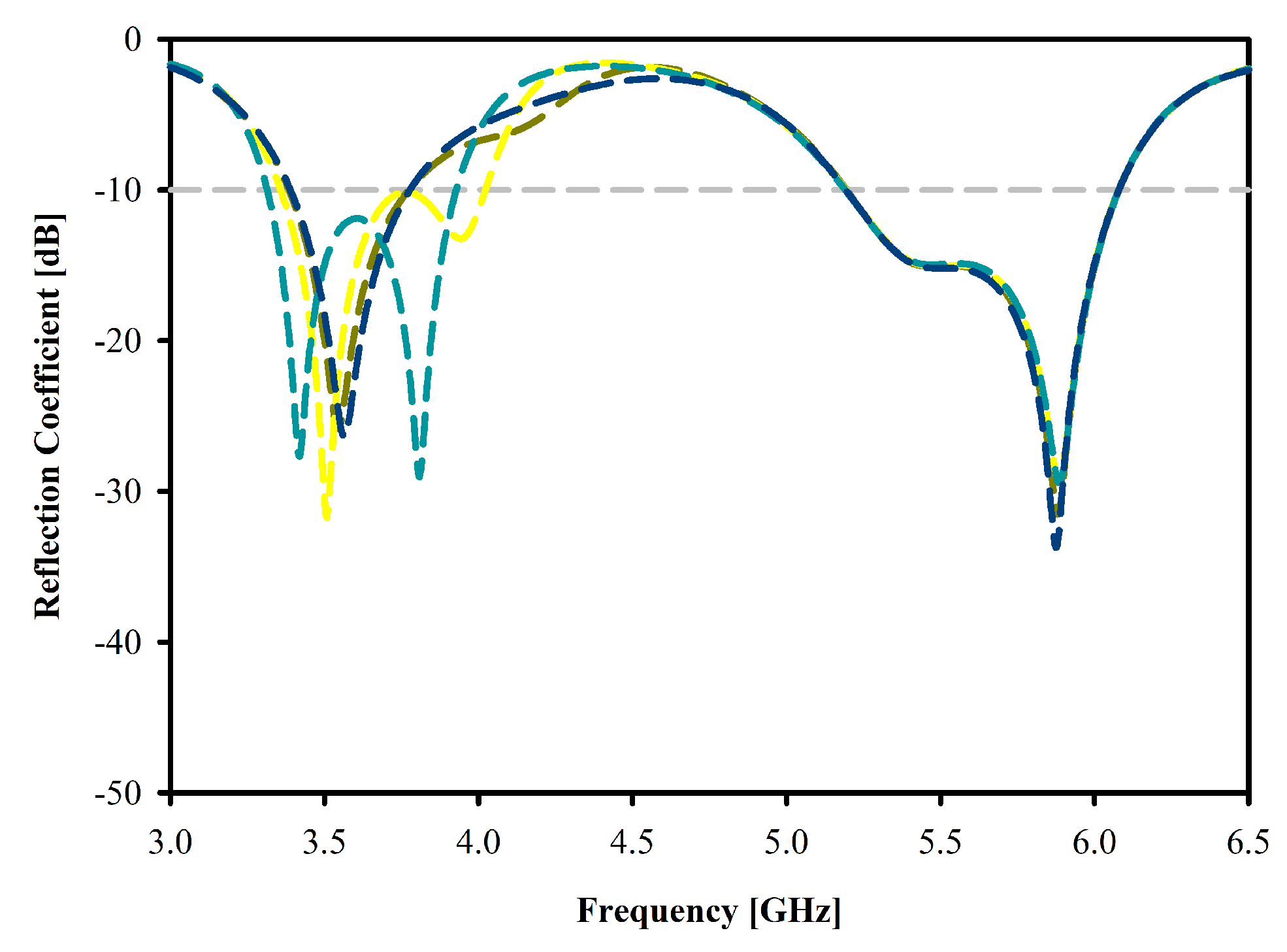
Figure 12.
Reflection coefficient of the antenna for varying parameter D3_S.
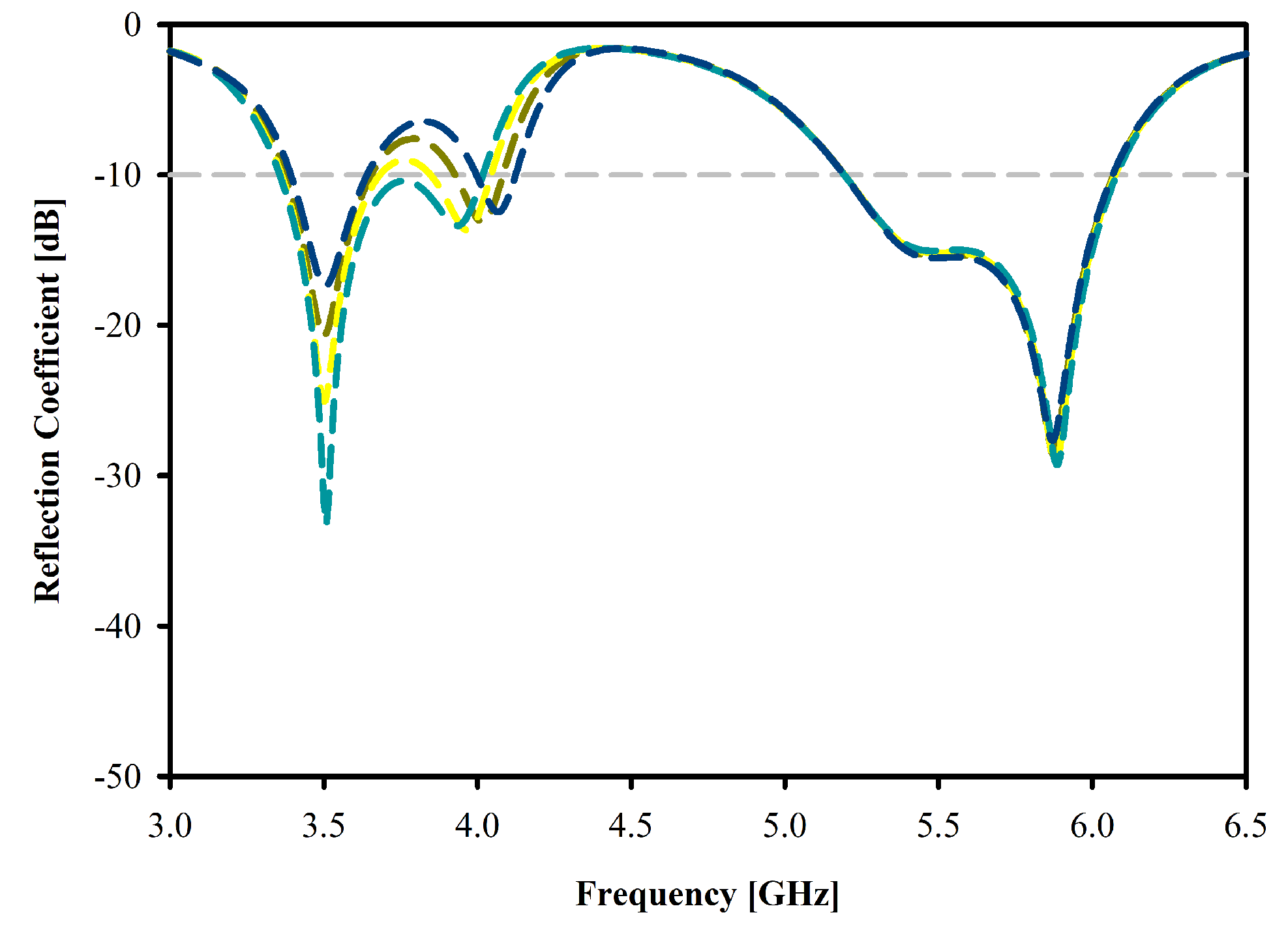
Figure 13.
Fitted Polynomial Curve of the Antenna’s Resonance Frequencies for D1_L Data Points.
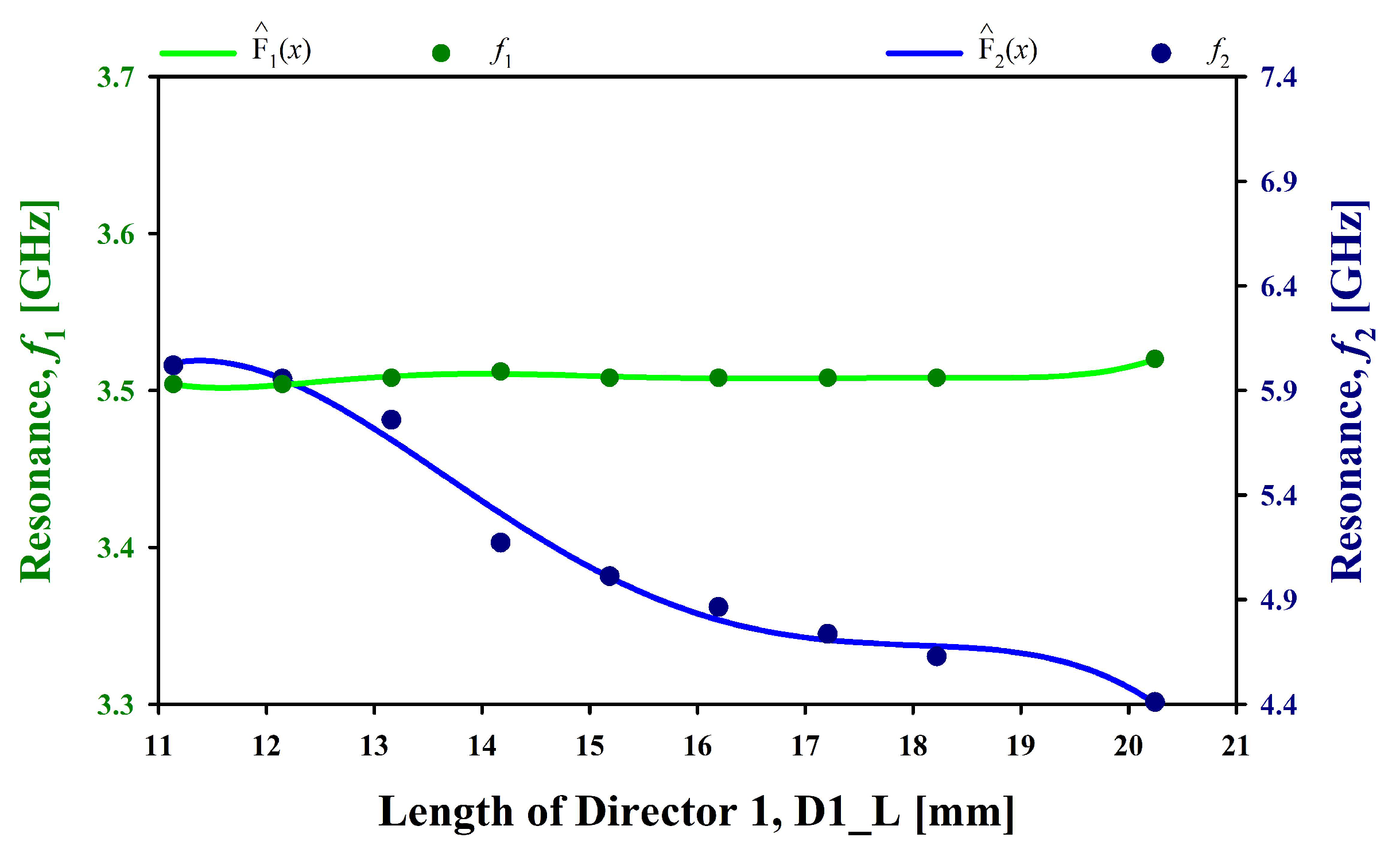
Figure 14.
Fitted Polynomial Curve of the Antenna’s Resonance Frequencies for D1_S Data Points.
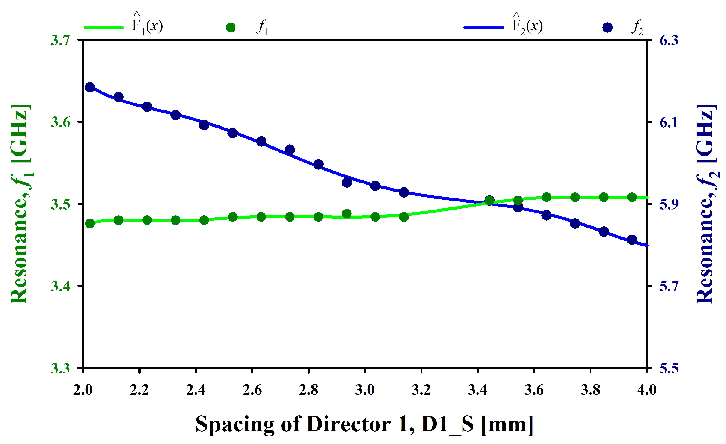
Figure 15.
Fitted Polynomial Curve of the Antenna’s Resonance Frequencies for D2_L Data Points.
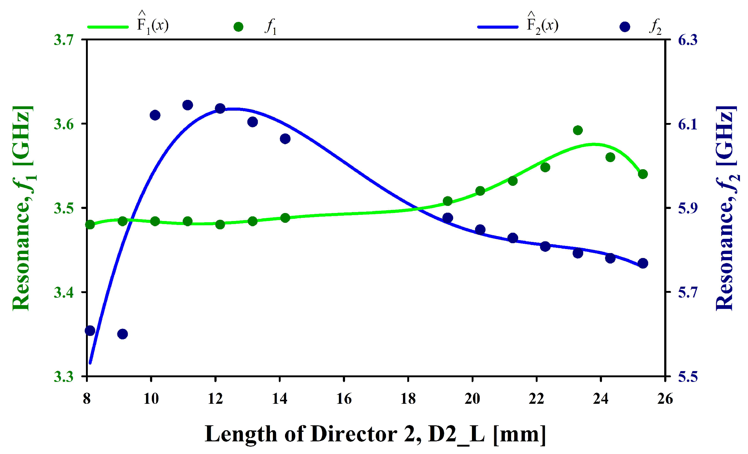
Figure 16.
Fitted Polynomial Curve of the Antenna’s Resonance Frequencies for D2_S Data Points.
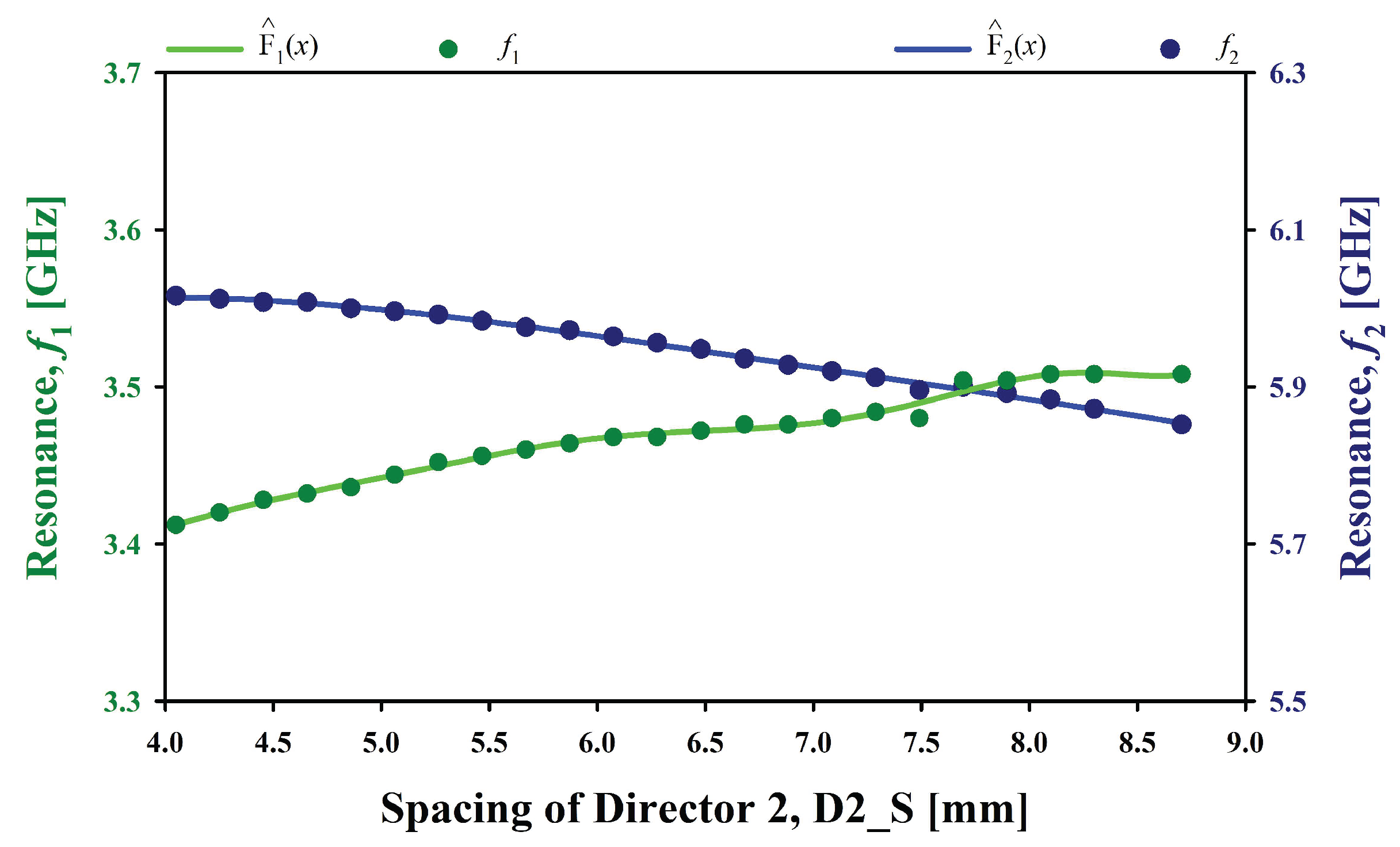
Figure 17.
Fitted Polynomial Curve of the Antenna’s Resonance Frequencies for D3_L Data Points.
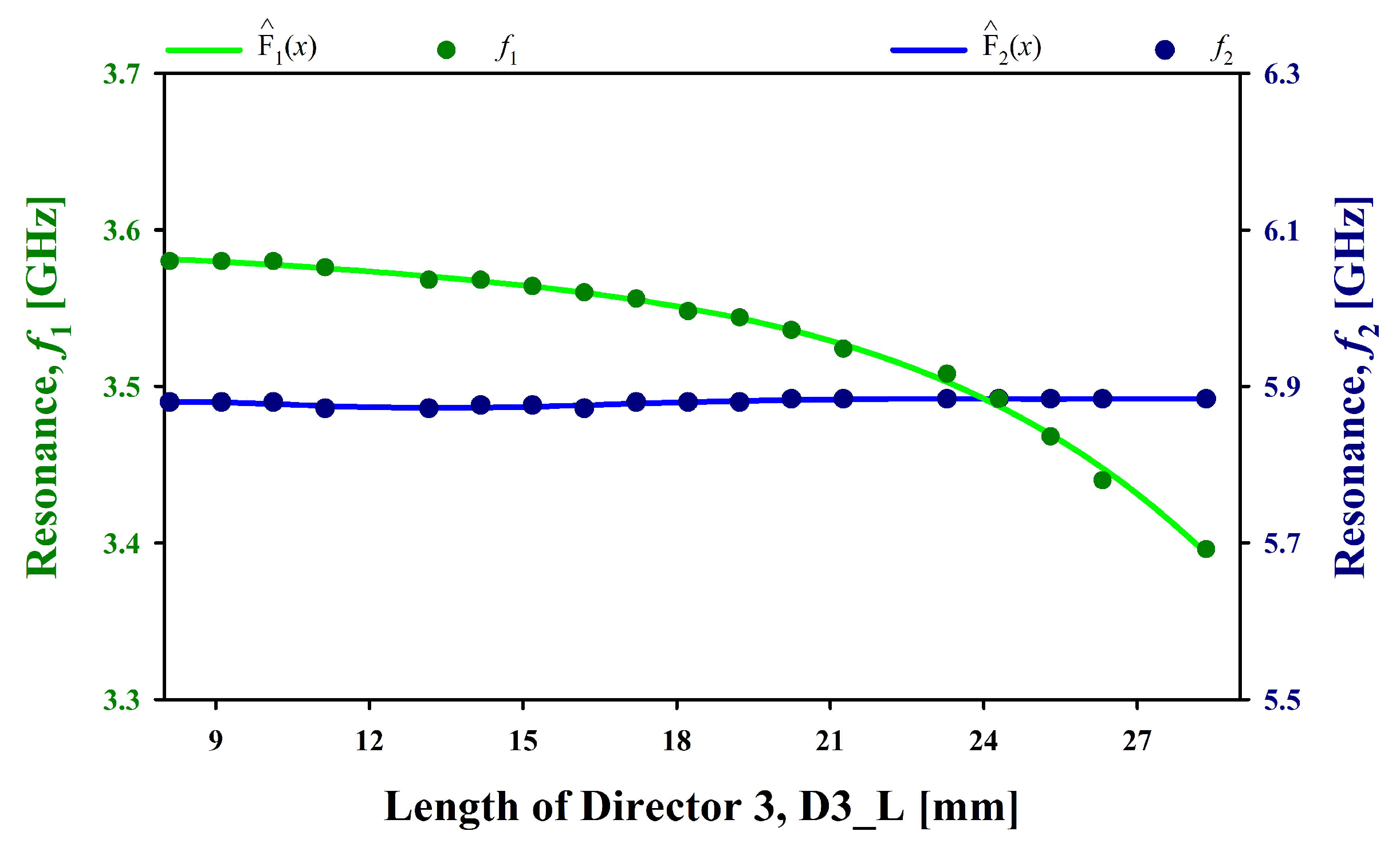
Figure 18.
Fitted Polynomial Curve of the Antenna’s Resonance Frequencies for D3_S Data Points.
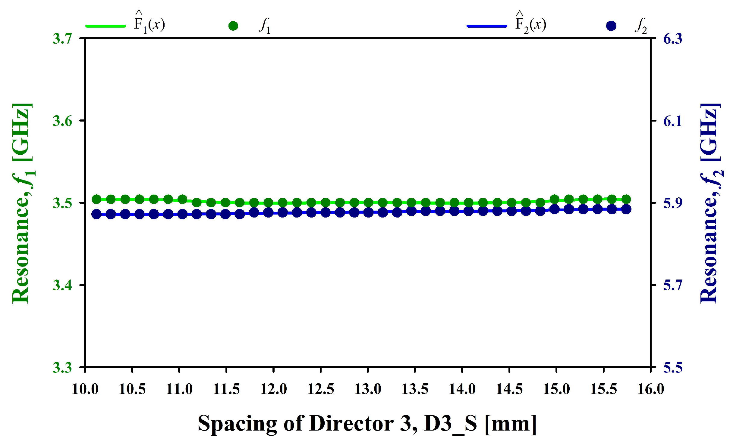
Figure 19.
Current Distribution of the Antenna at Different Frequencies. (a) 3.5 GHz. (b) 5.9 GHz.
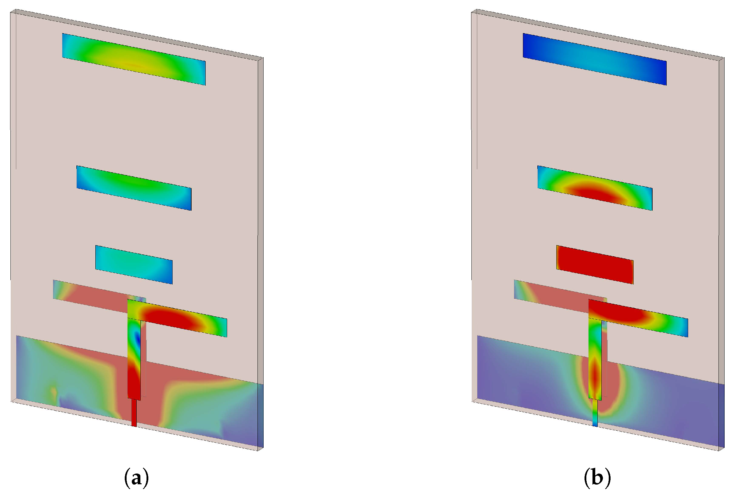
Figure 20.
Prototyped Proposed Antenna and the Measurement Setup. (a) Prototyped Antenna. (b) Measurement Setup.
Figure 20.
Prototyped Proposed Antenna and the Measurement Setup. (a) Prototyped Antenna. (b) Measurement Setup.

Figure 21.
Reflection coefficient of the Proposed Antenna.
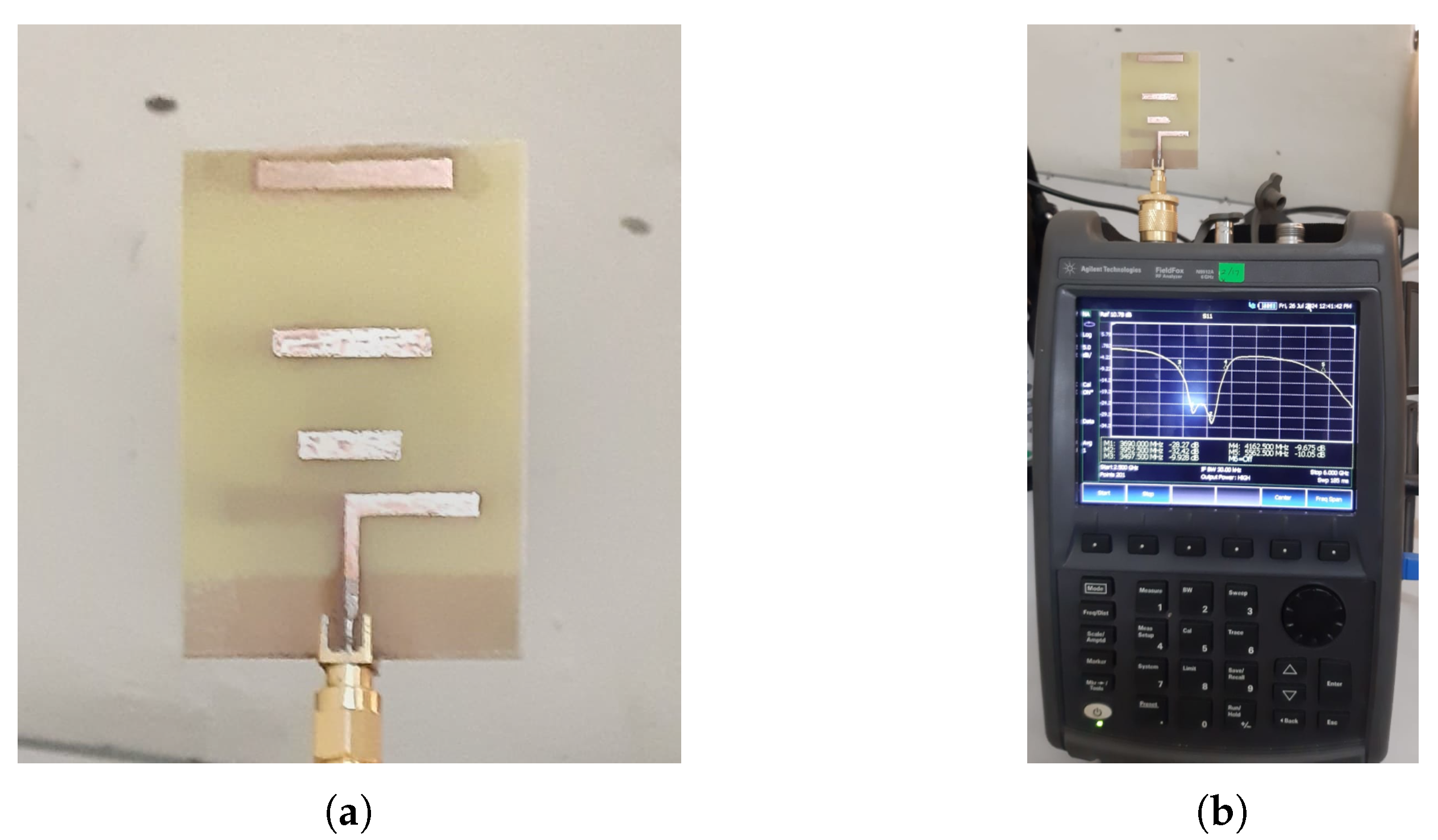
Figure 22.
Gain and Efficiency of the Proposed Antenna.
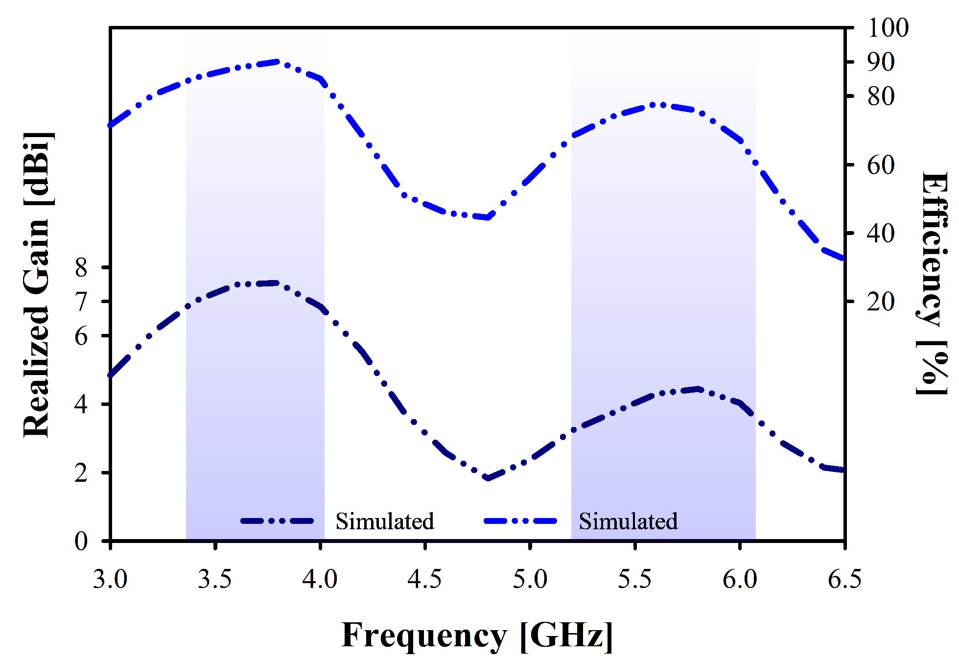
Figure 23.
Normalized Radiation Pattern of the Proposed Antenna. (a) 3.5 GHz. (b) 5.9 GHz.
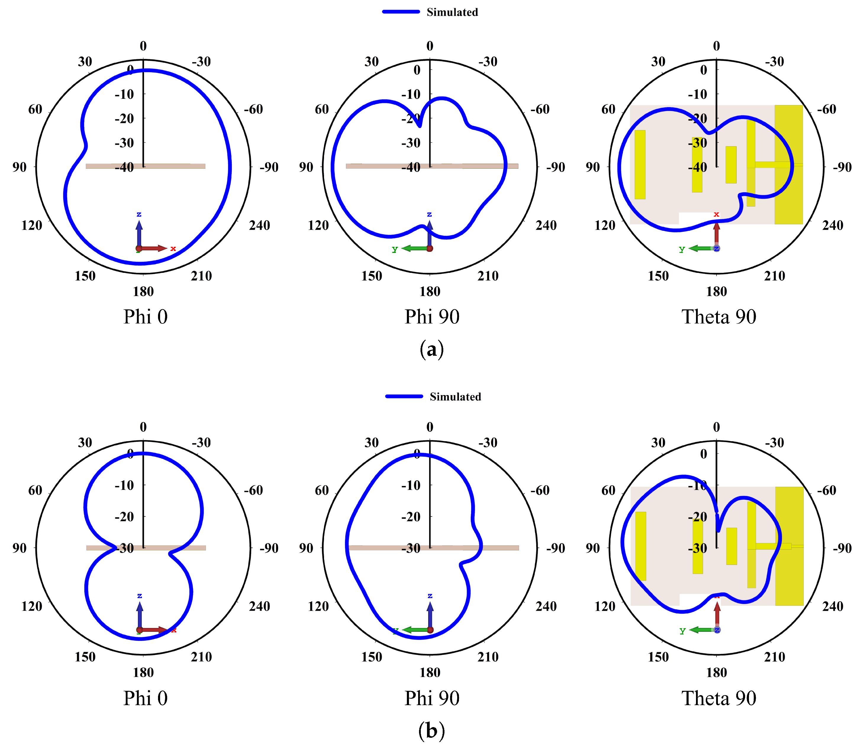
Figure 24.
Proposed Antenna Installed on the Dashboard of a Model Mini Cooper.
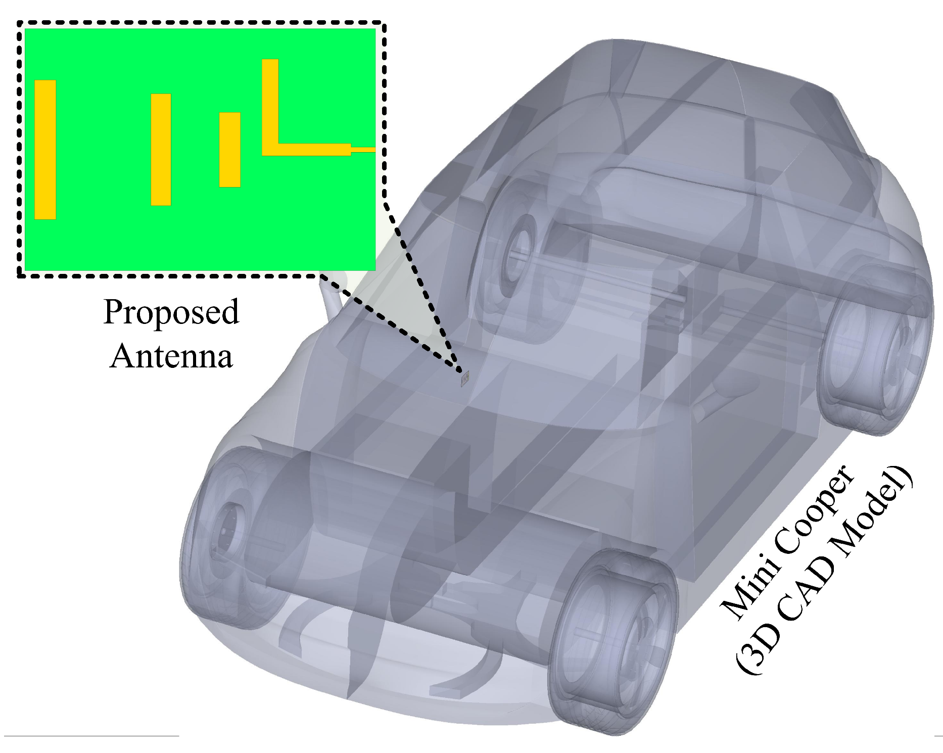
Figure 25.
3D Radiation Pattern of the Proposed Antenna while installed on a car dashboard. (a) 3.5 GHz. (b) 5.9 GHz.
Figure 25.
3D Radiation Pattern of the Proposed Antenna while installed on a car dashboard. (a) 3.5 GHz. (b) 5.9 GHz.
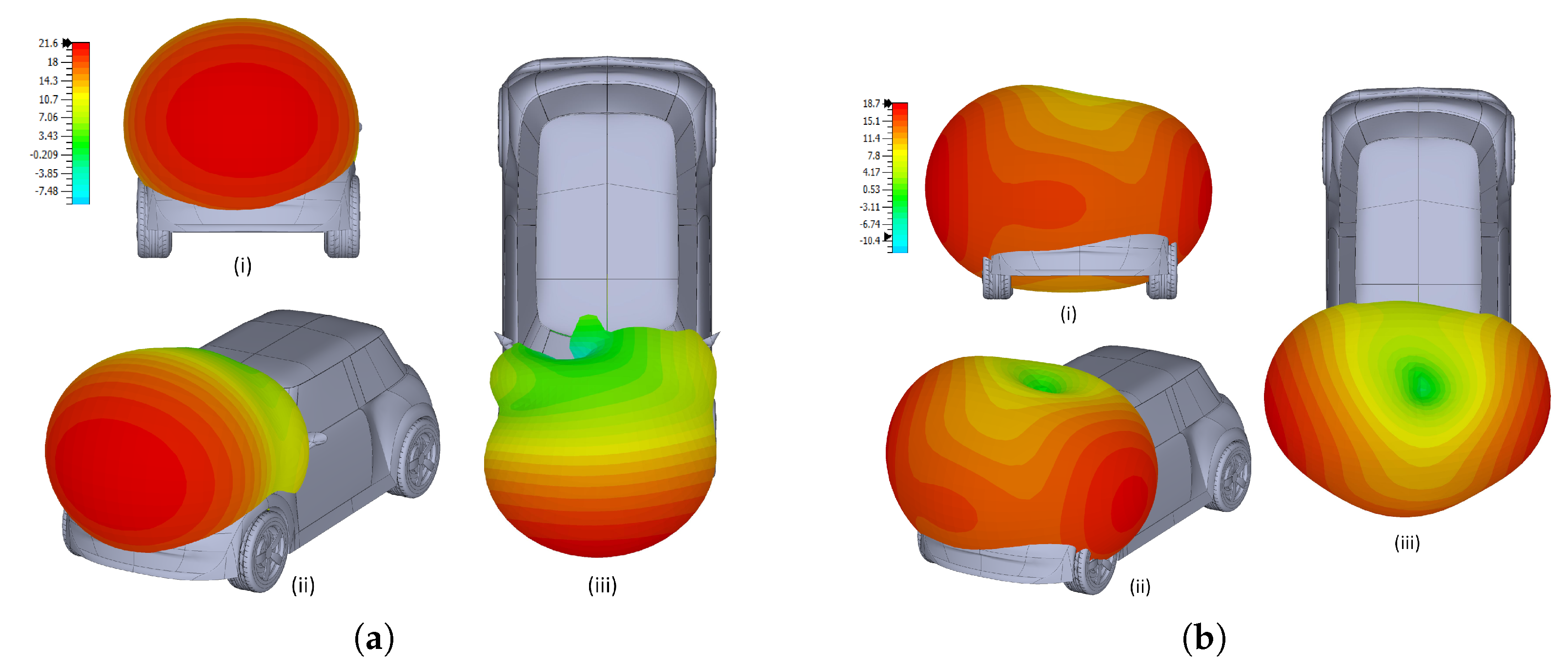
Figure 26.
RLC Equivalent Circuit Model of the Proposed Antenna.
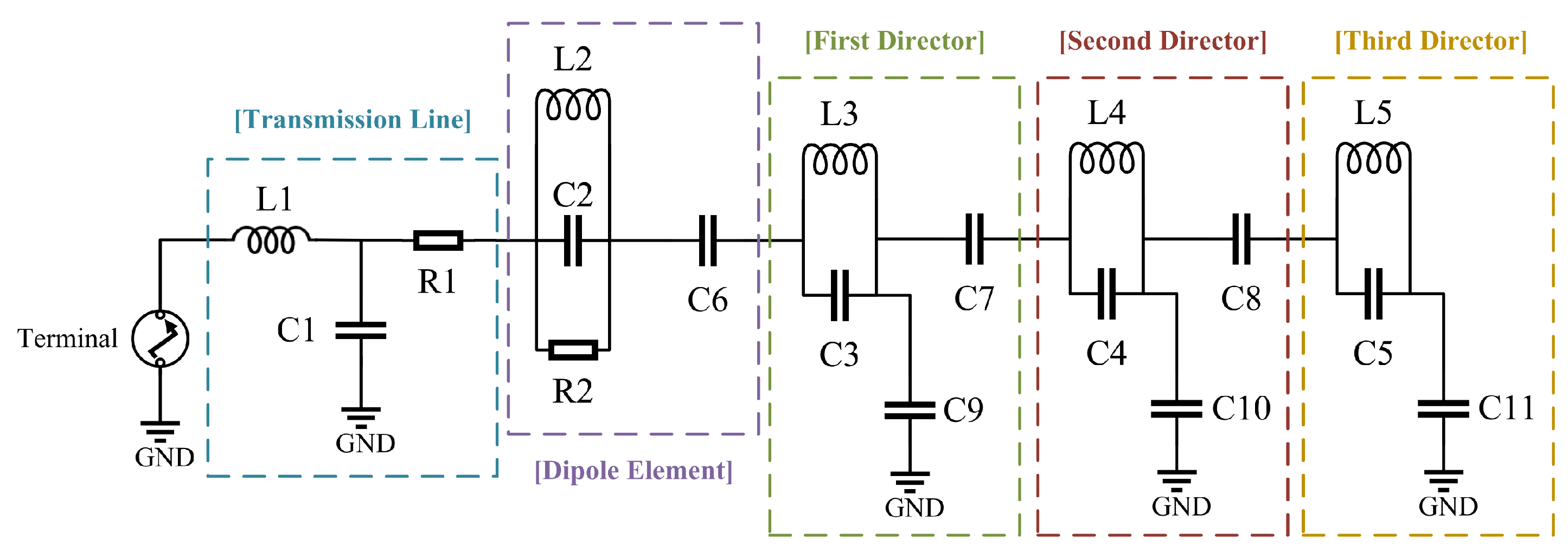
Figure 27.
Reflection Coefficient of the RLC Equivalent Circuit Model.
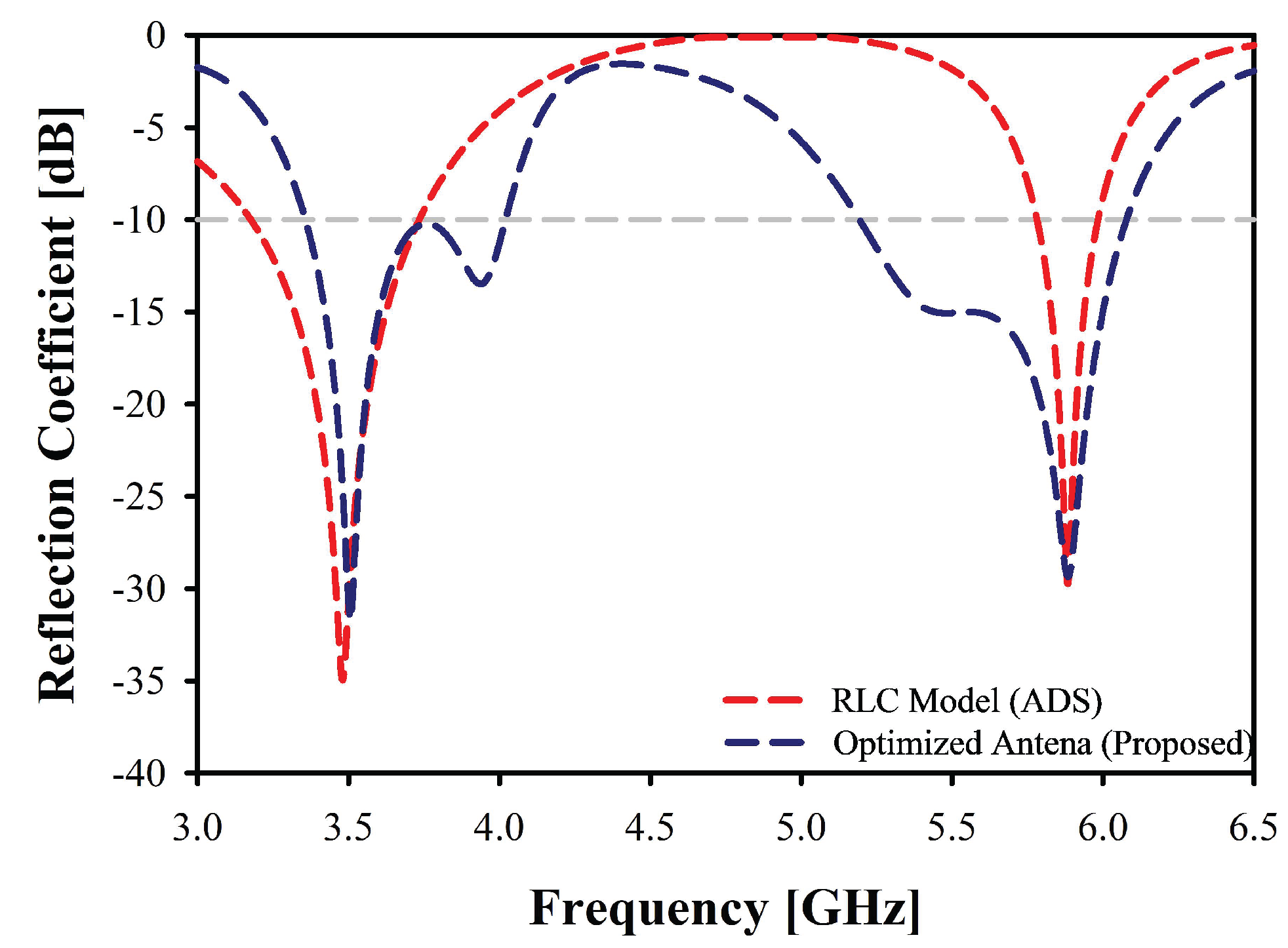

Table 1.
Collected Data Set for Curve Fitting through Parametric Analysis of the Studied Antenna
| Parameter | (MHz) | (MHz) | |
|---|---|---|---|
| Director 1 | D1_L | 3504 — 3520 | 4410 — 6020 |
| 11 mm — 21 mm | |||
| D1_S | 3476 — 3508 | 5792 — 6184 | |
| 2 mm — 4 mm | |||
| Director 2 | D2_L | 3480 — 3592 | 5600 — 6144 |
| 8 mm — 26 mm | |||
| D2_S | 3412 — 3512 | 5820 — 6016 | |
| 4 mm — 9 mm | |||
| Director 3 | D3_L | 3396 — 3580 | 5872 — 5884 |
| 8 mm — 29 mm | |||
| D3_S | 3500 — 3508 | 5872 — 5884 | |
| 10 mm — 16 mm | |||
Table 2.
Performance Comparison of the Proposed Antenna with Recent State of the Art Studies
| Ref | Frequency (GHz) | Bandwidth (GHz) | Efficiency (%) | Peak Gain (dBi) | Size () |
|---|---|---|---|---|---|
| [49] | 3.5, 5.9 | 3.23 - 6.26 | 92 | 5.9 | 0.9×0.35 |
| [47] | 5.9 | 0.4 | 94 | 7.68 | 1.46×1.46 |
| [48] | 5,6 | 4.77 - 6.31 | 93.2 | 4.2 | 3.93×2.95 |
| This Study | 3.5, 5.9 | 0.7, 0.9 | 90.1, 78.4 | 7.55, 4.45 | 0.44×0.64 |
Disclaimer/Publisher’s Note: The statements, opinions and data contained in all publications are solely those of the individual author(s) and contributor(s) and not of MDPI and/or the editor(s). MDPI and/or the editor(s) disclaim responsibility for any injury to people or property resulting from any ideas, methods, instructions or products referred to in the content. |
© 2025 by the authors. Licensee MDPI, Basel, Switzerland. This article is an open access article distributed under the terms and conditions of the Creative Commons Attribution (CC BY) license (http://creativecommons.org/licenses/by/4.0/).
Copyright: This open access article is published under a Creative Commons CC BY 4.0 license, which permit the free download, distribution, and reuse, provided that the author and preprint are cited in any reuse.


