Submitted:
17 November 2025
Posted:
18 November 2025
You are already at the latest version
Abstract
Spatio-temporal planning has emerged as a robust methodology for solving trajectory planning challenges in complex autonomous driving scenarios. By integrating both spatio and temporal variables, this approach facilitates the generation of highly accurate, human-like, and interpretable trajectory decisions. This paper presents a novel model-based spatio-temporal behavior decider, engineered to produce optimal and explainable driving trajectories with enhanced efficiency and passenger comfort. The proposed decider systematically evaluates the action space of the ego vehicle, selecting the trajectory that optimizes overall driving performance. This method is particularly significant for autonomous driving systems, as it ensures the generation of human-like trajectories while maintaining high driving efficiency. The efficacy of the proposed framework has been comprehensively validated through rigorous simulations and real-world experimental trials on a commercial passenger vehicle platform, demonstrating its practical utility and performance advantages.
Keywords:
planning model
; spatio-temporal decider
; behavior planning
; autonomous driving
1. Introduction
Behavior planning is one of the most critical subsystems in an autonomous driving system [1,2]. Benefiting from the advancement of driving models, high-quality and human-like trajectories can now be predicted more naturally. However, driving models do not always predict the correct behavior at the appropriate moment. For safety and other considerations, a robust behavior planning framework is typically expected to help driving models enhance their actual performance [3]. Specifically, driving models should work in conjunction with a proper behavior planner to achieve safe, comfortable, and efficient autonomous driving experiences.
Common behavior planning methods can be categorized into two main types: rule-based planners and model-based end-to-end planners. First, rule-based planners—such as the lattice trajectory planner [4] and Baidu Apollo EM planner [5] are built on heuristic or optimization algorithms. These planners offer strong explainability, ease of maintenance, and computational efficiency, making them widely adopted in several leading autonomous driving systems worldwide. However, their performance may degrade in complex driving scenarios [6]. In contrast, model-based end-to-end planners, do not rely on explicit hand-crafted rules or algorithms [7,8,9,10]. Trained on massive autonomous driving datasets, they excel at solving problems that either require highly complex algorithms or are otherwise computationally intractable. Nevertheless, their training demands enormous volumes of data, and deployed models typically depend on high-performance computing platforms—factors that render their practical and stable application highly challenging [11,12,13].
Building on the unique advantages of the two planner types discussed above, this paper aims to develop a novel algorithm that integrates their respective strengths. The core challenge in our proposed approach lies in the insufficient reliability and stability of trajectories predicted by model-based planners. The underlying reason is that while such planners elevate the upper limit of system performance, they may simultaneously lower the system’s lower bound of operational stability. In contrast, rule-based planners typically make decisions (e.g., lane bias adjustments or lane changes) via predefined algorithms. However, when confronted with complex decision-making scenarios, the cascading effects of these decisions are often not adequately assessed—which may result in hazardous or operationally meaningless outcomes [14]. To address these limitations, this paper proposes a model-based spatio-temporal decider. By evaluating the overall driving performance of trajectories generated by the driving model, the proposed decider ensures the final selected trajectory meets the requirements of safety, comfort, and efficiency. Notably, this spatio-temporal decider has been successfully and rigorously validated through both simulation tests and million-mile real-world experiments across urban and highway scenarios.
The main contributions of this paper are centered on two core modules of the decider: first, it introduces a novel model-based trajectory generation framework tailored to autonomous driving scenarios; second, it designs a dedicated trajectory evaluation algorithm to ensure the effectiveness and robustness of the decider’s output.
The remainder of this paper is structured as follows. Section 2 presents the necessary preliminaries for the subsequent analysis. Section 3 details the main framework of the proposed model-based spatiotemporal decider, with key design principles and component interactions elaborated. Section 4 presents and analyzes the results of both simulations and real-world experiments, including quantitative metrics and qualitative performance insights. Section 5 provides concluding remarks on the study’s contributions and outlines key directions for future work.
2. Preliminaries
In this section, we introduce several key concepts that serve as sub-modules within the proposed model-based spatio-temporal decider. Specifically, the vehicle kinematic model provides the foundational framework for the trajectory planning model, while quadratic programming acts as the core algorithm for smoothing the trajectories generated by the model.
2.1. Vehicle Kinematic Model
In this paper, the bicycle model (as shown in Figure 1) is selected as the vehicle kinematic model, as it effectively balances computational efficiency and modeling accuracy for autonomous driving trajectory planning scenarios [15]. The states of the model are denoted as , where x and y denote the Cartesian coordinates of the rear axle center, denotes the vehicle’s heading, and denotes the steering angle. We define as the inputs, where v is the velocity and is the steering rate. The vehicle kinematic model is shown below.
where is the rotation rate, represents the turning radius. L is the wheelbase. By integrating the formulas above, the state change matrix is finally derived as:
2.2. Quadratic Programming
Quadratic Programming (QP) is a highly efficient optimization method. In this study, QP is employed for trajectory smoothing within a convex space constructed based on a Station-Time (S-T) coordinate system. This optimization approach bears similarities to that adopted in Baidu Apollo’s EM Planner [5]. The fundamental principles of leveraging QP for the aforementioned task are elaborated in this subsection.
The QP problem with speed variables and constraints is formulated in equation (3).
where s is the vehicle position in Frenet coordination, v is the speed, a is the acceleration, and j is the jerk. are the corresponding weights. i is the planning step, and n is the total number of steps during the whole planning horizon. and are the reference position and reference speed respectively.
3. Model-Based Spatio-Temporal Decider
The two core modules of the model-based spatio-temporal behavior decider are elaborated in the subsequent two subsections. Prior to delving into these details, the overall framework of the Model-based Spatiotemporal Decider is first presented. As illustrated in Figure 2, the proposed model-based spatiotemporal decider is embedded within a two-stage end-to-end autonomous driving model architecture. Specifically, the first-stage perception and prediction model takes camera images as input and outputs object detection results and motion predictions. In the planning module, the planning model accepts all static and dynamic perceptual outputs as inputs and then generates multiple candidate trajectories. Based on these candidate trajectories, the spatio-temporal decider makes an optimal selection; the chosen trajectory is subsequently smoothed to meet the control system requirements.
3.1. Trajectory Planning Model
Our trajectory planning model consists of two main networks, a scene encoder process environmental and dynamic information, while a decoder deal with cross-attention to scene encodings and ego motion tokens. The general planner is designed on a transformer architecture. The model size is 0.1 billion. The scene encoder and trajectory decoder will be introduced in the following two subsections.
3.1.1. Scene Encoder
As illustrated in Figure 3, the scene encoder processes diverse inputs and multi-modal data, encompassing the ego-vehicle’s current state, historical states, dynamic traffic agents’ states, road graph, traffic lights, and navigation information. The states of the ego-vehicle and traffic agents are characterized by their positions, velocities, accelerations, and dimensions. Specifically, the ego-vehicle’s current state and dynamic traffic agents’ states are detected from the current frame, while its historical states are aggregated across preceding frames. The integration of the ego-vehicle’s historical information is intended to enhance the planner’s temporal modeling capacity, thereby enabling the generation of continuous and stable trajectories. The road graph includes road boundaries, lane boundaries, stop lines, and other traffic markings. Navigation information comprises general routing details and recommendations provided by the navigation service. After encoding all input data, they are fused into an integrated feature vector. These fused features are subsequently fed into a self-attention block to model intrinsic relationships across the scene. Finally, the scene encoder yields a scene-level fused feature of relatively high dimension.
3.1.2. Trajectory Decoder
As illustrated in Figure 3, the trajectory decoder comprises two main components: one generates a main trajectory, and the other generates auxiliary trajectories. Details of these two decoder heads are elaborated below.
The main trajectory is decoded via a Transformer decoder architecture, where the query is primarily derived from the ego-vehicle’s position embedding, and the keys and values are the fused scene features output by the scene encoder. The ego-vehicle’s position embedding and scene features are processed through cross-attention to model internal relationships. The trajectory features, output by the main trajectory cross-attention module, are then converted into final main trajectory points via a multi-layer perceptron (MLP). The Transformer decoder is configured with a dimension of 256 and 8 layers. The main trajectory consists of 24 points, forming a 6-second trajectory with a time resolution of 0.25 seconds. Corresponding to the main trajectory decoder, two loss functions are designed: an imitation loss and a collision loss. The imitation loss aims to guide the model to mimic human driving trajectories using ground truth data. To further ensure safety, the collision loss is calculated based on the distance between the ego-vehicle’s trajectory bounding box and the bounding boxes of agents’ trajectories in the ground truth. These two losses are summed to form the total loss, with the imitation loss assigned a dominant weight.
To enhance trajectory diversity, an auxiliary trajectory decoder head is also designed. For this purpose, the ego-vehicle’s position embedding is merged with predefined trajectory anchors to form the query for the Transformer. These trajectory anchors are determined based on statistical analysis of the diversity in ground truth trajectories. Specifically, 48 anchors are defined to meet diversity requirements, covering lane changes, turns, U-turns, and other typical maneuvers. Similar to the main trajectory decoder, the keys and values here also use the fused scene features from the scene encoder, and the Transformer decoder shares the same configuration (256 dimension, 8 layers). For each anchor in the fused query, a corresponding trajectory is encoded in the auxiliary trajectory feature. This feature is first mapped to auxiliary trajectories through an MLP structure. Unlike the main trajectory, this head outputs 48 trajectories, each consisting of 24 points to form a 6-second trajectory (with a 0.25-second resolution). Additionally, the probability of each auxiliary trajectory is critical within the overall spatio-temporal framework, as it provides a ranking mechanism. The probability of each auxiliary trajectory is determined by its similarity to the ground truth trajectory.
3.1.3. Training Dataset
The training dataset for the planning model comprises 5 million video clips, each 20 seconds in duration. Each clip is split into 20 pickle files, with each file containing 10 seconds of historical data and 20 seconds of future data. Altogether, this results in a total of 100 million pickle files across the entire dataset. All data are collected via a customer-owned vehicle fleet, which contributes over 1 million new clips monthly—supporting ongoing model iteration and expansion. As illustrated in Figure 4, a sample pickle file encapsulates all essential information, including road graphs, as well as ground truth trajectories of the ego-vehicle and surrounding agents. The dataset covers a diverse range of scenarios, with distributions as follows: urban roads (80%), city expressways (10%), and highways (10%). Within the urban road category specifically, typical driving scenarios and maneuvers are comprehensively included, such as intersections, U-turns, straight driving, lane changes, and other common operations.
3.2. Spatio-Temporal Evaluation
As outlined in Section 3.1, the planning model generates one main trajectory and 48 auxiliary trajectories. Herein, we evaluate all generated trajectories and select the optimal one as the final executable trajectory. The core of the trajectory evaluation module lies in the formulation of evaluation criteria. Given that the quality of the model’s output trajectories has already been validated by the training metrics—with guaranteed high performance and safety—we adopt a simplified heuristic evaluation framework, focusing on three key dimensions: travel efficiency, riding comfort, and lateral stability. Detailed evaluation methodologies are elaborated below.
3.2.1. Efficiency Cost
Travel efficiency of a trajectory is evaluated based on two core metrics: terminal speed and total trajectory length. As the planning horizon of the model is set to 6 seconds, the vehicle’s terminal speed (at the 6-second mark) directly reflects efficiency—with higher terminal speed indicating superior efficiency. Beyond terminal speed, the total trajectory length (i.e., the distance traveled by the vehicle within the 6-second planning window) is also considered, where a longer trajectory corresponds to higher efficiency. To standardize the evaluation scale, the costs associated with terminal speed and trajectory length are normalized relative to a “do-nothing trajectory” (a baseline trajectory with no active maneuvering), which is achieved by calculating a speed loss and a length loss respectively. The speed loss is calculated as
The length loss is calculated as
Each loss contributes 50% to the total efficiency cost, which is a number between 0 to 1. The efficiency cost is calculated as
3.2.2. Riding Comfort Cost
Riding comfort of a trajectory is evaluated based on two key metrics: the maximum absolute longitudinal acceleration and the maximum absolute centripetal acceleration (lateral acceleration equivalent). The riding comfort cost increases with the magnitude of either metric—higher maximum values correspond to poorer comfort and thus higher costs. Specifically, the maximum absolute longitudinal acceleration is defined as the absolute value of the maximum or minimum longitudinal acceleration across the entire trajectory. The maximum absolute centripetal acceleration refers to the absolute value of the maximum or minimum centripetal acceleration along the trajectory, which directly reflects lateral comfort performance. For each trajectory point, the centripetal acceleration is calculated as , where v denotes the speed at the target trajectory point and represents the curvature of the corresponding path point. Accordingly, the longitudinal and lateral riding comfort costs are computed as follows:
The longitudinal and lateral riding comfort costs each account for 50% of the total riding comfort cost, which is also normalized to a value ranging from 0 to 1. The total riding comfort cost is calculated as follows:
3.2.3. Lateral Stability Cost
The lateral stability of a trajectory is characterized by two metrics: its similarity to the previously planned trajectory and its proximity to the lane centerline. Specifically, for the first metric, the lateral deviation (denoted as ) between the terminal point of the evaluated trajectory and that of the previously planned trajectory is calculated within the same coordinate system. The cost associated with this lateral deviation is computed as follows:
Second, the lateral offset (denoted as ) between the terminal point of the evaluated trajectory and the lane centerline is computed. The cost associated with this lateral offset is calculated as follows:
The lateral deviation cost and lateral offset cost each account for 50% of the total lateral stability cost, which is also normalized to a value ranging from 0 to 1. The total lateral stability cost is calculated as follows:
3.2.4. Total Cost
The total cost is the weighted sum of efficiency, riding comfort, and lateral stability cost.
Since each cost has been individually normalized (to the range [0,1]), we can directly identify the optimal trajectory and assess whether it offers sufficient performance gains relative to the do-nothing trajectory. If the optimal trajectory demonstrates a distinct advantage over the do-nothing trajectory, we execute the corresponding maneuver decision and pass the optimal trajectory to a refined trajectory planning process. Two criteria are used to validate this distinct advantage:
If both of the above two criteria are satisfied, the selected optimal trajectory demonstrates a distinct advantage over the do-nothing trajectory. Accordingly, the vehicle executes the corresponding driving maneuver in accordance with the optimal trajectory (e.g., lane keeping with lateral biasing, lane changes).
3.3. Lightweight Trajectory Smoother
Based on the evaluation results, an optimal trajectory is selected. To enhance the drivability of this trajectory, we design a QP-based lightweight trajectory smoother (see [5]).
First, the feasible solution space for the QP problem is determined. We utilize the vehicle’s kinematic upper and lower bounds to calculate the corresponding bounds of vehicle states at each planning timestamp. Here, the time interval is reduced from 0.25 s to 0.1 s to enhance trajectory smoothness. Within these upper and lower bounds, the optimization reference at each time instant is the original trajectory generated by the planning model. Specifically, the reference values for acceleration and jerk are both set to zero.
At this stage, all necessary elements for formulating the QP problem (as outlined in Section 2.2) are established, whose main objective is to smooth the trajectory’s longitudinal performance. As detailed in Section 2.2, the QP optimizer is subject to several constraints: the minimum speed is set to zero, while the maximum speed is constrained by the allowable speed limit; for acceleration and jerk, the ranges are configured to ensure riding comfort.
The output speed profile from QP optimization yields a 6-second smoothed trajectory characterized by high resolution, superior lateral and longitudinal smoothness, and enhanced flexibility.
4. Simulation and Experiments
We validated the effectiveness of the proposed method through both simulations and physical experiments. Two common urban driving scenarios—dynamic obstacle avoidance within intersections and narrow road driving—were selected for testing. In each scenario, we first validated the proposed algorithm via simulations, followed by subsequent physical experiments to further verify its performance.
4.1. Dynamic Avoidance in Intersection
Intersections—especially unprotected ones—are notoriously challenging scenarios for autonomous driving. The ego-vehicle engages in strong dynamic interactions with other road users while maintaining adequate safety margins, which tests the capability of a driving system primarily in terms of safety and efficiency.
4.1.1. Simulation
Our intersection scenario is simulated in a self-developed autonomous driving simulation platform, incorporating all core functional modules required for autonomous driving—including perception, trajectory prediction, ego-vehicle state estimation, planning, and motion control. The simulation operates at a 12 Hz update rate, which fully satisfies the safety-critical requirements for autonomous driving systems. The architecture of the planning framework within the simulation is consistent with that depicted in Figure 2.
As illustrated in Figure 5, the scenario considers a fully unprotected, unsignalized intersection where agents from all approach directions may enter freely. The ego-vehicle enters the intersection from the south approach and is tasked with executing a left turn; two concurrent agents are introduced to enter the intersection simultaneously: agent A travels straight, while agent B is also assigned a left-turn maneuver. In this configuration, the ego-vehicle engages in dynamic interactions with both agent A and agent B, resulting in potentially divergent driving strategies. For this scenario, the proposed planning model generates one main trajectory involving yielding to both agent A and agent B. Two auxiliary trajectories are also generated: one overtakes agent B with concurrent yielding to agent A, and the other first proceeds straight to yield to both agent A and agent B prior to executing the left turn.
Simulation results are presented in Figure 6. At the initial time step (t=0s), the ego-vehicle and agents A and B enter the same intersection at different speeds. Agent A holds right-of-way and travels at the highest speed. The model’s main trajectory yields to both agents A and B, while the first auxiliary trajectory yields to agent A and overtakes agent B; the second auxiliary trajectory proceeds straight to yield to agent A before overtaking agent B. Through evaluation, the main trajectory exhibits the lowest cost and is thus selected.
At t=1s, Agent A enters the intersection. As agent B is blocked by agent A, the model generates a new main trajectory to overtake agent B, whereas the first auxiliary trajectory continues to yield to agent B.
At t=2s, the ego vehicle and agent B encounter each other within the intersection. Given agent B’s superior positional advantage, the ego vehicle is required to yield to agent B, and all trajectories generated by the model accordingly yield to agent B.
At t=3s, the ego vehicle successfully yields to agent B, begins accelerating, and proceeds to exit the intersection. Throughout the entire process, the main trajectory is consistently selected due to its safety and reasonableness in this complex interaction scenario.
4.1.2. Experiment
The experiment was conducted in an open urban driving environment, with the scenario similar to that of the simulation. The test vehicle is a Xpeng G9 MAX equipped with dual Orin-X SOCs (508 TOPS), two 126-line solid-state lidars, five radars, and twelve ultrasonic sensors. Lane-line detection results, localization data, and sensor fusion outputs are fed to the planning module as inputs. An experimental video is provided in Supplementary Material Video 1.
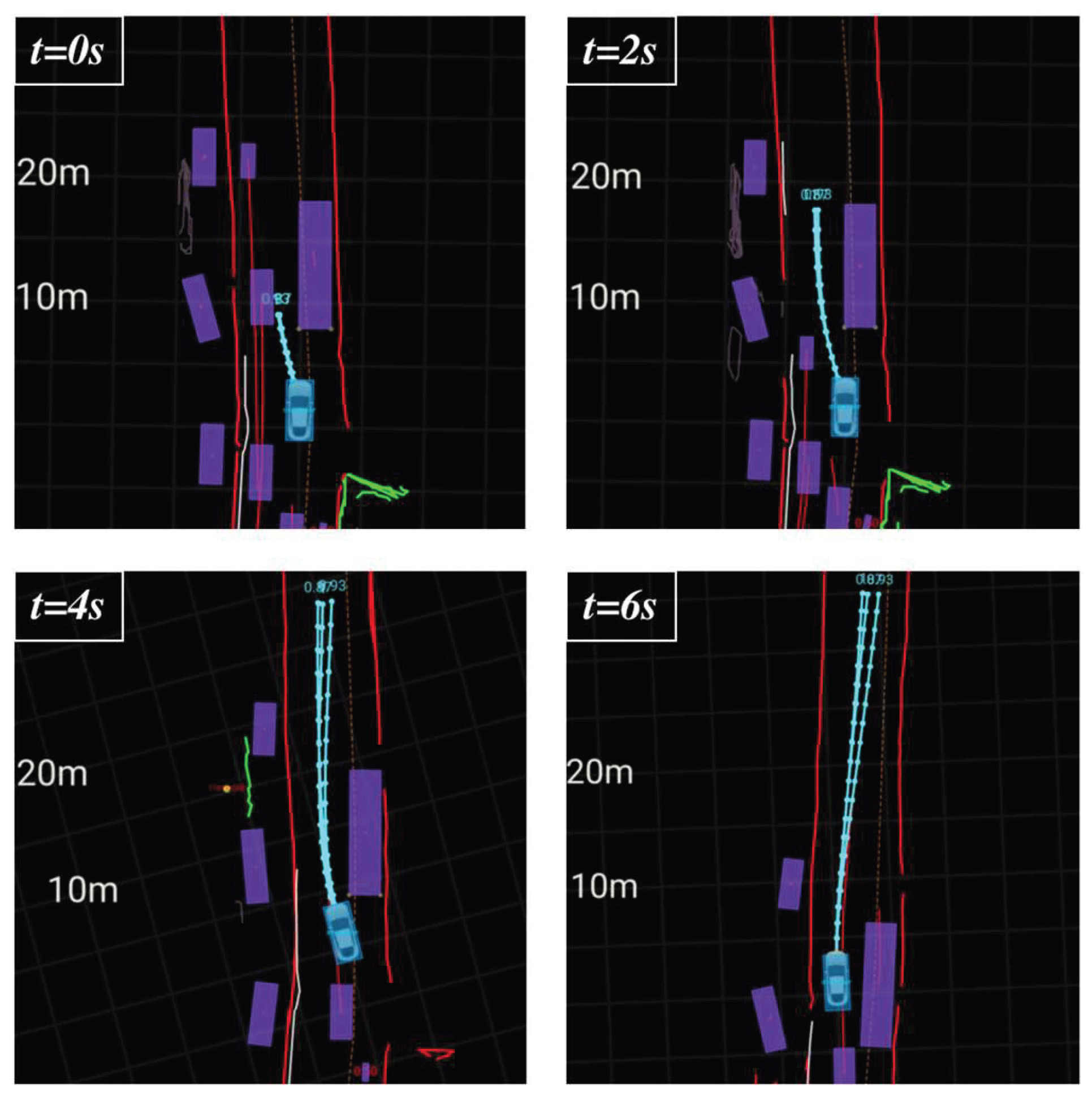
As illustrated in Figure 7, the ego-vehicle enters an unprotected intersection and encounters an oncoming vehicle whose driving direction is initially unknown (assumed to travel straight for initialization). The proposed planning model generates three trajectories (represented by blue lines and trajectory points), all of which yield to the oncoming vehicle. Each trajectory is labeled with its probability at the terminal point. As shown in the figure, the main trajectory’s probability remains consistently 1.0, while the probabilities of the two auxiliary trajectories are less than 1.0.
At t=2s, as the oncoming vehicle executes a left turn, the main trajectory tends to deviate leftward, whereas the two auxiliary trajectories exhibit conflicting maneuver intentions. Following evaluation, our system selects the main trajectory. At t=4s, as the key agent (oncoming vehicle) moves away, the ego-vehicle continuously completes the left turn and then accelerates to exit the intersection. This experiment demonstrates the system’s capability to navigate unprotected intersections under the condition of uncertain intentions of other agents while maintaining reasonable driving efficiency.
4.2. Narrow Road Bypassing
Driving on narrow roads poses significant challenges, as it demands high agility and stable planning capabilities. Slow-moving vehicles and obstructions are the main challenges in narrow road driving scenarios, where bypassing capability is critical. The ego-vehicle must navigate around unpredictable objects while maintaining adequate safety margins; in some cases, it may even need to utilize the opposite lane, which can lead to intense interactions with oncoming vehicles.
4.2.1. Simulation
The narrow road bypass scenario is illustrated in Figure 8. A slow-moving vehicle travels ahead of the ego-vehicle. To bypass this leading slow-moving vehicle(marked as vehicle A), the ego-vehicle needs to utilize the opposite lane and accelerate. As depicted in the figure, the planning model generates multiple trajectories for this scenario: the main trajectory deviates leftward to bypass the leading slow-moving vehicle from the left with adequate safety margins; one auxiliary trajectory performs the same maneuver but maintains a smaller distance from the slow-moving vehicle; the other auxiliary trajectory chooses to follow the slow-moving vehicle while remaining in the original lane.
The simulation results for the narrow-road bypass scenario are illustrated in Figure 9, where the ego-vehicle detects that the preceding vehicle is traveling at a low speed and initiates an overtaking maneuver. At t=0s, the proposed planning model generates three trajectories: one main bypass trajectory, one auxiliary bypass trajectory, and one following trajectory. At this instant, our evaluation system selects the main trajectory, as it achieves the highest efficiency while maintaining adequate safety margins.
After 1 s, with the ego-vehicle’s heading already shifted leftward, all trajectories generated by the model adopt the same bypass maneuver. The evaluation system then selects the safest option, namely the main trajectory. At t=2s, the main trajectory is retained to ensure lateral stability. At t=3s, once the ego-vehicle successfully overtakes vehicle A, the main trajectory—configured to proceed straight—continues to be selected.
4.2.2. Experiment
The experiment was conducted on an open urban narrow road with a single lane in each direction. As illustrated in Figure 10, the ego-vehicle detected a bus stopped with its emergency lights activated ahead; the proposed model’s default response was to utilize the left opposite lane to bypass the bus. At t=0s, the main and auxiliary trajectories exhibited consistent maneuver intentions. However, the left opposite lane was occupied by oncoming vehicles, so all generated trajectories maintained a low speed to ensure safety.
At t=2s, as the oncoming vehicles gradually passed, the trajectories generated by the model began to accelerate. At t=4s, with the opposite lane fully clear for travel, the trajectories continued to accelerate. At t=8s, the ego-vehicle successfully bypassed the stopped bus and slowly merged back into its original lane.
Throughout the entire process, since the main and auxiliary trajectories demonstrated nearly identical efficiency, the spatio-temporal evaluation focused primarily on lateral stability between frames—ultimately favoring the selection of the main trajectory. This result verifies that the main trajectory generated by the proposed model performs effectively in this scenario. The experimental video is provided in Supplementary Material Video 2.
5. Conclusions
In this paper, a model-based spatio-temporal decider is proposed. To generate multi-modal trajectories, a dedicated planning model is designed, with details of its architectural design and training dataset presented herein. Subsequently, a spatio-temporal evaluation framework is developed to select the optimal trajectory from the candidate trajectories output by the planning model.
This work demonstrates exceptional practical efficiency, as it integrates the high performance advantages of data-driven approaches while ensuring stable operational performance through the proposed spatio-temporal evaluation mechanism. The significance of the proposed method lies in two key aspects: theoretically, the model-based framework exhibits strong extensibility, allowing for multiple structural modifications to support diverse decision-making tasks or combined decision strategies in complex driving environments. Practically, the method can be seamlessly deployed on most autonomous driving platforms without requiring additional computational resources.
Comprehensive simulations and real-world experiments have thoroughly verified the effectiveness of the proposed method. Notably, this work has been successfully integrated into thousands of mass-produced vehicles currently in road operation. Future research will focus on enhancing the model’s performance and optimizing the evaluation process to improve its simplicity and efficiency.
Supplementary Materials
The following supporting information can be downloaded at the website of this paper posted on Preprints.org, Video 1: Dynamic Avoidance in Intersection. Video 2: Narrow Road Bypassing.
Author Contributions
Conceptualization, Yiwen Huang, Huikang Zhang and Junchan Liao; methodology, Yiwen Huang, Huikang Zhang and Junchan Liao; software, Yiwen Huang, Huikang Zhang and Junchan Liao; validation, Ruhong Zhuang; formal analysis, Yiwen Huang; investigation, Yiwen Huang and Huikang Zhang; resources, Junchan Liao; writing—original draft preparation, Yiwen Huang, Huikang Zhang, Junchan Liao and Ruhong Zhuang; writing—review and editing, Yiwen Huang; visualization, Yiwen Huang; supervision, Honggou Yang; project administration, Xianming Liu. All authors have read and agreed to the published version of the manuscript.
Funding
This research received no external funding.
Acknowledgments
The authors would like to thank Yongzheng Zhao for his support on the background review.
Conflicts of Interest
The authors declare no conflict of interest.
References
- Teng, S.; Hu, X.; Deng, P.; etc. Motion planning for autonomous driving: The state of the art and future perspectives. IEEE Transactions on Intelligent Vehicles 2023, vol. 8, pp 3692-3711.
- Paden, B.; Cap, M.; Yong, S.; etc. A survey of motion planning and control techniques for self-driving urban vehicles. IEEE Transactions on intelligent vehicles 2016, vol. 1, pp 33-55.
- Gu, T.; Dolan, J.M. Toward human-like motion planning in urban environments. 2014 IEEE Intelligent Vehicles Symposium Proceedings, Dearborn, MI, USA, 08-11, June, 2014.
- Li, X.; Sun, Z.; Cao, D.; etc. Real-Time Trajectory Planning for Autonomous Urban Driving: Framework, Algorithms, and Verifications. IEEE/ASME Transactions on Mechatronics 2016, vol. 21, pp 740-753.
- Fan, H.; Zhu, F.; Liu, C.; etc. Baidu apollo em motion planner. Available online: https://arxiv.org/abs/1807.08048.
- Xu, C.; Zhao, W.; Liu, J.; etc. An integrated decision-making framework for highway autonomous driving using combined learning and rule-based algorithm. IEEE Transactions on Vehicular Technology 2022, vol. 71, pp 3621-3632.
- Bachute, M.R.; Subhedar, J.M. Autonomous driving architectures: insights of machine learning and deep learning algorithms. Machine Learning with Applications 2021, vol. 6, pp 100164.
- Soni, A.; Dharmacharya, D.; Pal, A.; etc. Design of a machine learning-based self-driving car. In Machine Learning for Robotics Applications, Bianchini, M., Simic, M., Ghosh, A., Shaw, R.N. ed. Springer: Singapore, 2021, vol. 960, pp 139-151.
- Rosbach, S.; James, V.; Großjohann, S.; etc. Driving with style: Inverse reinforcement learning in general-purpose planning for automated driving. 2019 IEEE/RSJ International Conference on Intelligent Robots and Systems (IROS) 2019, pp 2658-2665.
- TAbou Elassad, Z.E.; Mousannif, H.; Al Moatassime, H.; etc. The application of machine learning techniques for driving behavior analysis: A conceptual framework and a systematic literature review. Engineering Applications of Artificial Intelligence 2020, vol. 87, pp 103312.
- Bansal, M.; Krizhevsky, A.; Ogale, A. Chauffeurnet: Learning to drive by imitating the best and synthesizing the worst. Available online: https://arxiv.org/abs/1812.03079.
- auner, D.; Hallgarten, M.; Geiger, A.; etc. (2023). Parting with Misconceptions about Learning-based Vehicle Motion Planning. Available online: https://arxiv.org/abs/2306.07962.
- Liu, L.; Lu, S.; Zhong, R.; etc. Computing systems for autonomous driving: State of the art and challenges. IEEE Internet of Things Journal 2020, vol. 8, pp 6469-6486.
- Katrakazas, C.; Quddus, M.; Chen, W. H.; etc. Real-time motion planning methods for autonomous on-road driving: State-of-the-art and future research directions. Transportation Research Part C: Emerging Technologies 2015, vol. 60, pp 416-442.
- Kong, J.; Pfeiffer, M.; Schildbach, G.; etc. Kinematic and dynamic vehicle models for autonomous driving control design. 2015 IEEE intelligent vehicles symposium (IV), Seoul, Korea (South), 28 June - 01 July, 2015, pp 1094-1099.
- Lai, S.P.; Lan, M.L.; Li, Y.X.; etc. Safe navigation of quadrotors with jerk limited trajectory. Frontiers of Information Technology & Electronic Engineering 2019, vol. 20, pp 107-119.
- Ashish Vaswani, Noam Shazeer, Niki Parmar, Jakob Uszkoreit, Llion Jones, Aidan N Gomez, Łukasz Kaiser, and Illia Polosukhin. Attention is all you need. In Advances in Neural Information Processing Systems, 2017.
Figure 1.
Vehicle kinematic model.
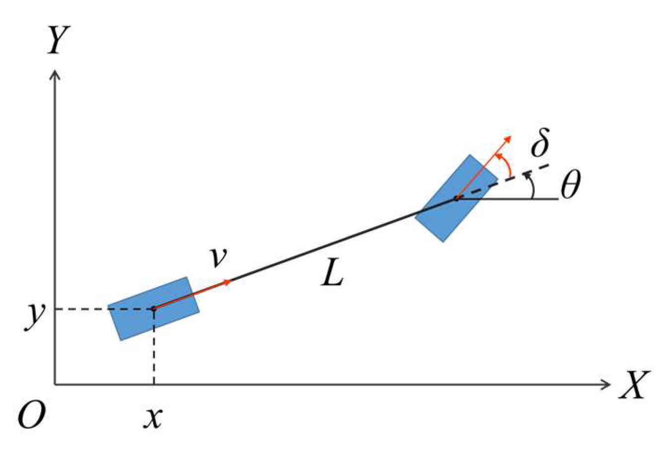
Figure 2.
Model-based Spatio-Temporal planning framework.
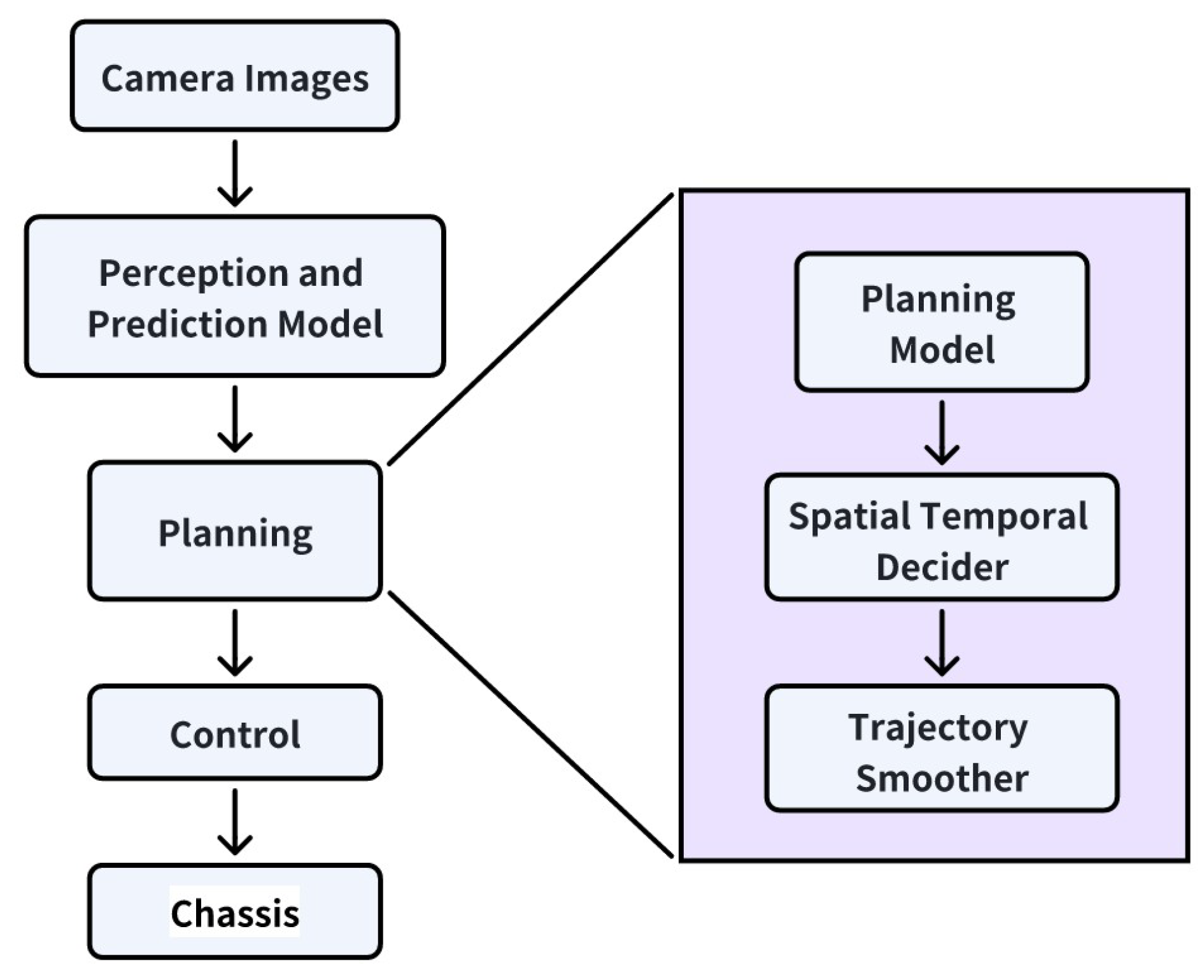
Figure 3.
Trajectory planning model framework.
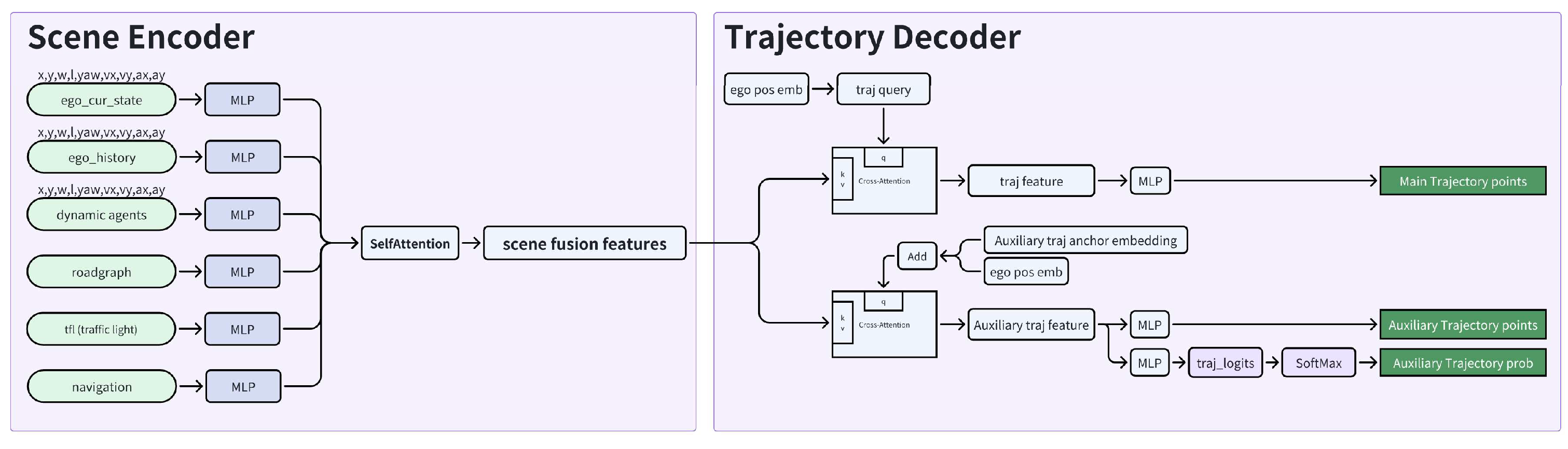
Figure 4.
An example of training pickle at intersection scenario.
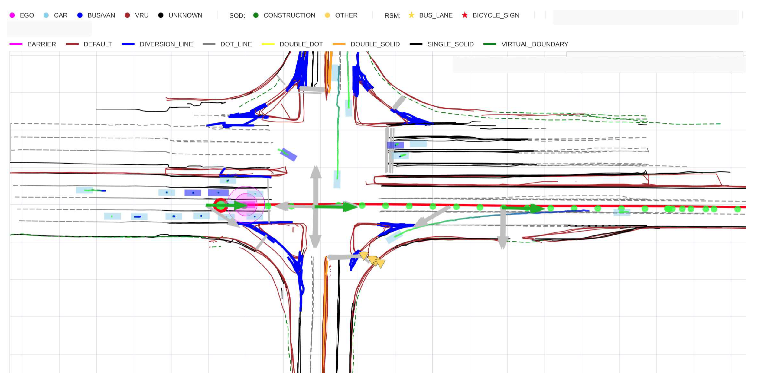
Figure 5.
Unprotected intersection scenario.
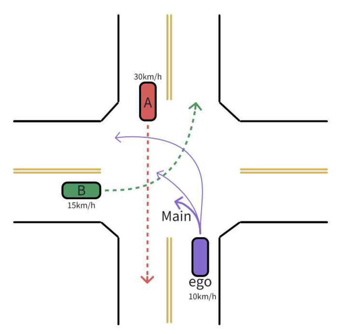
Figure 6.
Unprotected intersection scenario: ego-vehicle successfully avoids collisions with agents A and B via the selected main trajectory.
Figure 6.
Unprotected intersection scenario: ego-vehicle successfully avoids collisions with agents A and B via the selected main trajectory.
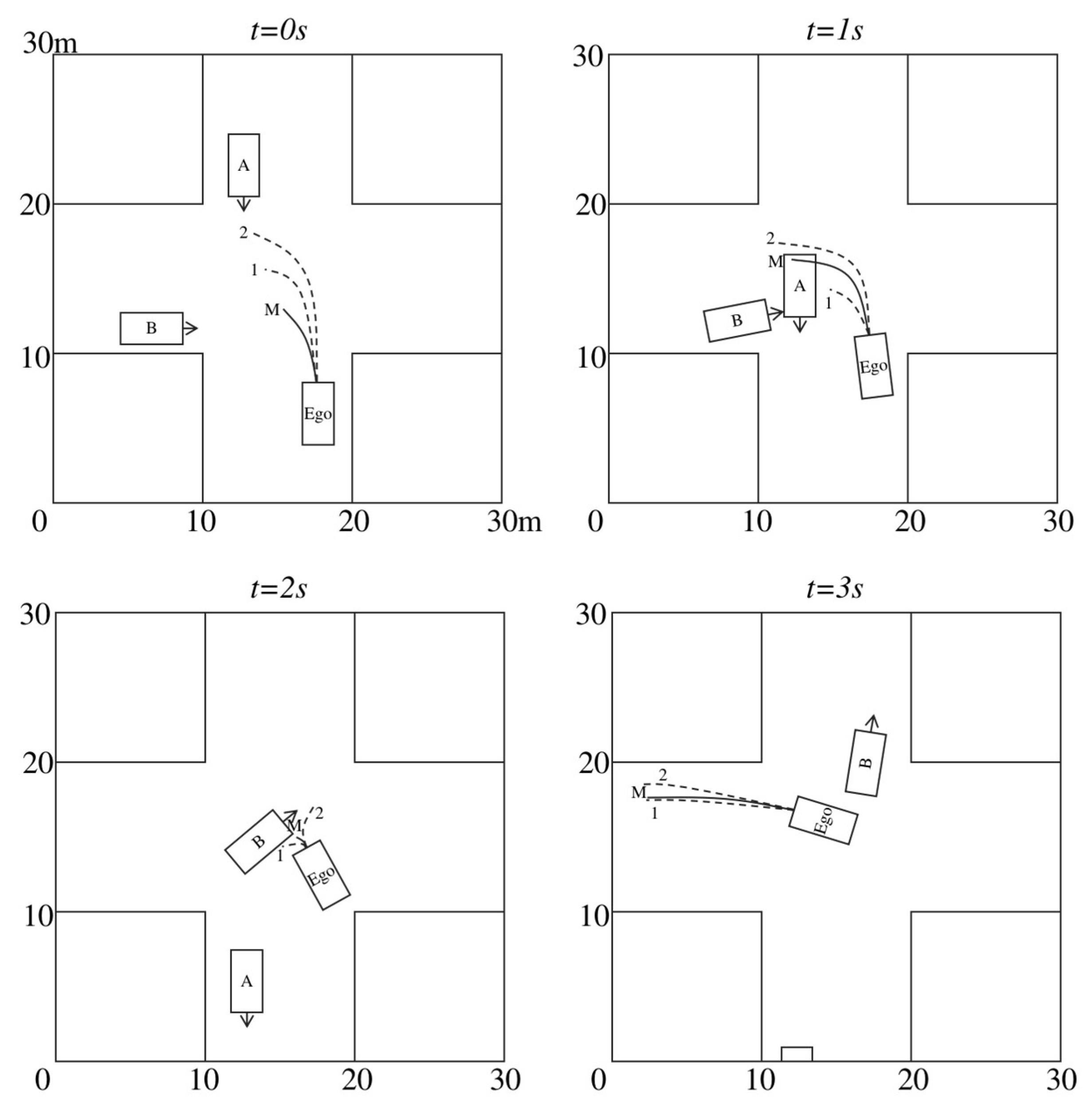
Figure 7.
Unprotected intersection: ego-vehicle successfully avoids collisions with other agents – screenshots from an on-dash test monitor.
Figure 7.
Unprotected intersection: ego-vehicle successfully avoids collisions with other agents – screenshots from an on-dash test monitor.
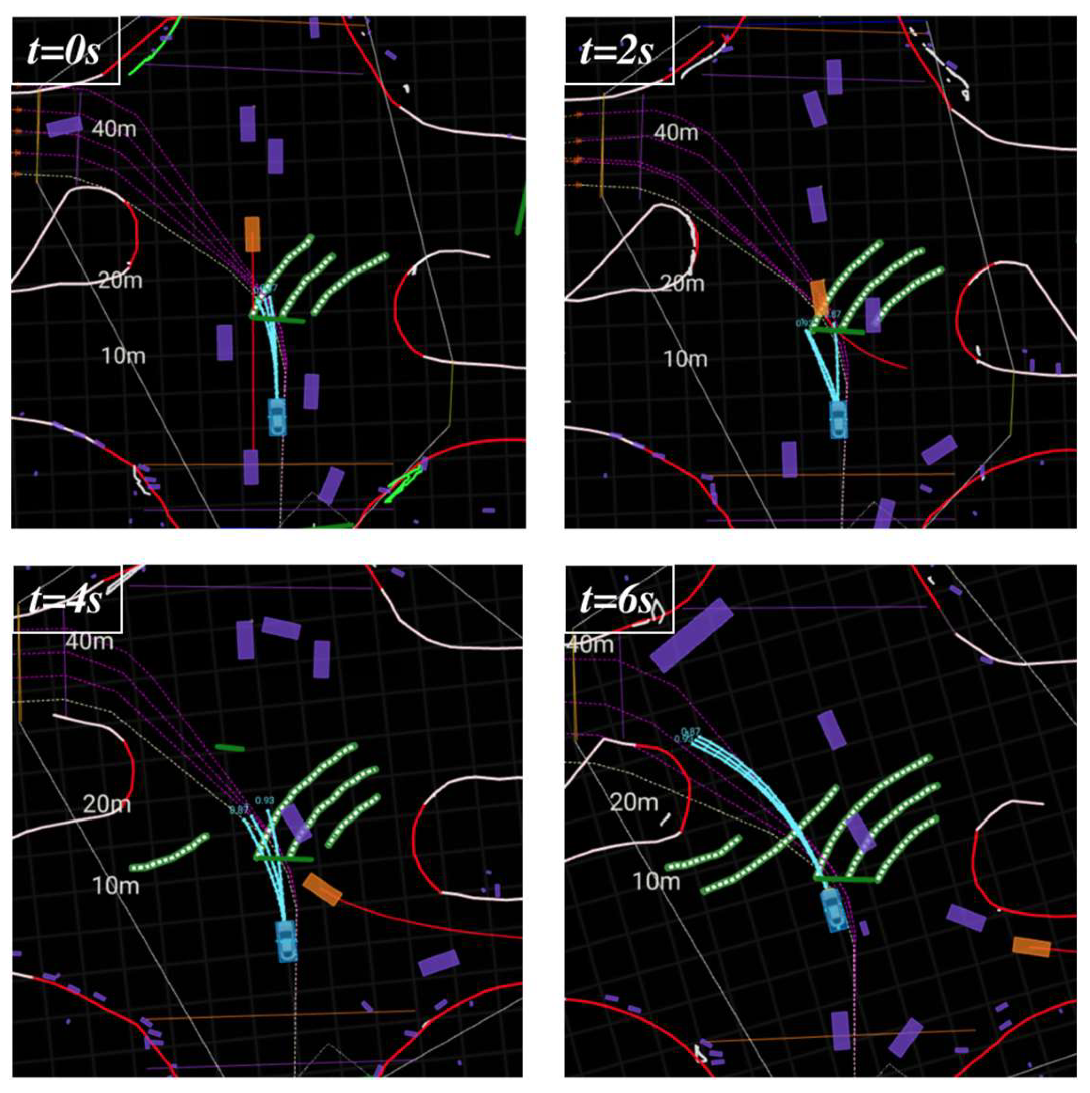
Figure 8.
Bypassing a slow-moving vehicle via the opposite lane in a narrow road.
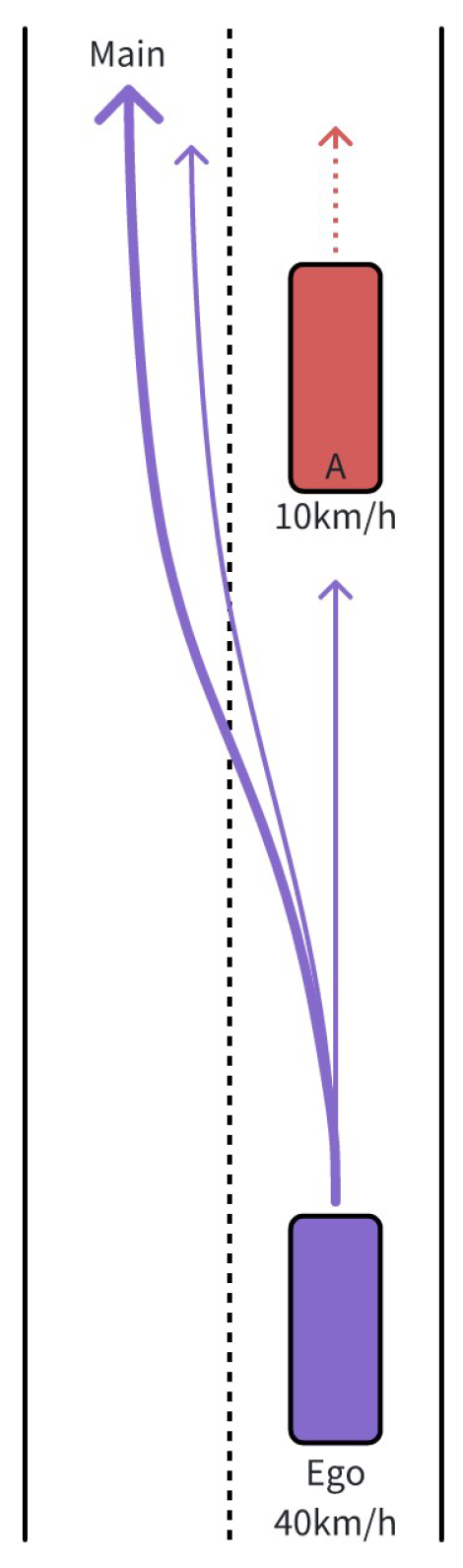
Figure 9.
To prioritize efficiency, the ego-vehicle bypasses the slow-moving vehicle on the narrow road by utilizing the opposite lane while maintaining safety.
Figure 9.
To prioritize efficiency, the ego-vehicle bypasses the slow-moving vehicle on the narrow road by utilizing the opposite lane while maintaining safety.
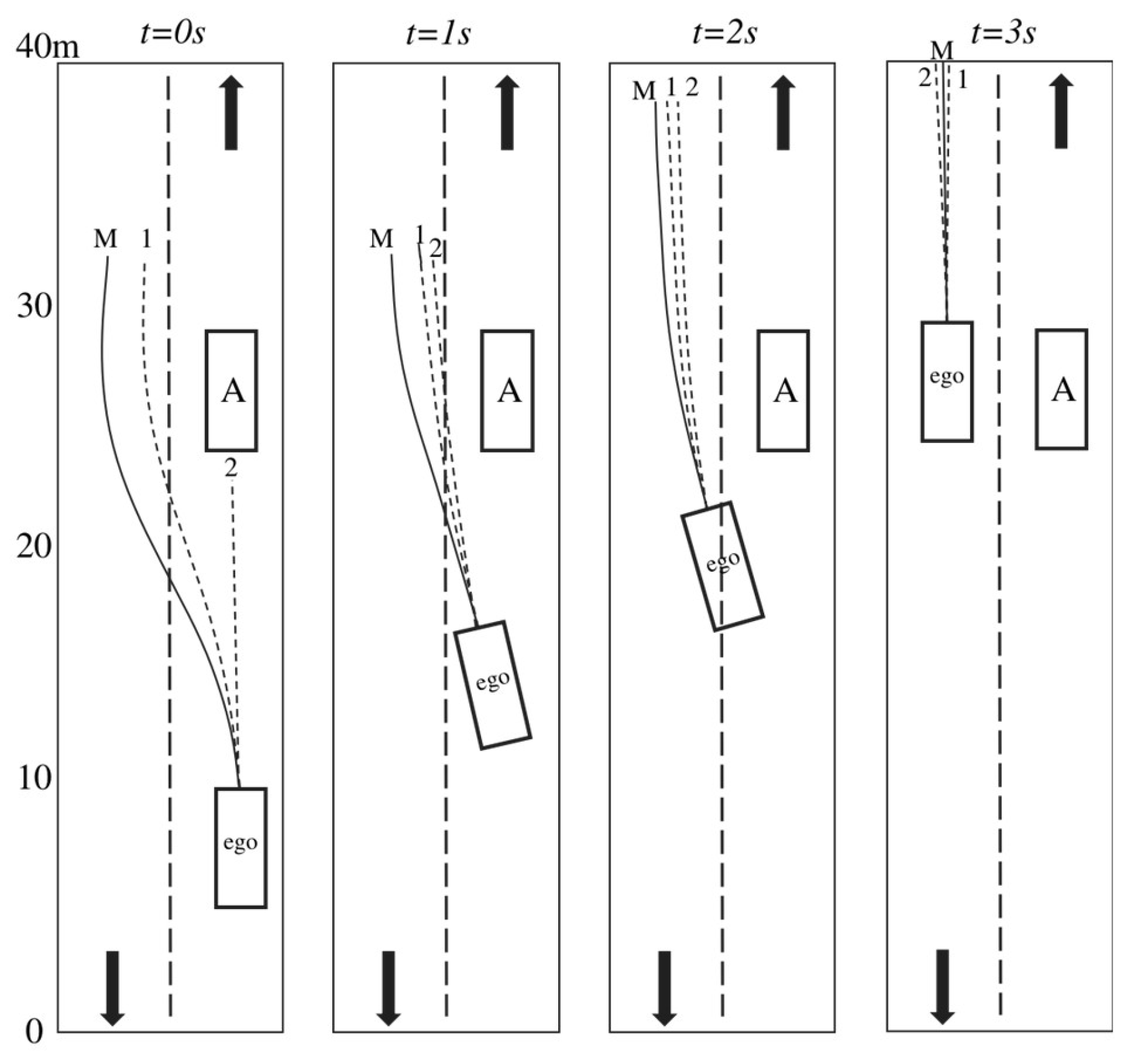
Figure 10.
Bypassing a stopped bus on a narrow road: ego-vehicle utilizes the opposite lane after it clears.
Figure 10.
Bypassing a stopped bus on a narrow road: ego-vehicle utilizes the opposite lane after it clears.
Disclaimer/Publisher’s Note: The statements, opinions and data contained in all publications are solely those of the individual author(s) and contributor(s) and not of MDPI and/or the editor(s). MDPI and/or the editor(s) disclaim responsibility for any injury to people or property resulting from any ideas, methods, instructions or products referred to in the content. |
© 2025 by the authors. Licensee MDPI, Basel, Switzerland. This article is an open access article distributed under the terms and conditions of the Creative Commons Attribution (CC BY) license (http://creativecommons.org/licenses/by/4.0/).
Copyright: This open access article is published under a Creative Commons CC BY 4.0 license, which permit the free download, distribution, and reuse, provided that the author and preprint are cited in any reuse.


