
Submitted:
14 November 2025
Posted:
17 November 2025
You are already at the latest version
Abstract
Accurate analysis of trace elements in particulate matter (PM) emitted by brake systems critically depends on the filter selection and handling processes, which can significantly impact analytical results due to contamination and elemental interference from filter elemental composition. This study systematically evaluated two widely used filter types, EMFAB (borosilicate glass microfiber reinforced with PTFE) and Teflon (PTFE), for their suitability in trace element determination of brake wear PM10 collected using a tribometer setup. A total of twenty-three PM10 samples were analyzed, encompassing two different friction materials, to thoroughly assess the performance and analytical implications of each filter type. Filters were tested for their chemical background, handling practicality, and potential contamination risk through extensive elemental analysis by inductively coupled plasma optical emission spectrometry (ICP-OES) and inductively coupled plasma mass spectrometry (ICP-MS). Additionally, morphological characterization of both filter types was conducted via scanning electron microscopy (SEM) coupled with energy-dispersive X-ray spectroscopy (EDS) to elucidate structural features affecting particles capture and subsequent analytical performance. Significant differences emerged between the two filters regarding elemental interferences: EMFAB filters exhibited substantial background contribution, particularly for alkali and alkaline earth metals (Ca, Na, Mg, and K), complicating accurate quantification at trace levels. Conversely, Teflon filters demonstrated considerably lower background but required careful manipulation due to their structural fragility and the necessity to remove supporting rings, potentially introducing analytical variability. Statistical analysis confirmed that the filter material significantly affects elemental quantification, particularly when the collected PM10 mass is limited, highlighting the importance of careful filter selection and handling procedures. Recommendations for optimal analytical practices are provided to minimize contamination risks and enhance reliability in trace element analysis of PM10 emissions. These findings contribute to refining analytical methodologies essential for accurate environmental monitoring and regulatory assessments of vehicular non-exhaust emissions.
Keywords:
metals
; particulate matter
; brakes
; brake wear particles
; ICP analysis
1. Introduction
Atmospheric particulate matter (PM) remains a major public-health and environmental concern, and in the last decades there is growing evidence of the role of non-exhaust traffic emissions alongside tailpipe sources [1,2,3]. Among non-exhaust contributors, brake wear particles are noteworthy for their complex metal signatures (e.g., Ba, Cu, Fe, Ti, Zn, Zr) and for their potential toxicological relevance in urban environment [4,5,6,7]. As brake wear particles (BWPs) are mainly inorganic, trace-element analysis is essential to reveal markers suitable for source apportionment of traffic-related PM. Literature reviews identified some gaps in the area of generation, detection, quantification and characterisation of airborne brake wear emissions [1,8]. The most critical issue related to these studies is the lack of standardized procedures. Another important gap is to find the best available techniques for sampling, quantitative measurement, and characterisation of brake wear particulate emissions. The chemical characterization of the PM emitted by different combinations of brake pads and discs, not only it allows to clearly and immediately assess their potential influence on environmental and health issues, but also to trace the different sources of atmospheric particulate matter through easier recognition of distinctive analyte patterns [2]. Reliable quantification of these elements is therefore essential for exposure assessment and mitigation strategies development.
Various instrumental techniques are employed to analyse the chemical composition of these emissions, each offering unique advantages: X-ray fluorescence (XRF) which enables rapid bulk elemental screening, Scanning Electron Microscopy (SEM) for studying morphology; X-Ray Diffraction (XRD) and Raman spectroscopy to identify molecular/phase information. [9,10,11]. [12,13,14,15,16,17,18,19].
In particular, Inductively Coupled Plasma - Optical Emission Spectroscopy and Mass Spectrometry (ICP-OES, ICP-MS) have gained attention for their ability to provide a detailed elemental analysis of brake wear particles. ICP-OES and ICP-MS are highly sensitive and capable of detecting major, minor, trace (ICP-OES) and ultra-trace (ICP-MS) elements in complex matrices, making it a powerful tool for quantifying inorganic elements in brake wear emissions [19,20,21]. However, the sample preparation is time-consuming and their use is less frequent compared to XRF and SEM-EDX for BWPs characterization, so far. Despite this, studies have demonstrated the effectiveness of these techniques in quantifying metal concentrations in road dust and brake wear emissions [22,23].
Sample preparation for ICP-OES and ICP-MS analysis usually requires acid dissolution of the solid samples, for instance by the use of microwave-assisted digestion to accelerate and optimise sample dissolution, thereby improving recovery rates for element analysis [24,25,26]. However, the correct selection of the type of acid used in the process is fundamental to obtain accurate results. Different acid mixtures are used in the procedures for PM10 digestion depending on the sample composition and elements of interest. Nitric acid (HNO₃) is widely used for this purpose. It can oxidize organic matter and most inorganic compounds, although some metals are passivated (e.g. Al, Cr, Ti) [24,27]. The combination of HNO3 with hydrochloric acid (HCl), especially in the proportion 1:3 (aqua regia), enhances the dissolution of metals and metal oxides [27,28]. Hydrogen peroxide (H₂O₂) can be used to improve digestion efficiency, particularly for samples with high organic matter content. The mixture HNO3:H2O2 (4:1 ratio) is the acid mixture reported in the digestion method for the determination of Pb, Cd, As, and Ni in PM10 standardised by the European Directive 2004/107/EC (UNI EN 14902:2005) [29,30,31,32]. Sometimes the mixture HNO3/HF/H3BO3 is also used, though less frequently due to the hazardous nature of hydrofluoric acid [22,33,34,35]. Indeed, HF is a weak acid that behaves as a strong complexing agent. It forms stable fluorides and fluorine complexes with many elements, enabling the dissolution of refractory species (e.g., silicates). H3BO3 (boric acid) is used to reduce the possible presence of excess HF in solution by forming HBF3OH.
Overall ICP-OES and ICP-MS provides highly accurate elemental quantification while XRF is preferred for rapid and non-destructive elemental analysis, and SEM-EDX is essential for morphological studies. Given these premises, the integration of several analytical techniques remains the most effective approach to gain a comprehensive understanding of brake wear emissions and their environmental impact.
In this work, innovative acid mixtures were tested to obtain the complete dissolution of PM samples using a single acid mixture. Fluoroboric acid (HBF₄) has emerged as a powerful alternative to hydrofluoric acid (HF) in the acid digestion of siliceous and refractory materials. The replacement of HF is highly desirable due to its acute toxicity, volatility, and corrosiveness, as well as its tendency to produce insoluble metal fluorides (e.g., CaF₂, MgF₂, AlF₃, Rare Earths Elements fluorides), which can impair elemental recoveries and damage analytical instrumentation. HBF₄ circumvents many of these issues by acting as a moderated source of fluoride ions, undergoing stepwise hydrolysis in aqueous solution [36].
These steps ensure the progressive release of fluoride under acidic conditions. Unlike pure HF, which often requires post-digestion neutralization with boric acid to prevent SiF₄ volatilization or metal-fluoride precipitation, HBF₄ offers an intrinsically buffered medium (due to the presence of boron-oxygen), especially when combined with HNO₃ [37,38,39].
In terms of analytical performance, several studies have demonstrated that HBF₄ based digestion methods can match or even exceed HF-based methods, especially for multi-elemental analysis of silicon-rich or mineral matrices such as soil, sediments, or particulate matter [37,39,40].
While optimized acid mixtures are decisive for complete dissolution and recovery of the analytes, the substrate onto which particles are collected is equally determinative for achieving accurate results. The recent protocol “Minimum Specifications for Measuring and Characterizing Brake Emissions” edited by the Particle Measurement Program Informal Working Group (Task Force 2 – Brake dust Sampling and Measurement) in July 2021 recommended PTFE-coated glass microfiber (EMFAB) and PTFE membrane filters with polymer support as filter material for brake wear PM collection in the context of brake homologation tests carried out by dynamometer bench test, specifically to measure gravimetrically brake particle emissions [41]. EMFAB filters consist of borosilicate glass microfibers reinforced with woven glass cloth and bonded with PTFE and offer greater mechanical robustness and airflow for gravimetry and handling, but their glass-fiber composition can contribute to alkali/alkaline-earth background or interact with aggressive acid digests, so the control of the background contribution is more critical [42].
PTFE filters are chemically inert and consistently show the lowest elemental blanks, which is why they are preferred for trace-element determinations; but the main practical issue is related to the polymethylpentene (PMP) ring that support the filter and this can complicate sectioning and digestion processes [43,44].
From these insights, our study systematically evaluates EMFAB and PTFE filters for trace-element analysis of brake-wear PM₁₀ generated on a tribometer system. We (i) test new acid mixtures using HBF4 and validate the results using certified reference materials (NIST 1648 a, BCR 176), (ii) quantify and compare filter backgrounds, handling practicality, morphology, and contamination risk via ICP-OES, ICP-MS and SEM-EDS; (iii) test internal and external-standard calibration strategies in ICP-MS to minimize matrix- and instrumental drift-related bias, (iv) analyze brake wear PM10 collected on EMFAB and PTFE filters from two pad/disc formulations (non-asbestos organic (NAO) and low-steel (LS) tested with gray cast iron discs) through a tribometer system. The goal is to deliver practical recommendations on filter selection and analysis (digestion and calibration) protocols that enhance data reliability in trace-element analysis of non-exhaust particulate emissions.
2. Results
1.1. Sample Pretreatment Results
The average recoveries, expressed as percentages, obtained for the nineteen elements with their standard deviations from the analysis of Standard Reference Material NIST 1648a with the mixtures A, AO, B and BO are shown in Figure 1.
Comparing mixture A (HNO3 + HBF3) and mixture AO (A Overnight), a paired-sample t-test (α=0.05) found no significant differences, except for Si (p-value = 0.025), which was a higher value with A (70%) than with AO (59%). Conversely, for mixture B (HNO3 + HBF3 + H2O2) and BO (B Overnight), recoveries differed significantly for Al, Ca, Fe, Si, V, Co, Ni, As, Cd and Pb Al, Ca, Fe and Si were higher (p-values in Supplementary Table 2) with B (respectively, 142%, 130%, 165%, 92%) than with BO (respectively, 74%, 73%, 83%, 71). For V, Co, Ni, As, Cd and Pb, recoveries were generally higher with BO (200%, 189%, 202%, 239%, 194%, respectively) than with B (115%, 127%, 131%, 180%, 149%, 133%). Recoveries above 115% (see Supplementary Table 1 for acceptance criteria) flag suspect results that may arise from the mixture and the 16-h contact time and/or ICP-MS interferences. If we consider the average of the relative standard deviations (RSD%) of the element’s recoveries per mixture, we noticed a 3% for mixture A in contrast with 12% with AO and 22% for B in respect of mixture BO (24%). Therefore, we excluded the overnight conditions from the suitable choice of attack digestion for PM10 samples.
To compare mixtures A, B and C, Table 1 reports mean recoveries alongside AOAC acceptance ranges (which depend on the SRM analyte concentration) and Horwitz ratios for repeatability (HORRATr, as defined in Eq.2, in paragraph 3. Materials and Methods) values, with an acceptance range of 0.5–2 [45].
Mixture A places 13/19 analytes within the AOAC acceptance window, with four clear fails below 80% (notably, Ti 76%, Cr 53%, Al 62% and Si 72%). Precision is consistently acceptable: HORRATr falls within 0.5-2 for 15/19 analytes, with only Ca, Si, Cr exceeding 3 and V below the lower limit. By contrast, mixture B shows a systematic positive bias: only 10/19 analytes lie in the 80–115% window, while many exceed 125%—e.g., Co 127%, Al 128%, Ni 131%, Pb 133%, Fe 148%, Cd 149% and As 180%, This inflation in B is mirrored by poor repeatability: only 7/19 HORRATr values are in the range 0.5-2. Most fall in the 5–11 range, with a few borderline cases around 2.4–2.8 (Ti, Cr, Co). Finally, mixture C exhibited 9/19 analytes with acceptable recoveries, the lowest result among all mixtures. At least six elements reached values below 50% (K 47%, Na 44%, Al 39%, Cr 33%, Ti 19% and Si 1%). Considering repeatability, mixture C performs better than B with 12/19 elements in the 0.5-2 acceptable values.
In summary, mixture A (4 mL HNO3 + 2 mL HBF4) provides more consistent precision and adequate accuracy for most elements. Besides, HBF4 confirms to increase the solubilization of refractory elements such as Ti, K, Al and Na that could be occluded in silicate fraction and increased also the solubilization of Cr and Si itself.
The percentage recoveries obtained using the acid mixtures A and Amodified (mixture A with the addition of 2 mL of HPW) and two different heating programs in microwave oven are shown in Supplementary Figure 1. We observe a statistically significant difference (paired samples t-test) for Mg, K, Ti, Cu, Al and Si. Only for Ti and Al the addition of 2 mL of HPW has a positive effect (105%, 80% and 76%, 62% as percentage recoveries for mixture Amodified and A, respectively). As could be expected, the addition of HPW dilutes the acidity and the effective concentrations of the species F-/HF (generated from HBF4) leading mainly to slowing the dissolution of silicate/oxide phases affecting the efficiency [46]. Not only, but probably the slower kinetics could amplify small differences in sample load, volumes and local temperature during digestion leading to uneven degrees of dissolution across replicates, confirmed by the higher standard deviations obtained by all analytes for mixture Amodified.
We also evaluated two strategies for signal drift-correction in ICP-MS: internal-standard normalization (89Y, 115In, 125Te, 193Ir) and external calibration with intermittent reads of one calibration standard following a bracketing design (EST). To test whether any internal standard provided a measurable advantage, we used a one-factor ANOVA and reported least-squares means (LS, model-adjusted means). The factor was not significant (p = 0.261), and Tukey HSD post-hoc test found no pairwise differences among groups; LS-means clustered tightly (193Ir ≈ 93.1%, 89Y ≈ 91.1%, EST ≈ 89.3%, 115In ≈ 87.5%, 125Te ≈ 87.1). Considering these results, we preferred to adopt EST strategy for signal drift-correction, simplifying the workflow and avoiding potential contamination from spiking internal standards. Supplementary Figure 2 and Supplementary Table 3 show the % recoveries obtained for the isotopes by the different drift corrections approaches and the outcomes of the post-hoc Tukey HSD test.
Finally, we tested mixture A on a second standard reference material (BCR-176, fly ash) to evaluate its applicability on samples of different matrices. Table 2 reports mean percentage recoveries and HORRATr values.
Overall, BCR-176 shows generally acceptable accuracy and repeatability. Most targets fall in the AOAC percentage recovery window with HORRATr between 0.5 and 2. For example: Mn 90% (1.2), Fe 91% (0.9), Na 101% (1.5), Zn 88% (1.1), Ba 94% (0.9), Cu 103% (0.5), V 109% (0.6), Ni 104% (1.5), As 97% (1.9), and Pb 103% (1.0). Cr performs well with an average recovery of 78% (HORRATr: 1.2) not far to the acceptable AOAC value of 90%. In stark contrast, the use of the same mixture A in the NIST 1648a showed decreased Cr (53%,) and higher HORRATr (2.1), underscoring a matrix-dependent difference in extractability. A plausible matrix-driven explanation is that, in fly ash, Cr is predominantly hosted in phases that are efficiently attacked by the HNO₃–HBF₄ mixture, namely glassy aluminosilicates and Fe-oxide/spinel domains typical of combustion ash [47,48]. Under these conditions HF/F- generated from HBF₄ dissolves silica-rich glass via hexafluorosilicate formation (e.g., [SiF₆]2⁻), promotes the dissolution of Al-rich frameworks, and stabilizes metal–fluoro complexes (e.g., [CrF₆]3⁻), facilitating Cr release [49]. In contrast, a larger fraction of Cr in NIST 1648a is plausibly associated with more refractory metal-rich particles, chromite-like spinels, or carbonaceous matrices that digest less completely under the same conditions; thus, recovery remains lower even though the bulk “silicate percentage” of the two SRMs is comparable (around 30%) [50]. Javed et al. (2020) and Zimmermann et al. (2020) developed digestion methods based on mixtures that comprise nitric acid and fluoroboric acid for the analysis of soil and sediment samples. Their results yielded high recovery rates for elements that are typically difficult to solubilize, including aluminium, chromium, potassium, titanium, and silicon including also zirconium and molybdenum (Zr and Mo silicon in the range of 85-100% (Zr and Mo could not be compared in this work because they are not present in the tested SRMs samples) [37,40].
1.1. Tribometer/Dynamometer PM10 Sample Comparison
To evaluate the consistency between the novel tribometer set-up and the reference dynamometric bench in terms of PM10 chemical composition, it was compared the chemical composition of PM10 emitted by the wear of a tribological couple composed by GCI disc and NAO pads and collected on EMFAB filter on dynamometer bench (one single test was performed) and the average chemical composition obtained for NET samples (five tests obtaineid with EMFAB filters on the tribometer with the same friction material and GCI disc). Figure 2 shows the percentage concentrations of the determined elements above the total mass of PM10 collected by the two set-ups (tribometer and dynamometer). See also Supplementary Table 4 for the exact values.
A pearson correlation was calculated obtaining a p-value <0.0001 with a positive correlation of 0.991. While many elements showed good agreement between the two systems and include Fe, Zn, Zr, Ti, Ba, Sn for major elements but also Cu, Mn, Mo for trace elements; elements, like K, Mg, Sr and Al, have not been quantified in tribometer tests for two different reasons: Al, Mg and Sr concentrations in the PM10 were overwhelmed by the sample blank, whereas K had percentage concentrations higher than 120% probably due to some unknown contamination, therefore, K was excluded. Hence, these four elements are easily traceable to the filter contribution. A key difference observed between the dynamometer and the tribometer concerns the total mass of PM10 collected during testing. In the case of NAO friction material, the dynamometer test, lasting approximately 36 hours, allowed for the collection of a larger quantity of PM10, accounting for 1.65 mg, compared to an average of only 0.5 mg collected during tribometer tests after 10 hours.
Overall, the data suggest a good correlation between the two set-ups, with the tribometer capable of capturing the main chemical emission profiles but also showing some degree of bias for certain elements due probably to the high contribution of EMFAB filter, that require the collection of high amount of material. This result highligths the need to investigate the use of different types of filter material.
1.1. Filter Blanks Comparison
Figure 3 shows the morphology of the two types of filters investigated with their relative composition obtained by EDS spectra. EMFAB filter reveals a chaotic, randomly oriented fibrous network. The fibers appear to be intertwined in a highly porous 3D structure, which is typical of filters made of glass wool. The random fibers arrangement and high porosity could likely facilitate particles capture by interception and impaction. The higher magnification (Figure 3b) clearly shows thin, smooth, and uniform glass fibers with diameters in the sub-micron to low micron range. This filter’s morphology is well-suited for collecting airborne particles of various sizes due to the dense yet porous fibrous mesh. The random orientation maximizes contact with particles suspended in air. EDS results highlight the complex chemical composition, confirmed also by ICP analysis (Supplementary Table 5): F and C can be traced back to the presence of the teflon part of the EMFAB filter whereas the high presence of Si (11%) followed by Na, Ba, Zn, Al, K and Ca (summed to 9%) are associated with the presence of borosilicate glass fibers. The presence of these elements in high amount in the filter’s background underline the difficulty of the right quantification of these analytes in the PM collected. For instance, the higher contribution of Si in the filter makes extremely difficult its quantification in PM10 samples and to disentangle whether Si comes from PM or from the filter even after substracting a mean value of concentration in the blank filter.
PTFE filter surface displays a much more regular and compact structure, with a discernible grid-like or textured pattern (Figure 3c). Unlike EMFAB filter, it lacks the fluffy, fibrous appearance and appears smoother and more compressed. At higher magnification (Figure 3d), the surface turns out to be composed of finer fibrous elements, but these fibers are embedded in a more compact, potentially layered structure. Its finer pores and smooth surface may allow for more efficient capture of particles by diffusion. EDS spectra confirm that the composition is made of F (72%) and C (28%).
To mitigate the risk of losing of collected PM from PTFE filter during the PMP ring removal processes, the filters were covered with paper tape. In Supplementary Figure 3 is showed the concentration obtained by the digestion of a commercial paper tape. Adhesive tape showed lower concentrations therefore appears to be the best due to the lower content of almost all the elements investigated except for Ti, which highlights a contribution of 0.5% of the total mass of tape digested that could affect the right quantification of this element in the PM10. Despite this additional step, the concentrations of the elements present in the blank PTFE filter covered by the adhesive tape are much lower for all elements by at least 1 order of magnitude in respect of EMFAB ones, except for Ti, Cu and Pb (Figure 4). For Cu, PM10 concentrations in the samples were consistently about one order of magnitude higher than the corresponding PTFE blank value, in contrast, Pb was of the same order of sample concentrations, so its quantification was more susceptible to blank bias.
Finally, a greater reproducibility of the results was observed with the PTFE filters covered by the tape than with the EMFAB filters. Concentration values can be seen in Supplementary Tables 6.
1.1. PM10 Samples Results
A Principal Component Analysis (PCA) was applied (Figure 5a) to the dataset composed by the elemental composition of the twenty-three PM10 samples collected on EMFAB and PTFE filters.
The first two principal components explain 62.67% of the total variance and show a clear differentiation between the PM10 samples according to the type of friction material. LS-derived samples (LET and LTT) cluster, in the lower left part of the score plot, is characterised by negative values of PC1 and PC2, while NAO-derived samples (NET and NTT) occupy mainly the upper region, characterised by positive values of PC2. A striking observation is that the difference between EMFAB (NET) and PTFE (NTT) filters appears only in NAO samples with high positive values of PC1 that grouped NET samples, whereas NTT samples are mainly characterised by negative values of PC1. Moreover, it is possible to evidence a separation also between the NTT samples with paper tape that adhere to the bottom side of the filter (NTT-B) and NTT samples with paper tape that seals the PM collected on the top side of the filter (NTT-T). This is likely due to the incomplete effectiveness of the tape placed on the bottom side of the filter in preventing partial loss of the PM during the PMP ring elimination phase. This led to a greater dispersion of the NTT-B samples and an underestimation of the element concentrations in the PM collected. Finally, the greater dispersion and separation for NAO samples can be explained by the very low mass of collected PM10 (always below 1 mg for the thirteen PM10 samples obtained by NAO brake pads wear), making the analysis more sensitive to variability and potentially less accurate due to the greater influence of the chemical composition of the filter itself and of the analytical preparation.
LS samples (LET and LTT) cluster tightly regardless of the filter type, indicating that the filter material does not significantly affect the results when PM mass is sufficiently high (7-16 mg). This suggests that for low-mass samples, such as those from NAO materials, the choice of the filter is critical for obtaining reliable compositional data, while for LS samples, the higher PM mass reduces the influence of the filter type.
The loading plot (Figure 5b) clarifies how the two components are characterized by the variables. PC1 is driven positively by Cu, Ni, Co, Cd, Cr, Mn, Sn and K and negatively by Fe, V and, to a lesser extent, Al and Sr. PC2 separates Ca, Ti, Zr and Ba (together with mildly positive Na, Mg, Zn, Pb, Mo) on the positive side from Mn–Cu–Ni–Co on the negative side. Accordingly, NET samples with high positive PC1 scores align with the Cu–Ni–Co–Cr–Mn vector, whereas the negative PC1 scores of LS-samples point toward the Fe–V direction. The positive PC2 values of most NAO samples are consistent with Ca-Ti-Zr-Ba-rich formulations (typical barite, calcium carbonate, potassium titanate, zirconium oxides/silicates), while the negative PC2 values of LS samples reflects the stronger Fe, Al and V signature expected for low-steel materials (due to alumina, metallic Fe, steel) [1,51].
Applying Hierarchal Cluster Analysis (Supplementary Figure 4), the whole of the information of the dataset is considered. Two clusters , one composed by NET samples and the other composed of LS (LET and LTT) and NTT samples respectively are obtained. At a lower dissimilarity level LET and LTT separates from NTT samples forming two distinct sub-clusters. Again NET and NTT samples show an higher dissimilarity being at the extremes of the dendrogram underlining the greater influence of the type of filter in NAO samples.
To further investigate whether the filter material (EMFAB vs. PTFE) or the different analytical procedure (sealing the PM10 with tape on the bottom or on the top of the filter) influences the chemical composition of the PM10 samples, non-parametric Kruskal-Wallis test was applied to three different groups of samples: 1) LET and LTT; 2) NET and NTT; 3) NTT-T and NTT-B. This statistical approach was chosen due to the small sample size of the groups and the large number of variables considered. A significance level of α = 0.01 was selected intentionally to minimize the risk of committing a Type I error, thereby increasing the statistical stringency in detecting true differences among the groups. The p-values obtained for each element considering the three aforementioned groups are showed in Figure 6. Kruskal-Wallis results for LET and LTT samples reveal that several elements exhibit statistically significant differences depending on the types of filter. Notably, Al, Ba, Ca, Cd, K, Mg, Na, and Sr show p-values below 0.01, indicating strong evidence that their concentrations vary depending on the filter material. Except for Cd, all these elements are found in EMFAB filter.
For the second group tested (NET vs NTT), Ca, Co, Cr, K, Mn, Ni and Ti show a statistically significant difference between the two types of filter. In this case we find elements, such as Ca and K, that already differentiated the two different filter types. The difference found for Ti could be traced back to its presence in the tape used for PTFE filters. Although this difference was not shown in group 1, it must be remembered that the samples obtained from the NAO pads wear were characterized by very low mass concentrations and this can affect the result in different ways. Importantly, the total mass of PM10 collected in the two different groups tested did not differ significantly between EMFAB and PTFE filters indicating that the observed chemical differences are not due to systematic differences in mass concentration collected. Finally, NTT-T and NTT-B samples do not show statistically significant differences at selected significance level suggesting that the sealing process itself does not introduce a different chemical bias in the elements distribution in PM collected on PTFE filters. The difference between these two groups can be seen for higher significance level (α ≥ 0.05).
To assess both the analytical precision and the repeatability of the elemental concentration measurements, intra-sample and inter-sample relative standard deviations (RSD%) were calculated for each sample category. For each filter, the sample was physically divided into two halves, and each half was analyzed separately. The intra-sample RSD% was calculated for each element based on the two replicates. Finally, an overall RSD% value for each category (filter, brake pad and with tape on bottom or top) was obtained by averaging the RSD% values obtained as intra-sample... This metric reflects the sampling homogeneity of the tribometric setup and analytical procedure applied to a single sample. The second type of RSD%, defined as inter-sample RSD%, quantifies the repeatability across different samples within the same category. For each element, the RSD% was calculated using the concentration values obtained from each filter belonging to the same experimental group. Subsequently, a global RSD% value for the category was obtained by averaging the RSD% values of all the determined elements. This second approach highlights the natural variability among different filters and represents the overall consistency of the PM10 collection and analysis process within each category.
The intra- and inter-sample RSD% values calculated for each experimental category are summarized in Table 3.
The intra-sample RSD% shows a better sampling homogeneity for LS filters (8% and 7% for LET and LTT, respectively).. For NAO groups, a intra-sample RSD% of 10% was obtained by NET group. NTTs groups show a lower sampling homogeneity. In general PTFE filters were more manipulated for removing the PMP support ring and this impacts more when the quantity of PM to analyse is very low. Precision seems to improve slightly by sealing the PM10 with tape on the top (15% NTT-T) in respect on the bottom (18% NTT-B). Inter-sample RSD% revealed a broader range of values, from 20% (LTT) to 50% (NET). The highest inter-sample variability in NET samples may be attributed to the lower total PM10 mass collected. On the other hand, LS samples (LET and LTT) exhibited the lowest inter-filter RSD%, confirming the overall stability and repeatiblity of PM10 composition. Interestingly, the sealed NTT-T samples also showed reduced inter-filter variability (24%) compared to NTT-B samples (41%).
3. Materials and Methods
1.1. PM10 Tribometer Samples
Twenty-three PM10 samples were analysed (Figure 7).
Ten samples have been obtained using a Low-Steel (LS) friction material tested with gray cast iron disc (GCI), a half collected with EMFAB filter (named as LET) and the other half with PTFE filter (named as LTT). Thirteen samples have been obtained using Non-Asbestos Organic (NAO) friction material tested with GCI discs, five with EMFAB filter (NET) and eight with PTFE filter (NTT). Of the eight NTT samples, five were with paper tape that adhere to the bottom side of the filter (NTT-B) whereas three were with paper tape that seals the PM collected on the top side of the filter (NTT-T).
Samples name, type of friction material, type of filter, and PM10 mass collected are shown in Table 4.
1.1. Tribometer Set-Up
The tribometer model used was a Bruker UMT-TriboLab. This device is composed of two main parts: a rotor in the lower part, which simulates the rotating disc of the brake system, and a carriage, free to move in the Z-axis direction, on which the brake pad samples reside and most of the sensors are mounted.
The brake pad samples are fixed inside a sample holder: three samples of brake pad materials are needed in order to have a stable support and to better distribute the pressure. The brake pad samples are obtained directly from a finished brake pad: the friction material is mechanically detached from the pad backplate, the thickness is set to 7.5 mm with a flat-surface grinding machine and lastly samples of 1 cm by 1 cm area are created using a cutting machine. Tribometer discs are directly obtained from Heavy Duty truck GCI, cut with a final diameter of 9.5 cm. Thanks to this device it is possible to define a brake procedure made up of several brakes defined by set values of sliding speed, brake time, deceleration and load force. The acquisition rate at which the instrument measures each quantity is 10 Hz. A Worldwide Harmonized Light Vehicles Test Procedure (WLTP) simulation on the tribometer was developed to replicate the official WLTP used on a chassis brake dynamometer, adapting it to the different scale and working principle. The procedure consisted of 303 individual braking events divided into 10 consecutive trips characterised by increasing average speeds. Between the individual trips, a stationary time (approx. 10 minutes) is required to cool the braking system and reach an ambient temperature. The total duration of the test is 10 hours.
For the quantification and inorganic characterisation of PM10, a stainless-steel chamber was designed to be able to convey the particulate matter emitted by the brake system during the WLTP simulation tests onto a filter. The set-up developed for the collection of the PM10 fraction is schematically represented in Figure 8.
The compressed air injector serves to have a greater inlet flow so as to create a slight overpressure inside the chamber. The air, before entering the chamber, is purified through a HEPA Capsule Versapor™ filter that guarantees 99.97% retention of particulate matter having equivalent aerodynamic diameter of 0.3 μm. The purified air flow passes into the chamber where the wear of the friction material occurs, PM of various sizes is formed and conveyed outside the chamber to the Dekati cyclone. The latter is made entirely of stainless steel and is used to remove large particles (>10 µm) from an aerosol stream before the sample reaches the sampling filter. The cyclone is manufactured according to EPA standard 201A. The fraction of PM10 selected by the cyclone passes through the filter holder and settles on the selected filter. The air flow is conveyed to the dehumidifier, and the flow rate can be controlled through a flow meter. The entire system is connected to a rotary pump (10 L/min), which enables the air flow to transport the particulate matter and convey the PM10 fraction to the sampling filter. Tests were conducted on 47 mm diameter EMFAB and 47 mm diameter PTFE filters. Each filter was weighed before and after the test using an analytical balance (readability 0.1 mg), and the gravimetric mass was obtained by difference.
1.1. Sampling Filter Blanks
In the evaluation of the suitable filter for PM10 collection, the inorganic chemical composition of the different types of filters was considered. Three EMFAB and three PTFE filters were cut in two and analysed with the mixture chosen according to the procedure described below. The average values of the concentrations of the filters were subtracted from the concentration of the samples, in order to eliminate the contribution of the filter. PTFE filters have a PMP (polymethylpentene) ring, which is incompatible with the acid digestion procedure because of the highly exothermic reaction of this material with the selected acid attack mixture, and the uncontrollable overpressure of the system with the risk of vessel explosion. To resolve this situation, it was decided to remove the PMP support before proceeding with the digestion of the samples. However, removing the PMP support proved to be a complicated task due to the risk of losing collected material during the manipulation. It was concluded that the best solution was to adhere the filter to a paper tape base. This solution effectively immobilised the PTFE filter mesh, preventing it from wrinkling during cutting and ensuring more accurate sample preparation. To obtain reliable concentration values for the sample blank the PTFE filter stuck together with the paper tape was analysed.
1.1. Reagents
Reagents were all of analytical purity. Water was purified in a Milli-Q system, resulting in high purity water (HPW) with a resistivity of 18.2 MΩ∙cm. Intermediate metal standard solutions were prepared from concentrated (1000 mg/L) stock solutions (CPI International) and acidified to pH=1.5 with nitric acid. HNO3 ≥65%, HBF4 48%, were purchased from Sigma-Aldrich, H2O2 30% from VWR Chemicals.
1.1. Sample Pretreatment
Three acid mixtures were tested in this work: one consisting of 4 mL HNO3 and 2 mL HBF4 (mixture A) the second one consisting of 4 mL HNO3, 1 mL HBF4 and 1 mL H2O2 (mixture B) and the last one composed by 4 mL of HNO3 and 1 mL of H2O2 (mixture C) Furthermore, to assess the effect of increased contact time, additional tests were carried out where mixtures A and B remained in contact with the certified sample for 16 hours (AO, BO).
To evaluate the efficiency of the extraction procedure, it was necessary to evaluate the recoveries of the analytes chosen through the analysis of a standard reference material (SRM). The standard reference material 1648a (Urban Particulate Matter) was used. Once the best mixture was chosen, another standard reference material, namely BCR 176 (Fly Ash). Al, Ca, Cd, Co, Cr, Cu, Fe, K, Mg, Mn, Na, Ni, Pb, Si, Sr, Ti, V and Zn were the certified elements present and determined in SRM NIST 1648a, whereas Ba, Cr, Cu, Fe, Mn, Na, Ni, Pb and Zn were the analytes determined in SRM BCR 176.
Fifteen replicates made by 25 mg of SRM NIST 1648a were weighed. Three aliquots were treated with each type of mixture and type of contact (A, AO, B, BO, C).
The average concentrations obtained for each analyte were compared with the certified and reference values by evaluating the recovery percentages (Eq. 1). In this way, it was possible to determine the best acid mixture for each element.
where C is the concentration of the analyte in the solution after digestion and CSRM is the concentration of the analyte in the SRM.
Acid digestion was performed in a microwave oven (power control), Milestone MLS-1200, equipped with PTFE closed-vessels. The digestion program is reported in Supplementary Table 7.
Once the program was finished, the vessels were allowed to cool under hood before being opened. The samples were then filtered through cellulose filters (Whatman n° 5) and placed in HDPE bottles. The solution was then brought to a volume of 25 mL by adding HPW.
An additional test was performed using Ethos One microwave oven, (equipped with temperature control system). Triplicates digestions of NIST SRM 1648a was performed with mixture A modified with the addition of two mL of HPW to meet the instruments’ minimum total volume. The temperature ramp applied is reported in Supplementary Table 8.
Each filter was cut in two parts, and each part was digested separately with the mixture A, that obtain the best recovery results.
1.1. Chemical Analysis
PerkinElmer Optima 7000 DV ICP-OES was used for the quantification of major and trace elements in PM10 and consists of plasma source powered by a solid-state radio-frequency generator, an Echelle monochromator and a CCD array detector. The nebulization system used consists of a glass concentric nebulizer, and a glass cyclonic spray chamber.
Agilent 7500ce ICP-MS was used for the quantification of trace and ultra-trace elements and consists of a plasma source powered by a solid-state radio-frequency generator, an interface, consisting of nickel sampling and skimmer cones, a lenses system, a quadrupole mass analyzer, and a secondary electron multiplier as detector. The nebulization system consists of a glass concentric nebulizer, and a quartz Scott spray chamber.
The wavelengths and isotopes used for the element’s quantification are summarised in Supplementary Table 9.
Concentrations of the analytes of interest were determined with external calibration, using the Matrix Matching method. This was achieved by preparing the standard solutions using as a diluent solution one that was obtained with the same reagents used in the sample pre-treatment procedure and the same manipulation steps. To correct the instrumental drifts (i.e., the stability of the instrumental response over time) one of the standard solutions was analysed at regular intervals over time during the instrumental analysis. Moreover, for ICP-MS analysis was also evaluated the use of four internal standard (89Y, 115In, 125Te, 193Ir). Figure 9 shows a resume of the workflow.
Al, As, Ba, Ca, Cd, Co, Cr, Cu, Fe, K, Mg, Mn, Mo, Na, Ni, Pb, Sn, Sr, Ti, V, Zn, and Zr were the twenty-two analytes determined in the PM10 samples.
Taking into account the level of element concentrations in standard reference materials and PM10 samples, Al, Ba, Ca, Cr, Fe, K, Mg, Mn, Na, Sn, Ti, Zn and Zr were determined by ICP-OES, As, Cd, Co, Cr, Ni and V were quantified by ICP-MS, while Cu, Sr and Pb were quantified by both instruments. For elements with multiple isotopes, no significant differences emerged among isotopes, except for Sr. With mixture A, 86Sr, 87Sr 88Sr yielded 94%, 167% and 67%, respectively. The high 87Sr (7.0% natural abundance) is plausibly due to 87Rb (27.8% abundance) isobaric overlap, consistent with the presence of Rb in NIST 1648a (Rb at 51.0 mg/kg; Sr at 215 mg/kg). A further contribution from ⁴⁰Ar⁴⁷Ti⁺ is also possible given the Ti content (4021 mg/kg; 47Ti abundance 7.4%) in NIST 1648a. The under-recovery of 88Sr is harder to rationalize; the only isotope consistent with Sr ICP-OES result is 86Sr. For trace/ultratrace determinations by ICP-MS, we therefore report the result using the most abundant interference-free isotope.
For both ICP-MS and ICP-OES the limits of detection (LOD) and the limits of quantification (LOQ) were calculated. To achieve that, a calibration curve was performed for each instrument in the concentration range of the expected LOD and LOQ values. A set of twelve procedure blanks were analysed as samples. The LOD value for each analyte was extrapolated by dividing the standard deviation of the instrumental response of the procedural blanks by the slope of the calibration curve and multiplying this value by a factor 3. Similarly, the LOQ value for each analyte was extrapolated by dividing the standard deviation of the instrumental response of the procedural blanks by the slope of the calibration curve and multiplying it by a factor 10. LOD and LOQ values for major and minor elements are shown in Supplementary Table 10 and Table 11.
1.1. SEM Analysis
To broaden the understanding of the chemico-physical characteristics of the material constituting the two types of filters selected for testing, a verification of their morphology was conducted using SEM-EDS. The model used is the SEM ZEISS EVO50 XVP. EDS for X-ray microanalysis used, was X-STREAM OXFORD detector.
Statistical processing
Acceptable recovery for the analytes in SRMs was evaluated considering AOAC Guidelines for Single Laboratory [45]. Supplementary Table 1 reports recovery limits for the analytes in SRMs in function of the concentration. To evaluate acceptance repeatability of the results, the Horwitz Ratio (HORRATr) was calculated for each analyte:
where RSDr experimental is the relative standard deviation calculated per each analyte on the SRMs replicates and RSDr theorical is the relative standard deviation calculated by the formula RSDr= C-0.15 where C is the concentration as a mass fraction of the element in the SRMs. Acceptable HORRATr values are in the range 0.5-2.
Results relating to the PM10 samples were processed by one-way ANOVA, Principal Component Analysis (PCA) and Hierarchal Clustering Analysis (HCA) using XlStat 2025 software package, an add-on of Microsoft Excel. Information on the principles of these technique can be found elsewhere [52,53]. The non-parametric Kruskal-Wallis test was used to compare the different groups of samples to highlight if there is a statistical difference between the elements analysed in the two types of filters. Elements that were found <LOD in both groups tested were excluded from the statistical treatment.
4. Conclusions
This work sets out to build and validate a robust workflow for multi-element analysis of brake-wear PM₁₀, from sample collection, evaluation of filter substrates to data treatment. We compared alternative acid mixtures and digestion procedures, assessed strategies for instrumental-drift correction, quantified blank contributions from two types of filter substrates, and verified performance on certified reference materials. The protocol was then executed on tribometer-generated PM10 samples from two friction-material classes (LS and NAO), using multivariate analysis to check internal consistency of the chemical signatures.
First, mixture that contains 4 mL HNO₃ + 2 mL HBF₄ achieved the best balance of trueness and repeatability consistently achiening AOAC-acceptable recoveries and HORRATr values in the 0.5–2 range for most element targets, on two different SRMs while providing the expected advantage of fluoride chemistry in dissolving silicate-rich matrices.
Second, an ANOVA on drift-correction approaches showed no measurable advantage of internal-standard normalization (89Y, 115In, 125Te, 193Ir) over external calibration with intermittent standard reads (bracketing design).
Third, we quantified filter blanks and handling artefacts. PTFE filters (used with the selected low-blank paper adhesive tape) proved overall cleaner blanks and more reproducible than EMFAB ones.
Finally, the PCA on 23 PM10 samples obtained by a novel tribometer set-up separated samples primarily by friction class. LS aerosols formed compact clusters largely insensitive to filter type, consistent with higher collected masses (7–16 mg). NAO aerosols, by contrast, were low-mass and more filter-sensitive, with NET vs NTT separation along PC1; this underscores the need for PTFE substrates and strict blank control when analysing low PM10 mass.
In the broader context of non-exhaust emissions, this work provides a practical basis for evaluating and selecting filter substrates and operative conditions for chemical analysis. Because brake-wear PM is predominantly inorganic, obtaining reliable measurements relies on the use of substrates with minimal blanks and on digestion mixtures that quantitatively allows the release of elements from silicate-rich matrices. The validated workflow enables trace- and ultratrace level element determinations with reproducible performance, which is essential to discriminate brake-derived PM from other urban particulate matter sources and to generate comparable, decision-grade data for monitoring and mitigation of non-exhaust emissions.
Supplementary Materials
The following supporting information can be downloaded at the website of this paper posted on Preprints.org.
Author Contributions
Conceptualization, A.D. and S.B.; methodology, A.D. and R.C.; validation, M.M., A.S. and S.B.; formal analysis, A.D., R.C. and S.B.; investigation, A.D., and S.B..; resources, A.S., M.M. and O.A.; data curation, A.D., R.C., S.B. and M.M.; writing—original draft preparation, A.D, R.C. and S.B.; writing—review and editing, A.D., R.C., S.B., O.A., A.G., P.I. and M.M.; visualization, A.D., R.C., S.B. and M.M.; supervision, A.S, A.G., O.A., M.M., and S.B..; project administration, A.S., S.B. and M.M.; funding acquisition, A.S., M.M., and S.B. All authors have read and agreed to the published version of the manuscript.
Funding
This project acknowledged support from the Project CH4.0 under the MUR program “Dipartimenti di Eccellenza 2023-2027” (CUP: D13C22003520001).
Institutional Review Board Statement
Not applicable.
Data Availability Statement
Data available on request.
Acknowledgments
The authors would like to thank Chiara Cornero for her help in sample preparation and analysis and Simone Balestra for the development of the tribometer-PM10 set-up, and production of PM10 samples.
Conflicts of Interest
The authors declare no conflicts of interest.
References
- Amato, F. (Ed.) Non-Exhaust Emissions: An Urban Air Quality Problem for Public Health: Impact and Mitigation Measures; Academic Press: London, UK; San Diego, CA, USA, 2018. [Google Scholar]
- OECD. Non-Exhaust Particulate Emissions from Road Transport: An Ignored Environmental Policy Challenge; OECD Publishing: Paris, France, 2020. [Google Scholar]
- Piscitello, A.; Bianco, C.; Casasso, A.; Sethi, R. Non-exhaust traffic emissions: Sources, characterization, and mitigation measures. Sci. Total Environ. 2021, 766, 144440. [Google Scholar] [CrossRef]
- Sanders, P.G.; Xu, N.; Dalka, T.M.; Maricq, M.M. Airborne brake wear debris: Size distributions, composition, and a comparison of dynamometer and vehicle tests. Environ. Sci. Technol. 2003, 37, 4060–4069. [Google Scholar] [CrossRef]
- Gietl, J.K.; Lawrence, R.; Thorpe, A.J.; Harrison, R.M. Identification of brake wear particles and derivation of a quantitative tracer for brake dust at a major road. Atmos. Environ. 2010, 44, 141–146. [Google Scholar] [CrossRef]
- Stojanovic, N.; Glisovic, J.; Abdullah, O.I.; Belhocine, A.; Grujic, I. Particle formation due to brake wear, influence on human health and measures for their reduction: A review. Environ. Sci. Pollut. Res. 2022, 29, 9606–9625. [Google Scholar] [CrossRef]
- Paithankar, J.G.; Saini, S.; Dwivedi, S.; Sharma, A.; Chowdhuri, D.K. Heavy metal associated health hazards: An interplay of oxidative stress and signal transduction. Chemosphere 2021, 262, 128350. [Google Scholar] [CrossRef]
- Kukutschová, J.; Filip, P. Chapter 6—Review of brake wear emissions: A review of brake emission measurement studies: Identification of gaps and future needs. In Non-Exhaust Emissions; Amato, F., Ed.; Academic Press: London, UK; San Diego, CA, USA, 2018; pp. 123–146. [Google Scholar]
- Philippe, F.; et al. ; et al. Representativeness of airborne brake wear emission for the automotive industry: A review. Proc. Inst. Mech. Eng., Part D: J. Automob. Eng. 2021, 235, 2651–2666. [Google Scholar] [CrossRef]
- Hagino, H. Feasibility of Measuring Brake-Wear Particle Emissions from a Regenerative-Friction Brake Coordination System via Dynamometer Testing. Atmosphere.. 2024; 15(1):75.
- Brembo S.p.A.; et al. Comparative study of size distribution and chemical composition of emissions from low-steel and NAO friction materials. In EuroBrake 2022—Technical Content; FISITA, May 2022.
- Kadachi, A.N.; Al-Eshaikh, M.A. Limits of detection in XRF spectroscopy. X-Ray Spectrom. 2012, 41, 350–354. [Google Scholar] [CrossRef]
- Newbury, D.E.; Ritchie, N.W.M. Is scanning electron microscopy/energy dispersive X-ray spectrometry (SEM/EDS) quantitative? Scanning 2013, 35, 141–168. [Google Scholar] [CrossRef] [PubMed]
- Bachchhav, B.D.; Hendre, K.N. Wear performance of asbestos-free brake pad materials. Jordan J. Mech. Ind. Eng. 2022, 16, 459–469. [Google Scholar]
- Löber, M.; et al. Investigations of airborne tire and brake wear particles using a novel vehicle design. Environ. Sci. Pollut. Res. 2024, 31, 53521–53531. [Google Scholar] [CrossRef]
- Woo, S.-H.; Lee, G.; Han, B.; Lee, S.-H. Development of dust collectors to reduce brake wear PM emissions. Atmosphere 2022, 13, 1121. [Google Scholar] [CrossRef]
- Zhang, K.; Xu, Z.; Rosenkranz, A.; Song, Y.; Xue, T.; Fang, F. Surface- and tip-enhanced Raman scattering in tribology and lubricant detection—A prospective. Lubricants 2019, 7, 81. [Google Scholar] [CrossRef]
- Bernardini, S.; Bellatreccia, F.; Casanova Municchia, A.; Della Ventura, G.; Sodo, A. Raman spectra of natural manganese oxides. J. Raman Spectrosc. 2019, 50, 873–888. [Google Scholar] [CrossRef]
- Lee, E.S. Tracer-gas-integrated measurements of brake-wear particulate matter emissions from heavy-duty vehicles. Environ. Sci. Technol. 2023, 57, 15968–15978. [Google Scholar] [CrossRef] [PubMed]
- Matchett, L.C.; Abou-Ghanem, M.; Stix, K.A.R.; McGrath, D.T.; Styler, S.A. Ozone uptake by commercial brake pads and brake pad components: Assessing the potential indirect air quality impacts of non-exhaust emissions. Environ. Sci.: Atmos. 2022, 2, 539–546. [Google Scholar]
- Neukirchen, C.; et al. Comprehensive elemental and physical characterization of vehicle brake wear emissions from two different brake pads following the global technical regulation methodology. SSRN 2024. [Google Scholar] [CrossRef] [PubMed]
- Conca, E.; et al. Methods for elemental analysis of size-resolved PM samples collected on aluminium foils: Results of an intercomparison exercise. Molecules 2022, 27, 7442. [Google Scholar] [CrossRef] [PubMed]
- Adamiec, E.; Jarosz-Krzemińska, E.; Wieszała, R. Heavy metals from non-exhaust vehicle emissions in urban and motorway road dusts. Environ. Monit. Assess. 2016, 188, 369. [Google Scholar] [CrossRef]
- Bussan, D.D. An environmentally compatible and less costly (greener) microwave digestion method of bone samples using dilute nitric acid for analysis by ICP-MS. Research Square 2024. [Google Scholar] [CrossRef]
- Al-Hakkani, M.F. Guideline of inductively coupled plasma mass spectrometry (ICP-MS): Fundamentals, practices, determination of the limits, quality control, and method validation parameters. SN Appl. Sci. 2019, 1, 791. [Google Scholar] [CrossRef]
- Aldabe, J.; Santamaría, C.; Elustondo, D.; Lasheras, E.; Santamaría, J.M. Application of microwave digestion and ICP-MS to simultaneous analysis of major and trace elements in aerosol samples collected on quartz filters. Anal. Methods 2013, 5, 554–559. [Google Scholar] [CrossRef]
- Papadopoulos, A.; Assimomytis, N.; Varvaresou, A. Sample preparation of cosmetic products for the determination of heavy metals. Cosmetics 2022, 9, 21. [Google Scholar] [CrossRef]
- Moursy, A.R.; Ahmed, N.; Sahoo, R. Determination of total content of some microelements in soil using two digestion methods. Int. J. Chem. Stud. 2020, 8, 2510–2514. [Google Scholar] [CrossRef]
- UNI EN 14902:2005. Qualità dell’aria ambiente—Metodo normalizzato per la misurazione di Pb, Cd, As e Ni nella frazione PM10 del particolato in sospensione. Available online: https://webstore.uni.com/uni-en-14902-2005 (accessed on 7 November 2025).
- Kayaba, S.; Kajino, M. Potential impacts of energy and vehicle transformation through 2050 on oxidative-stress-inducing PM2.5 metals concentration in Japan. GeoHealth 2023, 7, e2023GH000789. [Google Scholar] [CrossRef]
- Bukowiecki, N.; Lienemann, P.; Hill, M.; Figi, R.; Richard, A.; Furger, M.; Rickers, K.; Falkenberg, G.; Zhao, Y.; Cliff, S.S.; Prévôt, A.S.H.; Baltensperger, U.; Buchmann, B.; Gehrig, R. Y.; Cliff, S.S.; Prévôt, A.S.H.; Baltensperger, U.; Buchmann, B.; Gehrig, R. Real-world emission factors for antimony and other brake wear related trace elements: Size-segregated values for light- and heavy-duty vehicles. Environ. Sci. Technol. 2009, 43, 8072–8078. [Google Scholar]
- Diana, A.; et al. PM10 element distribution and environmental-sanitary risk analysis in two Italian industrial cities. Atmosphere 2022, 14, 48. [Google Scholar] [CrossRef]
- Yadav, A.K.; Bhowmik, D.; Sikder, N. Direct determination of zirconium and silicon in zircon by flame atomic absorption spectrometry using two rapid decomposition methods. Anal. Methods 2012, 4, 2454. [Google Scholar] [CrossRef]
- Camilleri, R.; Stark, C.; Vella, A.J.; Harrison, R.M.; Aquilina, N.J. Validation of an optimised microwave-assisted acid digestion method for trace and ultra-trace elements in indoor PM2.5 by ICP-MS analysis. Heliyon 2023, 9, e12844. [Google Scholar] [CrossRef]
- Lough, G.C.; Schauer, J.J.; Park, J.-S.; Shafer, M.M.; DeMinter, J.T.; Weinstein, J.P. Emissions of metals associated with motor vehicle roadways. Environ. Sci. Technol. 2005, 39, 826–836. [Google Scholar] [CrossRef] [PubMed]
- Wamser, C.A. Hydrolysis of fluoboric acid in aqueous solution. J. Am. Chem. Soc. 1948, 70, 1209–1215. [Google Scholar] [CrossRef]
- Javed, M.B.; Grant-Weaver, I.; Shotyk, W. An optimized HNO3 and HBF4 digestion method for multielemental soil and sediment analysis using inductively coupled plasma quadrupole mass spectrometry. Can. J. Soil Sci. 2020, 100, 393–407. [Google Scholar] [CrossRef]
- Sucharová, J.; Suchara, I. ; Suchara, I. Determination of 36 elements in plant reference materials with different Si contents by inductively coupled plasma mass spectrometry: Comparison of microwave digestions assisted by three types of digestion mixtures. Anal. Chim. Acta 2006, 576, 163–176. [Google Scholar] [CrossRef] [PubMed]
- Krachler, M.; Mohl, C.; Emons, H.; Shotyk, W. Influence of digestion procedures on the determination of rare earth elements in peat and plant samples by USN-ICP-MS. J. Anal. At. Spectrom. 2002, 17, 844–851. [Google Scholar] [CrossRef]
- Zimmermann, T.; von der Au, M.; Reese, A.; Klein, O.; Hildebrandt, L.; Pröfrock, D. Substituting HF by HBF4—An optimized digestion method for multi-elemental sediment analysis via ICP-MS/MS. Anal. Methods 2020, 12, 3778–3787. [Google Scholar]
- PMP—Particle Measurement Programme Informal Working Group Task Force 2—Brake Dust Sampling and Measurement. Minimum Specifications for Measuring and Characterizing Brake Emissions, July, 20 July.
- Chow, J.C.; Watson, J.G.; Wang, X.; Abbasi, B.; Reed, W.R.; Parks, D. Review of filters for air sampling and chemical analysis in mining workplaces. Minerals 2022, 12, 1314. [Google Scholar] [CrossRef]
- Lee, J.; et al. Elemental and isotopic compositions in blank filters collecting atmospheric particulates. J. Anal. Sci. Technol. 2021, 12, 27. [Google Scholar] [CrossRef]
- U. S. EPA. Guidelines for PM-10 Sampling and Analysis Applicable to State Implementation Plans; Office of Air Quality Planning and Standards: Research Triangle Park, NC, USA, 1987; EPA-450/4-87-013. [Google Scholar]
- Horwitz, W. AOAC Guidelines for Single-Laboratory Validation of Chemical Methods for Dietary Supplements and Botanicals; AOAC INTERNATIONAL: Gaithersburg, MD, USA, 2002. [Google Scholar]
- Shi, Z.; et al. Iron dissolution kinetics of mineral dust at low pH during simulated atmospheric processing. Atmos. Chem. Phys. 2011, 11, 995–1007. [Google Scholar] [CrossRef]
- Vereshchak, M.; Manakova, I.; Shokanov, A.; Sakhiyev, S. Mössbauer studies of narrow fractions of fly ash formed after combustion of Ekibastuz coal. Materials 2021, 14, 7473. [Google Scholar] [CrossRef]
- Strzałkowska, E. Morphology, chemical and mineralogical composition of magnetic fraction of coal fly ash. Int. J. Coal Geol. 2021, 240, 103746. [Google Scholar] [CrossRef]
- Mitra, A.; Rimstidt, J.D. Solubility and dissolution rate of silica in acid fluoride solutions. Geochim. Cosmochim. Acta 2009, 73, 7045–7059. [Google Scholar] [CrossRef]
- Huggins, F.E.; Huffman, G.P.; Robertson, J.D. Speciation of elements in NIST particulate matter SRMs 1648 and 1650. J. Hazard. Mater. 2000, 74, 1–23. [Google Scholar] [CrossRef] [PubMed]
- Diana, A.; et al. Particulate matter emissions from brake pads: A comparative study of low-steel and non-asbestos organic materials. SSRN 2025. [Google Scholar] [CrossRef]
- Einax, J.W.; Zwanziger, H.W.; Geiß, S. Chemometrics in Environmental Analysis; Wiley, 1997. Available online: https://books.google.it/books?id=UNBfKNh0E1gC (accessed on 7 November 2025).
- Miller, J.N.; Miller, J.C.; Miller, R.D. Statistics and Chemometrics for Analytical Chemistry, 7th ed.; Pearson: Harlow, UK, 2018. [Google Scholar]
Figure 1.
Mean values of the recoveries determined for elements by analysis of SRM NIST 1648a using extraction mixtures A (HNO3 + HBF3) and B (HNO3 + HBF3 + H2O2) in two different modes (AO and BO with a contact time of 16 h) (top: A, AO; bottom: B, BO). Black bars indicated the standard deviations.
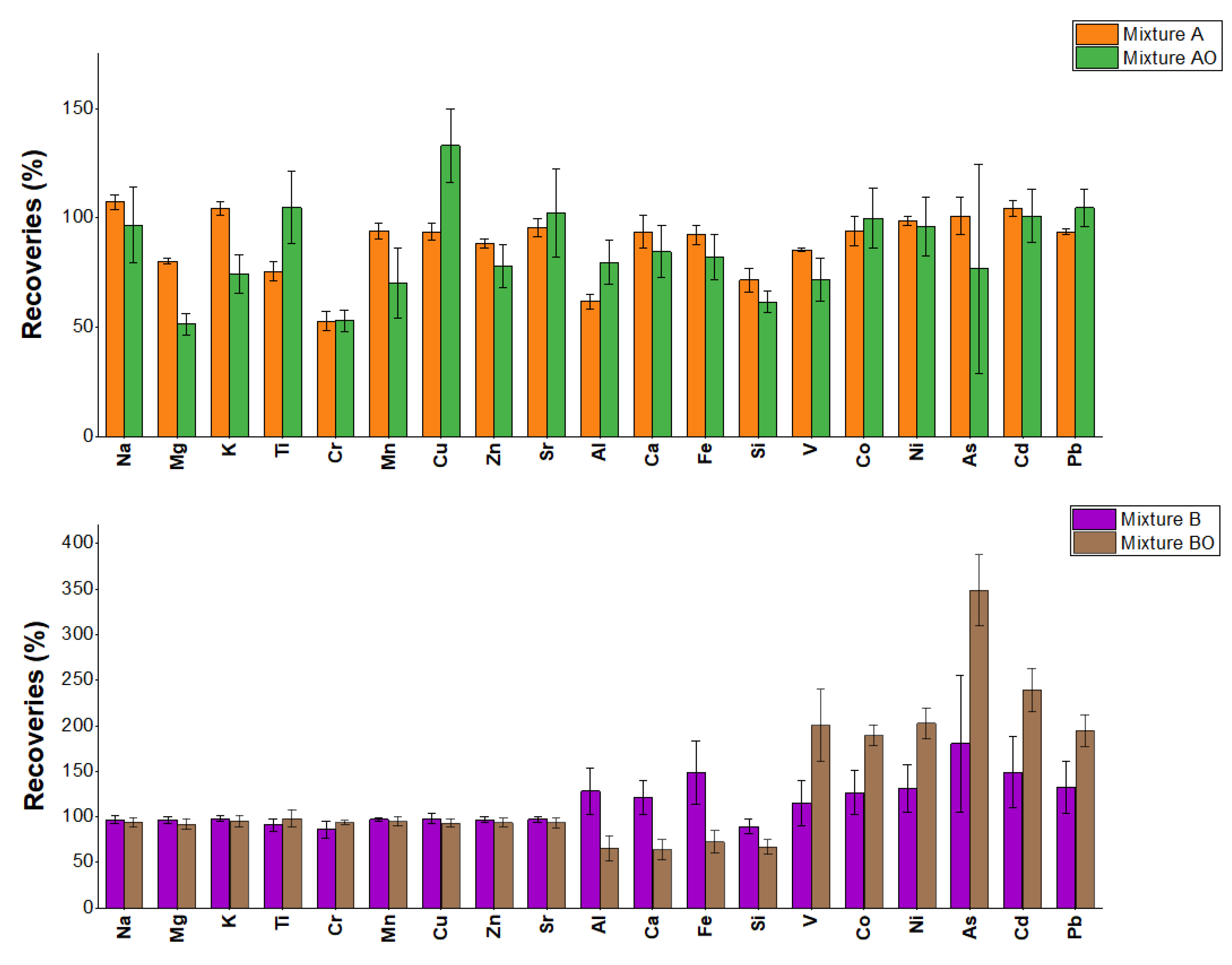
Figure 2.
Comparison between the percentages in mass obtained by the same tribological couple tested with EMFAB filter in dynamometer and tribometer set-up. Undetermined is the sum of the mass of the elements not determined (C, N, S, O mainly).
Figure 2.
Comparison between the percentages in mass obtained by the same tribological couple tested with EMFAB filter in dynamometer and tribometer set-up. Undetermined is the sum of the mass of the elements not determined (C, N, S, O mainly).
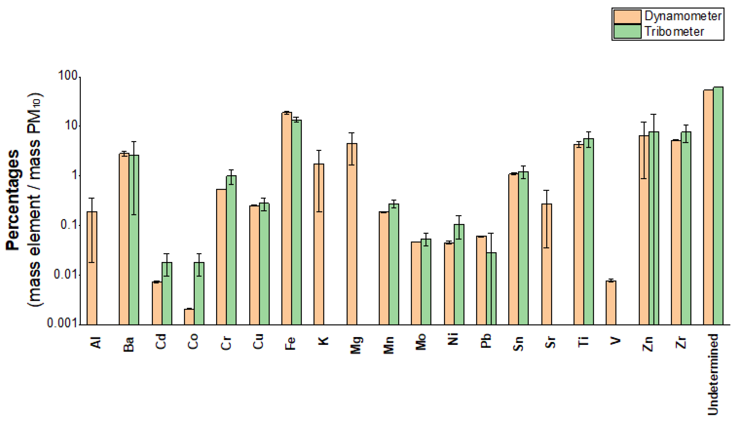
Figure 3.
SEM images of EMFAB filter (a,b) and PTFE filter (c,d) at 500 X and 5000 X of magnification with their EDS spectra on the right.
Figure 3.
SEM images of EMFAB filter (a,b) and PTFE filter (c,d) at 500 X and 5000 X of magnification with their EDS spectra on the right.

Figure 4.
Mean concentrations of the analytes in the blank EMFAB filters and in PTFE filters covered with tape (three replicates). Black bars indicate standard deviation. Sr, Zr and Si are below Limit of Detection (LOD) in PTFE filters covered with tape, whereas Cu and Pb are below LOD in EMFAB filters.
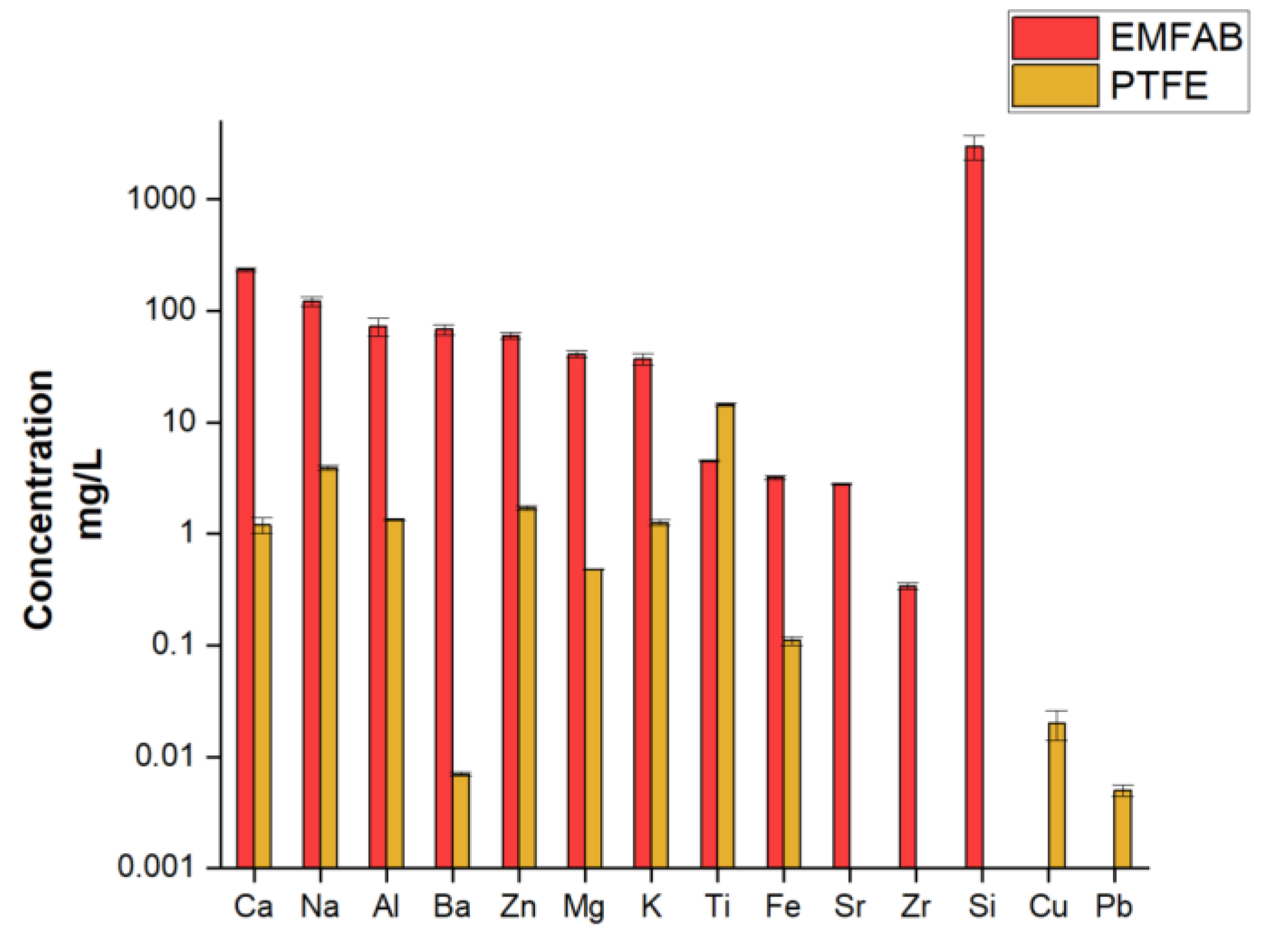
Figure 5.
A) PCA score plot of the twenty-three PM10 samples obtained by tribometer set-up. In green samples obtained with EMFAB filter (LET for LS material, NET for NAO materials), in violet samples obtained with PTFE filter (LTT for LS material, NTT-T/NTT-B for NAO materials). B) PCA loading plot of the twenty-three PM10 samples obtained by tribometer set-up. Concentration used for the dataset was mass of the element on mass of PM10.
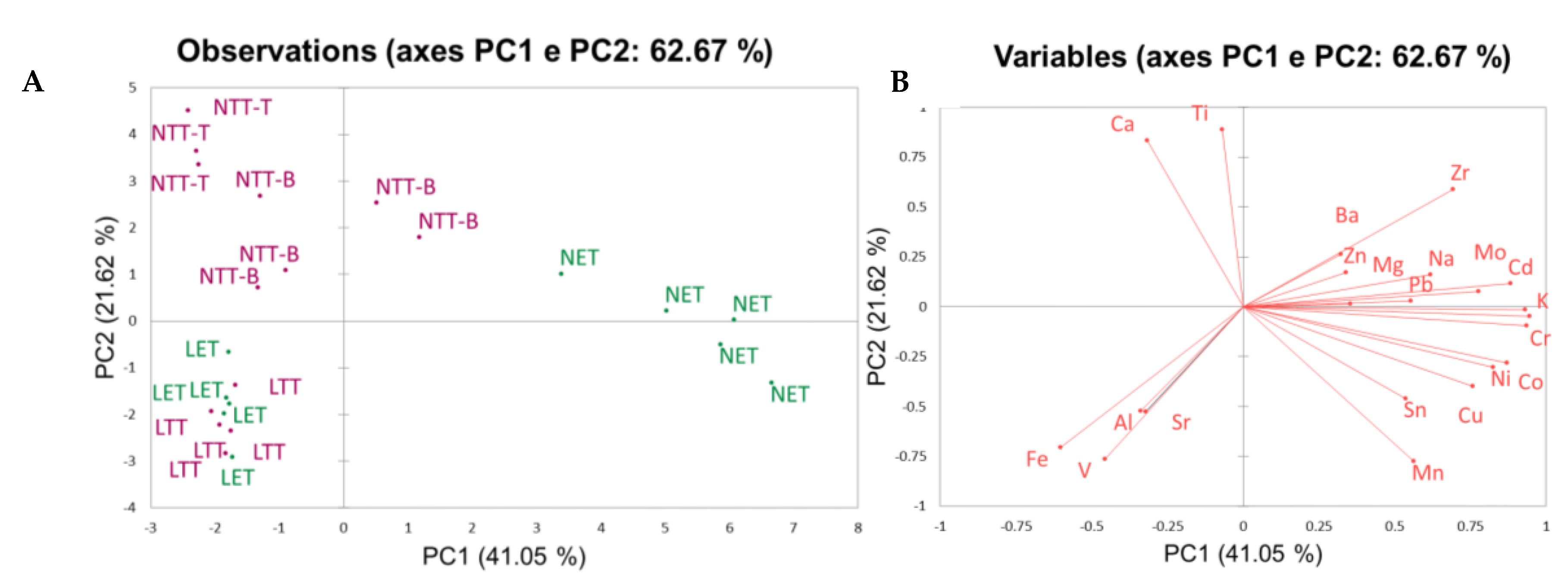
Figure 6.
Kruskal-Wallis p-values graphs for group 1 (LET vs LTT, top-left), group 2 (NET vs NTT-B/NTT-T, top-right), and group 3 (NTT-B vs NTT-T, bottom-middle).
Figure 6.
Kruskal-Wallis p-values graphs for group 1 (LET vs LTT, top-left), group 2 (NET vs NTT-B/NTT-T, top-right), and group 3 (NTT-B vs NTT-T, bottom-middle).
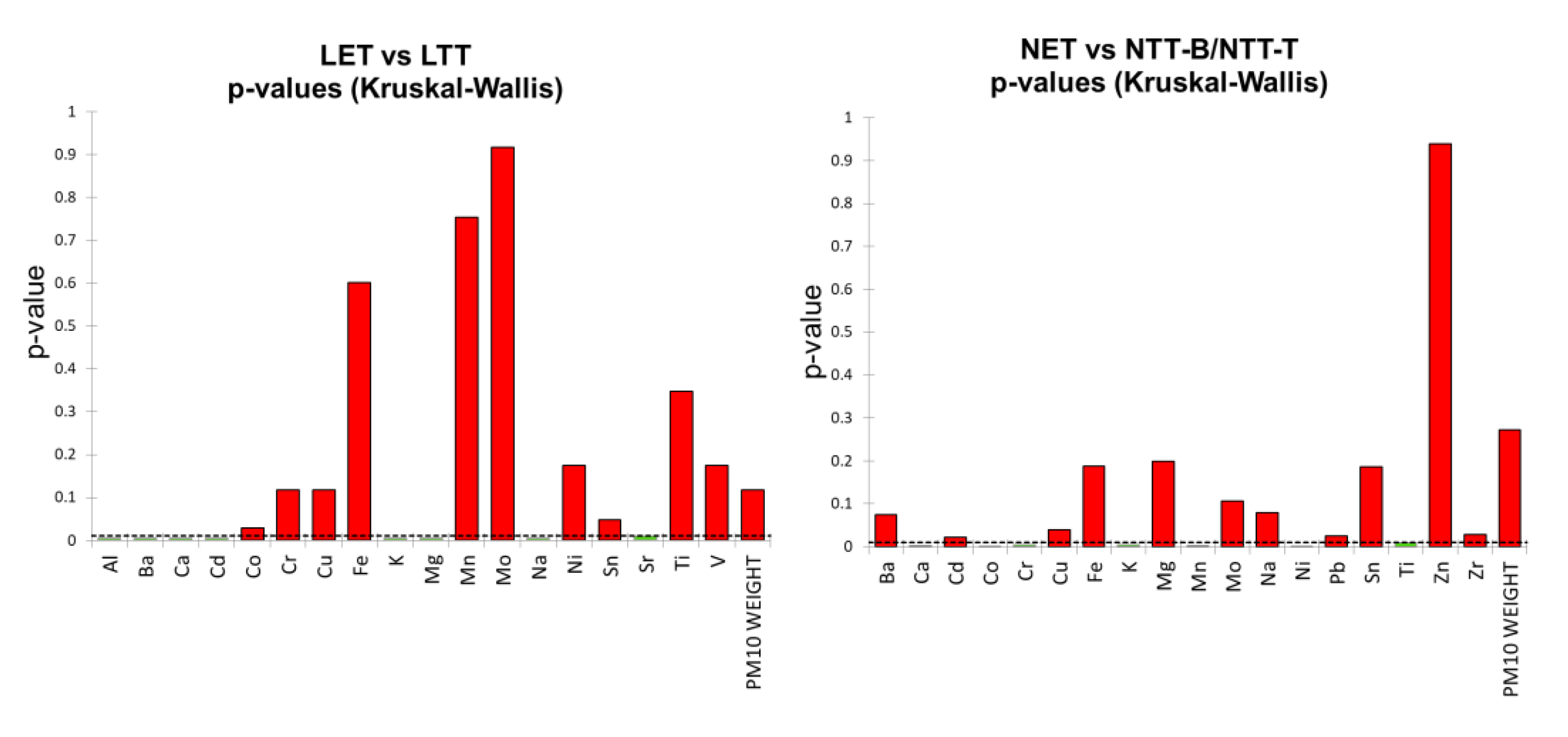
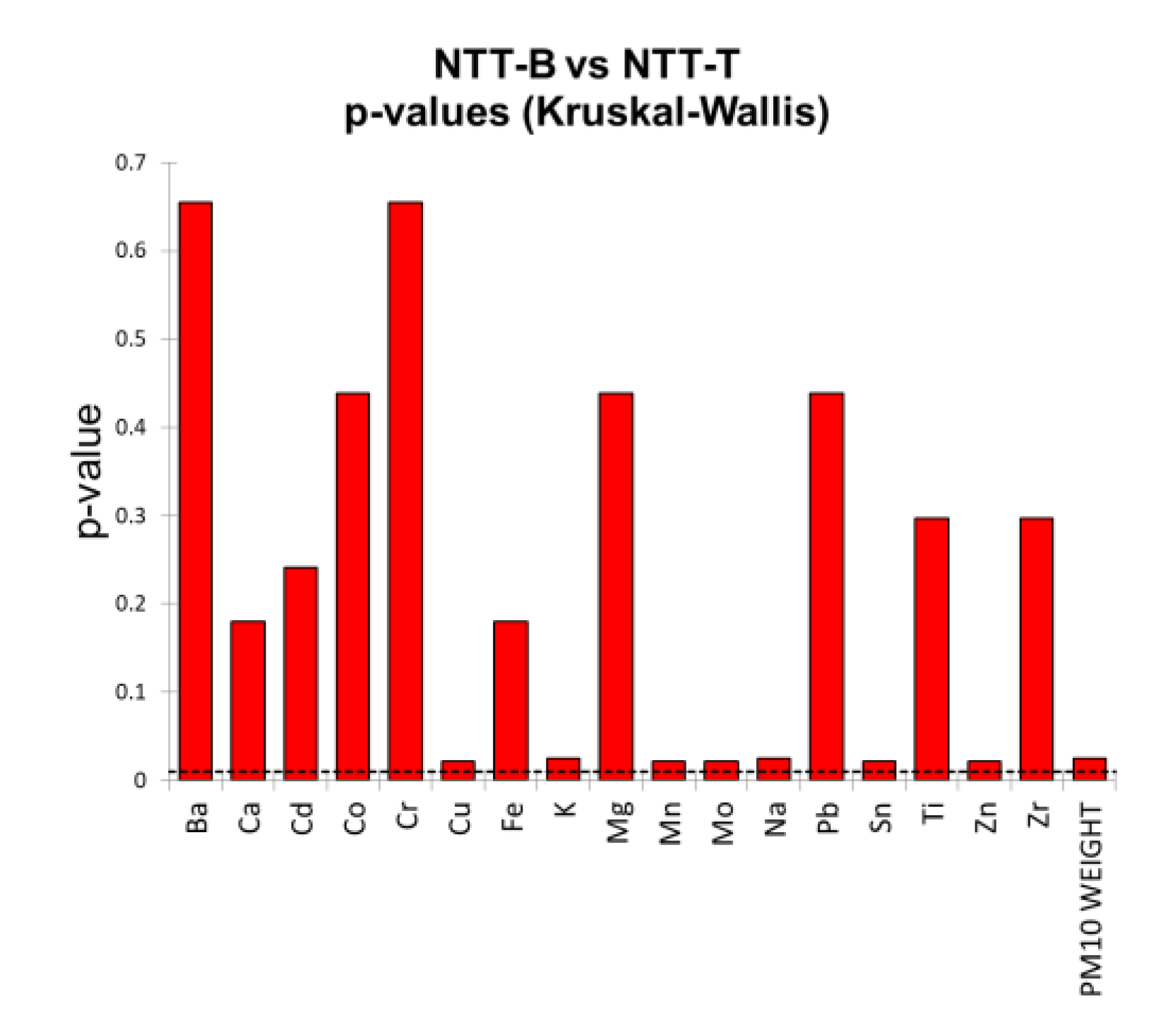
Figure 7.
PM10 samples analysed according to the different type of friction material and filter substrate.
Figure 7.
PM10 samples analysed according to the different type of friction material and filter substrate.
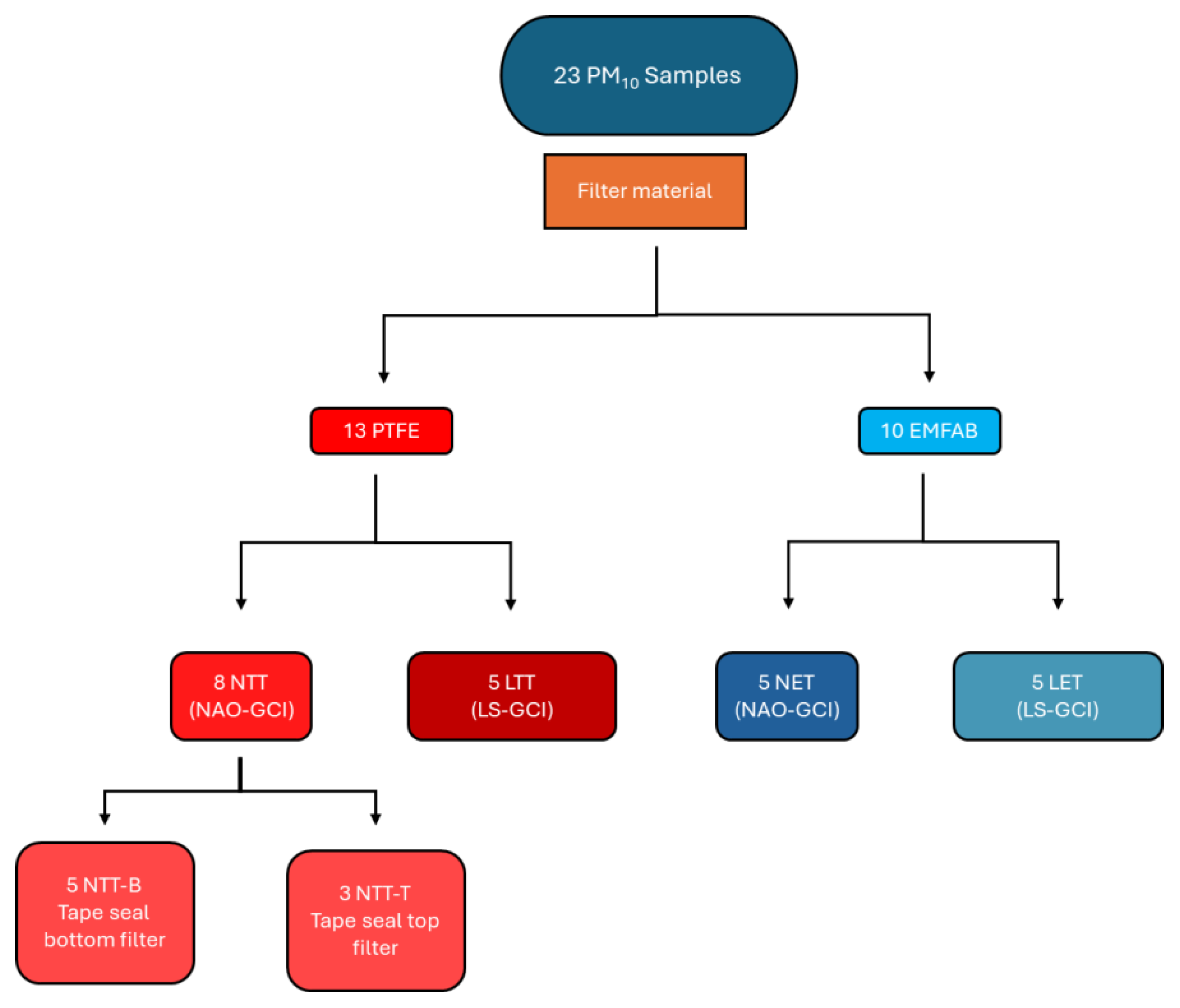
Figure 8.
Schematic representation of PM10 tribometer set-up used in this work.
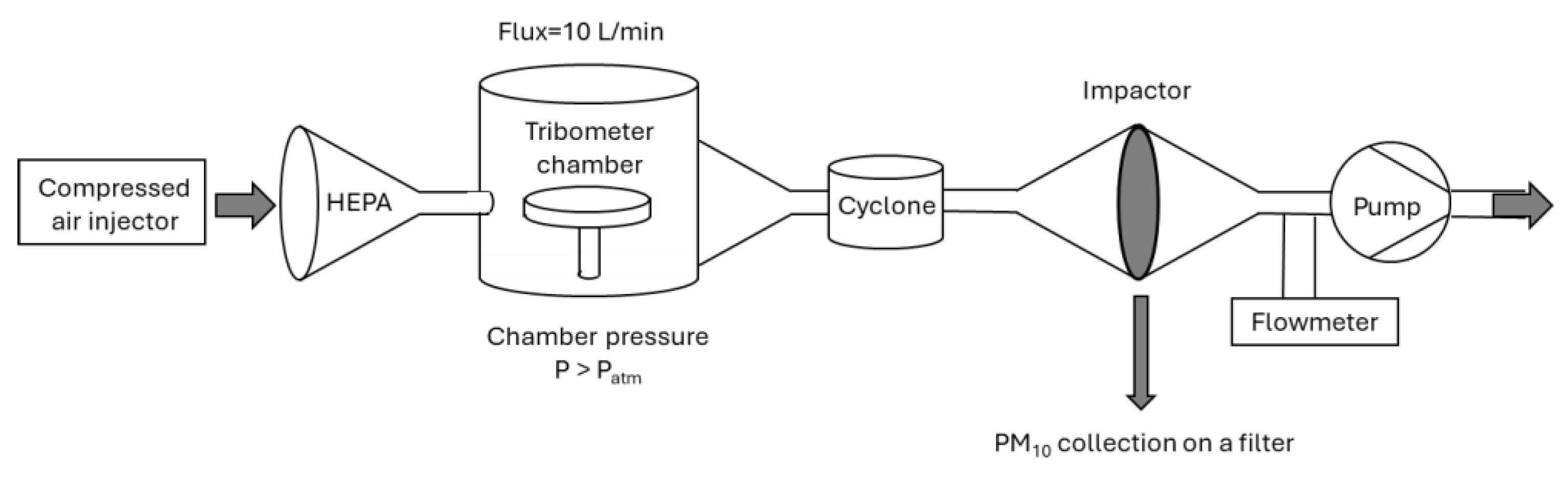
Figure 9.
Sample analysis workflow.
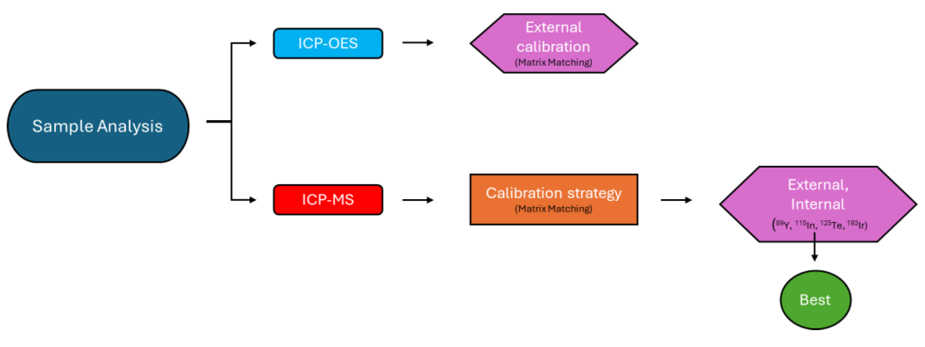

Table 1.
Mean recoveries and HORRATr values of the analytes determined in SRM NIST 1648a between mixture A, B and C. Values in bold indicate the acceptable values according to AOAC guidelines [45].
Table 1.
Mean recoveries and HORRATr values of the analytes determined in SRM NIST 1648a between mixture A, B and C. Values in bold indicate the acceptable values according to AOAC guidelines [45].
| Analyte | A mean recoveries (%) |
A HORRATr |
B mean recoveries (%) |
B HORRATr |
C mean recoveries (%) |
C HORRATr |
|---|---|---|---|---|---|---|
| Na | 107 | 1.0 | 97 | 1.4 | 44 | 8.0 |
| Mg | 80 | 0.8 | 97 | 1.9 | 77 | 1.0 |
| K | 104 | 1.4 | 98 | 1.8 | 47 | 10.6 |
| Ti | 76 | 1.9 | 91 | 2.5 | 19 | 3.6 |
| Cr | 53 | 2.1 | 86 | 2.8 | 33 | 4.3 |
| Mn | 94 | 1.2 | 97 | 0.6 | 92 | 0.5 |
| Cu | 94 | 1.4 | 98 | 1.8 | 93 | 1.2 |
| Zn | 88 | 0.8 | 97 | 1.1 | 91 | 1.8 |
| Sr | 96 | 1.1 | 97 | 0.8 | 72 | 0.5 |
| Al | 62 | 1.8 | 128 | 6.6 | 39 | 8.5 |
| Ca | 94 | 4.0 | 121 | 7.5 | 94 | 0.9 |
| Fe | 92 | 1.6 | 148 | 7.8 | 81 | 1.1 |
| Si | 72 | 3.8 | 89 | 4.6 | 1 | 64.0 |
| V | 85 | 0.2 | 115 | 3.6 | 76 | 1.5 |
| Co | 94 | 0.9 | 127 | 2.4 | 79 | 0.5 |
| Ni | 98 | 0.5 | 131 | 5.0 | 89 | 0.6 |
| As | 101 | 1.4 | 180 | 7.0 | 102 | 0.4 |
| Cd | 104 | 0.6 | 149 | 4.4 | 97 | 0.5 |
| Pb | 94 | 0.5 | 133 | 7.1 | 91 | 0.9 |
Table 2.
Mean percentage recoveries and HORRATr values of the elements analysed in BCR 176. Values in bold indicate the acceptable values according to AOAC guidelines [45].
Table 2.
Mean percentage recoveries and HORRATr values of the elements analysed in BCR 176. Values in bold indicate the acceptable values according to AOAC guidelines [45].
| Analyte | Mean recoveries (%) | HORRATr |
|---|---|---|
| Mn | 90 | 1.2 |
| Fe | 91 | 0.9 |
| Na | 101 | 1.5 |
| Zn | 88 | 1.1 |
| Ba | 94 | 0.9 |
| Cr | 78 | 1.2 |
| Cu | 103 | 0.5 |
| V | 109 | 0.6 |
| Ni | 104 | 1.5 |
| As | 97 | 1.9 |
| Pb | 103 | 1.0 |
Table 3.
Inter-sample and intra-sample RSD% values for the five types of samples analysed.
| Group | Intra-sample RSD% | Inter-sample RSD% |
|---|---|---|
| NET | 10 | 50 |
| NTT-B | 18 | 41 |
| NTT-T | 15 | 24 |
| LET | 8 | 22 |
| LTT | 7 | 20 |
Table 4.
Sample ID for the twenty-three samples analysed, with the indication of type of the filter, type of the friction material and PM10 weight obtained.
Table 4.
Sample ID for the twenty-three samples analysed, with the indication of type of the filter, type of the friction material and PM10 weight obtained.
| Sample ID | Type of friction material | Type of filter | PM10 weight |
|---|---|---|---|
| NTT-B 26 | NAO | PTFE | 0.46 |
| NTT-B 43 | NAO | PTFE | 0.57 |
| NTT-B 54 | NAO | PTFE | 0.80 |
| NTT-B 55 | NAO | PTFE | 0.28 |
| NTT-B 56 | NAO | PTFE | 0.44 |
| NTT-T 80 | NAO | PTFE | 0.16 |
| NTT-T 81 | NAO | PTFE | 0.15 |
| NTT-T 82 | NAO | PTFE | 0.14 |
| NET 14 | NAO | EMFAB | 0.56 |
| NET 16 | NAO | EMFAB | 0.56 |
| NET 41 | NAO | EMFAB | 0.47 |
| NET 47 | NAO | EMFAB | 0.23 |
| NET 42 | NAO | EMFAB | 0.44 |
| LTT 28 | LS | PTFE | 7.09 |
| LTT 37 | LS | PTFE | 12.52 |
| LTT 38 | LS | PTFE | 7.47 |
| LTT 40 | LS | PTFE | 13.93 |
| LTT 49 | LS | PTFE | 8.05 |
| LET 17 | LS | EMFAB | 17.34 |
| LET 33 | LS | EMFAB | 8.96 |
| LET 34 | LS | EMFAB | 10.64 |
| LET 35 | LS | EMFAB | 13.26 |
| LET 36 | LS | EMFAB | 16.34 |
Disclaimer/Publisher’s Note: The statements, opinions and data contained in all publications are solely those of the individual author(s) and contributor(s) and not of MDPI and/or the editor(s). MDPI and/or the editor(s) disclaim responsibility for any injury to people or property resulting from any ideas, methods, instructions or products referred to in the content. |
© 2025 by the authors. Licensee MDPI, Basel, Switzerland. This article is an open access article distributed under the terms and conditions of the Creative Commons Attribution (CC BY) license (http://creativecommons.org/licenses/by/4.0/).
Copyright: This open access article is published under a Creative Commons CC BY 4.0 license, which permit the free download, distribution, and reuse, provided that the author and preprint are cited in any reuse.


