Submitted:
17 November 2025
Posted:
18 November 2025
You are already at the latest version
Abstract
Geostrophic current velocity anomalies at the mid-latitudes of the three oceans are highlighted, and their role in the genesis of low-pressure systems in boreal/austral winter. These anomalies are attributed to quasi-stationary Rossby waves resonantly forced by the solar declination in harmonic modes. They develop along the western boundary currents as they leave the continents to re-enter the five subtropical gyres. In the North and South Atlantic, the thermocline behaves as a resonant cavity with rigid boundaries at the edges of the western boundary currents, i.e. the Gulf Stream and the Brazil Current, traversed by first-baroclinic mode, first-meridional mode Rossby waves. In the Indian Ocean, the retroflection of the Agulhas Current south of the African continent causes resonance in two different ways west and east of the Cape of Good Hope: resonance of second-baroclinic mode Rossby waves in the first case, and first-baroclinic mode Rossby waves in the second. The resonant forcing of second-baroclinic mode Rossby waves is also observed in the East Australian Current as it flows along Australia. In the North Pacific, resonant forcing of first-baroclinic mode Rossby waves is observed along the Kuroshio, off the east coast of Japan. Geostrophic current velocity anomalies are proving to be convective zones with a significant climatic impact. Within relevant period ranges, this is highlighted by the close coherence of 1 in the geopotential height anomalies at 500 hPa revealing a causal relationship between the geostrophic current velocity anomalies and the formation of low-pressure systems. The objective of this study is to identify the phenomena that precede the formation of winter low-pressure systems at mid-latitudes. The precursor signals observed in convective zones could be relevant candidates for anticipating these meteorological phenomena 10 to 15 days in advance using deep learning techniques.
Keywords:
Rossby waves
; resonant forcing
; mid-latitudes
; low-pressure systems
1. Introduction
1.1. The State of the Art
The increase in extreme events, heat waves and rainfall, over the past few decades has sparked curiosity to elucidate the underlying phenomena. Several extreme phenomena that have occurred recently during the northern hemisphere summer have been linked to patterns of persistent high-amplitude waves, whether heat waves in Russia, Europe or the United States, or floods in Pakistan and Europe [1]. Rapid Arctic warming is suspected to be the cause of the persistence of damaging weather events in the northern hemisphere, i.e. drought, heat waves, prolonged cold spells and storminess, but more particularly in North America, Europe and western Asia [2]. It has been shown that the frequency of planetary wave resonance events has tripled over the last half-century, leading to changes in underlying climatic conditions that favor these events, including the amplification of Arctic warming and land-sea thermal contrast [3]. A prolonged pattern of resonant planetary waves, prior to the "heat dome" episode that occurred in the Pacific Northwest in June 2021, created a soil moisture deficit that amplified the warming of the lower atmosphere through strong nonlinear soil moisture feedbacks, thus favoring this unprecedented heat episode [4].
In this context, there is increasing interest in quasi-resonance phenomena to explain the sudden development of extreme phenomena. It appears that such phenomena, which are intrinsically linked to the properties of the atmosphere and oceans, as well as to the forcing mode attributed to the declination of the sun or to orbital cycles, are taking on increasing importance under the influence of global warming. The link between recurrence of transient Rossby wave packets, blocks, and quasi-resonant amplification in the Southern Hemisphere was investigated [5]. The relationship between remarkable heatwaves during summer 2018 and quasi-resonant amplification mechanism, combining a double jet presence with quasi-stationary and highly-amplified Rossby wave as a response has been highlighted [6].
1.2. The Ubiquity of Rossby Waves
The resonance of oceanic and atmospheric Rossby waves proves crucial in explaining both the variety of climate in the short, medium and long term, as well as extreme weather events. Regarding oceanic Rossby waves, they reflect the oscillation of the pycnocline, which generally coincides with the thermocline. They are found in the tropics as well as in the mid-latitudes along subtropical gyres. As for atmospheric Rossby waves, they are found at the tropopause at the interface between the polar jet and the ascending air column at the meeting of the polar and Ferrel cell circulation or between the subtropical jet and the descending air column at the meeting of the Ferrel and Hadley cell circulation.
The period of Rossby waves varies considerably, from a few days to a year for atmospheric waves, from a few days to several million years for oceanic waves. The spectrum of periods depends on the basin boundaries (these boundaries disappear for oceanic waves propagating around subtropical gyres or for atmospheric waves propagating around the earth), latitude, and the mean eastward-propagating flow into which westward-propagating Rossby waves are embedded, so that they appear to propagate eastward. However, the large amplitude of this spectrum explains why Rossby waves are frequently forced into resonance. Since these baroclinic waves can be forced by variations in solar irradiance, they have a propensity to tune their natural period to the forcing period of solar and orbital cycles, whether seasonal, annual, or multi-year. For this to happen, it is sufficient that the forcing period is found in the spectrum of natural periods of Rossby waves.
Linearizing the equations of motion of forced Rossby waves shows that they are characterized by their amplitude as well as by their modulated zonal and meridional current velocities, which are proportional to the amplitude [7]. The coupling of Rossby waves results from geostrophic forces acting on the scale of the basin. When geostrophic balance is perturbed under the influence of these forced waves, it naturally tends to re-establish itself. This restoring force acting on each of the quasi-stationary waves can be interpreted by considering these Rossby waves as coupled inertial oscillators governed by the Caldirola–Kanai (CK) equations [8,9]. In exchange zones subjected to the geostrophic forces of the basin, the restoring force of these coupled oscillators taken two by two is proportional to their difference in zonal current velocity. Indeed, geostrophic balance is not altered when velocities are equal, whereas it is altered all the more when velocities differ. In this case, the restoration of geostrophic balance implies that the fastest current slows down, and the slowest current accelerates in the exchange zone.
The general formulation of the behavior of forced and coupled quasi-stationary Rossby waves by assimilating them to forced inertial CK oscillators, the damping parameter of which refers to the Rayleigh friction, allows such dynamic systems to be endowed with equally general properties. First, these Rossby waves are forced resonantly. This stems from the fact that their apparent wavelength adapts so that the wave's natural period remains close to the forcing period when the latter varies. Note that Rossby waves with long wavelengths are approximately non-dispersive, and their apparent wavelength is proportional to the period. Secondly, these Rossby waves are forced into harmonic and/or subharmonic modes. Since the period of the fundamental wave coincides with the forcing period, harmonics and subharmonics occur, the periods of which are multiples or divisors of the fundamental wave's period. This condition is necessary to ensure the stability of the dynamic system formed by the superposition of coupled multifrequency quasi-stationary Rossby waves. When these conditions are met, each oscillator receives, on average, as much energy from the other oscillators as it releases.
1.3. The Climatic Impact of Quasi-Stationnary Rossby Waves
The climatic impact of resonantly forced quasi-stationary Rossby waves is due to the fact that the zonal and meridional currents of the fundamental wave, which are in quadrature, are warm or cold depending on their direction of propagation. This results from the baroclinicity of Rossby waves and their resonant forcing by variations in solar irradiance. Each harmonic or subharmonic inherits this property which is directly related to the oscillation of the wave. For oceanic waves, this results from the oscillation of the thermocline which generates modulated zonal and meridional currents. For atmospheric waves, it is the variations in height of the interface at the tropopause of polar or subtropical waves that are involved. These interfaces move up-and-down depending on whether the column of air supporting them is warm or cold (polar and subtropical waves are in opposite phase), which generates modulated zonal and meridional airflows.
2. Materials and Method
2.1. Data
The geopotential height as a function of atmospheric pressure (17 levels), (2.5°×2.5°) is provided by the National Oceanic and Atmospheric Administration (NOAA) PSL, Boulder, CO, USA. The daily gridded data from 1979 to now [10] are available at https://www.psl.noaa.gov/data/gridded/data.ncep.reanalysis2.html, accessed on 13 May 2024.
Daily (1/4°×1/4°) Sea Surface Temperature (SST) data are provided by the NOAA [11,12,13,14]. The data are averaged on grids (1°×1°) to obtain a resolution adapted to the needs of the present study.
Daily gridded data (1/4°×1/4°) of the geostrophic current velocity are provided by the NOAA [15].
2.2. Wavelet Analysis
A Morlet cross-wavelet analysis is performed to estimate the amplitude, i.e. the square root of the wavelet power, of variations in characteristic period bands of three state variables, that is, geostrophic current velocity, SST, and geopotential height. Their coherence and phase are expressed in relation to a reference time series [16]. In the case of the geostrophic current, the reference is located in an anomaly to the west of the basin. Thus, coherence and phase highlight the unity of anomalies at the basin scale, with high coherence indicating a common cause, and phase indicating the time lag relative to the reference (which only makes sense where coherence is high). In the case of the SST and the geopotential height at 500 hPa, the reference is the SST located near the previous reference. The SST reference is thus considered as an indicator of the convective processes that occur at the location of the geostrophic current velocity anomalies. In this way, this highlights the unity of the SST at the basin scale, but also a causal relationship between the geostrophic current velocity anomaly and the geopotential height anomalies.
3. Results
3.1. Observation of Oceanic Rossby Waves at Mid-Latitudes
In Figure 1, the amplitude, coherence, and phase of the geostrophic current velocity in the North Atlantic are represented on 01/01/2005 for 1/24-, 1/12-, 1/6-, and 1/3-year period harmonics, the fundamental annual wave, and the 8-year period subharmonic. The fundamental wave is distinguished by the fact that its period coincides with that of the forcing, which results from the declination of the sun.
As shown from the phase, the waves have increasing wavelengths, characterizing a series of oscillations and highly coherent structures, which suggests that they are Rossby waves forced by the declination of the sun. Indeed, coherence of the geostrophic current velocity is ubiquitous in all period ranges (Figure 1b, e, h, k, n). But the amplitude increases considerably where the western boundary current, i.e. the Gulf Stream, flows away from the American continent to re-enter the North Atlantic gyre (Figure 1 a,d,g,j,m). The increase in wave amplitude along the gyre suggests that the thermocline is well-defined there, differentiating the cold deep waters from the warm floating waters of tropical origin. The westward phase velocity of Rossby waves is less than the eastward velocity of the mean western boundary current in which they are embedded so that they appear to travel eastward. Along the western boundary current, the phase shows that these Rossby waves are coherent and in opposite phase regardless of the period range, which highlights the local geostrophic balance (Figure 1c,f,i,l,o). These observations confirm a posteriori the presence of a fundamental wave resonantly forced by the variation in annual insolation attributed to the sun's declination, which produces a whole range of harmonics and subharmonics.
As shown in the Figure 1p,q,r, the exchange zones have a small surface area. They are omnipresent throughout the North Atlantic. Coupling between Rossby waves of different periods occurs mainly for harmonics close to the fundamental wave, as well as for harmonics between them. Indeed, the density of the exchange zones is higher for the harmonic pairs of periods (Figure 1q) and (Figure 1r) than for (Figure 1p).
3.2. Acceleration of the Modulated Geostrophic Current
Figure 1d, g shows that the velocities of geostrophic currents along the crests of 1/6- and 1/3-year period harmonics are higher than those of the fundamental wave in Figure 1j. According to observations made in the three oceans at mid-latitudes, the maximum velocity reached by geostrophic currents where the western boundary currents leave their respective continents to re-enter the subtropical gyre is shown in Figure 2 for the different harmonics. Figure 2a suggests that the North Atlantic basin behaves like a resonator with a bandwidth whose periods are between 1/48 year and 1 year. For the 1/6 year period, the maximum amplitude of the modulated geostrophic current velocity is nearly double that of the fundamental wave.
According to Figure 3a, d the peak maximum is centered approximately at 37°N, 60°W for both selected dates, i.e. 01/07/2004 and 01/01/2005. The presence of such a zone where the geostrophic current is subject to strong acceleration is found in all three oceans after the western boundary current leaves the continent, always in the same location, in all seasons. This acceleration appears to result from an adequacy between the length of the Rossby waves and the width of the western boundary current.
3.2.1. The North Atlantic
In the North Atlantic, Figure 3b, e shows that the spatial coherence of Rossby waves extends latitudinally, which suggests that a resonance occurs transverse to the direction of traveling whatever the season, summer or winter. The thermocline behaves like a resonant cavity with rigid boundaries at the edges of the western boundary current, crossed by first-baroclinic mode, first-meridional mode Rossby waves. This assertion is suggested by the coherence of the Rossby waves both inside and outside the resonance zone. This reflects the oscillation of the main thermocline, with a single longitudinal crest.
From the equations of motion, the velocity of the meridional modulated currents is proportional and in quadrature with the oscillation of the thermocline. When these meridional currents are synchronized, they reach their maximum at the same time, traveling northward or southward depending on the phase of the Rossby wave. The acceleration in the resonance zone followed by a deceleration of the meridional current between the two edges of the western boundary current appears to be the cause of the increase in the amplitude of the thermocline oscillation, which is self-sustaining. Indeed, the increase in the amplitude of oscillation of the thermocline proportionally leads to an increase in the velocity of the meridional geostrophic current. The 1/6-year period seems to be the most conducive to this resonance phenomenon.
3.2.2. The South Atlantic
Figure 4b shows a similar behavior for the Brazil Current in the South Atlantic although the resonance curve exhibits a plateau between the 1/24 and 1/3 year periods (Figure 2b). The Brazil Current coming from the north meets the Malvinas Current coming from the south and moves away from the South American continent at latitude 40°S (Figure 4). Here again we observe a latitudinal extension of the coherence where the velocity of the geostrophic current is maximum, close to the maximum of the resonance curve, whatever the season (Figure 4b,e).
3.2.3. The Indian Ocean
Regarding the Indian Ocean, the resonance curve is strongly asymmetrical (Figure 2c). The retroflection of the Agulhas Current south of the African continent causes the resonance to occur in two different ways west and east of the Cape of Good Hope (Figure 5). It occurs in the absence of coherence in the first case, and in a highly coherent way in the second, with a strong latitudinal extension of the geostrophic current velocity anomaly. The anomaly occurring downstream of the retroflection of the Agulhas Current is reminiscent of what has been observed in the North and South Atlantic, i.e. a synchronous resonance at the basin scale. On the other hand, the asynchronous resonance where the retroflection occurs suggests that it is the second-baroclinic mode that is resonantly forced and no longer the first-baroclinic mode.
3.2.4. The South Pacific
This asynchronous resonance is also observed in the Eastern Australian Current as it flows along Australia (Figure 6). The coherence of the anomalies is low (Figure 6b,e). The resonance curve increases monotonically up to the 1/3-year period harmonic (Figure 2e), highlighting the persistence of anomalies whatever the season (Figure 6a,d). Again, this highlights the resonant forcing of the second-baroclinic mode Rossby waves, which is corroborated by their long period.
3.2.5. The North Pacific
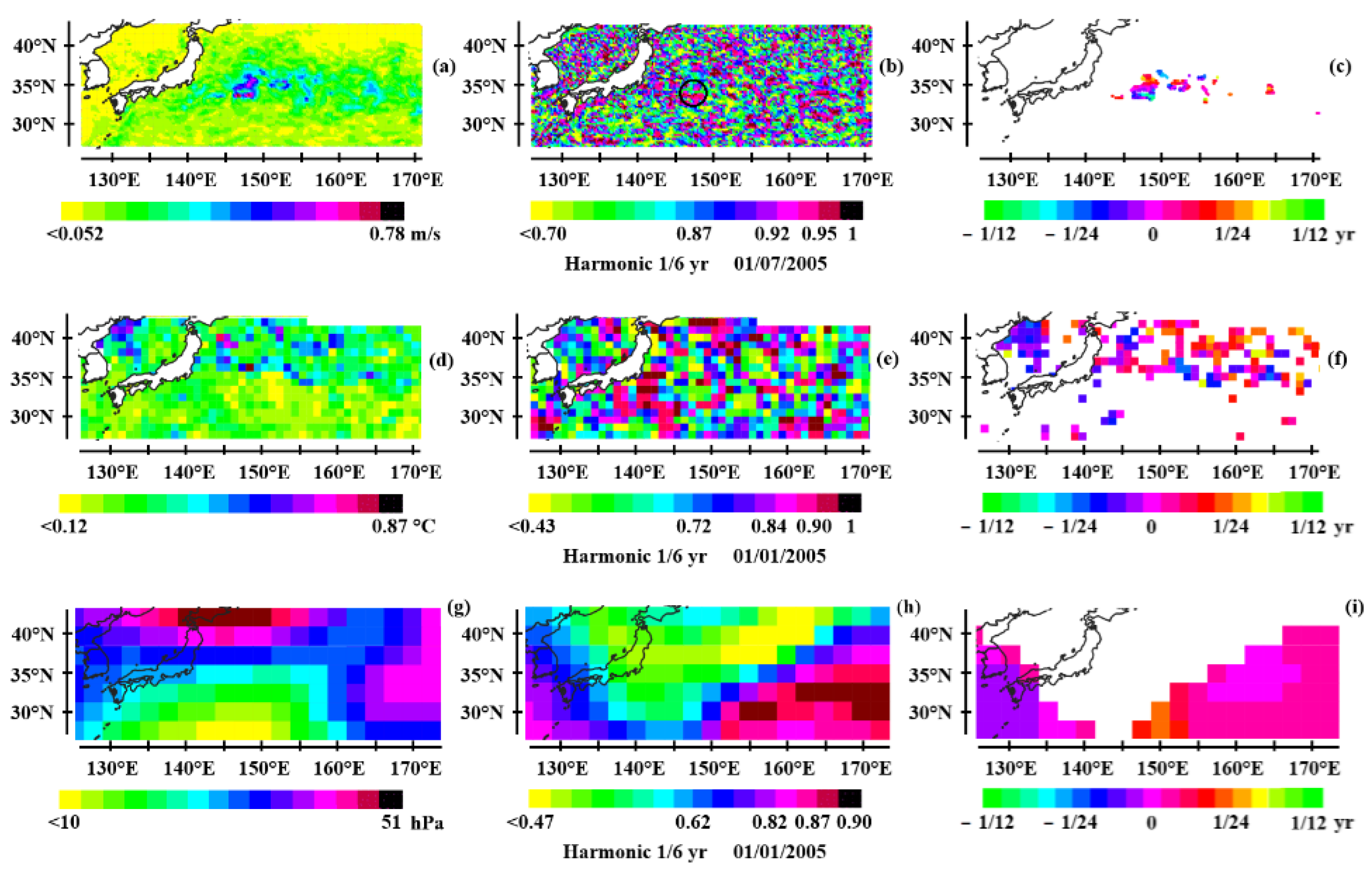
In the North Pacific the resonance is synchronous at the basin scale, in particular along the Kuroshio off the Eastern Japan coast (Figure 7). The resonance curve highlights a weak acceleration of the 1/6-year period harmonic (Figure 2d) whose geostrophic current velocity reaches 0.78 m/s on 01/07/2005: Figure 7a. The weakness of the effective feedback mechanism could be due to the width of the Kuroshio current being greater than the wavelength of the Rossby waves when it merges with the Oyashio Current to form the North Pacific Current (Figure 7a,d).
3.3. Impact on Climate
The mosaic of Rossby waves in the mid-latitudes promotes ocean-atmosphere interactions, especially where these waves exhibit large amplitudes. These exchanges are exacerbated by the coexistence of modulated geostrophic currents flowing westward and eastward, as occurs in the convective zones. These currents are warm or cold depending on whether they flow westward or eastward. Resulting from harmonic oscillations of the fundamental annual wave, which is resonantly forced from the solar declination, this property is inherited from the fundamental wave itself. At mid-latitudes, the associated modulated zonal current warms during the summer boreal/austral season and cools during the winter boreal/austral season, while its direction of propagation reverses. This property remains valid for each of the harmonics. This reflects the intra-seasonal variations in the shoaling and deepening of the thermocline, which are synchronized with the modulated zonal and meridional currents.
The modulated currents being cold or warm depending on their traveling direction, their assembly along the western boundary current forms a mosaic that favors baroclinic instabilities in the atmosphere. This is where most low-pressure systems originate in the mid-latitudes. Indeed, for a cold environmental adiabat, convective available potential energy (CAPE) increases above an increasing SST. So moist convection is promoted, which transiently lifts the level from which the outgoing longwave radiation (OLR) escapes to the space [17]. The atmosphere is even more perturbated as the increase in CAPE is significant.
3.3.1. Sea Surface Temperature
Convective zones characterized by a strong acceleration of geostrophic currents resulting from first- and second-baroclinic mode, first-meridional mode Rossby waves resonantly forced by solar declination produce SST anomalies, the most significant of which are shown in Figure 3g, h, i for the North Atlantic, Figure 4g, h, i for the South Atlantic, Figure 5d, e, f for the Indian Ocean, Figure 6g, h, i for the South pacific, and Figure 7d, e, f for the North Pacific. They occur in winter, reflecting the western boundary current with a more or less significant spatial offset. This discrepancy indicates that ocean-atmosphere interactions are playing a role in producing sea surface temperature anomalies: baroclinic instabilities in the atmosphere favor convective processes. Warm, moisture-laden air exchanges sensible and latent heat with the ocean after being advected. In the South Atlantic, the anomaly splits into two branches.
The coherence of SST anomalies shows maxima that are fairly uniformly distributed across the study area, outside the zone of influence of the continents. With the exception of the South Pacific, the spatial extent of the anomaly's amplitude occurs independently of coherence. It is the western boundary current that is decisive.
The phase represented where the SST anomalies are most significant (first quartile) may be relatively uniform or reflect the advection process as this occurs in the North Atlantic (Figure 3i). In this case, the SST anomaly develops around latitude 40°N off the east coast of North America. Initially in phase with or slightly ahead of the reference, the anomaly extends eastward after 15 days (1/24 of a year). Elsewhere, the anomaly is practically in phase with the reference. These observations suggest that the SST anomaly is initiated in the convective zone west of the basin then extends eastward through ocean/atmosphere coupling along the western boundary current while also being advected.
3.3.2. Geopotential Height at 500 hPa
Geopotential height at 500 hPa is used to highlight the atmospheric response to the evolution of the convective processes in the west of the basin. In order to establish a causal relationship between the convective processes and the geopotential height anomalies, a common reference is used, the SST in the convective zone. The only geopotential height anomalies considered significant are those for which the coherence is high. A geopotential height anomaly is usually strongly out of phase, which indicates that a positive SST anomaly generates a low-pressure system (i.e. a negative geopotential height anomaly), conducive to the development of a cyclonic system. In order to make the phase as significant as possible to represent the evolution of the barometric anomaly, the geopotential height at 500 hPa is time-averaged over a 2-month segment centered on the date of the observation.
Although the atmospheric response to a positive SST anomaly exhibits some variability, certain patterns occur frequently, providing insight into the potential meteorological impact of the convective zone. In the North Atlantic, the low-pressure system originates where the coherence of the geopotential height is the highest off the southeastern coast of the United States around latitude 35°N (Figure 3k). Then barometric low is deepening, as revealed by its amplitude (Figure 3j), while moving northward to around latitude 40°N after about ten days (Figure 3l). In the South Atlantic, the low-pressure system originates in southeastern Brazil and off its southeastern coast around latitude 30°S (Figure 4k) and then strengthens while moving southward to latitudes 35°S-40°S (Figure 4j) after about fifteen days (Figure 4l). In the Indian Ocean, the low-pressure system originates off the southern coast of Africa around latitude 30°S (Figure 5h) and then strengthens while moving southeastward to latitudes 35°S-40°S (Figure 5g) concomitantly (Figure 5i). It should be noted that the anomaly located off the coast of South Africa to the west is not part of the low-pressure system being studied because its coherence is very weak. In the South Pacific, the low-pressure system originates off the southeastern coast of Australia between latitudes 40 and 60°S (Figure 7k), and develops nearly in that latitudes while shifting westward almost simultaneously (Figure 7j,l). In the North Pacific, the low-pressure system originates off the eastern coast of Japan around latitude 30-35°N, beyond longitude 150°E (Figure 7h), and develops in that location almost simultaneously (Figure 7g,i). Here again, the anomaly located off the northern coast of Japan (Figure 7g) is not part of the low-pressure system being studied because its coherence is very weak.
These observations highlight the driving role of the convective zone in the genesis of low-pressure systems in winter, which is evidenced by the high coherence of the induced barometric anomaly. This applies regardless of the period of the harmonic, whatever the baroclinic mode of Rossby waves. The delay required for the initiation of the barometric anomaly is deduced from the phase where the coherence is maximal. Since the reference and the geopotential height vary inversely, a phase equal to zero indicates that the barometric trough is initiated with a half-period delay. This is what occurs in the Indian Ocean (Figure 5i) as well as the North Pacific (Figure 7i). In the North (Figure 3l) and South Atlantic (Figure 4l), as well as in the South Pacific (Figure 7l), the phase is in quadrature, which means that the delay is approximately one quarter of a period.
4. Conclusions
At mid-latitudes, Rossby waves resonantly forced by the solar declination in harmonic mode develop where the thermocline is well differentiated, i.e., along the western boundary currents as they leave the continents to re-enter the five subtropical gyres. Geostrophic current velocity anomalies result from resonant forcing of first- or second-baroclinic mode Rossby waves. The range of resonance periods is wide, stretching between 1/12- to 1/3-year. These anomalies play a key role in the formation of low-pressure systems.
- In the North and South Atlantic, the thermocline behaves as a resonant cavity with rigid boundaries at the edges of the western boundary currents, i.e. the Gulf Stream and the Brazil Current, traversed by first-baroclinic mode, first-meridional mode Rossby waves.
- In the Indian Ocean, the retroflection of the Agulhas Current south of the African continent causes resonance in two different ways west and east of the Cape of Good Hope: resonance of second-baroclinic mode Rossby waves in the first case, and first-baroclinic mode Rossby waves in the second.
- The resonant forcing of second-baroclinic mode Rossby waves is also observed in the East Australian Current as it flows along Australia. In the North Pacific, resonant forcing of first-baroclinic mode Rossby waves is observed along the Kuroshio, off the east coast of Japan.
These six convective zones are conducive to the formation of low-pressure systems. Causal relationships are established between sea surface temperature anomalies, indicative of convective zones, and the initiation and maturation of low-pressure systems. Thus, warm, moisture-laden air exchanges sensible and latent heat with the ocean after being advected. Widespread SST anomalies develop nearly one eighth of a period later. Convective processes can potentially lead to the formation of a synoptic-scale cyclonic systems [18]. Despite the significant variability to which this sequence of events is subject, the most frequent patterns are represented, from the formation of the SST anomaly in the convective zone to the formation of the geopotential height anomaly. There is a time lag of between a quarter and half a period between these two events.
The objective of this study was to identify the phenomena that anticipate the formation of boreal/austral winter low-pressure systems at mid-latitudes. The precursor signals observed in convective zones could be used to anticipate these weather events using deep learning techniques. This should lead to a significant breakthrough in the prediction of these weather events.
Funding
This research received no external funding.
Institutional Review Board Statement
Not applicable.
Informed Consent Statement
Not applicable.
Data Availability Statement
The original contributions presented in this study are included in the article. Further inquiries can be directed to the corresponding author.
Acknowledgments
We thank the editor and the reviewers for their helpful comments.
Conflicts of Interest
The author declares no conflicts of interest.
References
- Kornhuber, K.; Petoukhov, V.; Petri, S.; Rahmstorf, S.; Coumou, D. Evidence for wave resonance as a key mechanism for generating high-amplitude quasi-stationary waves in boreal summer. Climate Dynamics 2017, 49, 1961–1979. [Google Scholar] [CrossRef]
- Francis, J.A.; Skific, N.; Vavrus, S.J. North American weather regimes are becoming more persistent: Is Arctic amplification a factor? Geophysical Research Letters 2018, 45, 11414–11422. [Google Scholar] [CrossRef]
- Li, X.; Mann, M.E.; Wehner, M.F.; Christiansen, S. Increased frequency of planetary wave resonance events over the past half-century. Proc. Natl. Acad. Sci. USA 2025, 122, e2504482122. [Google Scholar] [CrossRef] [PubMed]
- Li, X.; Mann, M.E.; Wehner, M.F.; Rahmstorf, S.; Petri, S.; Christiansen, S.; Carrillo, J. Role of atmospheric resonance and land–atmosphere feedbacks as a precursor to the June 2021 Pacific Northwest Heat Dome event. Proc. Natl. Acad. Sci. USA 2024, 121, e2315330121. [Google Scholar] [CrossRef]
- Ali, Syed Mubashshir; Röthlisberger, Matthias; Parker, Tess; Kornhuber, Kai; Romppainen-Martius, Olivia; Recurrent Rossby waves during Southeast Australian heatwaves and links to quasi-resonant amplification and atmospheric blocks. [CrossRef]
- Julian Krüger, Characteristic Jet Stream patterns related to European Heat Waves, Thesis, 29 February 2020, Christian-Albrechts-Universität zu Kiel, GEOMAR Helm-holtz-Zentrum für Ozeanforschung Kiel.
- Gill, A.E. Atmosphere-Ocean Dynamics; International Geophysics Series; Academic Press: Cambridge, MA, USA, 1982; 662p.
- Pinault, J.L. A Review of the Role of the Oceanic Rossby Waves in Climate Variability. J. Mar. Sci. Eng. 2022, 10, 493. [Google Scholar] [CrossRef]
- Pinault J-L, Resonant Forcing by Solar Declination of Rossby Waves at the Tropopause and Implications in Extreme Events, Precipitation, and Heat Waves—Part 1: Theory, Atmosphere 2024, 15, 608. [CrossRef]
- Kanamitsu, M.; Ebisuzaki, W.; Woollen, J.; Yang, S.-K.; Hnilo, J.J.; Fiorino, M.; Potter, G.L. NCEP-DOE AMIP-II Reanalysis (R-2). Bull. Am. Meteorol. Soc. 2002, 83, 1631–1643. [Google Scholar] [CrossRef]
- Daily Sea Surface Temperature Is Provided by NOAA. Available online: https://www.ncei.noaa.gov/data/sea-surface temperature-optimum-interpolation/v2.1/access/avhrr/ (accessed on 8 January 2022).
- Reynolds, R.W.; Smith, T.M.; Liu, C.; Chelton, D.B.; Casey, K.S.; Schlax, M.G. Daily High-Resolution-Blended Analyses for Sea Surface Temperature. J. Clim. 2007, 20, 5473–5496. [Google Scholar] [CrossRef]
- Banzon, V.; Smith, T.M.; Chin, T.M.; Liu, C.; Hankins, W. A long-term record of blended satellite and in situ sea-surface temperature for climate monitoring, modeling and environmental studies. Earth Syst. Sci. Data 2016, 8, 165–176. [Google Scholar] [CrossRef]
- Huang, B.; Liu, C.; Banzon, V.; Freeman, E.; Graham, G.; Hankins, B.; Smith, T.; Zhang, H.M. Improvements of the Daily Optimum Interpolation Sea Surface Temperature (DOISST) Version v2.1. J. Clim. 2021, 34, 2923–2939. [Google Scholar] [CrossRef]
- Sea Level Anomaly and Geostrophic Currents, Multi-Mission, Global, Optimal Interpolation, Gridded, Provided by the National Oceanic and Atmospheric Administration (NOAA). Available online: https://coastwatch.noaa.gov/pub/socd/lsa/rads/sla/daily/nrt/ (accessed on 19 November 2021).
- Torrence, C.; Compo, G.P. A Practical Guide to Wavelet Analysis, 1998 American Meteorological Society.
- Pinault, J.-L. The Moist Adiabat, Key of the Climate Response to Anthropogenic Forcing. Climate 2020, 8, 45. [Google Scholar] [CrossRef]
- Pinault, J.-L. Resonant Forcing by Solar Declination of Rossby Waves at the Tropopause and Implications in Extreme Precipitation Events and Heat Waves—Part 2: Case Studies, Projections in the Context of Climate Change. Atmosphere 2024, 15, 1226. [Google Scholar] [CrossRef]
Figure 1.
Geostrophic current velocity in the North Atlantic on 01/01/2005 in the period ranges 0.75/24 to 1.5/24 year (a, b, c) – 0.75/6 to 1.5/6 year (d, e, f), 0.75/3 to 1.5/3 year (g, h, i), 0.75 to 1.5 year (j, k, l), and 6 to 12 years (m, n, o): amplitude in (a, d, g, j, m), coherence in (b, e, h, k, n) and phase in (c, f, i, l, o), which is represented where the amplitude is the most significant. The temporal reference is the geostrophic current velocity at 38.5°N, 62.5°W (the annual maximum of the geostrophic current velocity is observed in April-July, when the current is flowing eastward). Exchange zones where the coupling of multi-frequency Rossby waves occurs are represented in red for the pair of harmonics (p), (q), (r). Exchange zones are defined so that the average temporal coherence of the two harmonics is greater than 0.95.
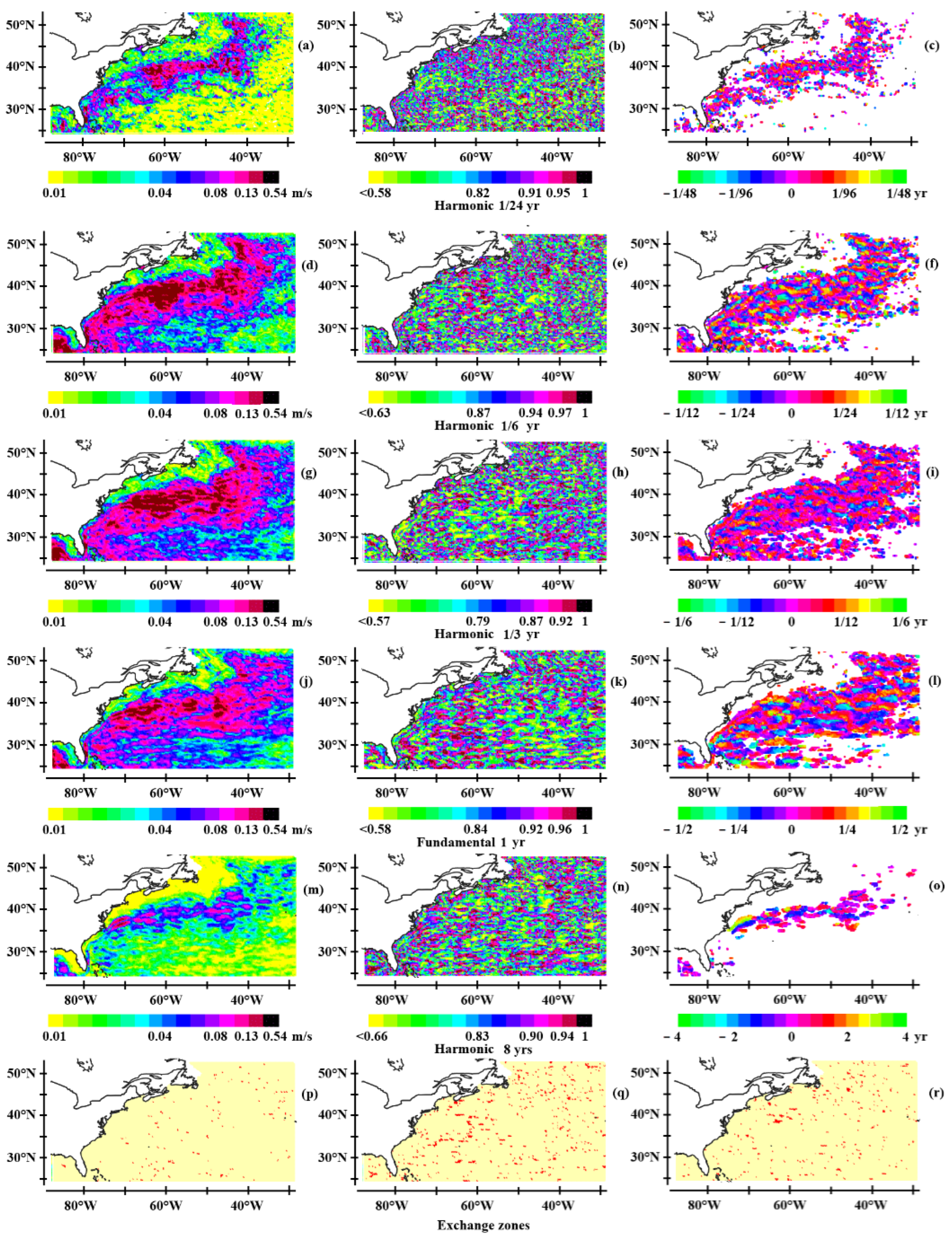
Figure 2.
Maximum velocity of the geostrophic current, averaged in the upper quantile (1/500th of the population) vs the period in – (a) the North Atlantic – (b) the South Atlantic – (c) the South Indian Ocean – (d) the North Pacific – (e) the South Pacific.
Figure 2.
Maximum velocity of the geostrophic current, averaged in the upper quantile (1/500th of the population) vs the period in – (a) the North Atlantic – (b) the South Atlantic – (c) the South Indian Ocean – (d) the North Pacific – (e) the South Pacific.
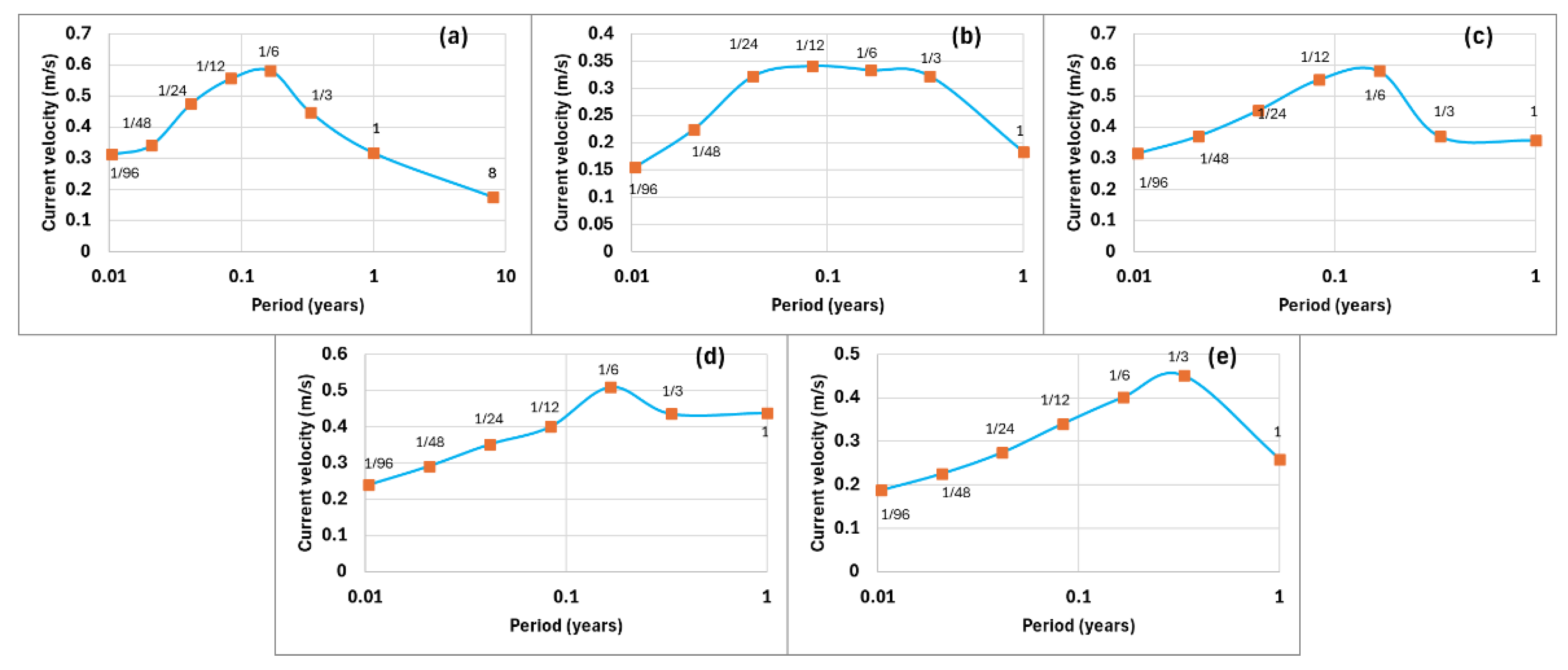
Figure 3.
North Atlantic: Anomalies of the 1/6 year period harmonics of 1) the geostrophic current velocity on 01/07/2004 (a, b, c) and 01/01/2005 (d, e, f) - 2) the sea surface temperature on 01/01/2006 (g, h, i) - 3) the geopotential height at 500 hPa time-averaged over a 2-month segment centered on 01/01/2006 (j, k, l): amplitude (a, d, g, j), coherence (b, e, h, k), and phase (c, f, i, l). The phases are represented where the amplitudes are the most significant in (c, f, i), and where the coherence is highest in (l). The references are at 38.5°N; 62.5°W for the geostrophic current velocity (a, b, c, d, e, f), at 37.5°N; 60.5°W for the sea surface temperature and the geopotential height (g, h, i, j, k, l).
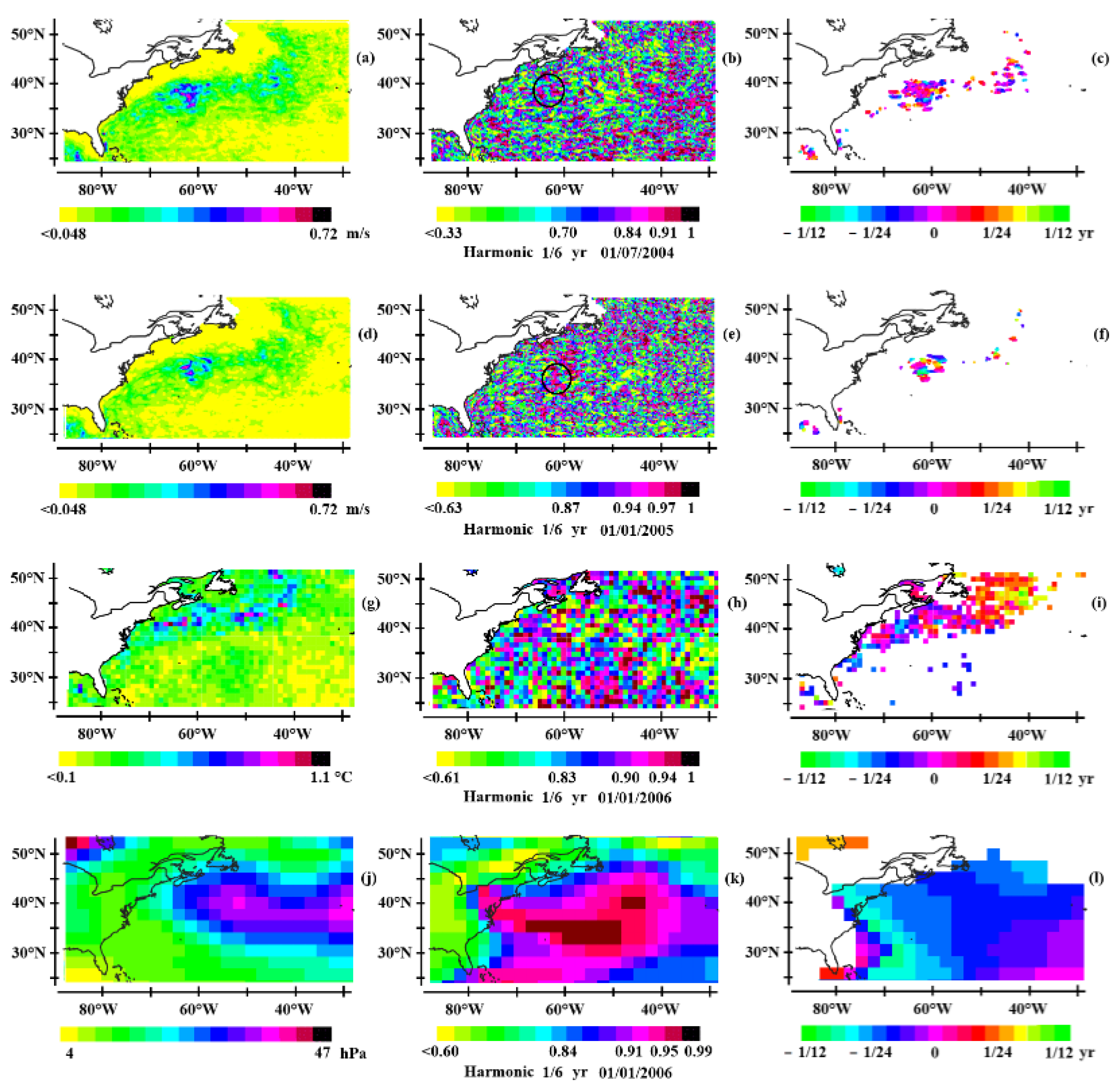
Figure 4.
South Atlantic: Anomalies of the 1/12 year period harmonics of 1) the geostrophic current velocity on 01/07/2004 (a, b, c) and 01/01/2005 (d, e, f) - 2) the sea surface temperature on 01/07/2005 (g, h, i) - 3) the geopotential height at 500 hPa time-averaged over a 2-month segment centered on 01/07/2005 (k, l, m): amplitude (a, d, g, j), coherence (b, e, h, k), and phase (c, f, i, l). Same convention for the representation of the phase as in Figure 3. The references are at 40°S; 50°W for the geostrophic current velocity (a, b, c, d, e, f), at 42.5°S; 52.5°W for the sea surface temperature and the geopotential height (g, h, i, j, k, l).
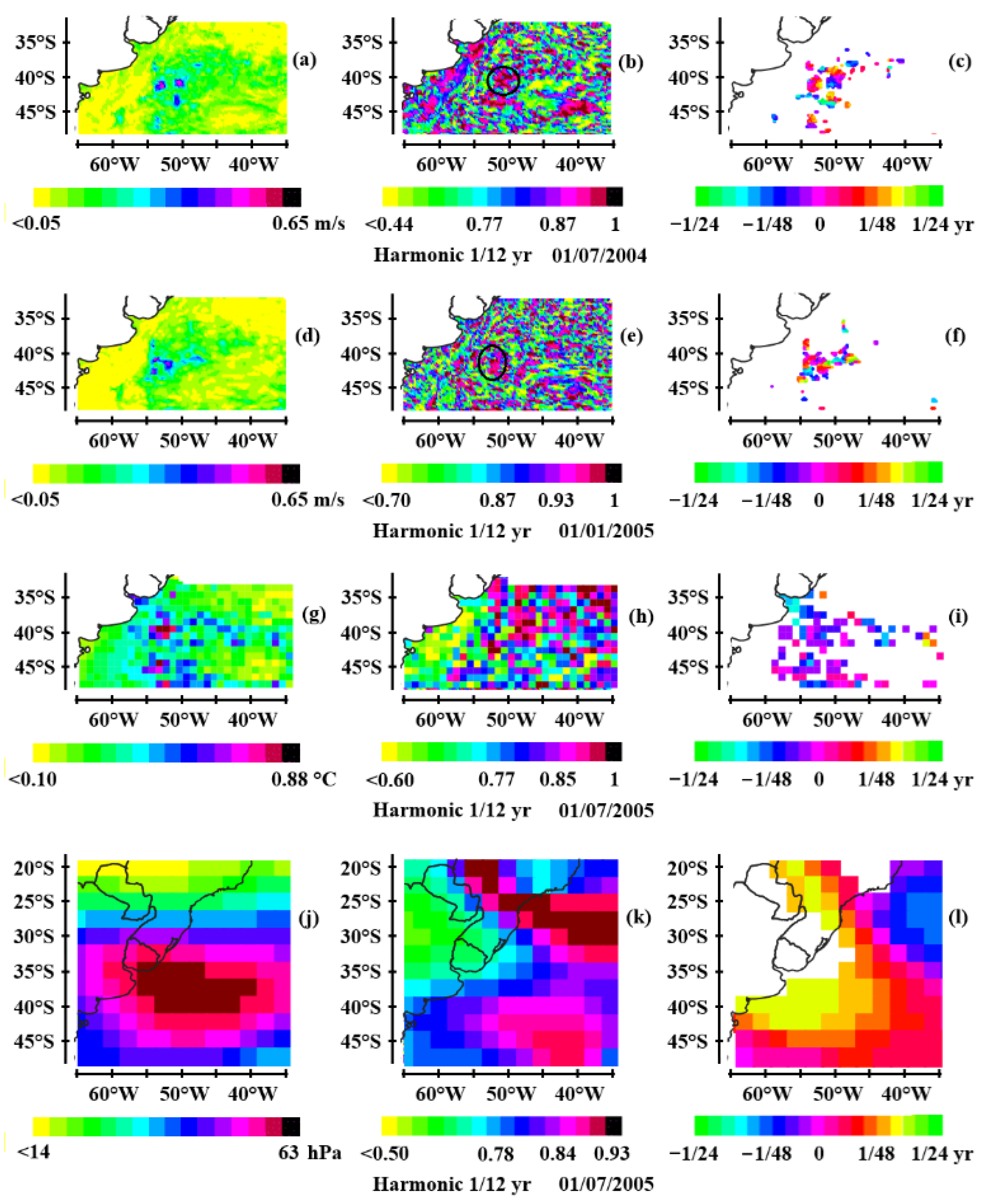
Figure 5.
Indian Ocean: Anomalies of the 1/12 year period harmonics of 1) the geostrophic current velocity on 01/01/2005 (a, b, c) - 2) the sea surface temperature on 01/07/2005 (d, e, f) - 3) the geopotential height at 500 hPa time-averaged over a 2-month segment centered on 01/07/2005 (k, l, m): amplitude (a, d, g), coherence (b, e, h), and phase (c, f, i). Same convention for the representation of the phase as in Figure 3. The references are at 38°S; 35°E for the geostrophic current velocity (a, b, c), at 39.5°S; 34.5°E for the sea surface temperature and the geopotential height (d, e, f, g, h, i).
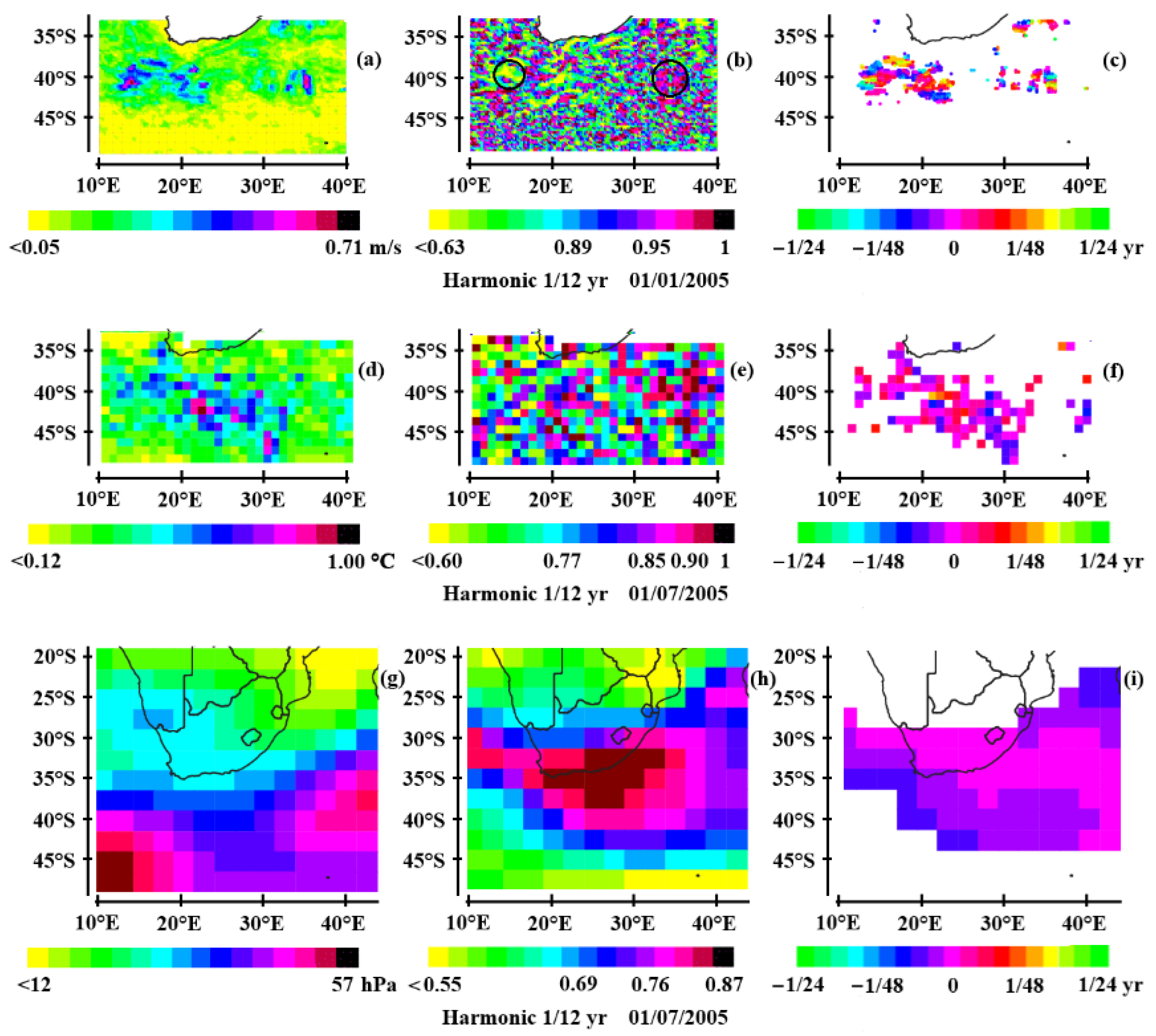
Figure 6.
South Pacific: Anomalies of the 1/3 year period harmonics of 1) the geostrophic current velocity anomalies on 01/07/2004 (a, b, c) and 01/01/2006 (d, e, f) - 2) the sea surface temperature on 01/07/2004 (g, h, i) - 3) the geopotential height at 500 hPa time-averaged over a 2-month segment centered on 01/07/2004 (j, k, l): amplitude (a, d, g, j), coherence (b, e, h, k), and phase (c, f, i, l). Same convention for the representation of the phase as in Figure 3. The references are at 30°S; 162°E for the geostrophic current velocity (a, b, c, d, e, f), at 30.5°S; 155.5°E for the sea surface temperature and the geopotential height (g, h, i, j, k, l).
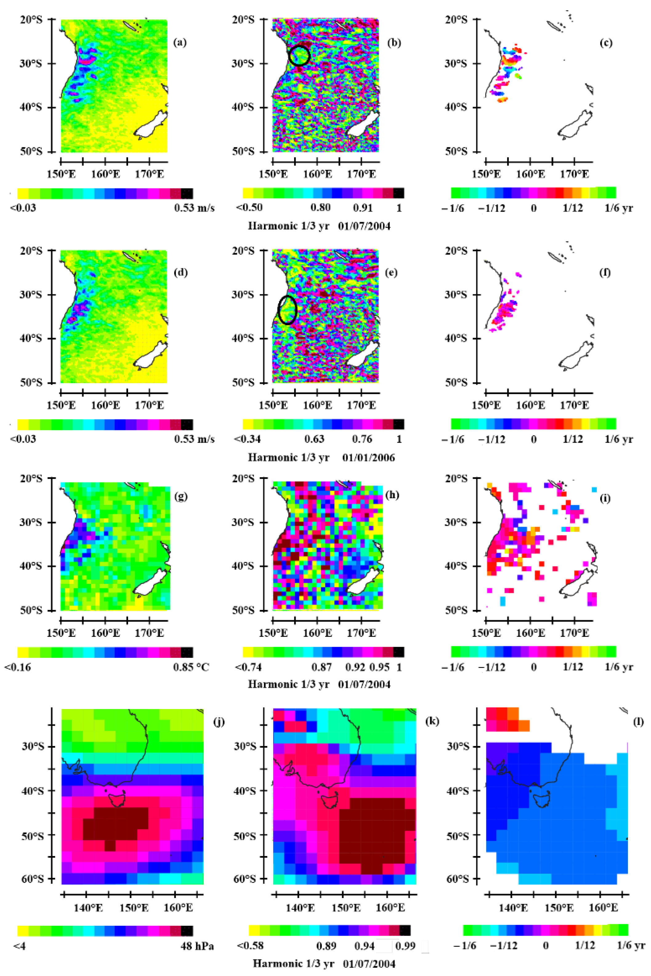
Figure 7.
North Pacific: Anomalies of the 1/6 year period harmonics of 1) the geostrophic current velocity on 01/07/2005 (a, b, c) - 2) the sea surface temperature on 01/01/2005 (d, e, f) - 3) the geopotential height at 500 hPa time-averaged over a 2-month segment centered on 01/01/2005 (k, l, m): amplitude (a, d, g), coherence (b, e, h), and phase (c, f, i). Same convention for the representation of the phase as in Figure 3. The references are at 35°N; 155°E for the geostrophic current velocity (a, b, c), at 34.5°N; 148.5°E for the sea surface temperature and the geopotential height (d, e, f, g, h, i).
Disclaimer/Publisher’s Note: The statements, opinions and data contained in all publications are solely those of the individual author(s) and contributor(s) and not of MDPI and/or the editor(s). MDPI and/or the editor(s) disclaim responsibility for any injury to people or property resulting from any ideas, methods, instructions or products referred to in the content. |
© 2025 by the authors. Licensee MDPI, Basel, Switzerland. This article is an open access article distributed under the terms and conditions of the Creative Commons Attribution (CC BY) license (http://creativecommons.org/licenses/by/4.0/).
Copyright: This open access article is published under a Creative Commons CC BY 4.0 license, which permit the free download, distribution, and reuse, provided that the author and preprint are cited in any reuse.


