
Submitted:
17 November 2025
Posted:
17 November 2025
You are already at the latest version
Abstract
Neuroscience adopts a multidimensional approach to decode thoughts and actions originating inside the brain, aka the Brain Computer Interface (BCI). However, achieving high accuracy in these decodings remains a challenge and an open research topic in BCI research. This study aims to enhance the accuracy of signal classification for identifying human emotional states. We utilized the publicly available EEG-Audio-Video (EAV) dataset that comprises EEG recordings from 42 subjects across five emotional categories. Our key contribution is to exploit the 2-dimensional contrast enhancement applied to the spectrogram for feature extraction, followed by classification using the EEGNet model. As a result, 12.5% improvement in classification accuracy over the baseline was achieved. This contribution demonstrates a potential advancement in BCI-based EEG signal processing in neuroscientific research.
Keywords:
adaptive contrast enhancement
; brain computer interface
; deep-learning
; emotional classification
; electroencephalography (EEG)
; short-time Fourier transform
1. Introduction
An electroencephalogram (EEG) records the electrical activity of the brain using surface electrodes attached to the scalp. The EEG has been employed for researching the Brain Computer Interfaces (BCIs) [1]. Neuroscience integrates several subfields, such as psychology & cognitive science, neuroimaging, and artificial intelligence (AI), to explore the functioning of the entire nervous system. Within neuroscience, BCI deals with communication between an individual’s brain signals and an external device not involving oral communication or motor functions [2]. BCI-EEG signals are characterized by their frequency, amplitude, waveform morphology, and spatial placement across scalp electrodes [3]. Typically, EEG signals span a frequency range of 0.1 Hz to 100 Hz and are categorized into five primary bandwidths (Figure 1): Delta (δ) with the range of 0.5–3.5 Hz, associated with deep sleep and comatose states; Theta (θ) with the range of 3.5–7.5 Hz, linked to creativity, stress, and deep meditation; Alpha (α) with the range of 7.5–12 Hz, predominant during relaxed and calm mental states; Beta (β) with the range of 13–30 Hz, observed during focused attention, visual processing, and motor coordination; and Gamma (γ) that has frequencies >30 Hz, which emerges during complex cognitive functions, motor execution, and multitasking [4].
The human brain is functionally divided into four major lobes: the frontal, temporal, parietal, and occipital lobes [6]. Each lobe is associated with a distinct set of structures, which correspond to specific neural functions. Figure 2 shows that the frontal lobe (Fp1, Fp2, AFz, F7, F3, Fz, F4, F8, FC5, FC1, FCz, FC2, and FC6) is primarily responsible for executive functions, including cognitive control, decision-making, and the regulation of emotional responses during task execution. The temporal lobe (T7, TP9, T8, and T10) plays a critical role in auditory processing and the perception of biological motion. The parietal lobe (P7, P3, Pz, P4, P8, PO9, PO10, CP1, CP2, CP5, and CP6) is largely involved in somatosensory processing, spatial representation, and tactile perception. Finally, the occipital lobe (O1, Oz, and O2) is primarily responsible for visual processing, particularly the perception and interpretation of visual stimuli.
Despite recent advancements, EEG-based BCI systems continue to face significant challenges, particularly with respect to low classification accuracy [7] and inter-subject variability [8]. The intra-user variability limitation refers to the phenomenon where EEG signals corresponding to the same cognitive task or thought can vary across different recording sessions for the same individual. In other words, the EEG pattern generated by a specific mental activity may not be identical when that activity is repeated at a later date or time [9].
This study aims to enhance the recognition accuracy of the emotional state of a person for BCI applications. It uses a publicly available EAV (EEG, Audio, Video) dataset [10] as a benchmark. The EAV dataset contains recordings from 42 subjects across five emotional classes: neutral, anger, happiness, sadness, and calmness [10]. Two EEG recordings from channel 0 and channel 5 for subject_1 are randomly depicted in Figure 3. The classification accuracy enhancement is achieved by refining the spectrogram feature extraction methods previously employed with the EEGNet architecture. The proposed methodology leverages the Short-Time Fourier Transform (STFT) that transforms EEG signals into a time-frequency representation. Later, adaptive contrast enhancement is introduced to achieve a better representation, enabling the EEGNet model to more accurately capture both temporal and spectral features.
This research paper is organized into five sections: Section II presents the literature review. Section III explains the research methodology design. Section IV describes the experiments. Section V explains the results and discussion. Finally, Section VI presents the conclusion, followed by the list of references.
2. Literature Review
One of the fundamental components of BCI technology is the ability to recognize emotional states within the brain. This process, often referred to as brain decoding, can be achieved through both invasive [11] and non-invasive [12] methods. Invasive BCIs involve the implantation of microelectronic devices beneath the scalp or directly into neural tissue such as the Electrocorticograph (ECOC) [13], offering high signal fidelity and accuracy. However, these methods present significant challenges, including the risk of infection, high cost, and surgical complexity [14]. In contrast, non-invasive techniques such as those based on EEG or functional near-infrared spectroscopy (fNIRS) [15] are widely adopted due to their safety, portability, and ease of use. While non-invasive approaches offer a more practical solution for everyday applications, they typically yield lower accuracy compared to invasive methods due to signal attenuation and noise. Nevertheless, EEG-based systems, in particular, have become central to the development of second-generation BCI technologies, offering a promising balance between usability and performance [16,17]. The task of decoding emotions from brain activity has attracted considerable attention from researchers. However, achieving high recognition accuracy remains a significant challenge, requiring substantial improvement. Nevertheless, recognizing and classifying EEG bio-signals is a complex task due to several inherent characteristics: high intra-subject variability, high dimensionality, non-stationarity, and a strong susceptibility to noise [18]. These challenges are further compounded when applying deep learning techniques to EEG-based emotion recognition. In particular, two major obstacles persist: the variability of emotional patterns across individuals (intra-subject variability) and the limited availability of labeled EEG datasets. Several studies on emotion recognition using EEG signals have been made publicly available. Notably, Feng et al. [18], proposed a method based on a pre-trained Vision Transformer for emotion recognition, evaluating its performance across four widely-used public datasets: SEED, SEED-IV, DEAP, and FACED. The cross-dataset emotion recognition accuracy achieved 93.14% on SEED, 83.18% on SEED-IV, 93.53% on DEAP, and 92.55% on FACED. The approach utilizes a transfer learning framework known as Pre-trained Encoder from Sensitive Data (PESD).
Another notable study, published in Nature [10], introduced the EAV (EEG-Audio-Video) dataset for emotion recognition in conversational contexts. This multimodal dataset incorporates three modalities—EEG, audio, and video—to model human emotions more comprehensively. Among these, EEG plays a central role. For the EEG component, the authors employed the SEED-IV dataset, which consists of 30-channel EEG recordings. A total of 42 participants took part in the study, each engaging in cue-based conversational scenarios designed to elicit five distinct emotional states: neutrality, anger, happiness, sadness, and calmness. Each participant contributed approximately 200 interactions, encompassing both listening and speaking tasks, resulting in a total of 8,400 interactions across all participants. For EEG data acquisition, the BrainAmp system (Brain Products, Munich, Germany) was used. EEG signals were collected via Ag/AgCl electrodes placed at standardized scalp locations: Fp1, Fp2, F7, F3, Fz, F4, F8, FC5, FC1, FC2, FC6, T7, C3, Cz, C4, T8, CP5, CP1, CP2, CP6, P7, P3, Pz, P4, P8, PO9, O1, Oz, O2, and PO10. Data were sampled at 500 Hz, with reference electrodes placed at the mastoids and grounding via the Afz electrode. The electrode impedance was maintained below 10 kΩ to ensure data quality. The EEG recordings were initially stored in BrainVision Core Data Format and later converted to MATLAB (.mat) format for preprocessing and analysis. Emotion recognition performance for each modality was evaluated using deep neural network (DNN) models. The best classification accuracy achieved for EEG-based emotion recognition using this dataset was approximately 60%. We will use these results as a benchmark as we aim to enhance the classification accuracy of the EAV dataset.
Other researchers have classified EEG into three classes: happy, neutral, and sad, as reported in [19]. Using an SVM classifier with time-frequency features, an accuracy of 88.93% was achieved. Various EEG datasets are designed to study emotional responses under varying experimental conditions. The DEAP dataset [20] records 32-channel EEG from 32 participants during music video stimulation, annotated with continuous dimensions (valence, arousal, dominance, and liking), making it suitable for dimensional emotion modeling. The SEED series [21] employs 64-channel EEG and movie clips to induce discrete emotions such as positive, negative, and neutral; after that, happy, sad, and fear in SEED-IV/V across 15 subjects, facilitating categorical emotion classification studies. In contrast, the DREAMER dataset [22] uses 14-channel EEG from 23 subjects watching film clips, providing self-reported valence, arousal, and dominance ratings, balancing practicality with robust affective annotations. Another MPED dataset (Song et al., 2019) [23] extends emotional descriptors to include arousal, valence, and discrete emotional states (DES) via 62-channel EEG.
3. Materials and Methods
The signal processing and classification of emotional EEG waves involve several processing steps, including band-pass filtering, downsampling, and a reshaping process. Following preprocessing, STFT [24,25] is applied as a feature extraction technique to enhance the signal’s representational characteristics. Unlike a standard Fourier Transform, which assumes signal stationarity, the STFT operates by dividing the continuous EEG signal into brief, sequential time segments using a sliding window function. This allows for the computation of a local Fourier spectrum for each segment, effectively capturing the temporal evolution of spectral power across key frequency bands (delta, theta, alpha, beta, gamma). The resultant time-frequency representation (TFR) provides a highly informative feature set that preserves crucial information about both the timing and the frequency content of neural oscillations and transient events. Then, the adaptive contrast enhancement (ACE) process is applied. Later, a two-dimensional feature matrix is prepared for subsequent advanced analysis within the EEGLab environment, which employs a deep learning training model to classify specific cognitive states. The preprocessing pipeline and the overall model architecture are depicted in the general block diagram as shown in Figure 4.
In this study, EEG data consisting of 42 subjects was retrieved from the public EAV Dataset [10]. Each record has two files: an EEG data file that contains raw EEG signals and a corresponding label file containing class annotations. The EEG signals are represented as , where the number of time samples over of recording at 500Hz, is the number of channels, and is the number of trials. Labels are stored as a one-hot encoded matrix: , where is the number of classes. The input dataset for each subject has dimensions. The data were organized into segments, with each segment representing a trial of EEG recordings across multiple channels. The preprocessing pipeline consisted of several steps to prepare the EEG data for classification. The first step applied bandpass filtering (BPF) to retain frequencies between 3 Hz and 50 Hz, resulting in the filtered signal , given by equation:
Next, the filtered EEG signal were down-sampled from to using polyphase resampling [26] to reduce computational complexity, as given by equation:
Where represents the downsampled signal. Then, the reshaped data is segmented and transposed into a format suitable for analysis, resulting in a shape . Then, segmentation and reshaping processes are applied, in which the down-sampled signals were segmented into trials and then reshaped into a tensor , where is the number of trials, is the number of downsampled time points per trial, and . Where .
The down-sampled signals are reshaped and transposed to align with the segmentation requirements of the classification model. Five specific class labels: were randomly selected for classification. One-hot encoding was applied to represent the class labels as in equation:
In the above, , where is the number of selected trails. Accordingly, the input dataset has the dimensions, , 400 for trials, for channels, and for time points for the EEG signal with the corresponding Labels, . Next, the STFT was applied to the EEG dataset, as a key methodological improvement that could enhance the EEG signal recognition accuracy by providing time-frequency localization
3.1. Short-Time Fourier Transform (STFT) Feature Extraction
Given an input EEG dataset , where is the number of trials is the number of channels, is the number of time samples, the STFT was applied to each trial. The STFT parameters are: (the sampling frequency in Hz), (the segment length), and (the number of overlapping samples between consecutive segments). The STFT is applied to each one-dimensional EEG signal , where represents the time-domain signal for trial , channel and the sam
ple index . The STFT is defined as equation:
where:
is the complex-valued STFT coefficient for frequency_bin ( and time_bin (;
is a window function of length ;
indexes the frequency_bins assuming positive frequencies for real-valued signals; and,
indexes the time bins, where is the number of time_bins.
To boost the output, the absolute value is obtained from the complex-valued STFT coefficients: . The resulting STFT magnitude is organized into a four-dimensional array , where: is the number of frequency_bins including zero frequency and Nyquist frequency for even , and is the number of time_bins. For each trial and chancel ,the STFT magnitude is computed, and the result are stacked as:.
It may be noted that the choice of the window function and parameters and affects the time-frequency resolution trade-off. A larger provides better frequency resolution but poorer time resolution, while a larger increases the number of time_bins, improving temporal smoothness. The sampling frequency determines the frequency resolution with frequency_bins corresponding tofor .
To facilitate compatibility with the convolutional neural networks (CNNs) within the EEGLAB environment, the 2D time-frequency representation is transformed into a 1D feature vector. This is achieved through a flattening operation, which reshapes the spectrogram matrix, comprising frequency_bins and time_bins into a contiguous vector of length . Consequently, the final feature set, denoted as STFT_Cof, encapsulates the entire constellation of magnitude values from the STFT for each single channel in each subject, thereby rendering the rich time-frequency structure into a format suitable for the EEGLAB. Now, the dataset is ready to be fed into the EEGnet for training and building the future reference model. Thus the final tensor .
3.2. Adaptive Contrast Enhancement (ACE)
The adaptive local spectral contrast enhancement (ACE) is used to improve the interpretability and feature salience of time-frequency representations [27,28]. In this study, ACE is used to mitigate the low contrast of the STFT spectrogram features. This is accomplished by normalizing the spectrogram based on local statistics within a defined neighborhood .
Let denote an input spectrogram and denote the enhanced spectrogram. Let neighborhood and around each point be defined, where the kernel is specified by the neighborhood_size as a hyperparameter. The local statistical estimation includes the local mean and local standard eviation, which are estimated within this neighborhood using uniform filters. The local mean is computed as equation:
where is the number of points in the neighborhood. The local standard which measures local spectral contrast (texture) is derived from the local mean of squares as equation:
Each point in the spectrogram is then normalized (Z-score) by subtracting the local mean and dividing by the local standard deviation as equation:
A small constant is added for numerical stability and in some cases to prevent division by zero. This operation effectively stretches the local dynamic range, boosting components that stand out from their local background. To map the enhanced data back to a physically meaningful range, a min-max rescaling is applied to normalize within the range [0, 1] as equation:
It is then rescaled to the original amplitude range of the input spectrogram , to preserve the global amplitude relationships while maintaining the enhanced local contrast as equation:
3.3. Deep Learning EEGNet Classifier
After extracting the features for all subjects and channels, the enhanced data is fed into the CNN, which consists of 14 layers arranged in two blocks. Table 1 details the sequential layer architecture of EEGNet [29], a convolutional neural network (CNN). Each block consists of a sequence of layers including convolution, normalization, ReLU activation, and average pooling, with their corresponding hyperparameter configurations specified in the table.
The model is trained with the Adam optimizer and categorical cross-entropy loss function. To maintain the cross-validation, the STFT dataset is split into two sets: 50% for training and the other 50% for testing. The 50% training dataset is further subdivided into training (70%) and validation (30%) sets. The model was trained for 100 epochs with a batch size of 32, and performance was monitored on the validation set. The choice of window function and parameters and affects the time-frequency resolution trade-off. These parameters were selected following experimentation for achieving better accuracy. The Model’s performance was evaluated on the blind test set using accuracy and the weighted F1-score. A confusion matrix was computed for each subject to assess classification performance across the five classes. The confusion matrices were summed across all subjects to obtain an aggregate performance metric. Average accuracy and F1-scores were calculated to summarize the model’s effectiveness. The results were averaged across all 42 subjects. The summed confusion matrix provided insights into the model’s classification performance across the selected classes. In the experiments, the adjustable parameters include the number of classes Nclasses = 5, dropout rate δ = 0.5, filters F1 = 8, depth multiplier D = 2, filters F2 = 16, and normalization rate η = 0.25. Dropout type is either SpatialDropout2D or Dropout.
4. Results and Discussion
Spectrograms based on the STFT for selected EEG signals, such as those from subjects 2 and 3, are shown in Figure 5. In which Figure 5 (a) depicts EEG signals related to subject 2 across three channels: 0, 5, and 10. Their spectrogram for each channel is represented as a time bin on the x-axis and a frequency bin on the y-axis, with spectral power indicated by color intensity. From the image, it is obvious that the higher amplitude signals have higher power spectrum signals in their frequency domain. This process can represent the signals more effectively and provide an abstract representation of the signals’ temporal changes over time, leading to a better understanding by the classifier. Similarly, Figure 5 (b) shows the EEG signals for subject 3, using the three channels 0, 5, and 10, in both the time and frequency domains. Remarkably, this method’s capacity underscores revealing energy distribution across frequency bands over time that offers an informative abstraction of temporal dynamics, enhancing feature discriminability for subsequent classification.
A limitation of the STFT technique is its Fixed Time-Frequency Resolution since the STFT uses a fixed window size . The choice of window function mitigates but does not eliminate this issue. Also, it could have sensitivity to parameter selection because the performance of the STFT depends heavily on the choice of and, for the window function. Suboptimal parameters can lead to poor resolution or artifacts, requiring domain expertise or empirical tuning. Eventually, tensor can be high-dimensional, especially for large , or , that is increasing memory and computational requirements for downstream processing
4.1. Signal Enhancement Using STFT with ACE
Figure 6 visualizes the effect of the adaptive spectral contrast enhancement on the STFT original and enhanced STFT of subject 2 and subject 3 using randomly selected channels 5 and 10 from each subject. The ACE has three main effects as follows:
- First, the increased contrast, which means that the high and low frequency bin regions in the spectrogram are clearer in the enhanced versions. This makes it easier for the machine learning to distinguish between different frequency components and their changes over time.
- Secondly, spectral features are sharper or more defined in the enhanced plots. And The third effect is background noise elimination by amplifying the relevant signal components while relatively suppressing the less important background noise.
Furthermore, it is easily assessed that the difference between Figure 6 (a), the original STFT, and Figure 6 (b), the enhanced STFT, is subjective. Indeed, ACE has limitations that need to be considered. For example, the normalization process can create artifacts around strong, isolated features, where the local standard deviation is very low just outside the feature's boundary. Besides, the ACE method assumes local stationarity within the window. It may perform poorly with highly non-stationary EEG interfering signals.
The choice of the hyperparameter named neighborhood_size is essential for improving the EEG signal representations. It is a trade-off, because if a small window, for instance, , the process captures very fine-grained, high-frequency texture. Therefore, this is useful for enhancing narrow spectral lines but may also extract high-frequency noise. Conversely, if large windows are configured, for instance, , the process captures broader spectral trends. This is effective for enhancing larger structures, such as a formant's spectral envelope, but may overlook finer details. Overall, the enhancement aims to make the important spectral characteristics of the EEG data more visually prominent, which can be beneficial for subsequent analysis or input into a machine learning model like EEGNet.
4.2. Recognition Accuracy
The classification accuracy is assessed by exploiting the confusion matrix (CM) [30].In the case of two classes, CM has four parameters: True Positive (TP), True Negative (TN), False Positive (FP), and False Negative (FN), as illustrated in Table 2.
In this paper, the proposed classifier is evaluated by its accuracy and F1 score, in which their formulas are listed below equations:
As this research involves five emotional categories, the standard confusion matrix is extended from two to five classes. The idea is to consider one class as true and the remaining four as false. For example, if the second class is considered true, the first, third, fourth, and fifth are deemed false. Figure 7. presents a comparative analysis of classification accuracy for 42 subjects, contrasting the performance of original EEG data (black), pre-processed EEG dataset using Short-Time Fourier Transform (STFT) feature extraction (orange), and the STFT with the ACE processing (green). The x-axis represents the subject index (1–42), while the y-axis denotes accuracy values ranging from 0 to 1.
The plot reveals variability in the accuracy across subjects, with some showing significant improvement after STFT with the ACE dataset processing, while others exhibit minimal change or slight degradation. Figure 8 presents a comparative analysis of classification accuracy based on F1-score for 42 subjects, contrasting the performance of original EEG data (black), pre-processed EEG dataset using STFT feature extraction (orange), and the STFT with the ACE processing (green). The x-axis represents the subject index (1–42), while the y-axis denotes accuracy values ranging from 0 to 1. There is an improvement after STFT with the ACE dataset processing compared with the original EEG dataset, while others exhibit minimal change or slight degradation.
4.3 Comparison of Classification Accuracies
Table 3 contains the recognition accuracy results of an EEG for five emotional classes: neutrality, anger, happiness, sadness, and calmness. Eight experiments were run for training and testing, and their averages have been calculated. Table III demonstrates a clear performance where the proposed method (STFT+ Adaptive Contrast Enhancement + EEGNet) consistently achieves the highest accuracy with an average of up to 72.5%, outperforming both the approach consisting of STFT + EEGNet at an average of up to 70.84%, and the baseline EEGNet alone has the classification accuracy as an average of up to 59.94% (which is similar to the accuracy published in original dataset [10]).
The substantial increase from the baseline to STFT-enhanced models confirms the critical importance of time-frequency features for EEG analysis, while integrating a small improvement from adding ACE signal preprocessing as an effective refinement technique that enhances feature discriminability in spectrograms. The resulting low variance across all eight experimental runs confirms the statistical robustness of these improvements, solidifying the conclusion that each processing stage (particularly the ACE approach) meaningfully contributes to more accurate and reliable EEG classification.
Table 4 illustrates the confusion matrix related to the STFT with the ACE preprocessing. For the 42 subjects, each of which has 1680 samples per class, and 1 subject has 40 samples per class, as listed in the table. Because each subject has 200 instances entered in the testing (40 instances/class). The model demonstrates strong overall performance for a complex 5-class problem. The high values along the main diagonal (1195, 1195, 1287, 1294, 1130) summed to 6,101 correct predictions, while off-diagonal elements represent misclassifications. The overall accuracy is given as 6,101/8,400 = 72.6%, which reflects the correct predictions divided by the number of samples (5 classes × 1680 instances).
Figure 9 depicts the evaluation across all 42 subjects, featuring three distinct confusion matrices. The first CM corresponds to the model testing on the 200 instances for each subject's original dataset, establishing a baseline performance. The second matrix presents the testing results utilizing STFT pre-processing on a held-out set of 200 instances, representing a blind testing scenario. The third matrix illustrates the accuracy achieved by integrating STFT with ACE pre-processing. A comparative analysis reveals that the principal diagonal of the third confusion matrix (proposed method) contains the highest instances of correct predictions, demonstrating a superior classification accuracy and an enhanced emotional recognition rate attributable to the combined STFT-ACE preprocessing pipeline.
The graph in Figure 10, illustrates the relationship between classification accuracy and neighborhood size as a hyperparameter associated with ACE preprocessing. As it is shown that the accuracy demonstrates notable sensitivity to this parameter, initially increasing to an apparent optimum between neighborhood sizes of 10 and 11, where peak performance of approximately 73% is attained. Beyond this peak, a consistent decrease in accuracy is observed when the neighborhood size increases to 14, suggesting that larger neighborhoods introduce non-discriminative information that degrades the model's performance.
4.4. SHAP Channel Importance Analysis
To highlight which active EEG channels contribute more to building the model than others, SHAP (Shapley Additive exPlanations) analysis is applied. SHAP is based on mean absolute SHAP values to provide a quantitative assessment of the contribution of EEG channel to the predictive output of the trained model [31]. According to Figure 11, channels with taller bars are more influential in determining the model's predictions compared to channels with shorter bars. A high mean absolute SHAP value for a channel suggests that the information contained within the signal from that channel significantly contributes to the model's ability to discriminate between the different classes. Conversely, channels with low mean absolute SHAP values are less effective for the model's performance.
Based on the mean absolute SHAP values presented in Figure 10, and the sorted list of channels by importance, it is clear that channels: channel 15, channel 29, channel 10, channel 1, and channel 2 exhibit higher mean absolute SHAP values compared to other channels. This means that the information acquired by these specific channels is more critical for the model to classify the emotional EEG data. On the contrary, channels with shorter bars, such as channel 9, channel 21, and channel 26, have lower mean absolute SHAP values, indicating they are less influential in the model's decision-making process for this task and dataset. Therefore, the dataset could be reduced without a big impact on the model accuracy. Analyzing the spatial distribution of these important channels on an EEG cap could help neuroscientists to locate which brain regions (channels) are expected to be relevant for emotion processing. In addition, SHAP can be used in the future to adjust the accuracy by applying channel reduction based on SHAP mean absolute values, and then to pipeline it with the STFT along with the ACE for better accuracy and efficient computation.
5. Conclusions
Despite recent improvements in BCI, the biggest potential challenge in EEG-based BCI systems remains the limited recognition rate and the ability to represent an individual's neural patterns for accurate and reliable classification. This paper proposed an efficient methodology aimed at enhancing classification accuracy through a robust pipeline for EEG signal processing and classification. The proposed approach leverages the STFT of non-stationary EEG signals with ACE to amplify high-frequency details by attenuating low-frequency components. The proposed method achieved an average accuracy of 72.50%. This represents a 12.55% improvement over the baseline accuracy of 60% reported in the original EAV study. The proposed methodology has the potential to enhance EEG recognition across multiple fields. Future work will focus on optimizing key parameters, such as STFT windowing and ACE neighborhood size, and explore the use of SHAP-based channel interpretation for feature selection to facilitate the deployment of this methodology on lightweight embedded systems.
Informed Consent Statement
Not applicable.
Data Availability Statement
The data presented in this study are available upon. For more details: https://www.nature.com/articles/s41597-024-03838-4
Complete code for the proposed work can be accessed:https://drive.google.com/file/d/1NJm_jgrPXaWMm8aKHcDGH2PQbbVhP6Sc/view?usp=sharing
Conflicts of Interest
The authors declare no conflicts of interest.
References
- Bastos, N.S.; Marques, B.P.; Adamatti, D.F.; Billa, C.Z. Analyzing EEG signals using decision trees: A Study of modulation of amplitude. Comput. Intell. Neurosci. 2020, 2020, 1–11. [Google Scholar] [CrossRef] [PubMed]
- S. Machado et al., "Interface cérebro-computador: novas perspectivas para a reabilitação," vol. 17, no. 4, pp. 329-235, 2009.
- V. Jayaraman, S. V. Jayaraman, S. Sivalingam, and S. Munian, "Analysis of Real Time EEG Signals," ed, 2014.
- Ghosh, R.; Deb, N.; Sengupta, K.; Phukan, A.; Choudhury, N.; Kashyap, S.; Phadikar, S.; Saha, R.; Das, P.; Sinha, N.; et al. SAM 40: Dataset of 40 subject EEG recordings to monitor the induced-stress while performing Stroop color-word test, arithmetic task, and mirror image recognition task. Data Brief 2022, 40, 107772. [Google Scholar] [CrossRef] [PubMed]
- Pandey, P.; Tripathi, R.; Miyapuram, K.P. Classifying oscillatory brain activity associated with Indian Rasas using network metrics. Brain Informatics 2022, 9, 1–20. [Google Scholar] [CrossRef] [PubMed]
- <b>6. </b>S. Jacobson, S. S. Jacobson, S. Pugsley, and E. M. Marcus, "Cerebral cortex functional localization," in Neuroanatomy for the Neuroscientist: Springer, 2025, pp. 347-379.
- S. Kumar and A. J. S. P. S. Sharma, "Advances in non-invasive EEG-based brain-computer interfaces: Signal acquisition, processing, emerging approaches, and applications," pp. 281-310, 2025.
- S. Thakur et al., "Exploring the Evolution of Feature Extraction Methods in Brain–Computer Interfaces (BCIs): A Systematic Review of Research Progress and Future Trends," vol. 15, no. 3, p. e70040, 2025.
- Barrows, P.; Van Gordon, W.; Gilbert, P. Current trends and challenges in EEG research on meditation and mindfulness. Discov. Psychol. 2024, 4, 1–22. [Google Scholar] [CrossRef]
- Lee, M.-H.; Shomanov, A.; Begim, B.; Kabidenova, Z.; Nyssanbay, A.; Yazici, A.; Lee, S.-W. EAV: EEG-Audio-Video Dataset for Emotion Recognition in Conversational Contexts. Sci. Data 2024, 11, 1–15. [Google Scholar] [CrossRef] [PubMed]
- Merk, T.; Köhler, R.M.; Brotons, T.M.; Vossberg, S.R.; Peterson, V.; Lyra, L.F.; Vanhoecke, J.; Chikermane, M.; Binns, T.S.; Li, N.; et al. Invasive neurophysiology and whole brain connectomics for neural decoding in patients with brain implants. Nat. Biomed. Eng. 2025, 1–18. [Google Scholar] [CrossRef] [PubMed]
- S. d'Ascoli et al., "Decoding individual words from non-invasive brain recordings across 723 participants," 2024.
- Leuthardt, E.C.; Moran, D.W.; Mullen, T.R.J.F.I.N. "Defining surgical terminology and risk for brain computer interface technologies. Front. Neurosci. 2021 15, 599549. [CrossRef] [PubMed]
- Arico, P.; Borghini, G.; Di Flumeri, G.; Sciaraffa, N.; Colosimo, A.; Babiloni, F. Passive BCI in operational environments: insights, recent advances, and future trends. IEEE Trans. Biomed. Eng. 2017, 64, 1431–1436. [Google Scholar] [CrossRef] [PubMed]
- Nia, A.F.; Tang, V.; Talou, G.D.M.; Billinghurst, M. Decoding emotions through personalized multi-modal fNIRS-EEG Systems: Exploring deterministic fusion techniques. Biomed. Signal Process. Control. 2025, 105, 107632. [Google Scholar] [CrossRef]
- Zhang, M.; Qian, B.; Gao, J.; Zhao, S.; Cui, Y.; Luo, Z.; Shi, K.; Yin, E. Recent Advances in Portable Dry Electrode EEG: Architecture and Applications in Brain-Computer Interfaces. Sensors 2025, 25, 5215. [Google Scholar] [CrossRef] [PubMed]
- Tam, N.D. A second-generation non-invasive brain–computer interface (BCI) design for wheelchair control. Acad. Eng. 2025, 2. [Google Scholar] [CrossRef]
- Wang, F.; Tian, Y.-C.; Zhou, X. Cross-dataset EEG emotion recognition based on pre-trained Vision Transformer considering emotional sensitivity diversity. Expert Syst. Appl. 2025, 279. [Google Scholar] [CrossRef]
- Sun, H.; Wang, H.; Wang, R.; Gao, Y. Emotion recognition based on EEG source signals and dynamic brain function network. J. Neurosci. Methods 2024, 415. [Google Scholar] [CrossRef]
- Koelstra, S.; Muhl, C.; Soleymani, M.; Lee, J.-S.; Yazdani, A.; Ebrahimi, T.; Pun, T.; Nijholt, A.; Patras, I. DEAP: A database for emotion analysis ;using physiological signals. IEEE Trans. Affect. Comput. 2011, 3, 18–31. [Google Scholar] [CrossRef]
- Zheng, W.-L.; Zhu, J.-Y.; Lu, B.-L. Identifying stable patterns over time for emotion recognition from EEG. IEEE Trans. Affect. Comput. 2017, 10, 417–429. [Google Scholar] [CrossRef]
- Katsigiannis, S.; Ramzan, N. DREAMER: A database for emotion recognition through EEG and ECG signals from wireless low-cost off-the-shelf devices. IEEE J. Biomed. Heal. Informatics 2017, 22, 98–107. [Google Scholar] [CrossRef] [PubMed]
- Song, T.; Zheng, W.; Lu, C.; Zong, Y.; Zhang, X.; Cui, Z. MPED: A multi-modal physiological emotion database for discrete emotion recognition. IEEE Access 2019, 7, 12177–12191. [Google Scholar] [CrossRef]
- Mateo, C.; Talavera, J.A. Bridging the gap between the short-time Fourier transform (STFT), wavelets, the constant-Q transform and multi-resolution STFT. Signal, Image Video Process. 2020, 14, 1535–1543. [Google Scholar] [CrossRef]
- N. R. Babu and V. J. I. A. Viswanathan, "MFENet: A Multi-Feature Extraction Network for Enhanced Emotion Detection Using EEG and STFT," 2025.
- Harris, F. Polyphase Interpolators with Reversed Order of Up-Sampling and Down-Sampling. 2021 55th Asilomar Conference on Signals, Systems, and Computers. LOCATION OF CONFERENCE, United StatesDATE OF CONFERENCE; pp. 918–924.
- Zhang, W.; Zhuang, P.; Sun, H.-H.; Li, G.; Kwong, S.; Li, C. Underwater image enhancement via minimal color loss and locally adaptive contrast enhancement. IEEE Trans. Image Process. 2022, 31, 3997–4010. [Google Scholar] [CrossRef] [PubMed]
- I. V. Safonov, I. V. Kurilin, M. N. Rychagov, and E. V. Tolstaya, "Adaptive global and local contrast enhancement," in Adaptive Image Processing Algorithms for Printing: Springer, 2017, pp. 1-39.
- V. Pandey, N. Panwar, A. Kumbhar, P. P. Roy, and M. Iwamura, "Enhanced Cross-Task EEG Classification: Domain Adaptation with EEGNet," in International Conference on Pattern Recognition, 2025, pp. 354-369: Springer.
- F. Hu et al., "STRFLNet: Spatio-Temporal Representation Fusion Learning Network for EEG-Based Emotion Recognition," 2025.
- B. Mouazen et al., "Transparent EEG Analysis: Leveraging Autoencoders, Bi-LSTMs, and SHAP for Improved Neurodegenerative Diseases Detection," vol. 25, no. 18, p. 5690, 2025.
Figure 1.
EEG signals displaying brain rhythms characterized by distinct frequency bands: Delta, Theta, Alpha, Beta, and Gamma [5].
Figure 1.
EEG signals displaying brain rhythms characterized by distinct frequency bands: Delta, Theta, Alpha, Beta, and Gamma [5].
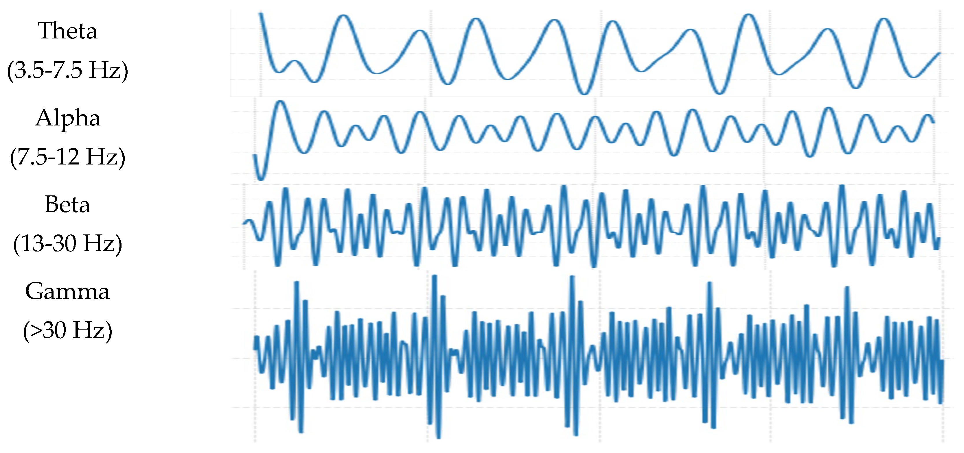
Figure 2.
Placement of the electrodes for a 32-channel EEG across all four cerebral lobes—frontal, temporal, parietal, and occipital [4].
Figure 2.
Placement of the electrodes for a 32-channel EEG across all four cerebral lobes—frontal, temporal, parietal, and occipital [4].
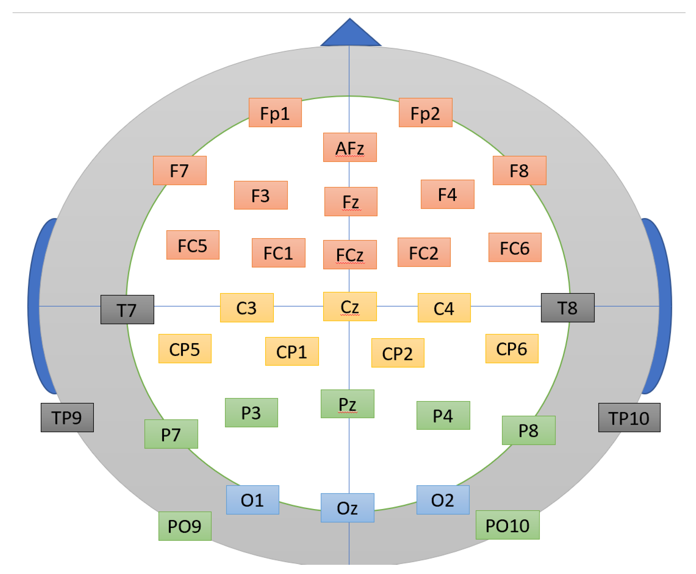
Figure 3.
Randomly picked EEG signal samples from the EAV dataset: (a) Subject_1: channel_0, (b) Subject_1: channel_5.
Figure 3.
Randomly picked EEG signal samples from the EAV dataset: (a) Subject_1: channel_0, (b) Subject_1: channel_5.

Figure 4.
General block diagram for the proposed methodology for emotional EEG signal classification.
Figure 4.
General block diagram for the proposed methodology for emotional EEG signal classification.
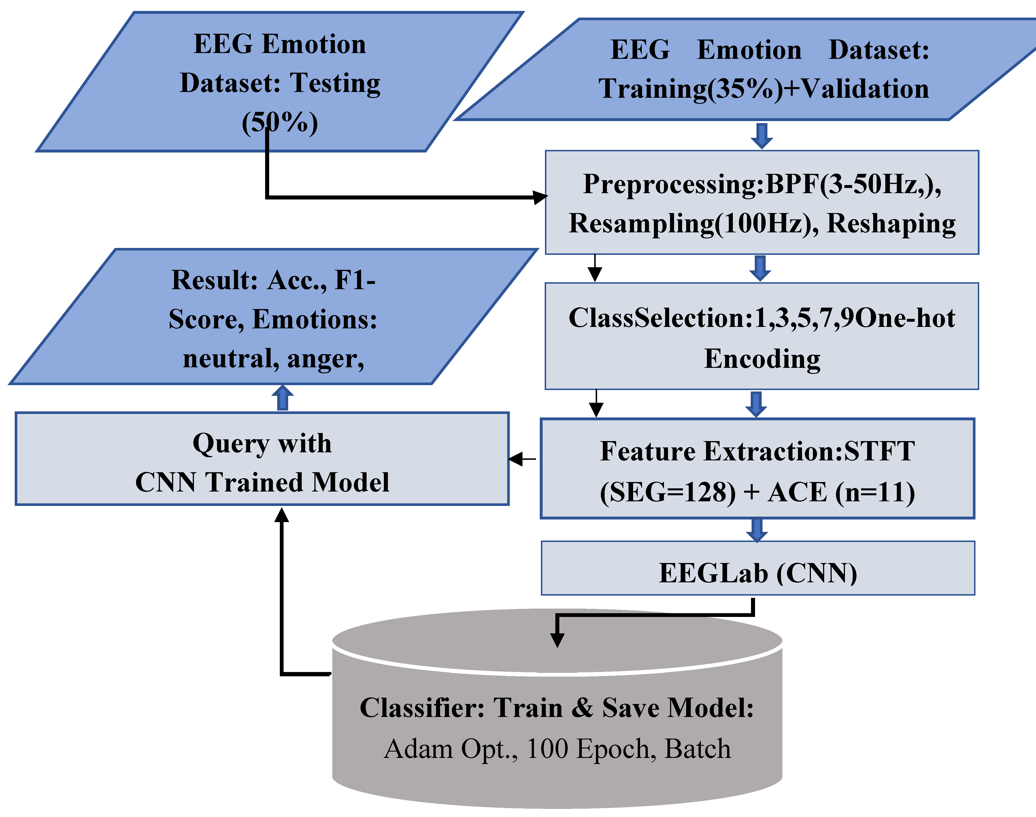
Figure 5.
EEG signal waveform in the time domain and following STFT: Channels 0, 5, and 10, (a) Subject 2, (b) Subject 3.
Figure 5.
EEG signal waveform in the time domain and following STFT: Channels 0, 5, and 10, (a) Subject 2, (b) Subject 3.
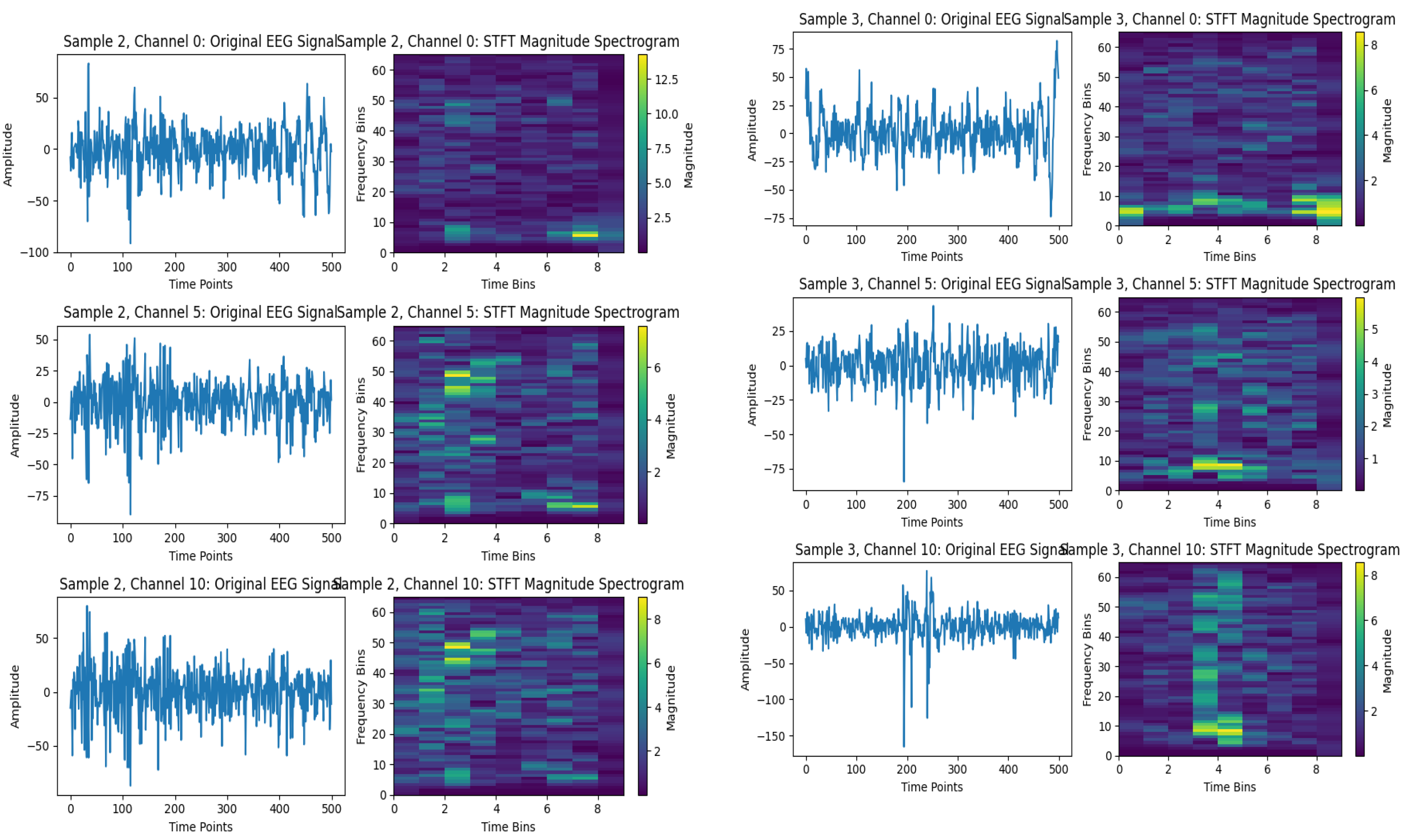
Figure 6.
Spectrograms of EEG Channels 5 and 10 for Subject 2 and Subject 3: (a) before ACE pre-processing, (b) after ACE pre-processing.
Figure 6.
Spectrograms of EEG Channels 5 and 10 for Subject 2 and Subject 3: (a) before ACE pre-processing, (b) after ACE pre-processing.
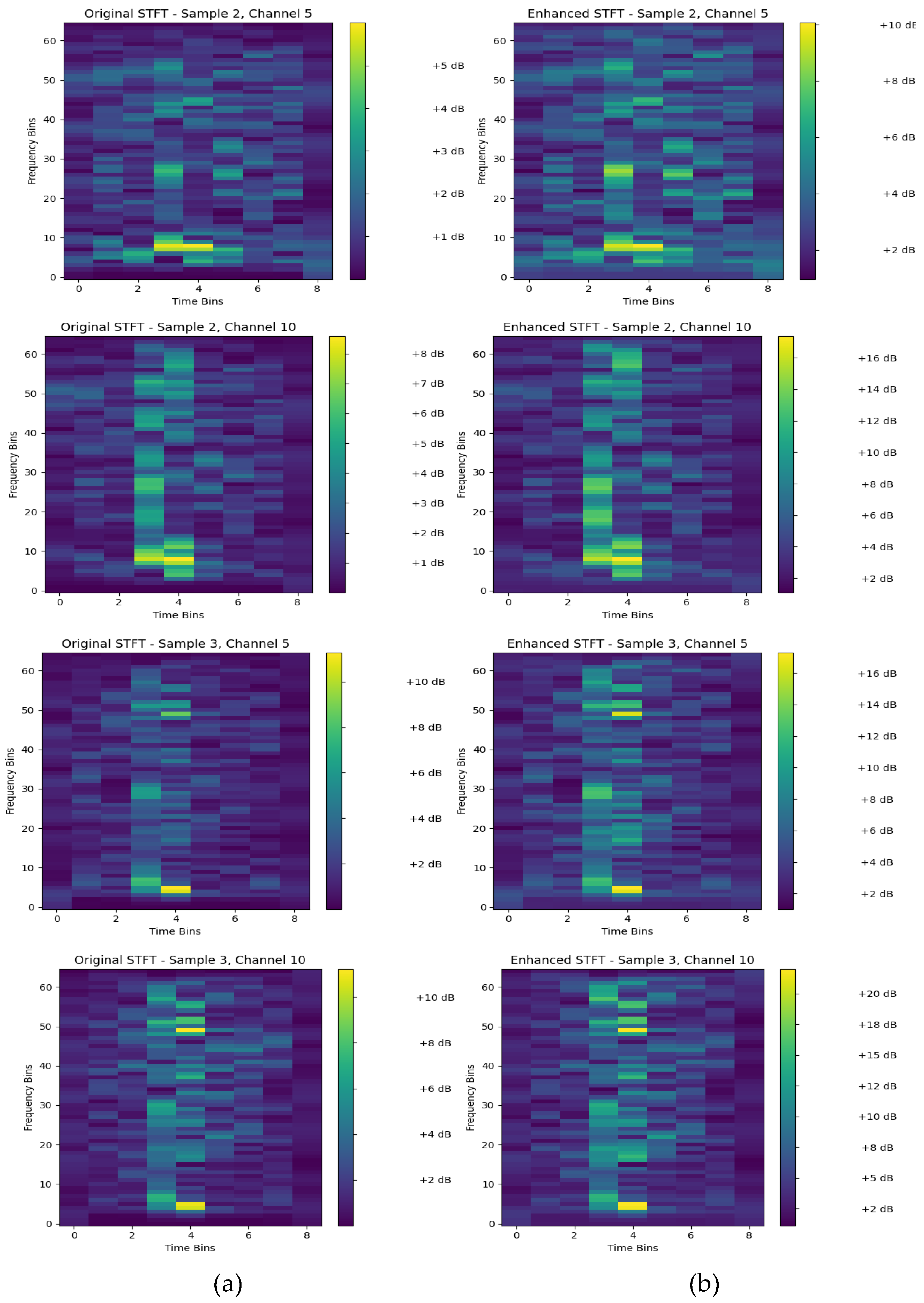
Figure 7.
Accuracy comparison between the original EEG (black), STFT feature extraction (orange), and the proposed STFT with ACE (green) across 42 subjects in the EAV dataset, demonstrating superior performance of the proposed method approach.
Figure 7.
Accuracy comparison between the original EEG (black), STFT feature extraction (orange), and the proposed STFT with ACE (green) across 42 subjects in the EAV dataset, demonstrating superior performance of the proposed method approach.
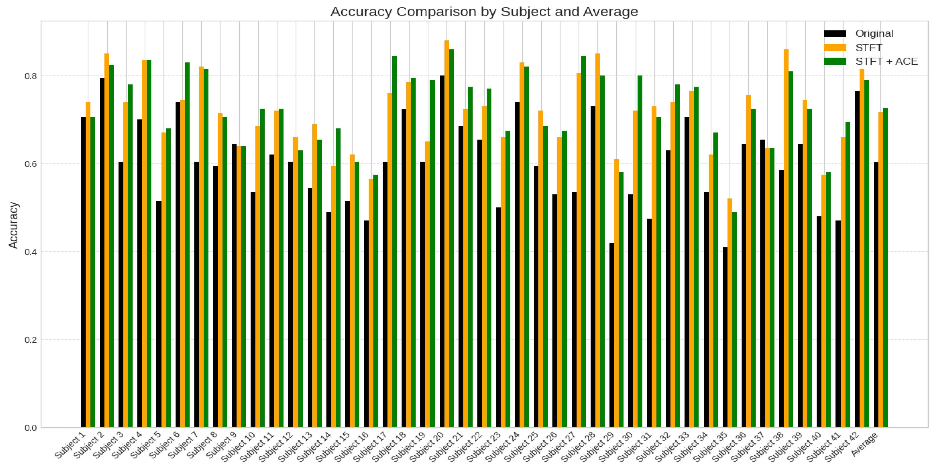
Figure 8.
F1-Score comparison between the original EEG (black), STFT feature extraction (orange), and the proposed STFT with ACE (green) across 42 subjects in the EAV dataset, demonstrating superior performance of the proposed method.
Figure 8.
F1-Score comparison between the original EEG (black), STFT feature extraction (orange), and the proposed STFT with ACE (green) across 42 subjects in the EAV dataset, demonstrating superior performance of the proposed method.
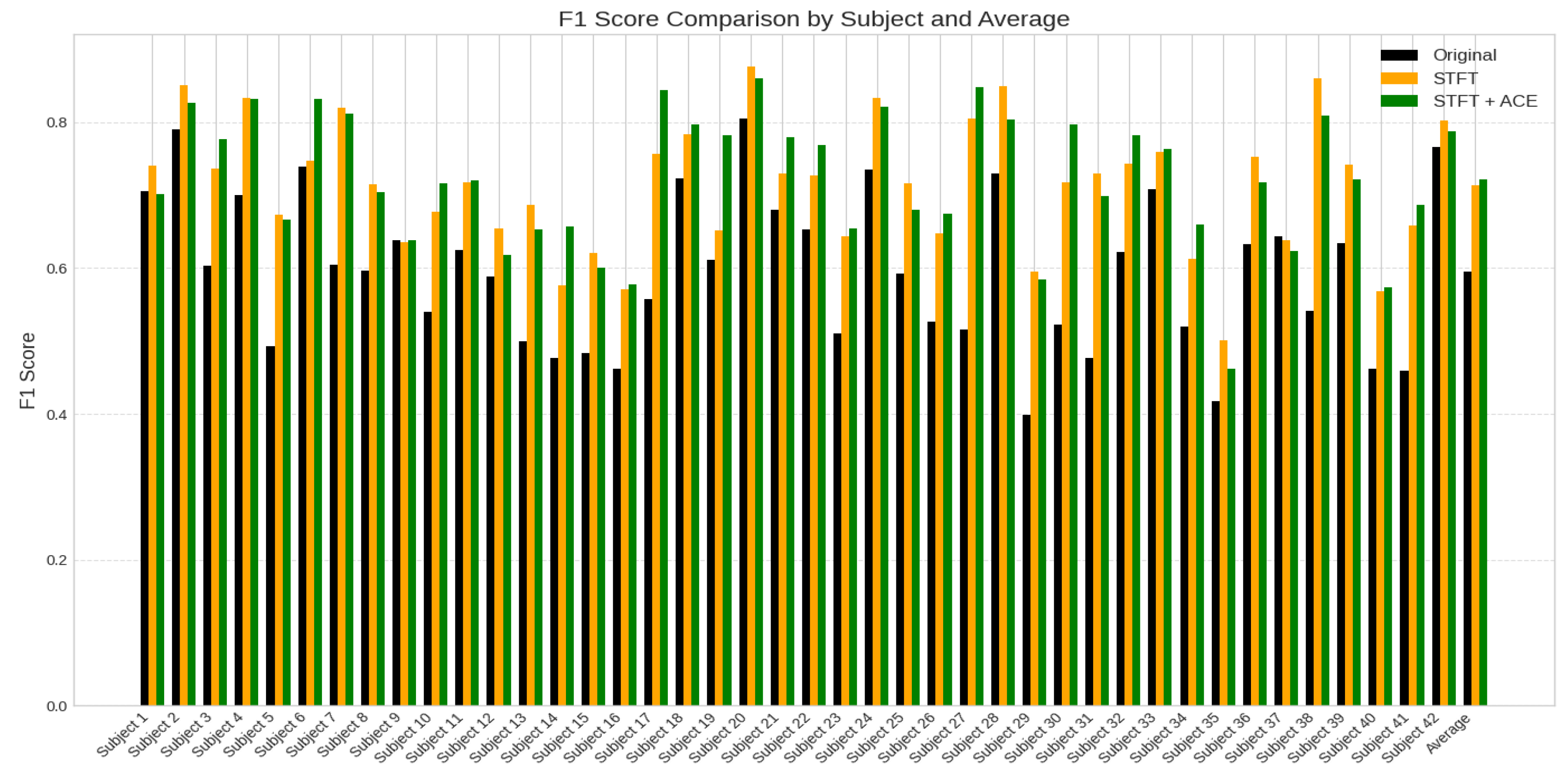
Figure 9.
The confusion matrix of the three experiments: (a) Original EEG dataset, (b) STFT for EEG dataset, (c) Enhanced STFT by ACE for the EEG dataset.
Figure 9.
The confusion matrix of the three experiments: (a) Original EEG dataset, (b) STFT for EEG dataset, (c) Enhanced STFT by ACE for the EEG dataset.
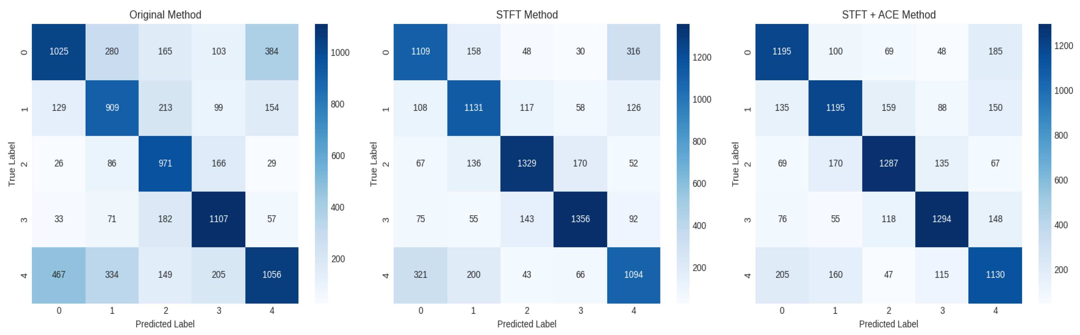
Figure 10.
The relationship between the number of ACE neighbors (N) and the model's accuracy.
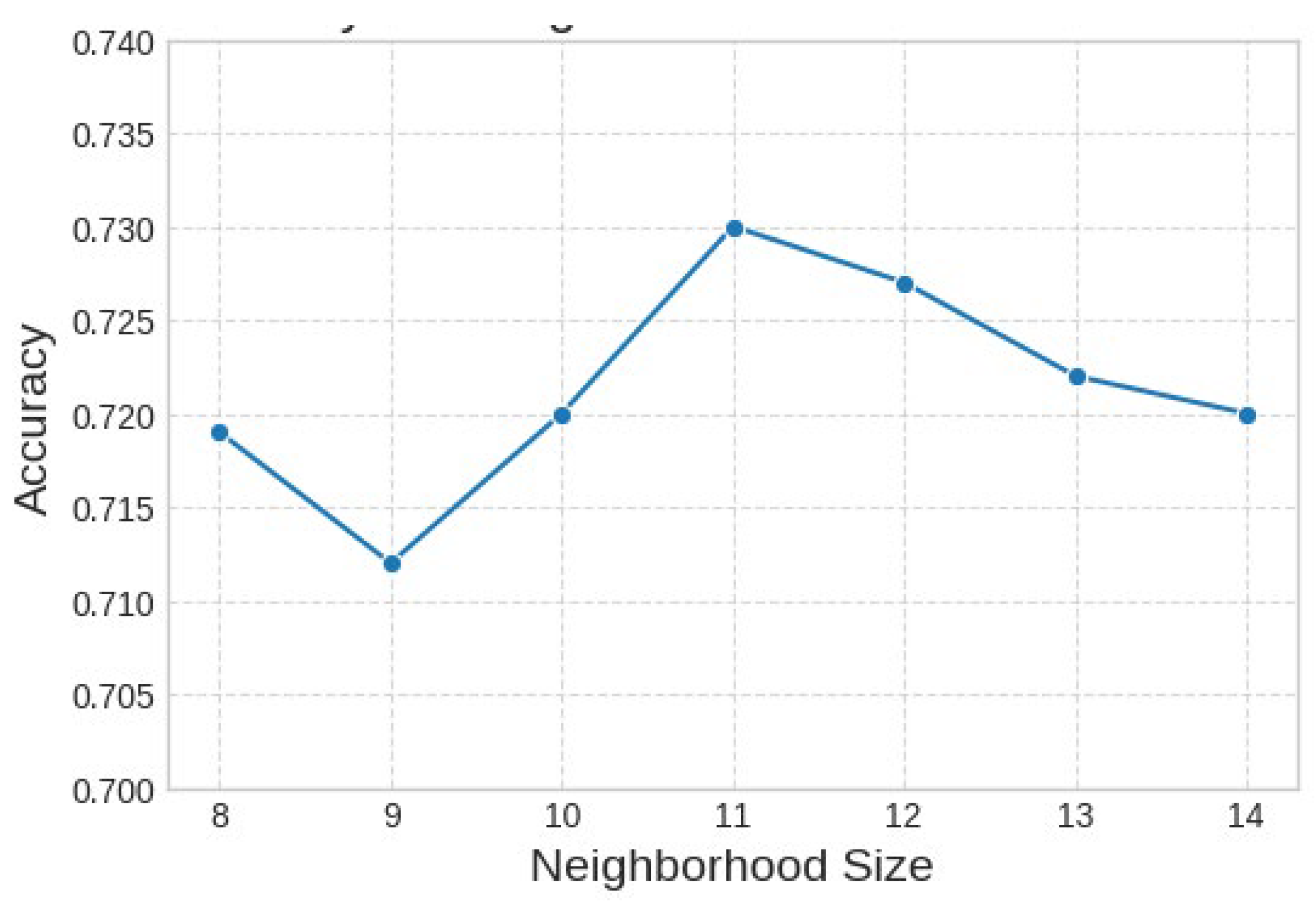
Figure 11.
EEG channel importance based on Mean Absolute SHAP values.
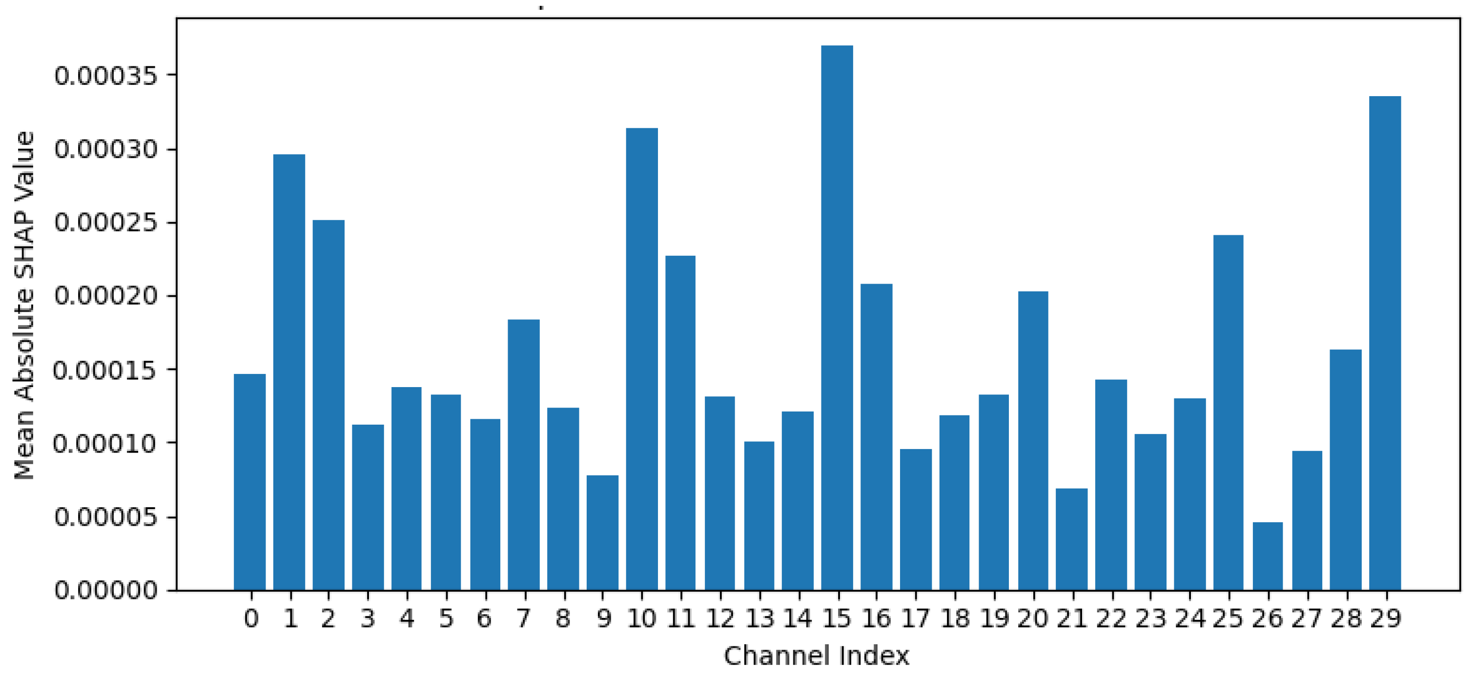

Table 1.
List CNN layers of the EEGnet.
| # | Layer name / Hyperparameters | No. | Layer name / Hyperparameters |
| 1 | Block 1: Input Tensor: | 8 | Block 2: SeparableConv2D: F2 filters, kernel (1, 8), padding = same |
| 2 | Conv2D: F1 filters, kernel (3, 3), padding = same | 9 | BatchNorm, ELU |
| 3 | BatchNorm | 10 | AveragePooling2D: (1, 2) |
| 4 | DepthwiseConv2D: kernel (C, 1), depth D, max-norm 1 | 11 | Dropout: δ |
| 5 | BatchNorm, ELU | 12 | Output:Flatten |
| 6 | AveragePooling2D: (1, 2) | 13 | Dense: Nclasses, max-norm η |
| 7 | Dropout: δ | 14 | Softmax Output: Class probabilities |
Table 2.
Confusion Matrix for Classification over two class labels.
| Input Class | Output Classes | |
| Class1 | Class 2 | |
| Class 1 | (TP) | (FN) |
| Class 2 | (FP) | (TN) |
Table 3.
Combined Accuracy of the classification experiment with 42 subjects: before STFT, after STFT and combined ACE with STFT.
Table 3.
Combined Accuracy of the classification experiment with 42 subjects: before STFT, after STFT and combined ACE with STFT.
| Experiment No. | Accuracy % EEGNet |
Accuracy % STFT + EEGNet |
Accuracy % Adaptive Contrast Enhancement (ACE) + STFT + EEGNet |
| 1 | 60.12 | 70.70 | 72.75 |
| 2 | 59.58 | 71.55 | 72.42 |
| 3 | 60.22 | 70.48 | 72.51 |
| 4 | 59.79 | 71.31 | 73.11 |
| 5 | 60.10 | 70.92 | 72.41 |
| 6 | 60.17 | 69.92 | 72.56 |
| 7 | 59.20 | 70.20 | 71.56 |
| 8 | 60.30 | 71.65 | 72.63 |
| Average | 59.94 | 70.84 | 72.50 |
Table 4.
The Confusion matrix for classification with STFT+ACE for the EEG dataset.
| Classes | 1 | 2 | 3 | 4 | 5 |
| 1 | 1195 | 100 | 69 | 48 | 185 |
| 2 | 135 | 1195 | 159 | 88 | 150 |
| 3 | 69 | 170 | 1287 | 135 | 67 |
| 4 | 76 | 55 | 118 | 1294 | 148 |
| 5 | 205 | 160 | 47 | 115 | 1130 |
| 42 subjects | 1680 | 1680 | 1680 | 1680 | 1680 |
| 1 subject | 40 | 40 | 40 | 40 | 40 |
| Class Acc. | 71.1% | 71.1% | 76.6% | 77.0% | 67.2% |
Disclaimer/Publisher’s Note: The statements, opinions and data contained in all publications are solely those of the individual author(s) and contributor(s) and not of MDPI and/or the editor(s). MDPI and/or the editor(s) disclaim responsibility for any injury to people or property resulting from any ideas, methods, instructions or products referred to in the content. |
© 2025 by the authors. Licensee MDPI, Basel, Switzerland. This article is an open access article distributed under the terms and conditions of the Creative Commons Attribution (CC BY) license (http://creativecommons.org/licenses/by/4.0/).
Copyright: This open access article is published under a Creative Commons CC BY 4.0 license, which permit the free download, distribution, and reuse, provided that the author and preprint are cited in any reuse.


