SIFT‐Based Automated Registration of Chandrayaan‐2 IIRS Hyperspectral Images

1. Introduction

Chandrayaan-2 has been orbiting the Moon since its launch in 2019. The Imaging Infra-Red Spectrometer (IIRS) on-board Chandrayaan-2 captures high-resolution images of the lunar surface with its 250 contiguous spectral bands in the wavelength range of 0.8 to 5.0 µm at a high spatial resolution of 80 m/pixel and a spectral resolution of ~20-25 nm [1], [2], [3], [4]. Data from IIRS is archived in the PDS4 format at ISRO’s PRADAN online portal (https://pradan.issdc.gov.in). IIRS was specifically designed to capture the hydration signature (observed at ~3 µm), in addition to using it to conduct high-resolution mineralogical analysis of the lunar surface. Till date, several techniques have been applied on IIRS data to process and analyze it, such as, automated geometric correction [2], photometric correction and analysis [3], and thermal correction and analysis [4]. A recent study highlights the applicability of using IIRS data to derive lunar surface temperatures at a high spatial resolution [5].

Before performing any scientific analysis using raster data, an accurate registration to its actual ground coordinates is necessary. As such, pixel-wise geometric information (including datum and map projection) is essential to accurately register a raster image. In the case of IIRS, its metadata provides latitude, longitude, scan and pixel numbers at a 50-pixel interval. [2] have utilized this metadata to create a tool to automate the complicated and time-taking process of seleno-referencing an IIRS image. However, we have observed that the metadata does not provide accurate pixel-to-pixel coordinate information, and its usage results in an error/offset of the seleno-referenced IIRS image. An alternative way to seleno-reference IIRS strips could be the manual extraction of the GCPs and performing an image-to-image seleno-referencing with LRO-WAC (Lunar Reconnaissance Orbiter - Wide Angle Camera) data (spatial resolution of 100 m). However, manually seleno-referencing an IIRS image is a tedious and time-consuming process which is prone to errors/offsets of several meters. Therefore, there is a dire need for a robust method that can accurately seleno-reference IIRS images quickly, reliably, and accurately. Hence, the primary motivation of this study is to develop and implement an automated seleno-referencing pipeline that is capable of overcoming the limitations of the derived geometry as well as providing a fast and user-friendly way to precisely seleno-reference IIRS images. The subsequent sections provide a detailed account of the methodology that has been developed in this study for an automated, feature-based seleno-referencing of IIRS strips via the Scale-Invariant Feature Transform (SIFT) algorithm.

2. Data and Methods

A. Chandrayaan-2 IIRS level-1 data

The input data consists of IIRS level-1 calibrated radiance products typically provided in the PDS4-compliant QUB format, which is a Band-Sequential (BSQ) multi-band image. This data represents the calibrated radiance values acquired by IIRS. Accompanying each QUB file is an XML metadata file, which contains supporting information like image corner coordinates, which have been used in our algorithm.

B. LRO-WAC global mosaic

The basemap employed for reference in this study is the LRO-WAC global lunar mosaic. This is a publicly available seleno-referenced dataset, provided in GeoTIFF format. For our purpose, the LRO-WAC mosaic serves as the geometric reference standard. The specific Coordinate Reference System (CRS) of the WAC mosaic (i.e., Simple Cylindrical Moon) is extracted directly from the file and used as the target CRS for the seleno-referenced IIRS output.

The core objective of this study is to achieve a significantly high geometric accuracy by directly registering the IIRS image to the corresponding LRO-WAC image using the image-to-image feature-matching technique. It is hypothesized that this feature-based registration will effectively compensate for the accumulated errors in spacecraft pointing, orbit, and sensor modelling, yielding a seleno-referenced IIRS product that exhibits a substantially improved spatial alignment with the LRO-WAC standard.

C. Region of Interest (ROI) definition and pre-processing

A single band is selected from the IIRS hyperspectral data cube for processing. In this case, an ideal band should have a good signal-to-noise ratio (SNR) and surface features that are easily visible. Moreover, the IIRS level-1 datasets have an incorrect spatial orientation of the image array relative to the seleno-graphic area it represents, as defined by the metadata. Prior to feature-matching against the WAC mosaic, the algorithm performs an orientation-check on the IIRS strips using the XML metadata. Wherever necessary, an IIRS strip automatically undergoes an orientation correction, such that misalignments, if any, could be identified and removed by the algorithm.

The extracted IIRS seleno-graphic corner coordinates (longitude and latitude) are then used to extract the pixel coordinates of the corresponding WAC ROI pixel coordinates (column, row). Further, a minimum bounding box (in WAC pixel coordinates) is determined that encompasses all transformed IIRS corners. Padding is then applied to this bounding box, to ensure that the extracted WAC region sufficiently overlaps the IIRS strip. Then, the padded pixel coordinates are clipped to the valid dimensions of the WAC mosaic (0 to RasterXSize-1, 0 to RasterYSize-1) to prevent out-of-bounds requests. The final ROI is defined as a tuple ($y_{min\_final}$, $y_{\mathrm{m}\mathrm{a}\mathrm{x}\_final}$, $x_{\mathrm{m}\mathrm{i}\mathrm{n}\_final}$, $x_{\mathrm{m}\mathrm{a}\mathrm{x}\_final}$) representing the rows and columns to extract from the WAC mosaic.

Both the IIRS band array and the extracted WAC ROI array are divided into smaller, overlapping square patches or tiles. A grid size and an overlap percentage are defined. The coordinates ($x_{min}$, $y_{min}$, $x_{max}$, $y_{max}$) for each tile within its respective full array (rescaled IIRS or WAC ROI) are stored. Tiles < 1/2(grid size) are discarded.

Each IIRS and WAC patch is individually normalized. Invalid pixels are masked out. The 2^nd and 98^th percentiles of the valid pixel values are calculated. These percentiles define the robust minimum ($p_{low}$) and maximum ($p_{high}$) intensity range, mitigating the effects of extreme outliers. Valid pixels are then clipped to this range and then linearly scaled to the floating-point range [0.0, 1.0] using the following equation:

$$\mathit{n}\mathit{o}\mathit{r}\mathit{m}=\left({\displaystyle \frac{(\mathit{c}\mathit{l}\mathit{i}\mathit{p}\mathit{p}\mathit{e}{\mathit{d}}_{\mathit{v}\mathit{a}\mathit{l}\mathit{u}\mathit{e}}-{\mathit{p}}_{\mathit{l}\mathit{o}\mathit{w}})}{{\mathit{p}}_{\mathit{h}\mathit{i}\mathit{g}\mathit{h}}-{\mathit{p}}_{\mathit{l}\mathit{o}\mathit{w}}+\mathit{e}\mathit{p}\mathit{s}\mathit{i}\mathit{l}\mathit{o}\mathit{n}}}\right)$$

(1)

The means and standard deviations of these 0-1 normalized valid pixels are calculated and stored along with the percentile values (stats). Patches with insufficient valid pixels or near-constant values (low percentile range) are skipped.

The initially normalized IIRS patch (in its 0-1 float representation) is adjusted to match the statistics of the normalized WAC patch. Using the calculated means (${mean}_{IIRS}$, ${mean}_{WAC}$) and standard deviations (${std}_{IIRS}$, ${std}_{WAC}$) from the initial normalization step, the value of each valid normalized IIRS pixel ($p_{IIRSnorm}$) is adjusted using the following equation:

$${\mathit{p}}_{\mathit{I}\mathit{I}\mathit{R}\mathit{S}\_\mathit{a}\mathit{d}\mathit{j}\mathit{u}\mathit{s}\mathit{t}\mathit{e}\mathit{d}}={\mathit{m}\mathit{e}\mathit{a}\mathit{n}}_{\mathit{W}\mathit{A}\mathit{C}}+({\mathit{p}}_{\mathit{I}\mathit{I}\mathit{R}\mathit{S}\_\mathit{n}\mathit{o}\mathit{r}\mathit{m}}-{\mathit{m}\mathit{e}\mathit{a}\mathit{n}}_{\mathit{I}\mathit{I}\mathit{R}\mathit{S}})\times \left({\displaystyle \frac{\mathit{s}\mathit{t}{\mathit{d}}_{\mathit{W}\mathit{A}\mathit{C}}}{\mathit{s}\mathit{t}{\mathit{d}}_{\mathit{I}\mathit{I}\mathit{R}\mathit{S}}}}\right)$$

(2)

If ${std}_{WAC}$ of the IIRS patch ~ 0, the adjustment is skipped, and the IIRS patch that was initially normalized is used.

Both the potentially adjusted and normalized IIRS float patch and the normalized WAC float patch are clipped to the [0.0, 1.0] range and then scaled to [0, 255], converting them to the uint8 format, suitable for many OpenCV feature detectors.

D. The Scale-Invariant Feature Transform (SIFT) algorithm for automated feature-matching

The SIFT algorithm is selected as the primary feature detection and matching algorithm due to its demonstrated robustness in prominent computer vision and remote sensing applications [6], [7]. SIFT’s particular invariance to scale, rotation, and illumination changes makes it suitable for matching features between hyperspectral imagery acquired under varying geometric and illumination conditions. Thus, the algorithm’s ability to detect distinctive features across different spatial resolutions is crucial for this application, given the resolution difference between IIRS and LRO-WAC datasets.

Previous studies, such as, [8], have demonstrated SIFT’s effectiveness in planetary surface feature-matching applications, particularly for lunar terrain where traditional correlation-based methods often fail due to the uniform albedo and subtle topographic variations of the lunar surface. The multi-scale nature of SIFT detection ensures a robust feature identification across the scale differences inherent in multi-sensor lunar datasets [7].

The implementation employs SIFT’s standard two-stage approach – the initial keypoint detection followed by descriptor computation. Keypoint detection identifies candidate interest points based on scale-space extrema using the Difference of Gaussians (DoG) approach across multiple octaves. The descriptor computation stage calculates 128-dimensional feature vectors for each detected keypoint, potentially refining the keypoint locations and rejecting unstable features. This separation enables the differentiation between detection failures (insufficient features in the imagery) and descriptor computation failures (unstable feature characteristics), facilitating quality assessment and troubleshooting.

Feature correspondence is established using a brute-force matcher with L2 norm and k-nearest neighbour search (k=2) to enable ratio testing for ambiguous match filtering. A Lowe’s ratio test with a 0.75 threshold retains matches only when the nearest-neighbour distance is less than 75% of the second nearest neighbour distance, effectively removing correspondences in repetitive lunar terrain patterns like crater fields. Also, a geometric verification using a RANSAC-based homography estimation is done, which requires a minimum of 8-point correspondences with a 3.0-pixel re-projection threshold to account for sensor resolution and terrain characteristics [8].

Additionally, the homography quality is assessed to reject degenerate transformations that indicate false correspondences or inappropriate geometric models. This multi-stage filtering approach ensures a robust feature-matching despite the challenging visual characteristics of lunar surface imagery.

SIFT-derived correspondences serve as the foundation for GCP generation. The robustness of the SIFT matching process directly impacts the overall seleno-referencing quality, as the spatial distribution and accuracy of the extracted GCPs determine the fidelity of the final geometric correction applied to IIRS hyperspectral data.

For a given IIRS tile, the WAC tile that yields the highest number of inliers after the filtering steps is considered as the "best-match." If a best match with inliers > 0 is found for an IIRS tile, for each inlier match in the IIRS source coordinate, we get the keypoint location ($x_{patch}$, $y_{patch}$) within the rescaled IIRS tile. We then add the tile’s top-left offset to get the coordinate ($x_{rescaled}$, $y_{rescaled}$) within the fully rescaled IIRS array. Subsequently, we invert the initial flip operations. In the case of LRO-WAC, for each inlier match in the WAC target coordinate, we obtain keypoint locations $x_{patchWAC}$, $y_{patchWAC}$ within the WAC tile, then add the WAC tile’s top-left offset within the ROI to get the coordinate within the extracted WAC ROI array. Then, we store the pair ($x_{orig}$, $y_{orig}$, longitude, latitude) as a potential GCP.

E. Output

All the generated GCPs ($x_{orig}$, $y_{orig}$, longitude, latitude) from the successful tile matches are aggregated into a list. This list is written to a CSV file in the output directory. The CSV file contains the header ($x_{pixel}$, $y_{pixel}$, longitude, latitude) matching the format expected by the subsequent seleno-referencing script.

F. Georeferencing transformation

A minimum distance of 15-20 pixels is specified, which acts as a filter to ensure a more even spatial distribution of the GCPs across the IIRS image extent. The minimum and maximum ($x_{pixel}$ and $y_{pixel}$) coordinates are determined from the input GCPs. A grid is conceptually overlaid on the IIRS pixel-space, with cell sizes equal to minimum distance. For each grid cell containing one or more GCPs, the Euclidean distance of each point within the cell to the cell’s centre is calculated. Only the GCP closest to the centre of each occupied cell is retained. This effectively removes the clustered points while preserving spatial coverage.

Then we establish the number of GCPs that are available for each image. We then apply the condition: ${\mathit{filter}}_{\mathit{outliers}}=\mathit{True}$ and check if a sufficient number of GCPs are available (> 20). This statistical filter is then applied to remove those points that deviate significantly from the general geometric trend. The Euclidean distance (residual error) between the actual target coordinates and the predicted target coordinates are calculated for each GCP. The means and the standard deviations of these residual errors are then computed. The Z-score for each GCP’s residual error is also calculated from (3), such that:

$$\mathit{Z}=\left({\displaystyle \frac{\mathit{e}\mathit{r}\mathit{r}\mathit{o}\mathit{r}-\mathit{m}\mathit{e}\mathit{a}{\mathit{n}}_{\mathit{e}\mathit{r}\mathit{r}\mathit{o}\mathit{r}}}{\mathit{s}\mathit{t}{\mathit{d}}_{\mathit{e}\mathit{r}\mathit{r}\mathit{o}\mathit{r}}}}\right)$$

(3)

GCPs with a Z-score exceeding a defined threshold are considered as outliers and are removed from the list. A geometric transformation model, such as a polynomial, is selected for warping. Higher-order polynomials can model more complex distortions but require more well-distributed GCPs, which risk overfitting.

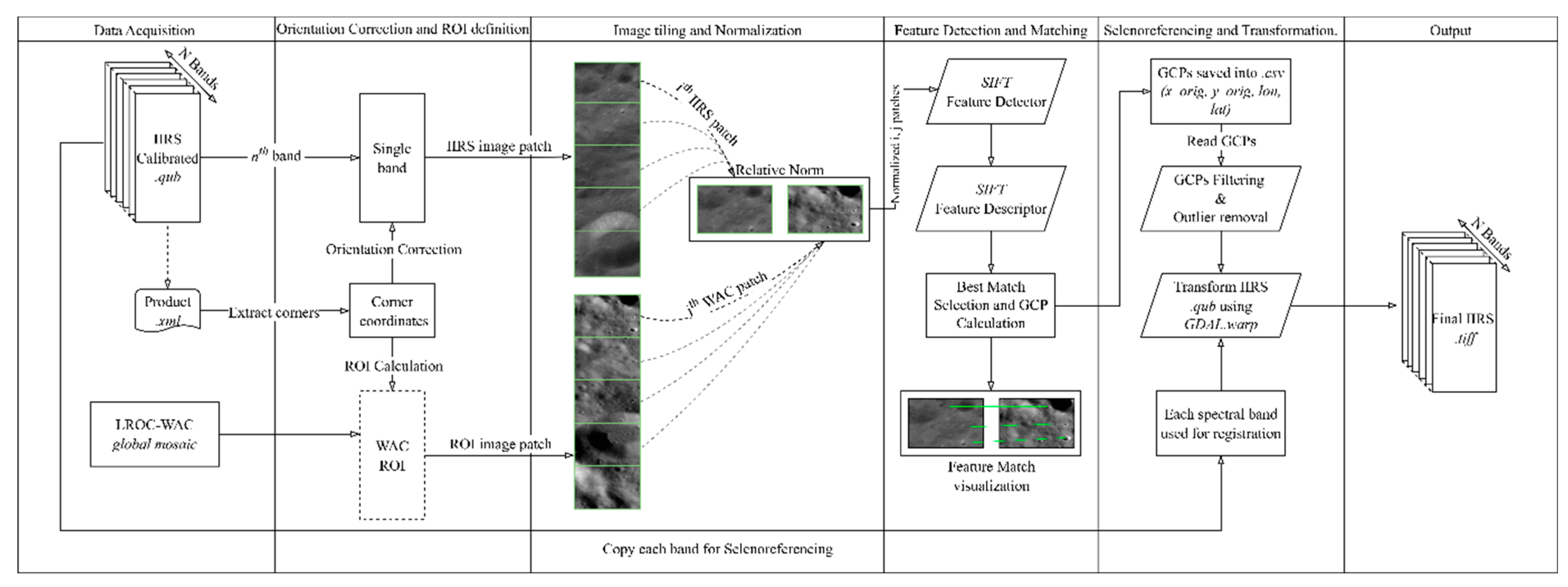
The gdal.warp operation creates the final georeferenced GeoTIFF file directly. The final output file contains the IIRS data warped to the WAC mosaic’s CRS at the spatial resolution of IIRS. Using the algorithm described above, the time required to process a single IIRS strip can vary between ~two to ~five minutes, depending on the length of the strip. Additionally, the output generates a GeoTIFF image containing 250 hyperspectral bands. The methodology described to implement the seleno-referencing process has been summarized in a flowchart (Figure 1).

Figure 1. A flowchart depicting the methodology applied to seleno-reference an IIRS image using the SIFT algorithm.

Figure 1. A flowchart depicting the methodology applied to seleno-reference an IIRS image using the SIFT algorithm.

G. Validation

After the application of the steps mentioned above, the resultant seleno-referenced IIRS GeoTIFF file is overlaid onto the LRO-WAC mosaic within a GIS environment. A careful visual inspection of the spatial alignment of prominent, unambiguous features such as crater rims, central peaks, rilles, and ridges across the entire extent of the IIRS strip is carried out. Care is taken to check for any systematic offsets, rotations, or local distortions.

A set of well-defined Independent Check Points (ICPs) that are clearly visible and precisely locatable are manually identified in both the original IIRS image and the WAC mosaic. A good distribution of ICPs across the IIRS strip is crucial.

3. Results and Discussion

A total of ~200 IIRS strips were processed using a SIFT-based algorithm, which is described in Section II (E). The large pool of IIRS strips allowed us to create a database using which we were able to quantitatively assess the accuracy of the seleno-referenced dataset and estimate the associated errors. Our analysis of the processed IIRS dataset reveals that the algorithm has worked well on the IIRS images and has taken care of the different solar incidence angles that each IIRS strip possesses. We chose only those IIRS strips whose acquisition times ranged between the lunar sunrise (~07:00 hours local lunar time) and the lunar sunset (~19:00 hours local lunar time), as well as between the latitudes of ±55°. The 12-hour time-window has allowed us to analyze IIRS strips across different times of a lunar day and assess whether the time of acquisition (and consequently, the solar incidence angles) has any impact on the performance of the algorithm.

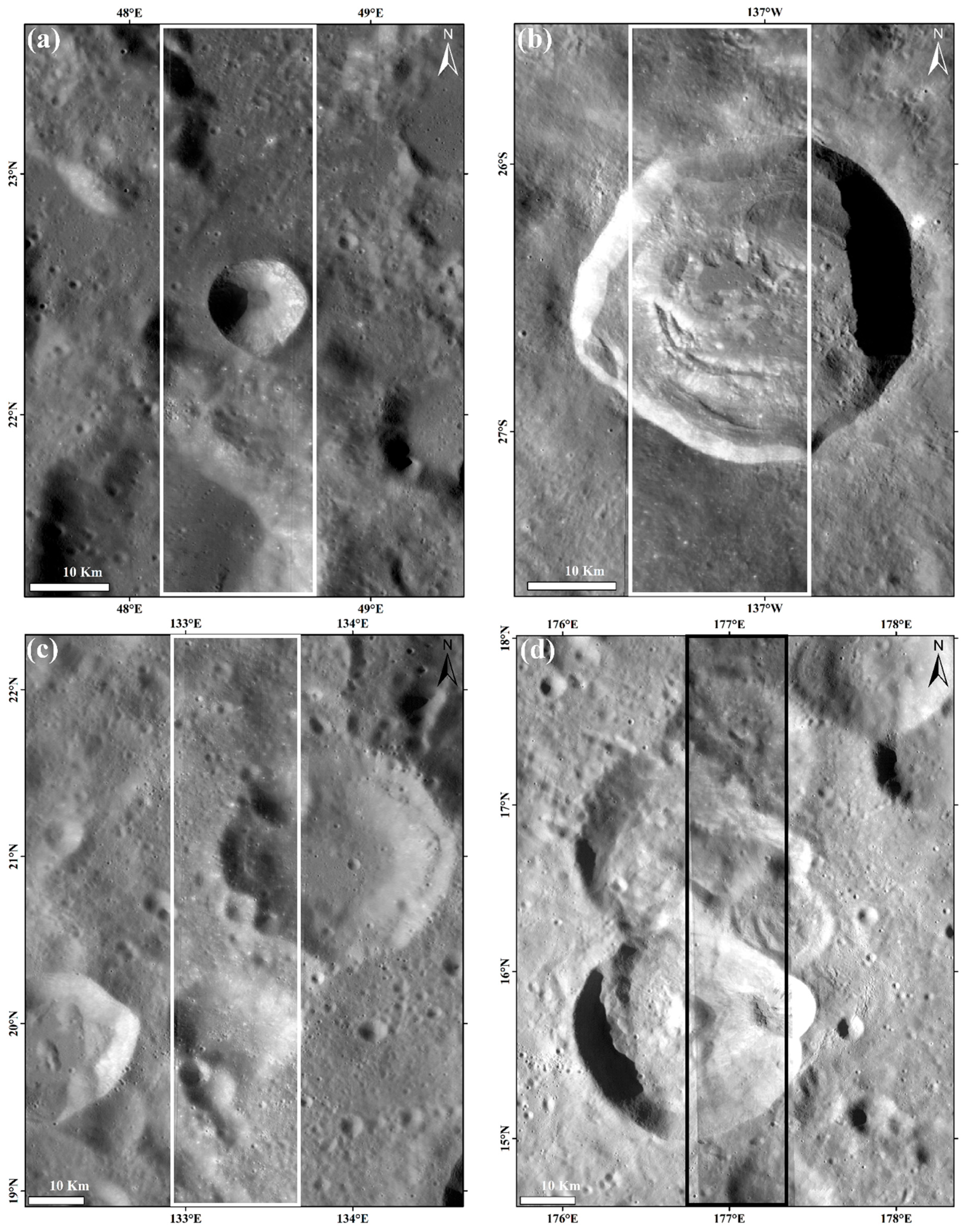
Figure 2 shows an example of a sample of four separate and processed IIRS strips that pass primarily over the lunar maria (a-d). RMS errors (RMSE_total) calculated (in metres) for each strip have been shown in Table 1. The estimated RMS errors for the strips passing over the maria range between ~67.5 m to ~82.5 m, indicating that for three of the strips (Figure 2 a, b, d), the RMS errors are within the resolution of a single IIRS pixel (~80 m), which further highlights the efficacy of the algorithm. Similarly, Figure 3 shows four processed IIRS strips that pass primarily over parts of the lunar highlands (a-d). For the highlands example, the estimated RMS errors were found to range between ~64 m to 66.6 m, two of which are from those IIRS strips which are less than the resolution of a single IIRS pixel (a, b), while the other two (c, d) have values such as 83.6 m and 84.5 m, respectively (Table 1). The mean RMS error for the eight strips (~73 m) was also found to be below the resolution of an IIRS pixel. The details regarding the RMS errors estimated for the eight IIRS strips are provided in Table 1 and Figure 4.

A specific cause that could be attributed to the range of the measured RMS errors could not be found. However, one possible cause seems to be more relevant than the other possible causes – a difference in the solar incidence angles. The LRO-WAC dataset (which has been used a reference image in this study) has a range of solar incidence angles (between 48°-72° at the equator) [10], which are relatively higher than IIRS and hence, generally do not match the IIRS values (~20° to ~43° between the latitudes of 5° S to 28° N). It is important to note that IIRS essentially has comparatively lower incidence angles across most of the ~200 strips that we have analyzed in this study. Consequently, based on our analysis, it was found that the differences create potential conditions for misidentification of the features on the lunar surface for the SIFT algorithm. Such occurrences could lead to an error equivalent to approximately one IIRS pixel (60 m < error < 90 m) near the equator, potentially increasing to up to three IIRS pixels (240 m < error < 300 m) upwards of ±40° latitude. However, in spite of the large differences in the incidence angles of IIRS and WAC, the SIFT algorithm is able to identify surface features from WAC and match them accurately for a majority of the IIRS images.

Figure 2. Four examples of IIRS strips seleno-referenced using the SIFT algorithm. (a) to (d) show the IIRS strips that are from the lunar maria. Extents of the IIRS strips are indicated by white rectangles. Basemap is LRO-WAC. For the corresponding IIRS strip IDs (a-d), please refer to Table 1.

Figure 2. Four examples of IIRS strips seleno-referenced using the SIFT algorithm. (a) to (d) show the IIRS strips that are from the lunar maria. Extents of the IIRS strips are indicated by white rectangles. Basemap is LRO-WAC. For the corresponding IIRS strip IDs (a-d), please refer to Table 1.

Figure 3. Four examples of IIRS strips seleno-referenced using the SIFT algorithm. (a) to (d) show the IIRS strips that are from the lunar highlands. Extents of the IIRS strips are shown in white for (a-c), and in black for (d). Basemap is LRO-WAC. For the corresponding IIRS strip IDs, please refer to Table 1.

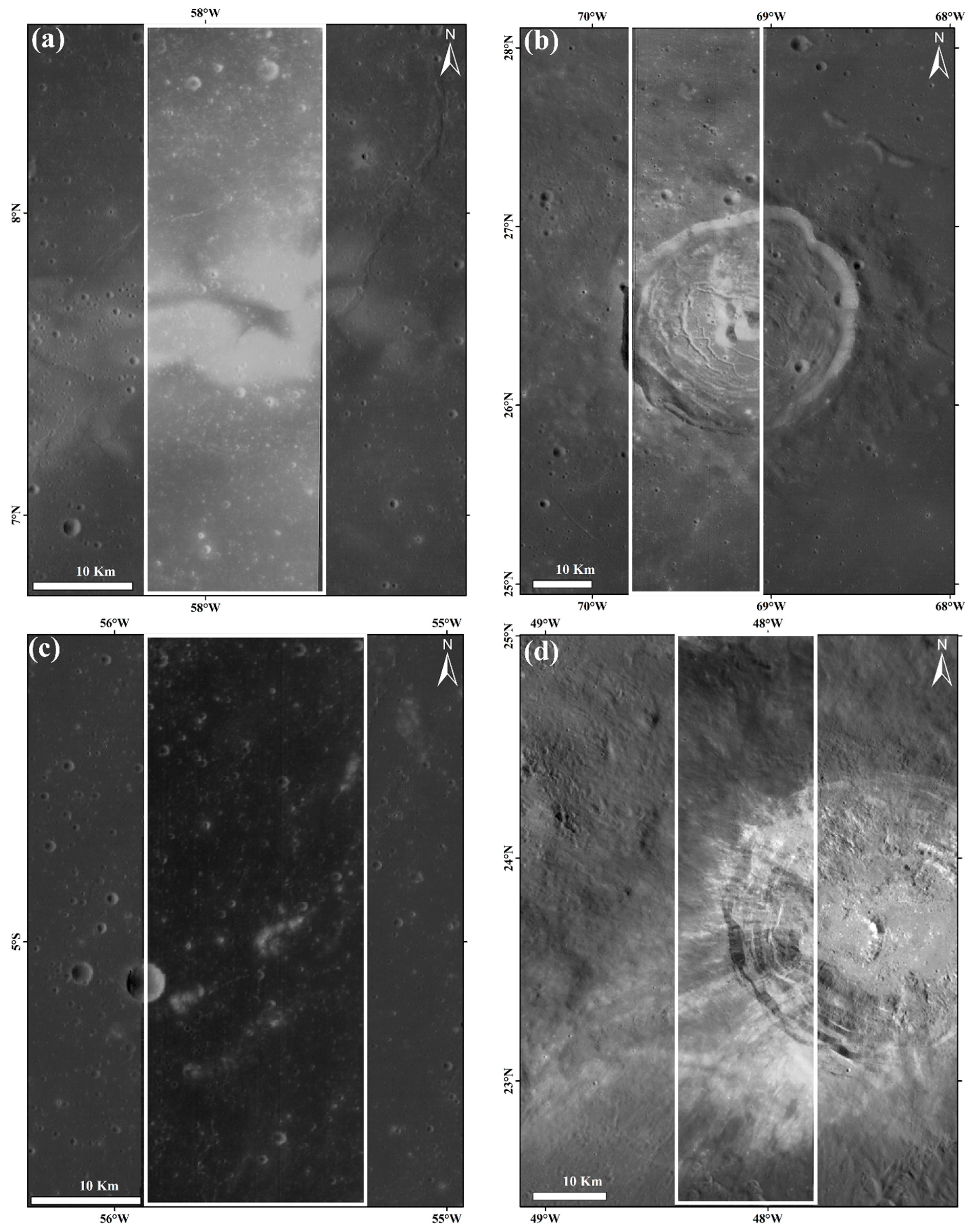
Figure 3. Four examples of IIRS strips seleno-referenced using the SIFT algorithm. (a) to (d) show the IIRS strips that are from the lunar highlands. Extents of the IIRS strips are shown in white for (a-c), and in black for (d). Basemap is LRO-WAC. For the corresponding IIRS strip IDs, please refer to Table 1.

In order to understand whether latitude plays a role in the seleno-referencing process, three separate IIRS strips were scrutinized in detail (Figure 5). One of the images (CH2_IIR_NCI_20240201T1026227387_D_IMG_D18) extends from ~60° S up to 20° S. RMS errors have been computed at every few degrees in latitude along the extent of the image. The estimated RMSE values ranged between ~1,040 m at 60° S to ~70 m at 47° S and ~65 m at 22° S. This indicates that with increasing latitude (beyond ±55°), RMS errors increase exponentially. This is due to the fact that beyond ±55°, the curvature of the Moon tends to become more prominent, which affects the images captured by sensors like IIRS as well as those captured by LRO, and is therefore a limitation of this study. Similarly, the second image (CH2_IIR_NCI_20240422T1522156952_D_IMG_D18), which spans from 40° N up to 70° N, has similar RMSE values, such that at lower latitudes the value is less than IIRS’s spatial resolution, whereas at its maximum extent, it was found to be ~2,000 m. Therefore, it is evident that at higher latitudes (beyond ±55°), RMS errors are exceptionally higher as compared to the lower latitudes. The third image (CH2_IIR_NCI_20231117T1110268671_D_IMG_D18) extends from ~8° S to ~32° N. The corresponding RMS errors estimated from this image are <80 m for all instances. Hence, according to the values in Figure 5, it was found that latitude does play a role for the current seleno-referencing process which impacts the derived accuracy of the IIRS strips according to their latitudinal extents.

Figure 4. A plot of RMS errors computed from the eight IIRS strips as shown in Table 1. For IIRS figure IDs mentioned in the figure above, please refer to the ‘Remarks’ column in Table 1.

Figure 4. A plot of RMS errors computed from the eight IIRS strips as shown in Table 1. For IIRS figure IDs mentioned in the figure above, please refer to the ‘Remarks’ column in Table 1.

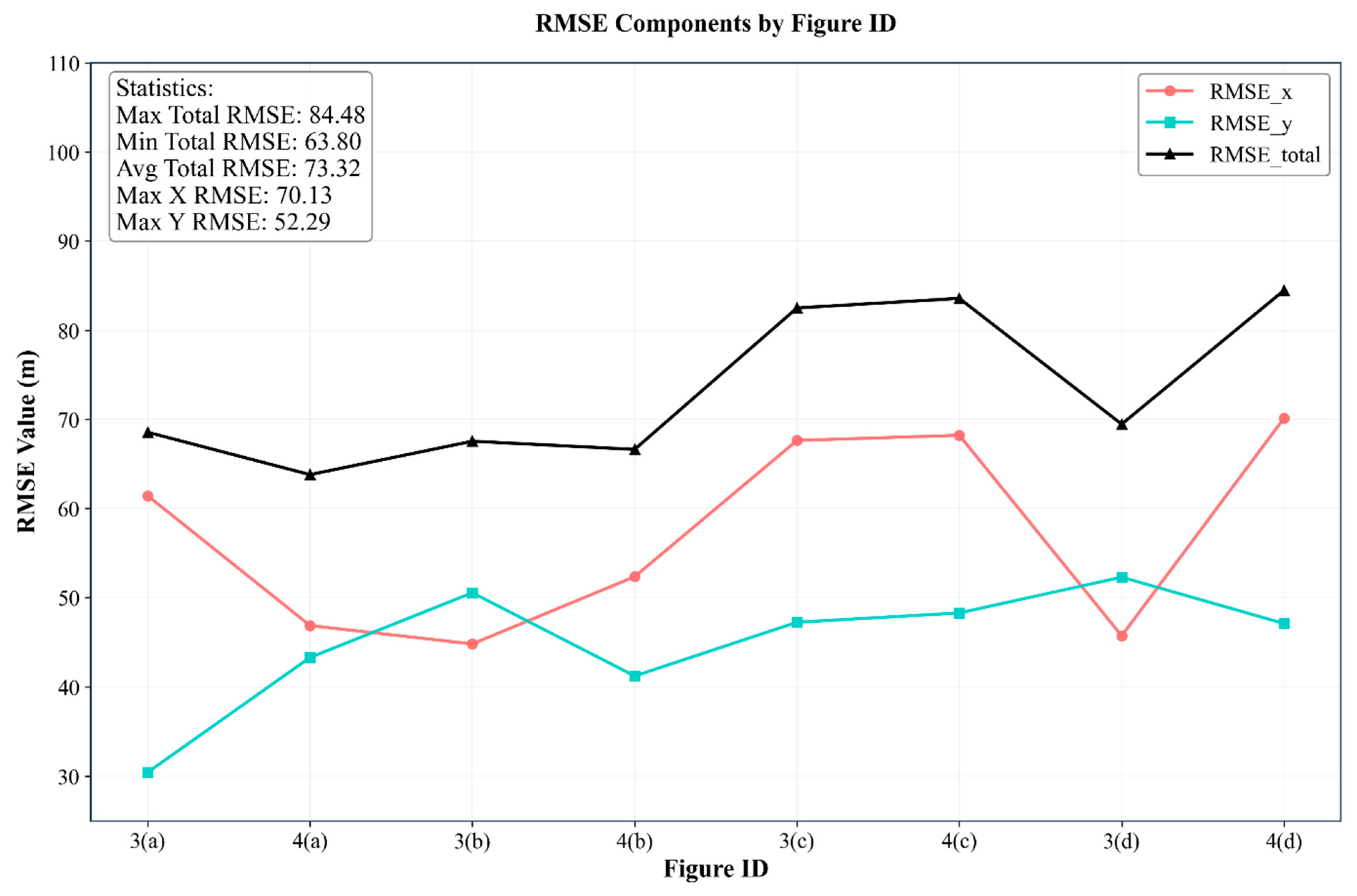
Figure 5. A plot of RMS errors plotted against different latitudes (60° S to 70° N) using three IIRS strips.

Figure 5. A plot of RMS errors plotted against different latitudes (60° S to 70° N) using three IIRS strips.

4. Conclusions

This study presents a methodology to automate the process of seleno-referencing IIRS images using LRO-WAC as a reference image. The SIFT algorithm, which has been used to automatically detect GCPs from both WAC and IIRS, is explained in detail in Section 2. Results from the study indicate that SIFT is able to both identify and match the derived GCPs from WAC and IIRS, using which IIRS strips have been seleno-referenced (Section 3). A sample of eight IIRS strips shows the efficacy of the SIFT algorithm, such that, the measured RMS errors were within the size of a single IIRS pixel for five of the eight IIRS strips (Table 1). For the remaining three strips, the RMS errors were less than ~85 m. The mean RMS error was calculated to be ~73 m. In addition, three IIRS strips were analyzed to find out whether latitude plays a role in the RMS errors estimated from IIRS strips. However, based on the results presented in Figure 5, a correlation was obtained between latitude and the derived RMSE values, which was seen to affect the accuracy of the seleno-referenced IIRS strips beyond ±55°, without significantly impacting the lower latitudes. Finally, the SIFT algorithm explained here could be used to automatically detect GCPs from an individual IIRS strip and accurately seleno-reference it as per the actual surface coordinates in a much faster (less than five minutes), more accurate and more reliably than the existing ways, i.e., either manually seleno-referencing them or by using the attached metadata provided with each IIRS strip. Additionally, this algorithm may also be used on similar unregistered planetary datasets, for which a standard reference map with a comparable spatial resolution is necessary.

References

- Chowdhury, A.R., Banerjee, A., Joshi, S.R., Dutta, M., Kumar, A., Bhattacharya, S., Amitabh, Rehman, S.U., Bhati, S., Karelia, J.C., Biswas, A., Saxena, A.R., Sharma, S., Somani, S.R., Bhagat, H.V., Sharma, J., Ghonia, D.N., Bokarwadia, B.B., Parasar, A., (2020). Imaging Infrared Spectrometer onboard Chandrayaan-2 Orbiter. Curr. Sci. 118, 368. [CrossRef]
- Ishan Rayal, P. Chauhan, P. K. Thakur, and U. Kumar, “Python-Based Open-Source Tool for Automating Seleno-Referencing of Chandrayaan-2 Hyper-Spectral Data Cubes,” Photonirvachak, vol. 52, no. 2, pp. 305–313, (2024). [CrossRef]
- S. Bose, A. Kumari, R. Biswas, Lala, and A. P. Krishna, “Photometric correction of images obtained from Chandrayaan-2 Imaging Infra-Red Spectrometer (IIRS) data,” Advances in Space Research, vol. 73, no. 5, pp. 2720–2752, (2023). [CrossRef]
- P. A. Verma, M. Chauhan, and P. Chauhan, “Lunar surface temperature estimation and thermal emission correction using Chandrayaan-2 imaging infrared spectrometer data for H2O & OH detection using 3 μm hydration feature,” Icarus, vol. 383, p. 115075, (2022). [CrossRef]
- Bose, S., Karunakaran, D., Kapadia, T., Panwar, N., Chandane, A. & Srivastava, N. (2025). Daytime surface temperatures of the Moon derived from high-resolution IIRS on-board Chandrayaan-2; Manuscript under revision.
- D. G. Lowe, “Distinctive Image Features from Scale-Invariant Keypoints,” International Journal of Computer Vision, vol. 60, no. 2, pp. 91–110, (2004). [CrossRef]
- W. Ma et al., “Remote Sensing Image Registration with Modified SIFT and Enhanced Feature Matching,” vol. 14, no. 1, pp. 3–7, (2017). [CrossRef]
- B. Wu, H. Zeng, and H. Hu, “Illumination invariant feature point matching for high-resolution planetary remote sensing images,” Planetary and Space Science, vol. 152, pp. 45–54, (2018). [CrossRef]
- Fischler, M. A., & Bolles, R. C. (1981). Random sample consensus: a paradigm for model fitting with applications to image analysis and automated cartography. Commun. ACM, 24(6), 381–395. [CrossRef]
- Wagner, R. ~V., Speyerer, E. ~J., Robinson, M. ~S., & LROC Team. (2015). New Mosaicked Data Products from the LROC Team. 46th Annual Lunar and Planetary Science Conference, 1473.