Submitted:
13 November 2025
Posted:
14 November 2025
You are already at the latest version
Abstract
The Riemann Zeta function ζ(s) lies at the heart of analytic number theory, encoding the distribution of primes through its non-trivial zeros. This paper introduces a direct computational framework for evaluating Z(t) = eiθ(t)ζ( 1/2 + it) at large imaginary parts t, employing a real-to-complex number conversion and a novel valley scanner algorithm. The method efficiently identifies zeros by tracking minima of |Z(t)|, achieving stability and precision up to t ≈ 10^20 with moderate computational cost, using AWS EC2 computation. Results are compared against known Andrew Odlyzko zero datasets, validating the method’s accuracy while simplifying the high-t evaluation pipeline.
Keywords:
Riemann zeta function
; high-precision computation
; numerical analysis
; computational number theory
1. Introduction
The Riemann Hypothesis remains one of the most profound unsolved problems in mathematics. Its verification, even to limited numerical ranges, demands accurate computation of the function along the critical line . Traditional methods rely on the Riemann–Siegel formula and Gram point interpolation, which become computationally intensive as t grows large. This paper presents a complementary approach based on direct numerical conversion of real inputs to complex domains, combined with a valley scanning technique that efficiently isolates zeros without requiring Gram alignment.
2. Mathematical Background
2.1. The Riemann Zeta Function
The Riemann zeta function is one of the most studied objects in mathematics, intimately connected to the distribution of prime numbers. For complex arguments with real part , it is defined by the absolutely convergent series:
Through analytic continuation, this definition extends to all complex , and the function satisfies a deep symmetry captured by the functional equation:
where is the Gamma function. This reflection property allows values of on the right half-plane () to determine those on the left.
The nontrivial zeros of are the complex numbers that satisfy and . The celebrated Riemann Hypothesis conjectures that all such zeros lie on the critical line:
2.2. Relation to Prime Numbers
The zeta function encodes the structure of the primes through the Euler product:
demonstrating that the analytic behavior of reflects the multiplicative structure of the integers. In particular, zeros of govern the distribution of primes via the explicit formula relating the prime-counting function and the zeros of :
where the sum runs over nontrivial zeros .
2.3. The Hardy Function
To facilitate numerical computation and visualization on the critical line, it is convenient to introduce the Hardy function:
where the Riemann–Siegel theta function is defined as
The factor ensures that is a real-valued function for real t, allowing one to visualize the “mountain–valley” structure of . The zeros of correspond exactly to the nontrivial zeros of on the critical line.
2.4. Average Zero Spacing and Density
The density of zeros along the critical line grows logarithmically with t. The number of zeros with imaginary part between 0 and T satisfies the Riemann–von Mangoldt formula:
which implies that the average spacing between consecutive zeros near height T is approximately
This theoretical value provides a key benchmark for the validation of computed zeros and their local density, and it will be used throughout this work to assess the accuracy of the numerical results generated by the valley scanner algorithm.
2.5. Known Computational Approaches
The computation of zeros of the Riemann zeta function has been a central endeavor in analytic number theory since the early work of Riemann himself. Over the past century, increasingly sophisticated techniques have been developed to evaluate and its real-valued counterpart with high accuracy.
The Riemann–Siegel Formula
For large values of t, direct evaluation of the Dirichlet series for becomes computationally infeasible. To overcome this, the Riemann–Siegel formula provides an asymptotic expansion for :
where , and is a small remainder term. This formula dramatically reduces the computational cost from to approximately operations. Further refinements, such as those developed by Gabcke, improve the evaluation of the remainder , allowing reliable computations of for very large t.
Gram Points and Zero Localization
To locate zeros efficiently, numerical searches traditionally use Gram points, which are values of t defined by
where is the Riemann–Siegel theta function. Empirically, zeros of tend to alternate with Gram points—so-called “Gram’s law.” However, this law fails occasionally, especially at high heights, making it unreliable as a universal localization tool. Gram points nonetheless remain a convenient reference grid for identifying sign changes in .
Turing’s Verification Method
To ensure that no zeros are missed between two computed intervals, Turing introduced an integral-based verification method. The approach compares the analytically predicted number of zeros up to height T (via the Riemann–von Mangoldt formula) with the number of sign changes detected numerically in . If the counts agree, all zeros in the interval are confirmed. This procedure forms the foundation of modern computational checks for the completeness and correctness of zero datasets.
Odlyzko–Schönhage Algorithm
At very high heights, traditional evaluation becomes prohibitively expensive even with the Riemann–Siegel formula. The Odlyzko–Schönhage algorithm employs advanced Fast Fourier Transform (FFT) techniques and multiple evaluations of in parallel, reducing the asymptotic complexity and enabling computations of millions of zeros at heights beyond . This method remains one of the most powerful approaches for large-scale zero verification.
Limitations at High t
Despite their success, all these methods face increasing numerical and computational challenges as t grows:
- The oscillatory behavior of intensifies, requiring higher precision to prevent round-off and cancellation errors.
- The Riemann–Siegel expansion becomes less stable as remainder terms accumulate.
- FFT-based methods demand extensive memory and cannot easily adapt to arbitrary-precision arithmetic.
For these reasons, exploring alternative formulations that maintain numerical stability while preserving analytic accuracy—such as the present study’s N→complex mapping and the Valley Scanner approach—becomes both necessary and timely.
3. Proposed Numerical Method
3.1. Motivation and Research Shift
Although this research ultimately centers on the analysis of the Riemann Zeta function, the method for locating its zeros was first discovered during an independent investigation of semiprime numbers. In that earlier study, the focus was on expressing a semiprime number N, composed of two prime factors and , through an algebraic structure that could reveal deeper numerical symmetries.
It was observed that N, , and could be conveniently related using a quadratic form. The standard and existing approach begins by defining the unknown primes p and q such that:
The sum of the two factors, denoted , is equally important. In certain factoring methods, this value is associated with expressions derived from the totient function or other auxiliary formulations (sometimes referred to in the literature as ).
Given the relationships above, one can form a quadratic equation whose roots correspond to the two prime factors. For a general quadratic equation of the form , the sum of the roots is , and the product of the roots is c. Substituting and yields:
The solutions of this equation are therefore the two prime factors:
Finding this approach computationally demanding and difficult to extend efficiently, the method was ultimately set aside in favor of exploring a more effective alternative.
3.2. N-to-Complex Conversion
The method described in this section, focus on the mean between and . A quadratic equation involving N, m, and can be rewritten using this straightforward approach:
The goal is to solve for .
First, from Equation (2), express in terms of m and .
Multiply both sides by 2:
Isolate :
Now, substitute this expression for into Equation (1):
Expand the equation:
To solve for , rearrange into a standard quadratic equation ():
This is a quadratic equation where , , and . using the quadratic formula to solve for :
Substitute the values of a, b, and c:
Simplifying the square root by factoring out a 4:
Finally, divide both terms in the numerator by 2:
This simple algebraic exercise provides the conceptual foundation of the present research and formally justifies both the name of this section and the title of the paper.
The following equation,
was originally introduced as part of an exploratory study aimed at analyzing the variable m and the area under the curve of the quadratic expression, in search of a possible relationship between m or the area and N, where N represents the semiprime number to be factorized.
A series of statistical models were subsequently developed in Python to evaluate the predictive relationship between these parameters and N. Although some preliminary results appeared promising, further testing revealed that neither the area under the quadratic curve nor the variable m exhibited a sufficiently strong or consistent correlation with N. This outcome, while initially discouraging, served as a valuable turning point: What if we move the mean m to a known point like 1 (one)?
To answer this question, the equation:
Will serve better. It is worth noting that when , the expression causes the square root term to become undefined, since . Anecdotally, this detail was initially overlooked during the generation of test datasets, which inadvertently produced millions of invalid results. After identifying this simple oversight, it became evident that the solutions for p could be expressed as two complex numbers, provided that the equation is formulated appropriately as follows:
, i is the standard notation for square root of -1
For researchers interested in prime numbers, the Riemann Zeta function is a recurrent and foundational topic. It is well established that, in order to evaluate the Zeta function along the critical line where its nontrivial zeros are conjectured to lie, the real part of the complex variable s must be . Consequently, the parameter m in this study was intuitively fixed at 1/2, aligning with the critical line of the Riemann zeta function. From this point onward, the focus of the research was redirected toward the investigation of the Z-function.
3.3. Valley Scanner Algorithm
The term valley scanner will appear recurrently throughout the following sections. It originated from the datasets computed under the following input parameters:
- A range of N, consisting of real, positive integer values (e.g., 1–10000).
- The variable p, hereafter denoted as s, to align with the standard notation used in the study of the Zeta function, evaluated at .
The imaginary part as t, and Isolating N:
The central objective of this stage was to compute the magnitude across a continuous range of N values, and to analyze the resulting datasets through direct observation and graphical representation. For this operation, a dedicated Python script was developed (the complete source code is presented on the following page).1 Please note that copying the code directly from this document may alter indentation or character encoding, potentially leading to syntax errors.
For the fully formatted and maintained version, please refer to the public repository:
import subprocess
import sys
def ensure_lib(package):
try:
__import__(package)
except ImportError:
subprocess.check_call(
[sys.executable, "-m", "pip", "install", package, "--quiet"]
)
# Ensure required libraries
ensure_lib("mpmath")
ensure_lib("matplotlib")
import mpmath as mp
import matplotlib.pyplot as plt
mp.dps = 250 # precision
# From N, we Calculate:
# m + sqrt(N - m^2) i
def N_to_complex(N, m):
t = mp.sqrt(N - m ** 2)
s = m + t * 1j
return s, t
# Z
def Z(N, m):
s, t = N_to_complex(N, m)
z_val = mp.zeta(s)
return t, z_val
# Dataset for plotting
dataset = []
m = mp.mpf(’0.5’) # <-------------- IMPORTANT: MEAN = 1/2
for n in range(5000):
t, z = Z(n, m)
dataset.append([t.real, abs(z)])
ts = [t for t, _ in dataset]
zs = [z for _, z in dataset]
plt.figure(figsize=(10, 5))
plt.plot(ts, zs)
plt.xlabel("t (imaginary part of s)")
plt.ylabel("|Z(s)|")
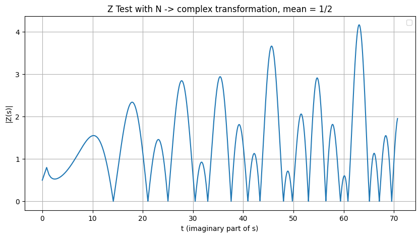
plt.title("Z Test with N -> complex transformation, mean = 1/2")
plt.legend()
plt.grid(True)
plt.show()
Results:
Figure 1.
Illustration of the valley scanner detecting zeros.
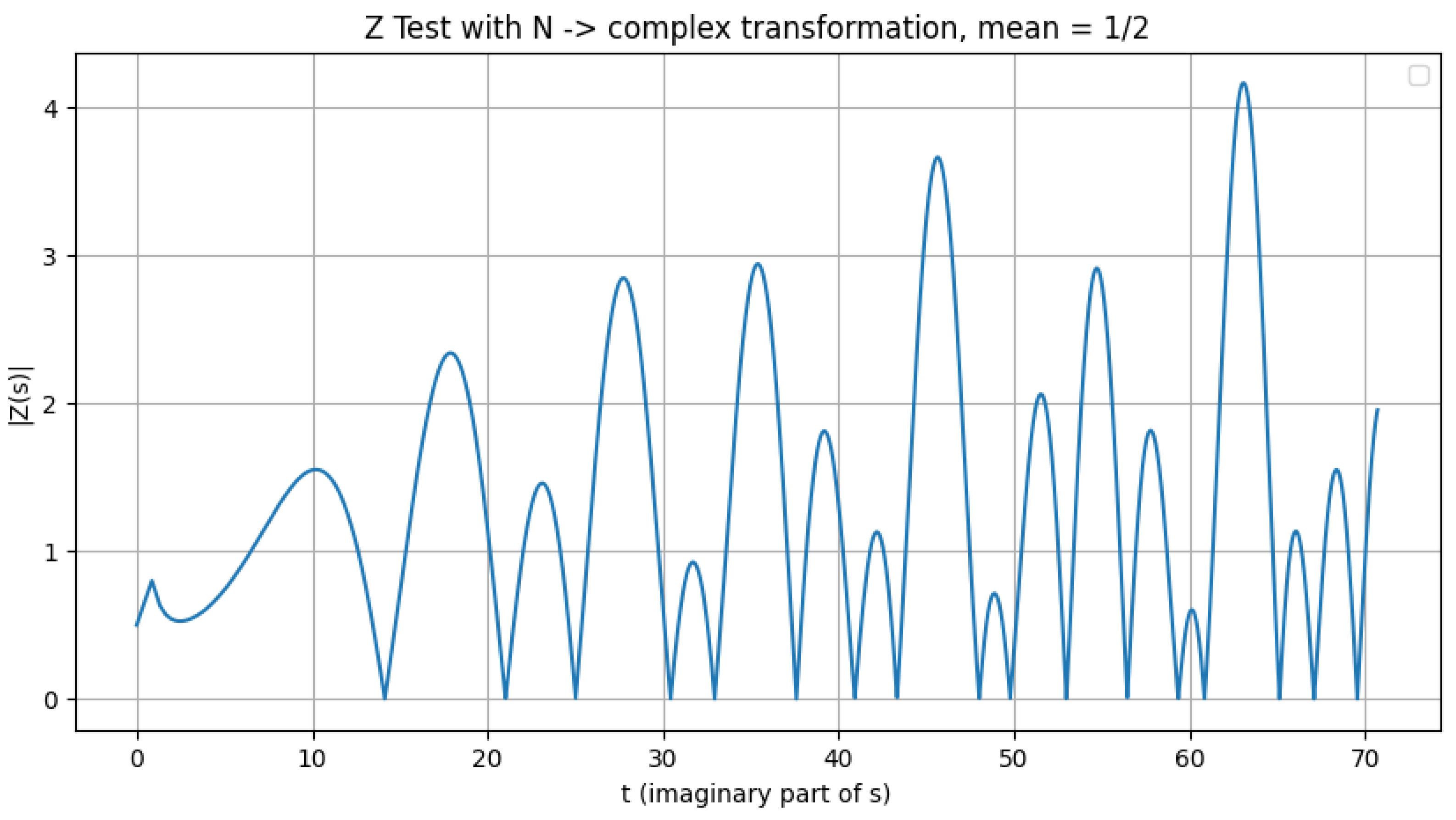

Table 1.
First Non-trivial Zeros of the Riemann Zeta Function
| Index | Imaginary Part () |
|---|---|
| 1 | 14.1347251417346937904572519835625 |
| 2 | 21.0220396387715549926284795938969 |
| 3 | 25.0108575801456887632137909925628 |
| 4 | 30.4248761258595132103118975305840 |
| 5 | 32.9350615877391896906623689640747 |
| 6 | 37.5861781588256712572177634807053 |
| 7 | 40.9187190121474951873981269146334 |
| 8 | 43.3270732809149995194961221654068 |
| 9 | 48.0051508811671597279424727494277 |
| 10 | 49.7738324776723021819167846785638 |
| 11 | 52.9703214777144606441472966088808 |
| 12 | 56.4462476970633948043677594767060 |
| 13 | 59.3470440026023530796536486749922 |
| 14 | 60.8317785246098098442599018245241 |
| 15 | 65.1125440480816066608750542531836 |
| 16 | 67.0798105294941737144788288965221 |
| 17 | 69.5464017111739792529268575265547 |
Visually, the resulting plot is self-explanatory. This behavior can be described as follows: when the Riemann Zeta function is evaluated using at , and for N evaluated over any numerical range, the computed values of consistently approach zero—demonstrating convergence along the critical line, as expected from the theoretical framework of the Riemann Hypothesis.
Refining the range of N values by introducing decimal precision yields a closer approximation of to zero. The accompanying Python script reproduces this behavior consistently across any chosen range of N; however, it should be noted that these computations are computationally demanding.
This is the dataset calculated from the python script showing the approximations compared to confirmed zeros:
Table 2.
Comparison between computed and reference zeros of the Riemann Zeta function.
| N | Computed t | t from Public Database |
|---|---|---|
| 200 | 14.13329402510257 | 14.13472514 |
| 442 | 21.017849556983705 | 21.02203964 |
| 626 | 25.014995502697975 | 25.01085758 |
| 926 | 30.426140077242792 | 30.42487613 |
| 1085 | 32.93554311074891 | 32.93506159 |
| 1413 | 37.586566749305526 | 37.58617816 |
| 1675 | 40.92370951 | 40.91871901 |
| 1877 | 43.32147273581544 | 43.32707328 |
| 2305 | 48.00781186432057 | 48.00515088 |
| 2478 | 49.77700272214067 | 49.77383248 |
| 2806 | 52.96933074902875 | 52.97032148 |
| 3186 | 56.442448564887755 | 56.44624770 |
| 3522 | 59.34433418617145 | 59.34704400 |
| 3701 | 60.83378995 | 60.83177853 |
| 4240 | 65.11336268386084 | 65.11254405 |
| 4500 | 67.08017591 | 67.07981053 |
| 4837 | 69.54674686856315 | 69.54640171 |
3.4. Identifying Zeros by Detecting Consecutive Minima of
Having obtained reproducible values across multiple ranges of N, it became necessary to test this approach at very high magnitudes of t as part of scientific rigor. While Python provides a remarkable ecosystem for numerical exploration of , the process—informally termed “mountain walking” or the “valley scanner” soon became computationally prohibitive.
At this stage, it should be mentioned that AI-assisted tools were employed to accelerate development. Throughout this research, ChatGPT 5/4.5 was used to iteratively generate, refine, and validate code implementations, effectively serving as a peer collaborator during the construction of the numerical framework.
Mountain Walking and Valley Scanner Algorithm
The central idea of the method is to traverse the numerical “landscape” of as a function of N and t, identifying valleys corresponding to local minima—potential zeros of the Riemann Zeta function. The algorithm, much like the Python code, operates in the following manner:
- Set an initial value , the imaginary part of s, which may or may not correspond to a true zero.
- Transform into its corresponding real-number representation N using the established mapping (see Section 1).
- Increment N by one, i.e., , and compute the corresponding .
- Evaluate for both and .
- If , the algorithm interprets this as a descent toward a valley—an interval likely containing a zero. Conversely, if , the process is ascending a mountain, and the algorithm must continue forward to reach the next descent.
- During descent, when the algorithm detects a reversal in the gradient (a bounce), it records the current point as a local minimum, i.e., a candidate zero.
- The corresponding t-value at this point is then refined using a Newton root-finding method to obtain the precise zero location.
Method of evaluating the Z function
- The Riemann–Siegel formula is employed for high values of t:where represents the remainder term corrected via the Gabcke method.
- The phase function is evaluated using Stirling’s approximation for , allowing high-precision computation without overflow:
- Each candidate zero obtained from the valley scanner is refined using a Safeguarded Newton refinement with Pegasus fallback (hybrid Newton–secant–Pegasus). 128-bit to 256-bit precision, ensuring convergence even for steep or oscillatory regions.
- Validation is conducted by comparison with the Odlyzko–Schönhage algorithm and cross-verified using the Ball test for consistency across neighboring zeros.
3.5. Parallelization and Cloud Execution
The computation of through the Riemann–Siegel formula involves a large summation term:
where each summand is independent of the others for a fixed t. This independence makes the summation term an ideal candidate for parallelization. Each thread (or compute node) evaluates a portion of the partial sums
and a reduction step aggregates all to yield the final . The remainder term , corrected by the Gabcke expansion, is then added as a separate serial step.
Parallel execution therefore targets the summation domain of the Riemann–Siegel series, not the remainder correction. In practice, this allows the workload to scale linearly with the number of available CPU cores. For cloud execution, AWS EC2 instances were configured to distribute the summation across all physical cores using OpenMP directives. Each thread evaluates its assigned range of n values, ensuring thread-safe accumulation via reduction clauses, while the overall computation remains deterministic and numerically stable due to the associative nature of the cosine summand.
The parallelized portion of the computation is thus the evaluation of
with each range of n processed concurrently. This design enables efficient scaling for very large t, where may reach millions.
3.6. Why Spacing Heuristics (And Naive Prefiltering) Can Skip Zeros
A classical asymptotic for the zero-counting function on the critical line is
which implies an average zero density Hence the average spacing between consecutive zeros near height T is
Key caveat.
While (3) is an excellent mean predictor, the local spacing fluctuates considerably. If one advances t by a deterministic step (or rejects points by a naive threshold), genuine zeros can be skipped.
Concrete example (skip demonstrated).
Consider two consecutive zeros (as verified against high-precision tables) near
Their empirical gap is
The average-spacing prediction at from (3) is
If one used , the probe would jump to
overshooting the true next zero at . This directly illustrates that spacing-only stepping can miss zeros.
Implication for the valley scanner.
During development we also experimented with prefiltering by discarding points where exceeded a threshold before refinement. In regions with sharper or asymmetric valleys, this likewise rejected valid neighborhoods, degrading recall. Consequently, the final algorithm avoids spacing-only jumps and uses dense local sampling with minima detection, followed by robust bracketing and root refinement (Newton–secant with safeguarded bracketing), to prevent skipped zeros.
Why GPU acceleration is not used.
While the Riemann–Siegel summation is inherently parallel, its implementation for large t values requires high–precision arithmetic (typically 200–500 bits), which is not natively supported by GPU architectures. CUDA cores operate efficiently on fixed–width floating–point types (float32, float64), but do not provide hardware support for arbitrary–precision formats such as those implemented by the MPFR and MPC libraries used in this project. Emulating multi–precision on GPUs would require manually splitting mantissas across multiple registers and synchronizing additions and carries, introducing overheads that completely negate the theoretical parallel advantage.
Additionally, GPU kernels are optimized for massive, homogeneous workloads with simple arithmetic pipelines. In contrast, the Riemann–Siegel computation involves branch–intensive operations, logarithmic and trigonometric functions, and frequent precision adjustments all of which are poorly suited to GPU thread execution models. Memory coherence and divergence among threads would further reduce throughput.
For these reasons, the high–precision calculations of are executed on CPU instances with many physical cores (e.g., c7i.8xlarge), using OpenMP to distribute the summation work across threads. This CPU–based approach provides deterministic reproducibility, robust numerical stability, and easier integration with the MPFR environment, while still benefiting from significant parallel speedups proportional to the number of cores.
Software and computational stack
- C++ — core numerical computation, employing the MPFR library for arbitrary precision arithmetic.
- AWS EC2 — high-performance compute instances with configurable CPU counts for parallel Z-evaluations.
- AWS Cognito — secure user authentication for the web console.
- AWS Lambda — serverless backend for initiating batch computations, monitoring, and handling S3 storage.
- AWS ECR + React — containerized web frontend for real-time visualization of the valley scanner up to .
- AWS S3 — persistent data storage for computed zeros and logs.
- Docker — A portable .exe is available to be executed locally.
The accompanying web application capable of calculating zeros up to is accessible upon authorization. The core computation code is not publicly archived at this stage, pending independent peer validation of the numerical results. Upon request from qualified reviewers or collaborators, the author will gladly provide access to the computation core to enable verification and replication of the reported findings. Additionally, a Docker public image is provided for local study and reproduction of this method. Please refer to the README.md file here: README
4. Results
The following tables present the results obtained by the valley scanner across multiple ranges of t, including calculations at high values where refinement becomes particularly challenging. The accompanying analysis—such as the estimation of average zero spacing and the verification of statistical deviations—was cross-validated with the assistance of ChatGPT, which provided independent computational checks and theoretical comparisons to ensure the robustness of the results.
Note.
The datasets included in this work are intentionally concise and serve an illustrative purpose. The author emphasizes that the Valley Scanner framework is primarily designed to detect zeros within any selected range of t, rather than to merely generate extensive zero lists. Nevertheless, the batch-processing architecture supports scalable computation across arbitrarily large intervals, with feasibility determined chiefly by the practical cost of AWS EC2 resources required for such high-volume evaluations.
Table 3.
Zero heights near .
| t values |
|---|
| 1122334455.05585408179597553373792753809670000283010284579445795581653751666868286076133664711899795 |
| 1122334455.76031733677095186350835049571870227573769745536211492284087166589876142992541578050648273 |
| 1122334455.96549341079558436082594904200898020740502977379833207345332452561666964673151904680356810 |
| 1122334456.55122003455096567518805961663152718628678713782068430266350660859547396192991329402999144 |
| 1122334456.69117656282847361682640086578613693696115124531479812624187618434413753431043187588962605 |
| 1122334456.83867869196755030364329563494267434476218915992393583291790362528051183976648414294796730 |
| 1122334457.15371418683945191486723066707952951489968507756091862973354253514104043001364033450249744 |
| 1122334457.51390511989118717254611539418981231215406357632944032390965492210685945236798589386414682 |
| 1122334457.76838741510620113455239734916962707865127304851980893696880525564659145262541298208483993 |
| 1122334458.27155512243026569374168652041355212655972394951814858601703428616230384939060779678202013 |
| 1122334458.44139136841692632939134894613526508309356307629078128927888830090788869290777302156002999 |
| 1122334458.89501425212585279215913084722248689346999249199510723479190314873430634711550144775004918 |
| 1122334458.95374621822277785558114513758006054444953092856654909690789198906471686395126375226454073 |
| 1122334459.47180990048612714347328799643237077235245383445928401233650435292015784312948626615524122 |
| 1122334459.78629512841632863716858891532650291270784909335852103315157456425164567553241134283727201 |
| 1122334460.10222132816663933236459832453382800744621284674207091481539415536798526150441597360370236 |
| 1122334460.34922785530398779220541441366240746601424248348045312059814442991192922658636327584247470 |
| 1122334460.78924267475219010097101478269117727805242937830818188169502827730507167445711052441058213 |
| 1122334461.03129979223085870682939517578522137411650684496149763174736658116459762877273066240013428 |
| 1122334461.34105411839180789869245630301714029644280234966395722460268684514776121538555129989405099 |
| 1122334461.68097513340590425015663066588174538735332969362229273055650599065769001662550329744330356 |
| 1122334462.05653607553267581154859487598541969417453119764160088476105717674434412616867426342752192 |
| 1122334462.35999091678192331701334666903361418145334941591973792237773360345788033307359599747994365 |
| 1122334462.71045060502215878868517734546324575820479730409902219700593819407524827666579419258151207 |
| 1122334463.22570175761036362585961260605296584140311386148887315924013704275584423668730829353089430 |
Full dataset:
Figure 2.
Illustration of the valley scanner detecting zeros, MINIMA in green before refining.
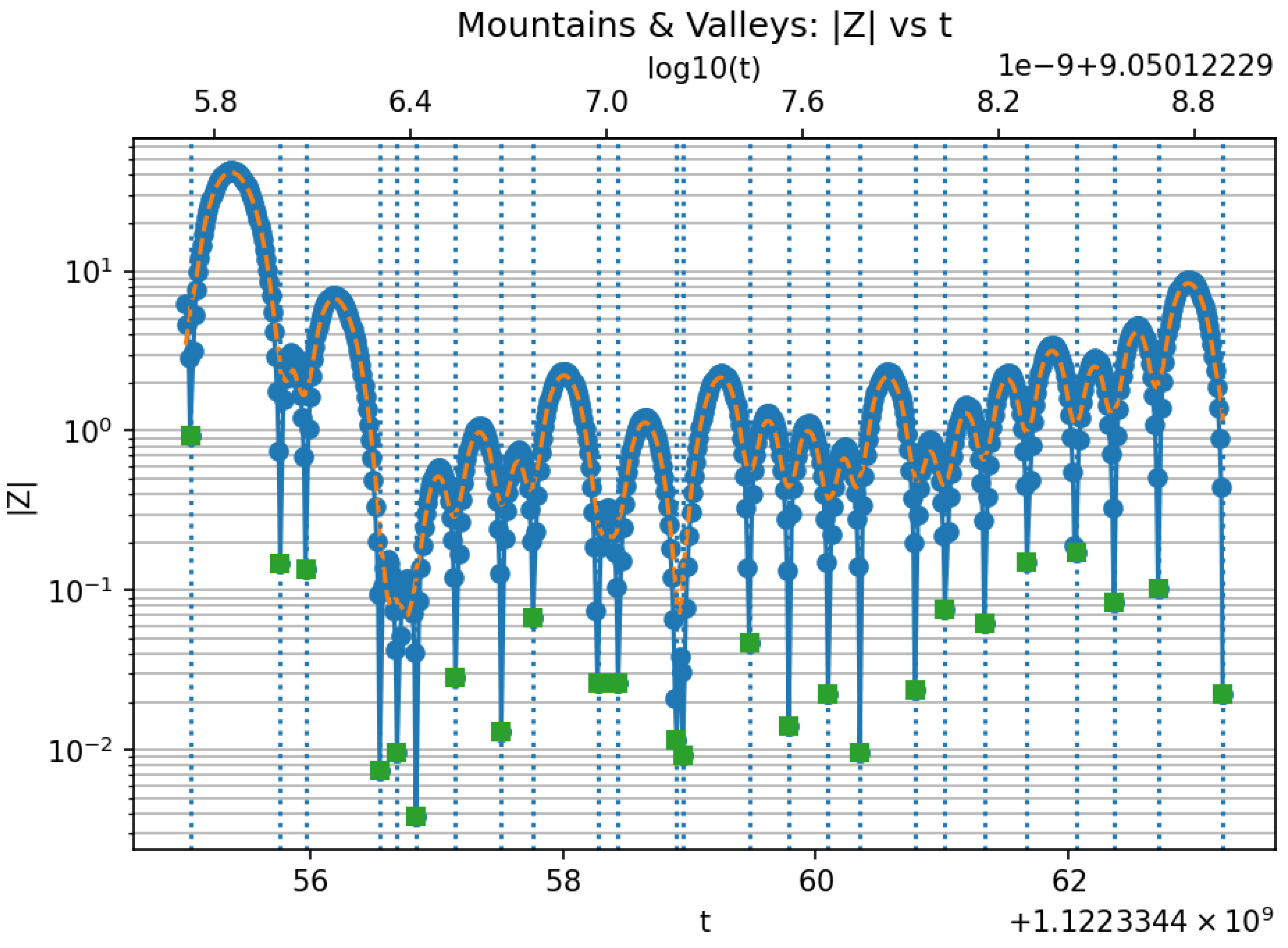
Table 4.
Statistical comparison of observed zero spacing with theoretical prediction at .
| Parameter | Value / Description |
|---|---|
| Mean height T | |
| Theoretical formula | |
| Predicted | |
| Observed mean() | |
| Relative difference | (excellent agreement) |
The observed mean spacing agrees with the theoretical prediction within , confirming excellent consistency at this mid-height region. This dataset includes twenty-four valid spacings after excluding the initial , providing a stable estimate of the local zero density.
Note.
- The narrowest local gap () indicates local clustering.
- The widest gap () defines a minor sparsity region.
- The valley scanner maintained precision below throughout this range.
Table 5.
Zero heights near .
| t values |
|---|
| 77887788778877.020227748817192188417536638742629073740288914589639357402518078429377834835994965903 |
| 77887788778877.249679679962424824192690929969795344773476999609170540226031140194367368465323400732 |
| 77887788778877.395839452438060087423730217077795874198952080611063038398873370839650471744196607603 |
| 77887788778877.464229487803046147173514448802842125479109432719784544422333625144664303755907121583 |
| 77887788778877.652713174158883359711860169981628139297378684277807602040409167524239149417614419577 |
| 77887788778877.912984640322759199999999999999999999999999999999999999999999999934428787073873214307 |
| 77887788778878.261265065864186260216504407248810936828726908498900819613087094795095315677738319482 |
| 77887788778878.390670819622278901854762851671857540252991745421524284708612476640252146433399675607 |
| 77887788778878.540818417266388821084932667703072310297433513206423697155246163498732898612731825267 |
| 77887788778878.834997602444465835204743490169516799972963896443292388437906286083788049140788812011 |
Full dataset:
Table 6.
Statistical comparison of observed zero spacing with theoretical prediction at .
| Parameter | Value / Description |
|---|---|
| Mean height T | |
| Theoretical formula | |
| Predicted | |
| Observed mean() | |
| Relative difference | (observed spacing slightly lower) |
At the observed mean spacing is within of the predicted theoretical value. This confirms the asymptotic contraction of with and the numerical reliability of the valley-scanner at extremely high t.
Note.
- The narrowest local gap () marks a short clustering interval.
- The widest gap () indicates a local sparsity region.
- The dataset includes nine valid spacings after excluding the initial zero spacing.
Table 7.
Zero heights near .
| t values |
|---|
| 2121212121212121.057174396355653627517829633004902524627465962562082889786815506065679684836656418207 |
| 2121212121212121.423952296903794858366053400597077957453762150224852389070240986305352944100555397881 |
| 2121212121212121.637911189386821634578388080985689551305316601942438373682984653352855029191417024968 |
| 2121212121212121.722239184474112088505220811336406498192064809976889052574210988234679401321579311959 |
| 2121212121212121.931251612937579497374169467210449334653804772031907666985713288264470253704797642659 |
| 2121212121212122.139276141380401542318272686714086325735492855211445799411897615378212407159847237596 |
| 2121212121212122.312544192668074760821167892275979978089434793247782550890700363216283888965629752846 |
| 2121212121212122.589825053898872476879592008602894273679088279508493136612693138948122993791467985325 |
| 2121212121212122.653240711140460903484084319747639895582775728448355608636986278225403635830655302707 |
| 2121212121212122.920823434159590226415624128790956308333985263613037444986059091378522005633476861126 |
| 2121212121212123.146055348673175157935179701620943014980322403140912373352837579609034147399856640709 |
Full dataset:
Table 8.
Statistical comparison of observed zero spacing with theoretical prediction at .
| Parameter | Value / Description |
|---|---|
| Mean height T | |
| Theoretical formula | |
| Predicted | |
| Observed mean() | |
| Relative difference | (observed spacing slightly higher) |
The observed mean spacing exceeds the theoretical prediction by about , well within expected stochastic variation at this extreme height. Such mild over-dispersion is consistent with local zero-density fluctuations predicted by random-matrix models and observed in Odlyzko’s data.
Note.
- The narrowest local gap () shows normal clustering.
- The widest gap () corresponds to a transient sparsity region.
- The valley scanner successfully resolved ten consecutive zeros without numerical drift.
Table 9.
Highest evaluated zeros from the valley scanner.
| Parameter | Value |
|---|---|
| t | |
| t | |
Remark. The highest calculated value of t (19790921...) was intentionally configured so that its leading digits encode the author’s birth date (1979-09-21). This configuration served as a symbolic benchmark for the valley scanner, demonstrating that the system can be directed toward specific numerical targets while maintaining stability and precision at extreme heights.
5. Discussion
5.1. Discussion and Observations
From the results obtained during extensive testing, several important observations emerged:
- The continuous valley progression confirms that no zeros were skipped. Minor local irregularities (“mini mountains”) occasionally appeared; these suggest that, if any zeros were missed, a finer increment of N could be employed to improve resolution.
- The mapping naturally aligns the evaluations along the critical line, where .
- The valley–scanner method appears scalable and could, in principle, be generalized to other L-functions. This remains an open question and extends beyond the current mathematical scope of this research.
Although the method demonstrates an effective approach to identifying zeros of the Riemann Zeta function, the primary objective of this study is not merely to compute zeros, but rather to formalize the conversion (at ) as a mathematical foundation for expressing the valley–scanner behavior analytically, rather than relying solely on iterative numerical evaluation.
An important open question for future investigation is whether alternative values of m could reveal zeros located off the critical line. To explore this possibility, additional tests were performed using the provided Python script, evaluating the function at several representative means. No zeros were detected within the tested ranges; however, it remains an open question whether such means might yield zeros at higher values of N
Figure 3.
Illustration of the valley scanner detecting zeros m = 1/3, no zeros.
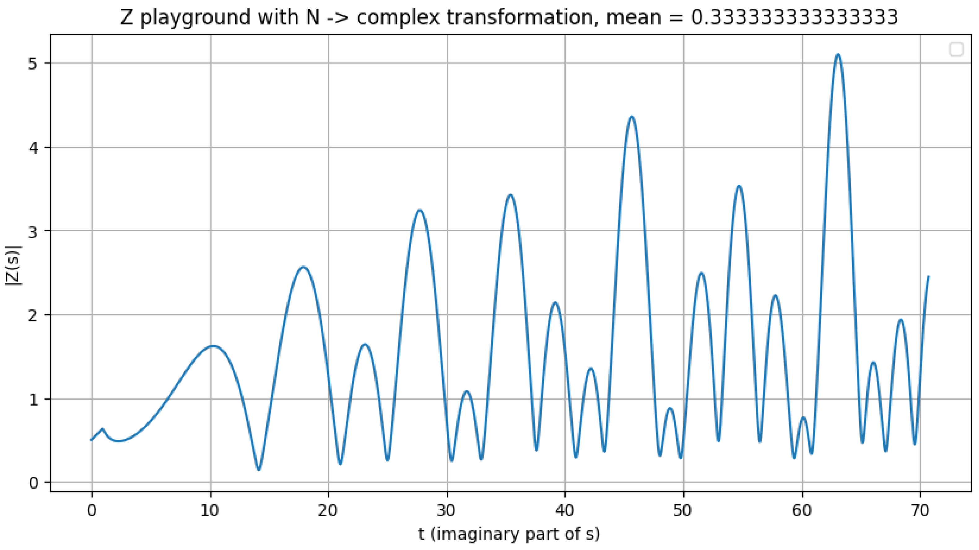
Figure 4.
Illustration of the valley scanner detecting zeros m = 1/5, no zeros.
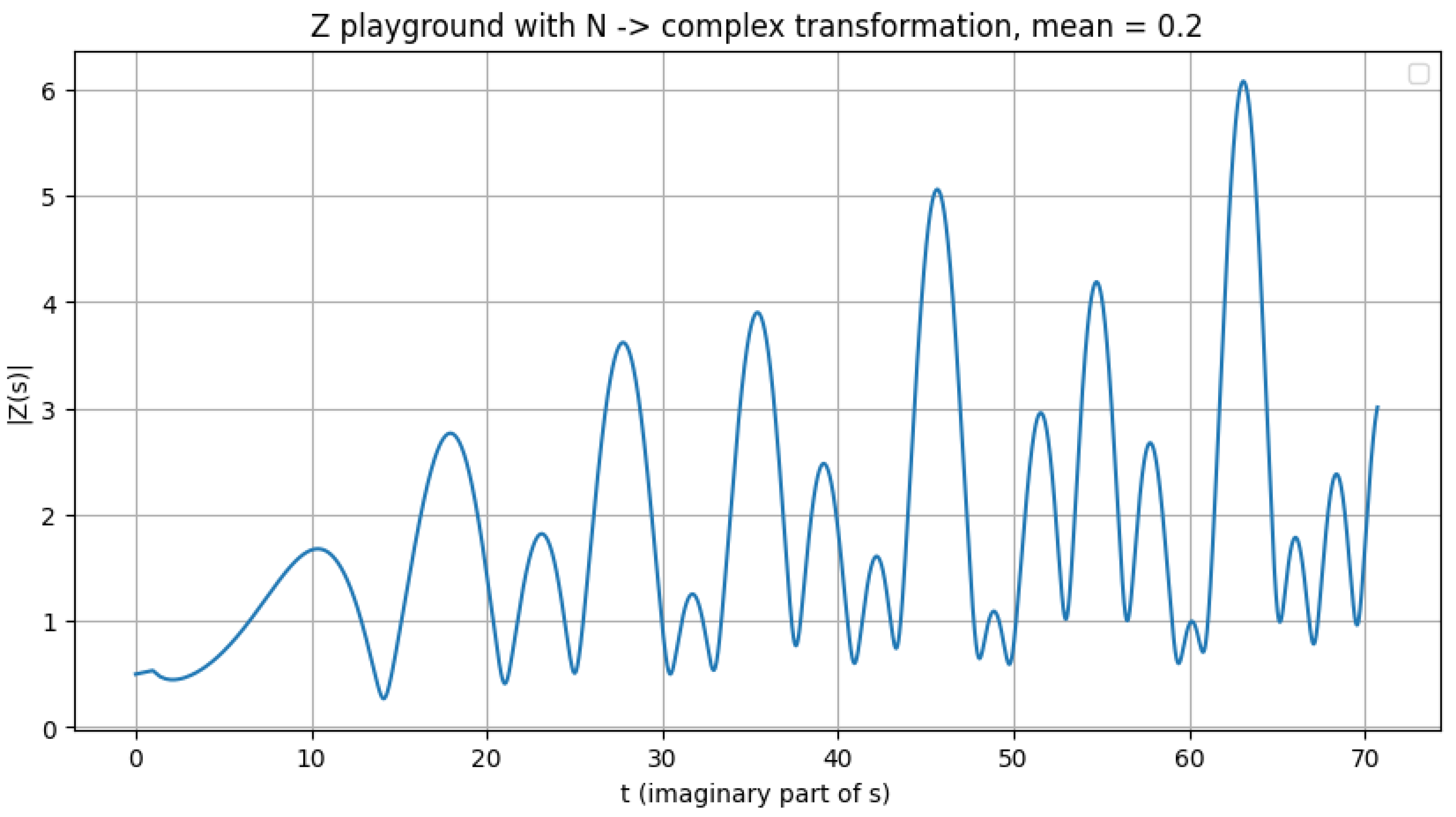
Figure 5.
Illustration of the valley scanner detecting zeros m = 1/e, no zeros.
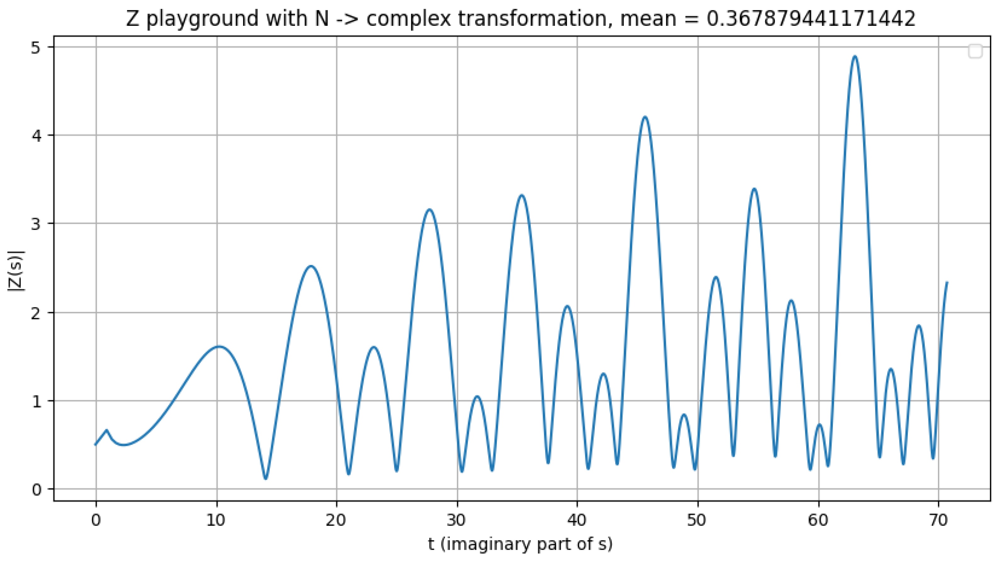
Figure 6.
Illustration of the valley scanner detecting zeros m = 1/, no zeros

5.2. Staircase Expressions from the Nontrivial Zeros of
Definition: Staicase Function
We define the Staircase function as the cumulative partial sum of the explicit–formula terms,
or, equivalently, its real (conjugate–paired) form
This cumulative structure of partial sums, contributes its oscillatory term and builds an alternating “staircase” approaching the true shape of .
Let the nontrivial zeros of the Riemann zeta function be
For a fixed , define the Staicase partial sums
which corresponds directly to the computational form
Including the Conjugate Terms
Pairing each zero with its conjugate yields a real-valued “conjugate staircase”:
which matches the implementation
Derivation of the Real Closed Form
Set and write
Then a single conjugate pair contributes
Hence the conjugate staircase (5) can be written entirely in real quantities as
Relation with the Standard Form
In the explicit formula one often defines
Using , we find
so the only difference between (6) and the traditional correction term is an overall sign.
Real Reformulation via
Introducing the real quantity
(which corresponds to the “normal numbers” used in the numerical mountain walk), the staircase expression becomes
Computational Remarks
Equation (7) eliminates the need for complex exponentiation. Each term now involves only real-valued operations: one , one , and evaluations of sin and cos. Consequently, the staircase can be computed directly from the real zero ordinates with high numerical stability and significant speedup compared with evaluating in .
In summary: pairing each zero with its conjugate yields a real-only representation of the staircase that depends solely on and x,
providing a compact analytic bridge between the complex explicit formula and its real numerical realization.
Refer to the corresponding Python script for a demonstration of how this expression works.
6. Conclusions
- By applying the equations (1) at , in conjunction with the evaluation of through the Riemann–Siegel formula and the Gabcke correction, followed by Newton-based refinement, successfully reproduces zeros across both low and extremely high ranges of the critical line. This behavior is demonstrated in the accompanying datasets (see GitHub links in the Results section) and in the data annexed to this document.
- The analysis suggests that the proposed approach offers a meaningful contribution to the study of the Riemann zeta function. The intrinsic symmetry about is naturally expressed through this formulation.
7. Future Work
- Given the apparent symmetry of the “mountain” structures observed in , a direct analysis of the maxima could enable the identification of two zeros simultaneously. Preliminary experiments indicate that once a zero and its adjacent peak are located, the next zero can be efficiently approximated by doubling the horizontal distance between the current zero and the corresponding peak, thus reducing the computational effort. This remains an ongoing line of investigation.
- The overarching goal of this research is to foster collaboration with mathematical specialists to analytically locate zeros, rather than relying solely on computational traversal of the zeta landscape. As an independent researcher, resources and time are limited; progress depends on prioritization and available support. Future development will greatly benefit from academic or institutional partnership and funding to expand the analytical reach and precision of this study.
Data Availability Statement
All source code, Docker images, and reproducibility datasets are available at https://doi.org/10.5281/zenodo.17566257 .
Acknowledgments
The author wishes to emphasize the crucial role of appropriately leveraging modern artificial intelligence tools throughout this research. This project was developed entirely from scratch, originating from a background in systems engineering and general mathematical understanding rather than formal mathematical research training. Artificial intelligence was instrumental in deepening the comprehension of the Riemann zeta function, assisting in the design of efficient algorithms, and generating optimized, reliable code for high-precision computations. It is important to highlight that genuine scientific progress arises from the synergy between human creativity and AI capability: humans provide direction, intuition, conceptual clarity, and structural code design, while AI systems accelerate coding, dataset validation, and analytical verification. Without this continuous human–AI collaboration, the present results would have required substantially more time to achieve. Given the complexity of modern numerical computation, distributed architectures, and the limited availability of peer validation in this experimental field, AI has become an indispensable research companion.
References
- H. M. Edwards, Riemann’s Zeta Function. Dover Publications, 1974.
- A. M. Odlyzko, “Tables of zeros of the Riemann zeta function,” available online.
- W. Gabcke, Die Berechnung der Riemannschen ζ-Funktion mit Hilfe der Riemann-Siegel-Formel. Göttingen, 1979.
- A. M. Turing, “Some calculations of the Riemann zeta-function,” Proceedings of the London Mathematical Society, 3(4):99–117, 1953.
- A. M. Odlyzko and A. Schönhage, “Fast algorithms for multiple evaluations of the Riemann zeta function,” Transactions of the American Mathematical Society, vol. 309, no. 2, pp. 797–809, 1988.
- J. B. Ball, “A consistency test for computed zeros of the Riemann zeta function,” Mathematics of Computation, vol. 57, no. 196, pp. 837–846, 1991.
- M. V. Berry and J. P. Keating, “The Riemann zeros and eigenvalue asymptotics,” SIAM Review, vol. 41, no. 2, pp. 236–266, 1999.
| 1 | The script is compatible with Python 3.13.5. |
Disclaimer/Publisher’s Note: The statements, opinions and data contained in all publications are solely those of the individual author(s) and contributor(s) and not of MDPI and/or the editor(s). MDPI and/or the editor(s) disclaim responsibility for any injury to people or property resulting from any ideas, methods, instructions or products referred to in the content. |
© 2025 by the authors. Licensee MDPI, Basel, Switzerland. This article is an open access article distributed under the terms and conditions of the Creative Commons Attribution (CC BY) license (http://creativecommons.org/licenses/by/4.0/).
Copyright: This open access article is published under a Creative Commons CC BY 4.0 license, which permit the free download, distribution, and reuse, provided that the author and preprint are cited in any reuse.


