
Submitted:
13 November 2025
Posted:
17 November 2025
You are already at the latest version
Abstract
High-resolution Digital Terrain Models (DTMs) are essential for precise terrain analy-sis, yet their production remains constrained by the high cost and limited coverage of LiDAR surveys. This study introduces a deep learning framework based on a modified Residual Channel Attention Network (RCAN) to super-resolve 10 m DTMs to 1 m res-olution. The model was trained and validated on a 568 km² LiDAR-derived dataset us-ing custom elevation-aware loss functions that integrate elevation accuracy (L1), slope gradients, and multi-scale structural components to preserve terrain realism and ver-tical precision. Performance was evaluated across 257 independent test tiles repre-senting flat, hilly, and mountainous terrains. A balanced loss configuration (α = 0.5, γ = 0.5) achieved the best results, yielding Mean Absolute Error (MAE) as low as 0.83 m and Root Mean Square Error (RMSE) of 1.14–1.15 m, with near-zero bias (–0.04 m). Er-rors increased moderately in mountainous areas (MAE = 1.29–1.41 m, RMSE = 1.84 m), confirming the greater difficulty of rugged terrain. Overall, the approach demonstrates strong potential for operational applications in geomorphology, hydrology, and land-scape monitoring, offering an effective solution for high-resolution DTM generation where LiDAR data are unavailable.
Keywords:
DTMs
; neural networks
; RCAN
; super resolution
; accuracy assessment
1. Introduction
Digital Terrain Models (DTMs) are fundamental tools for analyzing and modeling Earth surface processes, supporting applications in hydrology, geomorphology, natural hazard assessment, and environmental planning [11,26,35]. They provide raster-based, geo-referenced representations of the Earth's surface elevation, capturing topographic variability essential for surface water modeling, landscape evolution, and risk analysis. High-resolution DTMs, typically derived from airborne LiDAR or UAV photogrammetry, offer detailed depictions of terrain morphology but are limited by high acquisition costs, complex logistics, and restricted spatial coverage, particularly in remote or densely vegetated areas [1,5,12].
In contrast, global DTMs such as the Shuttle Radar Topography Mission (SRTM), ALOS World 3D, and Copernicus GLO-30 provide near-global coverage at spatial resolutions of 30 meters or more, enabling regional to global-scale studies [19,24]. However, these coarser models often fail to represent fine-scale topographic details, especially in mountainous or urban environments, reducing their suitability for high-precision modeling tasks. This trade-off between spatial resolution and coverage has motivated the development of super-resolution (SR) methods that aim to computationally enhance the resolution of coarse DTMs, providing a cost-effective alternative for terrain refinement [2,38,44,49].
Super-resolution techniques, originally developed in the image-processing field, reconstruct high-resolution images from one or more low-resolution inputs [36]. When applied to elevation data, the challenge lies in recovering fine-scale geomorphological structures from sparse inputs. Traditional SR approaches can be broadly classified into interpolation-based, reconstruction-based, and learning-based methods [41,46]. Interpolation approaches such as bilinear, bicubic, Kriging, or Inverse Distance Weighted (IDW) are simple and computationally efficient but tend to over smooth terrain features, failing to preserve ridges, cliffs, or slopes [16,21,39]. Reconstruction-based methods use gradient or edge constraints to improve surface detail, yet their effectiveness declines under high upscaling factors or in heterogeneous terrain [15,34].
Learning-based methods, especially deep learning (DL) approaches, have recently shown great promise by learning non-linear relationships between low-resolution and high-resolution elevation data. Early frameworks relied on manifold learning [6], sparse coding [40], or patch-based dictionary matching [38], but these were computationally expensive. The introduction of convolutional neural networks (CNNs) enabled end-to-end training from paired datasets, and models such as Super-Resolution Convolutional Neural Network (SRCNN), Enhanced Deep Residual Networks (EDSR), Super-Resolution Generative Adversarial Network (SRGAN), Enhanced SRGAN (ESRGAN), and Residual Channel Attention Network (RCAN), originally designed for natural image enhancement, have been successfully adapted for DTM super-resolution [8,18,20,37,45,47]. Among these, the Residual Channel Attention Network (RCAN) is particularly effective due to its ability to recover high-frequency terrain details using residual blocks and channel-wise attention [43].
Despite these advances, applying image-based models directly to elevation data presents unique challenges. DTMs represent continuous surfaces with geometric properties such as slope, aspect, and curvature, which are not typically considered in models trained on natural images. As a result, standard CNN-based methods may produce elevation inconsistencies, loss of geomorphological structure, or artifacts affecting drainage networks and valley boundaries [13,27]. Furthermore, deep learning models often generalize poorly across different terrain types and rarely incorporate topographic constraints or uncertainty quantification [9,29].
To address these limitations, recent studies have integrated terrain-specific descriptors such as slope, curvature, and roughness into model architectures or loss functions [22,45]. These terrain-aware strategies reinforce physical consistency and improve the realism of reconstructed surfaces. Multi-component loss functions combining pixel-wise accuracy (L1, L2), perceptual similarity (SSIM), and gradient-based terrain consistency have further enhanced both numerical precision and structural coherence [37,48]. Hybrid frameworks, such as detrending-based deep learning (DTDL), have also been proposed to separate large-scale elevation trends from high-frequency residuals, allowing more effective learning of fine-scale patterns [28].
Beyond deep learning, probabilistic and geostatistical approaches have treated DTM super-resolution as a non-unique reconstruction problem, modeling multiple plausible fine-resolution surfaces consistent with the same coarse data [2,4]. Methods based on variograms [10,17] or Multiple-Point Statistics (MPS) using training images [23,30,33] can reproduce spatial structures realistically but are computationally demanding and rely on suitable training data [32,42].
Despite substantial methodological progress, generating accurate high-resolution DTMs remains a challenge, especially in topographically complex regions such as high mountain Asia [14], where global DTMs like SRTM or ASTER GDEM fail to capture sharp terrain discontinuities. Preserving key landform features such as ridgelines, drainage channels, and valley floors is critical for hydrological and environmental modeling [3,25]. Moreover, performance must be assessed not only through error metrics such as RMSE or MAE but also in terms of geomorphological realism and through the consistency of derived terrain parameters [7,31].
The present study proposes a deep learning-based super-resolution framework for DTM enhancement using the RCAN model, optimized through terrain-aware loss functions that incorporate domain-specific elevation and slope information. The research aims to (1) identify and evaluate the most effective loss function for terrain super-resolution and (2) fine-tune the corresponding weights to balance elevation accuracy and structural preservation. Using a 568 km² LiDAR-derived dataset covering diverse terrain types, the model is trained to generate 1 m resolution DTMs from 10 m inputs. Model performance is evaluated through statistical and structural metrics across flat, hilly, and mountainous areas. The results demonstrate that combining deep learning with geomorphological informed loss functions provides a practical and scalable approach for producing high-resolution DTMs from widely available coarse datasets.
2. Materials and Methods
2.1. Overview of the Workflow
The proposed workflow is structured into two main phases. In the first phase, several custom loss functions were developed and assessed to determine which configuration best improves DTM reconstruction quality. In the second phase, the selected loss function was fine-tuned by adjusting the relative balance between its components to further optimize model performance. The backbone of the super-resolution framework is the Residual Channel Attention Network (RCAN), an advanced neural architecture designed to upscale spatial data while preserving fine-scale structural details. For this study, RCAN was specifically adapted for terrain data by incorporating loss components sensitive to elevation-dependent features such as slope gradients.
2.2. Dataset Description
The dataset consists of 568 high-resolution DTM tiles freely provided by the Italian Ministry of the Environment and Energy Security (MASE) (https://sim.mase.gov.it/portalediaccesso/mappe/#/viewer/new) (Figure 1). Each tile covers a 1 km × 1 km area and was derived from airborne LiDAR data. The dataset includes diverse morphological contexts, flat plains, hilly regions, and mountainous areas, ensuring that the model is trained on a wide range of topographic conditions.
For model preparation, each high-resolution tile (1 m, 1000 × 1000 pixels) was down sampled using an average aggregation technique to generate a corresponding low-resolution version at 10 m resolution (100 × 100 pixels). The dataset was then divided into three subsets: training, validation, and testing tiles. These paired datasets served as inputs (low-resolution) and targets (high-resolution) for model training and evaluation.
2.3. RCAN Model Architecture
To reconstruct high-resolution DTMs from coarse inputs, a modified version of the Residual Channel Attention Network (RCAN) was implemented. RCAN is particularly effective for elevation data, as it captures both local structural features and absolute elevation information.
The adapted architecture (Figure 2) begins with a shallow feature extraction layer consisting of a single 2D convolution followed by a ReLU activation, which maps the single-channel elevation input to a higher-dimensional feature space. The core of the network comprises ten Residual Channel Attention Blocks (RCABs), selected to achieve a balance between computational efficiency and performance.
Each RCAB contains two convolutional layers interleaved with ReLU activations to extract local spatial features. A Squeeze-and-Excitation (SE) block adaptively recalibrates channel-wise feature responses through global average pooling, two fully connected layers, and a sigmoid activation function that scales the feature maps. This channel-attention mechanism enhances the model’s ability to focus on informative terrain patterns while maintaining the integrity of elevation information. The residual structure within each block allows for efficient gradient propagation and minimizes information loss during training.
Following the deep feature extraction, a progressive up-sampling module increases spatial resolution through three stages. The first stage up samples by a factor of 2.5 using bilinear interpolation, while the subsequent two stages perform 2× up sampling each. A convolutional layer and a Leaky ReLU activation to refine intermediate representations follow each up-sampling step. The final output layer maps multi-channel features back into a single elevation channel, yielding the predicted high-resolution DTM.
2.4. Custom Loss Functions
To account for terrain-specific properties during model optimization, four custom loss functions (LF1–LF4) were developed and evaluated:
- LF1: Combined L1, L2, and slope-based errors.
- LF2: Weighted L1 loss emphasizing elevation deviations.
- LF3: Laplacian pyramid loss preserving multiscale edge details.
- LF4: Elevation gradient loss combining L1 error with slope consistency.
Each loss function was used independently to train the RCAN model for 100 epochs on identical training and validation datasets. The best-performing model from each configuration was selected based on validation RMSE and SSIM metrics.
The loss formulations are expressed as follows:
where:
total loss = α * l1 + β * l2 + γ * slope
total loss = α * l1 + β * elevation_aware_loss
total loss = α x l1 + β x lap + γ x grad loss
total loss = α × L1 + γ × Slope
- α, β, γ represent weighting coefficients balancing the contribution of each component;
- L1 loss penalizes absolute elevation differences between predicted and reference DTMs;
- L2 loss penalizes squared differences, emphasizing large errors;
- Slope loss enforces gradient consistency in both x and y directions;
- Elevation-aware loss applies spatial weighting based on absolute elevation values;
- Laplacian pyramid loss preserves edge sharpness and fine-scale details.
Among these, LF4, combining L1 and slope-based gradient terms, achieved the best overall performance. To fine-tune this configuration, three weight combinations were tested: (α = 0.8, γ = 0.2), (α = 0.5, γ = 0.5), and (α = 0.2, γ = 0.8). Each configuration was trained for 100 epochs, and the best-performing checkpoint was selected for final testing.
2.5. Training Setup and Implementation
All experiments were conducted using the PyTorch framework on Google Colab (V3) equipped with a Tesla T4 GPU. The learning rate was fixed at 5 × 10⁻⁶, the batch size was set to 4, and random seeds were initialized for reproducibility. Model checkpoints were saved periodically, and the final model was selected based on the lowest validation RMSE across epochs.
2.6. Evaluation Metrics
Model performance was assessed on a per-tile basis using standard statistical and perceptual metrics, including Root Mean Square Error (RMSE), Mean Absolute Error (MAE), Peak Signal-to-Noise Ratio (PSNR), and Structural Similarity Index (SSIM). Visual assessments were also performed through signed error maps and residual histograms to identify spatial patterns of error, particularly in areas with steep slopes or complex morphology.
2.7. Use of Generative AI
Generative Artificial Intelligence (GenAI) tools, specifically ChatGPT (OpenAI, San Francisco, CA, USA), were used to assist in the language refinement and formatting of this manuscript. The AI was not used for generating data, designing experiments, analyzing results, or interpreting findings. All scientific content, methods, and conclusions were entirely developed and validated by the authors.
3. Results
3.1. Quantitative Evaluation of Loss Functions
To assess the effectiveness of the proposed terrain-aware loss formulations, four distinct loss functions (LF1–LF4) were implemented and tested within the RCAN-based DTM super-resolution framework. Each configuration was trained independently for 100 epochs under identical conditions, including model architecture, dataset, and training parameters, to ensure a consistent basis for comparison. The optimal checkpoint for each configuration was selected according to the minimum validation loss.
Model performance was quantitatively evaluated using the Root Mean Squared Error (RMSE), Mean Absolute Error (MAE), Peak Signal-to-Noise Ratio (PSNR), and Structural Similarity Index (SSIM). The averaged results across all test tiles are summarized in Table 1.
Among the tested configurations, LF4, which combines the L1 elevation error with a slope-consistency term, achieved the best overall performance. It recorded the lowest test RMSE (1.647 ± 0.490) and MAE (1.217 ± 0.382), while maintaining a high SSIM (0.992 ± 0.004) and the highest PSNR (49.304 ± 3.493 dB). These results indicate superior generalization capability and enhanced preservation of both elevation fidelity and terrain structure (Figure 3).
In contrast, LF2, which employs an elevation-weighted L1 term based on deviation from the mean, produced the weakest performance, with a test RMSE of 36.843 ± 13.991 and an MAE of 24.140 ± 9.442. The substantial degradation suggests that the adaptive weighting mechanism introduced instability during training, possibly resulting in overfitting in smoother regions and elevated error in high-relief terrain (Figure 4).
LF1, a composite loss incorporating L1, L2, and slope components, and LF3, a Laplacian pyramid-based loss emphasizing multi-scale feature preservation, both delivered solid and comparable results. LF3 slightly surpassed LF1 in PSNR and RMSE, likely due to its ability to better retain high-frequency terrain details such as ridges and escarpments. However, LF4 consistently provided the best balance between elevation accuracy and morphological consistency across diverse terrain types.
The distribution of tile-wise statistics for all tested loss functions is illustrated in Figure 5, highlighting that three of the loss formulations exhibit similar performance ranges, while LF4 demonstrates the most accurate and stable results across the dataset.
3.2. Loss Weight Tuning Analysis
To assess the influence of loss weighting on super-resolution performance, three configurations of the combined loss function were tested: (α = 0.8, γ = 0.2), (α = 0.5, γ = 0.5), and (α = 0.2, γ = 0.8), where α represents the weight of the elevation-based term and γ the slope-based term. The objective was to evaluate how emphasizing terrain smoothness versus gradient detail affects model accuracy and generalization.
Visual comparison of the three settings (Figure 6, Figure 7 and Figure 8) showed minimal perceptible differences across sample tiles, confirming that quantitative assessment provides a more reliable evaluation. As summarized in Table 2, the balanced configuration (α = 0.5, γ = 0.5) achieved the lowest RMSE on both validation (0.28) and testing datasets (1.62 ± 0.50), alongside high PSNR (49.47 ± 3.50 dB) and SSIM (0.99 ± 0.01). This configuration provided the best overall trade-off between elevation accuracy and terrain structure preservation.
Increasing the weight of the slope term (α = 0.2, γ = 0.8) led to a higher RMSE (1.73 ± 0.52) and MAE (1.32 ± 0.42), indicating reduced accuracy in absolute elevation, particularly in flat regions. Nonetheless, the SSIM remained consistently high (~0.99), reflecting that the overall terrain morphology was well preserved. Conversely, favoring the elevation term (α = 0.8, γ = 0.2) slightly improved RMSE over the slope-heavy variant but did not outperform the balanced configuration.
Per-tile statistics of the test dataset (Figure 9) reveal a steady decline in accuracy as the slope component weight increases. This trend indicates that while slope information enhances structural realism, excessive weighting can compromise elevation precision. Overall, the balanced weighting (α = 0.5, γ = 0.5) demonstrated the most accurate and consistent results across terrain types.
3.3. Terrain-Specific Performance
3.3.1. Loss Functions
To assess how terrain morphology influences super-resolution accuracy, a stratified evaluation was conducted across three terrain classes—flat, hilly, and mountainous. Each test tile was categorized using slope-based masks derived from the ground truth DTM, and performance metrics were computed for each class. The evaluated metrics included Mean Absolute Error (MAE), Root Mean Square Error (RMSE), and Bias (mean signed error). This stratified approach enabled quantification of model performance under increasing topographic complexity.
The results, illustrated in Figure 10, Figure 11 and Figure 12 and summarized in Table 3, show that MAE values increase with terrain ruggedness. The LF4 model achieved the lowest MAE overall, with approximately 0.85 m in flat and hilly regions and 1.32 m in mountainous areas. LF3 followed closely with similar values—0.90 m (flat), 0.91 m (hilly), and 1.33 m (mountainous)—demonstrating robust generalization. LF1 produced slightly higher MAE (1.21–1.52 m), while LF2 performed substantially worse, particularly in flat terrain, where MAE reached 30.14 m.
RMSE results confirmed these trends. LF4 yielded the lowest RMSE in flat terrain (1.15 m) and remained under 2 m in mountainous areas (1.75 m). LF3 showed comparable performance with RMSE values up to 1.76 m, while LF1 ranged between 1.62 m and 1.99 m. LF2 again showed extreme errors, with RMSE peaking at 40.85 m in flat terrain.
Bias analysis revealed systematic patterns in elevation estimation. LF3 presented minimal bias across all terrain types (+0.26 m in mountainous areas), indicating strong balance and stability. LF1 consistently exhibited a positive bias (e.g., +0.82 m in flat regions), suggesting a slight overestimation trend. Conversely, LF4 showed a mild negative bias (–0.47 m in flat regions), indicating slight underestimation likely tied to its slope emphasis. LF2 displayed large positive biases in all regions (+29.76 m in flat terrain), confirming its instability.
3.3.2. Fine Tuning
To evaluate the performance of super-resolution models under different fine-tuning configurations for the LF4 loss function, the same accuracy metrics—MAE, RMSE, and Bias—were computed across flat, hilly, and mountainous regions. Results are summarized in Table 4 and visualized in Figure 13, Figure 14 and Figure 15.
MAE served as a key indicator of average elevation deviation. Across all terrain types, the lowest MAE values were consistently achieved in flat and hilly regions, where several fine-tuned models reached sub-meter accuracy. The best results were recorded in flat areas, with MAE as low as 0.83 m, indicating that fine-tuned LF4 configurations can closely approximate true elevation in homogeneous terrain. In contrast, mountainous regions exhibited higher MAE values, reaching up to 1.41 m, particularly when slope-based components dominated. Configurations balancing slope and elevation components achieved improved performance, with MAE around 1.29 m, suggesting better generalization in complex topography.
RMSE results mirrored the MAE trends. The lowest RMSE values appeared in flat and hilly areas (1.14–1.17 m), while mountainous regions showed higher errors (up to 1.84 m). RMSE proved most stable when slope and elevation weights were balanced, whereas disproportionate weighting toward either component led to greater variability and larger outlier errors. Balanced configurations not only reduced RMSE but also ensured consistent performance across all terrain classes.
Bias analysis revealed distinct systematic tendencies. Configurations emphasizing elevation accuracy exhibited negative bias (e.g., –0.47 m in flat regions), indicating mild underestimation of elevation. This pattern remained stable across terrains, suggesting that elevation-weighted (L1-dominant) losses compress elevation ranges. Conversely, slope-dominant configurations showed positive bias, particularly in flat areas (+0.83 m), reflecting overestimation due to excessive focus on gradient features. Balanced models maintained near-zero bias across all terrain types, achieving well-centered elevation predictions with minimal directional error.
3.4. Training Behaviour and Convergence
3.4.1. Training Behaviour of Different Loss Function
To assess the learning dynamics of the super-resolution model, the training loss was monitored over 100 epochs for each loss function (LF1–LF4). Figure 16 illustrates the training loss curves, which provide insight into convergence rate, stability, and overall learning behaviour.
The results reveal distinct convergence characteristics among the four loss functions. LF1 demonstrated a rapid decline in loss during the initial epochs, stabilizing by approximately epoch 15 with a final loss value near 0.10. This pattern indicates efficient and consistent learning with no observable overfitting. LF2 exhibited a similar early trajectory, starting from a slightly lower initial loss and converging marginally faster to 0.06–0.07. Gentle oscillations in the later epochs suggest sustained fine-tuning, likely influenced by its elevation-weighted structure.
In contrast, LF3 showed a slower, more gradual convergence pattern, levelling off around epoch 30 at approximately 0.10. This behaviour is consistent with the Laplacian-based formulation, which prioritizes structural preservation and evolves cautiously during optimization. LF4, which combines L1 and slope terms, displayed a steep initial loss reduction followed by a smooth, stable decline, reaching final values of 0.11–0.12. Despite converging to slightly higher loss levels, the curve remained notably stable, reflecting effective balance between accuracy and terrain-structure awareness.
3.4.2. Training Behaviour Under Different Fine-Tuning Weights
To further optimize the model’s capacity to preserve both elevation accuracy and terrain structure, the selected composite loss (LF4) was fine-tuned by varying the relative weights of its elevation (α) and slope (γ) components. The three configurations tested were (α = 0.8, γ = 0.2), (α = 0.5, γ = 0.5), and (α = 0.2, γ = 0.8). The corresponding training loss curves are shown in Figure 17 and provide insight into how weighting affects convergence dynamics.
The elevation-dominant configuration (α = 0.8, γ = 0.2) exhibited a rapid decline in training loss during the first few epochs, stabilizing around epoch 20 at a final value near 0.10. This behaviour indicates strong convergence toward minimizing elevation errors. However, this configuration’s weaker slope constraint may lead to reduced capability in preserving fine terrain structure in complex areas.
In contrast, the balanced configuration (α = 0.5, γ = 0.5) showed slower but steadier convergence, reaching stability around epoch 30 and attaining the lowest final loss value of approximately 0.09. The smooth and consistent curve suggests an effective balance between minimizing elevation discrepancies and maintaining terrain morphology.
The slope-dominant configuration (α = 0.2, γ = 0.8) converged more gradually, with the training loss flattening only after epoch 40 and reaching a slightly higher final value of about 0.12. Although this configuration enhances slope representation, especially in rugged regions, it converges more slowly and exhibits somewhat higher residual error in elevation prediction. Nevertheless, the absence of oscillations in all three cases confirms stable optimization throughout training.
4. Discussion
4.1. Quantitative Evaluation of Loss Functions
The quantitative evaluation demonstrated that incorporating terrain-aware information into the loss function significantly enhances DTM super-resolution performance. Among the four tested formulations, the elevation-gradient loss (LF4) consistently outperformed the others across all key evaluation metrics, confirming the effectiveness of explicitly embedding slope information in the training process.
The superior performance of LF4 can be attributed to its balanced design, which simultaneously minimizes elevation discrepancies (through the L1 term) and preserves terrain morphology (via the slope-consistency term). This dual emphasis allows the model to maintain both vertical accuracy and horizontal structure, resulting in more realistic topographic reconstructions. In contrast, LF2’s elevation-weighted approach introduced instability, suggesting that dynamically adjusting pixel importance based on elevation deviation may amplify noise or lead to overfitting, particularly in flat or uniform regions.
LF1 and LF3, while performing adequately, highlighted different strengths. LF1’s composite structure improved general accuracy, but its reliance on multiple competing terms limited its ability to preserve sharp geomorphological transitions. LF3’s Laplacian pyramid formulation better retained high-frequency details such as ridges and break lines, but its multi-scale weighting did not fully capture terrain continuity across slopes. The comparative results emphasize that simplicity and physical relevance in loss design—rather than mathematical complexity—yield better generalization for DTM enhancement tasks.
4.2. Loss Weight Tuning Analysis
The loss-weight tuning analysis highlights the critical role of maintaining equilibrium between elevation fidelity and slope consistency in terrain super-resolution. The superior performance of the balanced configuration (α = 0.5, γ = 0.5) suggests that both elevation and gradient cues contribute complementary information: elevation terms ensure numerical stability, while slope terms preserve geomorphological continuity.
Overemphasizing the slope component (α = 0.2, γ = 0.8) introduces excessive sensitivity to local gradients, which may amplify noise and degrade accuracy in smoother landscapes. In contrast, relying too heavily on elevation alone (α = 0.8, γ = 0.2) limits the model’s ability to recover fine-scale structural detail, leading to smoother but less realistic reconstructions. The observed trends confirm that an intermediate weighting allows the model to generalize better across diverse terrain types by integrating both absolute and relational elevation information.
4.3. Terrain-Specific Performance
4.3.1. Loss Functions
The stratified terrain-based evaluation provides important insights into how topographic complexity affects the performance of different loss formulations. Both LF3 and LF4 performed robustly across all terrain classes, confirming that either integrating structural awareness, through multi-scale Laplacian components (LF3) or slope consistency (LF4), significantly improves the model’s capacity to generalize beyond flat surfaces.
LF3’s minimal bias and strong stability across varying relief suggest that its Laplacian pyramid component enhances sensitivity to multi-scale features while maintaining global elevation balance. This behavior is particularly beneficial for mountainous terrain, where abrupt elevation transitions can otherwise induce local distortions. LF4, although slightly biased toward underestimation, achieved the best overall numerical accuracy, indicating that slope-based constraints effectively preserve terrain geometry while limiting extreme errors.
In contrast, LF1, while consistent, exhibited a persistent positive bias, likely due to the dominance of pixel-wise losses (L1/L2) that do not explicitly encode structural gradients. Such models may produce smoother but slightly elevated terrain surfaces, potentially reducing hydrological realism. LF2’s poor performance across all metrics highlights the limitations of elevation-weighted schemes that fail to integrate geometric regularization, resulting in large systematic offsets and reduced predictive reliability.
4.3.2. Fine Tuning
The fine-tuning experiments for the LF4 loss function further highlight the critical role of balanced loss weighting in DTM super-resolution. The observed trends confirm that overemphasis on either slope or elevation terms compromises model generalization, particularly when transferring across terrains of varying relief.
In flat and hilly terrains, where gradients are gentle, slope-heavy models tend to over fit to minor elevation variations, resulting in artificial exaggeration of relief and positive bias. Conversely, elevation-dominant models underestimate heights, indicating a compression effect that smooths the terrain excessively. These systematic biases illustrate the inherent trade-off between preserving local geometry and maintaining global elevation accuracy.
The balanced configuration, however, mitigates these effects by jointly optimizing for structural integrity and elevation fidelity. The near-zero bias and sub-meter MAE observed across all terrain types indicate that the equal weighting scheme provides stable, terrain-independent performance. This balance allows the model to maintain sharp topographic features without amplifying noise or introducing elevation drift.
In mountainous terrain, where abrupt elevation changes and steep gradients dominate, even balanced models face increased RMSE due to the complexity of fine-scale relief. Nonetheless, their superior consistency across classes demonstrates robust generalization and a clear advantage for operational applications requiring uniform performance.
4.4. Training Behaviour and Convergence
4.4.1. Training Behaviour of Different Loss Function
The analysis of training dynamics highlights how loss design directly influences model convergence, learning stability, and overall optimization efficiency. The rapid and smooth convergence of LF1 and LF2 suggests that these formulations facilitate efficient gradient propagation, allowing the model to reach low loss values early in training. However, the slightly fluctuating pattern of LF2 indicates a potential trade-off: while its elevation-weighted loss accelerates learning, it may also introduce sensitivity to elevation range variability, potentially affecting stability across diverse terrains.
The gradual convergence of LF3 reflects the intrinsic behaviour of Laplacian-based loss functions, which emphasize structural refinement and penalize abrupt spatial discrepancies. This slower learning pace is advantageous for preserving fine-scale terrain morphology, even though it delays reaching minimum loss values.
Meanwhile, LF4 achieves a desirable compromise between learning speed and stability. Its training curve demonstrates controlled, consistent convergence without oscillations or divergence—an indicator of robust optimization. The slightly higher final loss value does not necessarily imply inferior performance; rather, it reflects a more conservative adjustment process, which prioritizes slope and gradient consistency alongside elevation accuracy.
4.4.2. Training Behaviour Under Different Fine-Tuning Weights
The convergence trends across the three fine-tuning configurations highlight how loss weighting directly governs learning behaviour and optimization stability in DTM super-resolution. The rapid convergence observed in the elevation-heavy configuration (α = 0.8, γ = 0.2) indicates efficient gradient flow when elevation accuracy dominates the training objective. However, this setup tends to prioritize vertical precision over geomorphological realism, which may reduce structural fidelity in complex terrains.
Conversely, the slope-heavy configuration (α = 0.2, γ = 0.8) emphasizes surface gradients and morphological features but does so at the expense of absolute elevation accuracy and convergence speed. The slower training observed for this setup suggests that learning detailed slope patterns requires more epochs to stabilize, particularly in less variable regions such as plains.
The balanced configuration (α = 0.5, γ = 0.5) emerges as the most stable and efficient compromise. It maintains smooth convergence, achieves the lowest final training loss, and effectively integrates both elevation and slope learning objectives. This equilibrium allows the model to preserve fine-scale morphological detail without introducing significant elevation bias or instability.
5. Conclusions
This study introduced a deep learning-based framework for the super-resolution of Digital Terrain Models (DTMs) using a modified Residual Channel Attention Network (RCAN) architecture. The model successfully upscaled 10 m input DTMs to 1 m resolution and was trained and evaluated on a LiDAR-derived dataset covering diverse Italian landscapes, including flat, hilly, and mountainous regions. Central to the methodology was the design and optimization of elevation-aware loss functions, combining absolute elevation accuracy (L1) with slope-preserving terms to improve terrain realism and precision.
Experimental results demonstrated that a balanced loss configuration—equally weighting elevation and slope components—provided the most robust and generalizable performance. This setting achieved the lowest RMSE and MAE values across all terrain classes, while maintaining a bias close to zero, indicating well-centered predictions without systematic over- or underestimation. Although the achieved accuracy remains slightly above the nominal precision of the LiDAR reference data, the improvements are substantial, especially in complex terrains. Mountainous regions presented higher variability and error magnitudes, yet the model effectively preserved key geomorphological features, confirming its ability to retain structural integrity even in high-relief conditions.
Analysis of training behaviour further revealed that Laplacian- and slope-aware losses enhanced structural learning at the cost of slower convergence, while simpler elevation-based losses converged faster but with reduced morphological fidelity. The study also highlights that models biased toward either elevation or slope accuracy alone tend to introduce directional prediction errors, whereas balanced configurations maintain both accuracy and stability.
Despite its strong performance, the framework’s generalization to other regions, resolutions, or input sources such as SRTM or ALOS remains to be validated. Additionally, the computational cost and the need for multiple training seeds to ensure stability may constrain large-scale or real-time applications. Nonetheless, the model’s lightweight inference and demonstrated reliability position it as a promising tool for geomorphology, hydrology, and landscape analysis, particularly in areas lacking LiDAR coverage.
Future research will focus on extending the model’s transferability to diverse terrains and sensor inputs, incorporating uncertainty quantification, and refining its performance toward near–LiDAR-level precision. With continued optimization, this framework has strong potential to become an operational approach for enhancing elevation data quality across a wide range of environmental applications.
6. Limitations and Practical Implications
The super-resolution model developed in this study demonstrates strong potential for enhancing Digital Terrain Models (DTMs) from coarse to fine resolution; however, several limitations constrain its broader applicability. The model was trained exclusively on LiDAR-derived DTMs from selected regions of Italy, covering terrain types such as flat plains, hilly areas, and mountainous zones. Consequently, its generalization to other geographic contexts or data sources—including global DTMs such as SRTM or ALOS World 3D—remains unverified. The model may also exhibit reduced reliability in terrain types absent from the training dataset, such as volcanic fields, dune systems, densely built up environment, or periglacial environments, where elevation patterns differ significantly from those encountered during training.
Furthermore, while the framework effectively supports a 10× upscaling factor (10 m → 1 m), extending its use to coarser datasets (e.g., 30 m → 3 m) would likely require architectural modifications, retraining, or fine-tuning to preserve both elevation accuracy and structural integrity. A critical limitation lies in the model’s dependence on high-quality ground truth data. LiDAR, although precise, is costly, geographically limited, and computationally demanding to process, restricting the scalability of this approach to larger or less surveyed regions.
Training the RCAN-based model also proved computationally intensive, with convergence achieved only after 100 epochs across multiple loss configurations and random seeds. The combination of large tile sizes and the 10× up sampling ratio further increased GPU memory and processing requirements, posing challenges for large-scale or repeated applications.
Despite these constraints, the proposed framework shows strong potential for operational use in fields such as geomorphology, hydrology, and terrain analysis, particularly where LiDAR data are unavailable. Applications may include drainage network extraction, slope stability assessment, and landform characterization, where enhanced elevation precision can substantially improve analytical outcomes.
For practical deployment, it is essential to validate the model across diverse environmental conditions and data sources, ensuring robustness and adaptability. Future work should also incorporate uncertainty quantification mechanisms to identify potential quality issues and guide users in interpreting model outputs confidently. By addressing these aspects, the framework could evolve into a reliable and transferable tool for global-scale terrain enhancement and geospatial analysis.
Author Contributions
Mohamed M. Helmy: Conceptualization, Methodology, Software, Field study, Data curation, Writing-Original draft preparation, Software, Validation., Field study Emanuele Mandanici, Luca Vittuari, Gabriele Bitelli: Visualization, Investigation, Writing-Reviewing and Editing.
Conflicts of Interest
The authors declare no conflicts of interest.
References
- Ackroyd, C., Skiles, S.M., Rittger, K., Meyer, J., 2021. Trends in snow cover duration across river basins in high mountain Asia from daily gap-filled MODIS fractional snow-covered area. Front. Earth Sci. 9, 713145. [CrossRef]
- Atkinson, P.M., 2013. Downscaling in remote sensing. Int. J. Appl. Earth Obs. Geoinf. 22, 106–114. [CrossRef]
- Atwood, A., West, A.J., 2022. Evaluation of high-resolution DEMs from satellite imagery for geomorphic applications: A case study using the SETSM algorithm. Earth Surf. Proc. Land. 47 (3), 706–722. [CrossRef]
- Bertero M, Boccacci P, 1998. Introduction to inverse problems in imaging. IOP Publishing Ltd, Bristol.
- Bertin, S., Jaud, M., Delacourt, C., 2022. Assessing DEM quality and minimizing registration error in repeated geomorphic surveys with multi-temporal ground truths of invariant features: application to a long-term dataset of beach topography and nearshore bathymetry. Earth Surf. Process. Landforms 47 (12), 2950–2971. [CrossRef]
- Chang, H., Yeung, D., Xiong, Y., 2004. Super-resolution through neighbor embedding. Graphical Models and Image Processing, 275–282.
- Deng, Y., Wilson, J.P., Bauer, B.O., 2007. DEM resolution dependencies of terrain attributes across a landscape. Int. J. Geogr. Inf. Sci. 21 (2), 187–213. [CrossRef]
- Dong, C., Loy, C.C., He, K., Tang, X., 2015. Image super-resolution using deep convolutional networks. IEEE Trans. Pattern Anal. Mach. Intell. 38 (2), 295–307. [CrossRef]
- Feng, R., Grana, D., Mukerji, T., Mosegaard, K., 2022. Application of bayesian generative adversarial networks to geological facies modeling. Math. Geosci., 1–25. [CrossRef]
- Goovaerts, P., 1997. Geostatistics for natural resources evaluation. Oxford University Press, New York. [CrossRef]
- Guth, P.L., Geoffroy, T.M., 2021. LiDAR point cloud and ICESat-2 evaluation of 1 second global digital elevation models: Copernicus wins. Trans. GIS 25 (5), 2245–2261. [CrossRef]
- James, M.R., Quinton, J.N., 2014. Ultra-rapid topographic surveying for complex environments: the hand-held mobile laser scanner (HMLS). Earth Surf. Process. Landforms 39 (1), 138–142. [CrossRef]
- Jiang, Y., Xiong, L., Huang, X., Li, S., Shen, W., 2023. Super-resolution for terrain modeling using deep learning in High Mountain Asia. Int. J. Appl. Earth Obs. Geoinf. 118, 103296. [CrossRef]
- Ke, L., et al., 2022. Constraining the contribution of glacier mass balance to the Tibetan lake growth in the early 21st century. Remote Sens. Environ. 268, 112779. [CrossRef]
- Kim, K.I., Kwon, Y., 2010. Single-image super-resolution using sparse regression and natural image prior. IEEE Trans. Pattern Anal. Mach. Intell. 32 (6), 1127–1133. [CrossRef]
- Krdžalić, K., Mandlburger, G., Pfeifer, N., 2024. Downscaling DEMs with deep learning: recent advances and future prospects. ISPRS J. Photogramm. Remote Sens. 203, 248–266. [CrossRef]
- Kyriakidis, P.C., Shortridge, A.M., Goodchild, M.F., 1999. Geostatistics for conflation and accuracy assessment of digital elevation models. Int J Geogr Inf Sci 13(7):677–707. [CrossRef]
- Ledig, C., Theis, L., Huszár, F., Caballero, J., Cunningham, A., Acosta, A., ... & Shi, W. (2017). Photo-realistic single image super-resolution using a generative adversarial network. In Proceedings of the IEEE conference on computer vision and pattern recognition (pp. 4681-4690).
- Lehner, S., Pleskachevsky, A., Velotto, D., & Jacobsen, S. (2013). Meteo-marine parameters and their variability: Observed by high-resolution satellite radar images. Oceanography, 26(2), 80-91. [CrossRef]
- Lim, B., Son, S., Kim, H., Nah, S., & Mu Lee, K. (2017). Enhanced deep residual networks for single image super-resolution. In Proceedings of the IEEE conference on computer vision and pattern recognition workshops (pp. 136-144). [CrossRef]
- Lin, X., Zhang, Q., Wang, H., Yao, C., Chen, C., Cheng, L., & Li, Z. (2022). A DEM super-resolution reconstruction network combining internal and external learning. Remote Sensing, 14(9), 2181. [CrossRef]
- Liu, K., Ding, H., Tang, G., Song, C., Liu, Y., Jiang, L., ... & Ma, R. (2018). Large-scale mapping of gully-affected areas: An approach integrating Google Earth images and terrain skeleton information. Geomorphology, 314, 13-26. [CrossRef]
- Mariethoz, G., Renard, P., Straubhaar, J., 2010. The direct sampling method to perform multiple-point geostatistical simulations. Water Resour Res 46(11): W11536. [CrossRef]
- Mukherjee, S., Joshi, P. K., Mukherjee, S., Ghosh, A., Garg, R. D., & Mukhopadhyay, A. (2013). Evaluation of vertical accuracy of open source Digital Elevation Model (DEM). International Journal of Applied Earth Observation and Geoinformation, 21, 205-217. [CrossRef]
- Musa, Z.N., Popescu, I., Mynett, A., 2015. A review of applications of satellite SAR, optical, altimetry and DEM data for surface water modelling, mapping and parameter estimation. Hydrol. Earth Syst. Sci. 19 (9), 3755–3769. [CrossRef]
- Passalacqua, P., Do Trung, T., Foufoula-Georgiou, E., Sapiro, G., & Dietrich, W. E. (2010). A geometric framework for channel network extraction from lidar: Nonlinear diffusion and geodesic paths. Journal of Geophysical Research: Earth Surface, 115(F1). [CrossRef]
- Qiu, Z., Yue, L., & Liu, X. (2019). Void filling of digital elevation models with a terrain texture learning model based on generative adversarial networks. Remote Sensing, 11(23), 2829. [CrossRef]
- Rasera, L. G., Gravey, M., Lane, S. N., & Mariethoz, G. (2020). Downscaling images with trends using multiple-point statistics simulation: An application to digital elevation models. Mathematical Geosciences, 52(2), 145-187. [CrossRef]
- Reichstein, M., Camps-Valls, G., Stevens, B., Jung, M., Denzler, J., Carvalhais, N., & Prabhat, F. (2019). Deep learning and process understanding for data-driven Earth system science. Nature, 566(7743), 195-204. [CrossRef]
- Remy, N., Boucher, A., Wu, J., 2009. Applied Geostatistics with SGeMS: A User’s Guide. Cambridge University Press, Cambridge.
- Shary, P.A., Sharaya, L.S., Mitusov, A.V., 2005. The problem of scale-specific and scale-free approaches in geomorphometry. Geogr. Fis. Din. Quat. 28 (1), 81–101.
- Straubhaar, J., Renard, P., Mariethoz, G., 2016. Conditioning multiple-point statistics simulations to block data. Spat Stat 16:53–71. [CrossRef]
- Strebelle, S., 2002. Conditional simulation of complex geological structures using multiple-point statistics. Math Geol 34(1):1–21. [CrossRef]
- Sun, J., Xu, Z., Shum, H.Y., 2011. Gradient profile prior and its applications in image super-resolution and enhancement. IEEE Trans. Image Process. 20 (6), 1529–1542. [CrossRef]
- Tarolli, P., & Mudd, S. (2020). Remote Sensing of Geomorphology. (Developments in Earth Surface Processes; Vol. 23). Elsevier. https://www-sciencedirect-com.ezproxy.is.ed.ac.uk/bookseries/developments-in-earth-surface-processes/vol/23/suppl/C.
- Tsai, R.Y., Huang, T.S., 1984. Multi-frame image restoration and registration. Adv. Comput. Vis. Image Process. 1 (2), 317–339.
- Winiwarter, L., Mandlburger, G., Schmohl, S., & Pfeifer, N. (2019). Classification of ALS point clouds using end-to-end deep learning. PFG–journal of photogrammetry, remote sensing and geoinformation science, 87(3), 75-90. [CrossRef]
- Xu, Z., Wang, X., Chen, Z., Xiong, D., Ding, M., & Hou, W. (2015). Nonlocal similarity based DEM super resolution. ISPRS Journal of Photogrammetry and Remote Sensing, 110, 48-54. [CrossRef]
- Yan, L., Fan, B., Xiang, S., & Pan, C. (2021). CMT: Cross mean teacher unsupervised domain adaptation for VHR image semantic segmentation. IEEE Geoscience and Remote Sensing Letters, 19, 1-5. [CrossRef]
- Yang, J., Wright, J., Huang, T. S., & Ma, Y. (2010). Image super-resolution via sparse representation. IEEE transactions on image processing, 19(11), 2861-2873. [CrossRef]
- Yang, W., Zhang, X., Tian, Y., Wang, W., Xue, J. H., & Liao, Q. (2019). Deep learning for single image super-resolution: A brief review. IEEE Transactions on Multimedia, 21(12), 3106-3121. [CrossRef]
- Zhang, T., Switzer, P., Journel, A., 2006. Filter-based classification of training image patterns for spatial simulation. Math Geol 38(1):63–80. [CrossRef]
- Zhang, Y., Tian, Y., Kong, Y., Zhong, B., Fu, Y., 2018. Image super-resolution using very deep residual channel attention networks. In: Proceedings of the European Conference on Computer Vision (ECCV), pp. 286–301. [CrossRef]
- Zhang, Y., Yu, W., 2022. Comparison of DEM super-resolution methods based on interpolation and neural networks. Sensors 22 (3), 745. [CrossRef]
- Zhang, Y., Yu, W., Zhu, D., 2022. Terrain feature-aware deep learning network for digital elevation model superresolution. ISPRS J. Photogramm. Remote Sens. 189, 143–162. [CrossRef]
- Zhou, A., Chen, Y., Wilson, J. P., Su, H., Xiong, Z., & Cheng, Q. (2021). An enhanced double-filter deep residual neural network for generating super resolution DEMs. Remote sensing, 13(16), 3089. [CrossRef]
- Sun, J., Xu, F., Cervone, G., Gervais, M., Wauthier, C., & Salvador, M. (2021). Automatic atmospheric correction for shortwave hyperspectral remote sensing data using a time-dependent deep neural network. ISPRS Journal of Photogrammetry and Remote Sensing, 174, 117-131. [CrossRef]
- Zhou, S., Feng, Y., Li, S., Zheng, D., Fang, F., Liu, Y., & Wan, B. (2023). DSM-assisted unsupervised domain adaptive network for semantic segmentation of remote sensing imagery. IEEE Transactions on Geoscience and Remote Sensing, 61, 1-16. [CrossRef]
- Zhou, T., Geng, Y., Chen, J., Pan, J., Haase, D., & Lausch, A. (2020). High-resolution digital mapping of soil organic carbon and soil total nitrogen using DEM derivatives, Sentinel-1 and Sentinel-2 data based on machine learning algorithms. Science of The Total Environment, 729, 138244. [CrossRef]
Figure 1.
Visualization of the dataset used in the super resolution model training validation and testing.
Figure 1.
Visualization of the dataset used in the super resolution model training validation and testing.
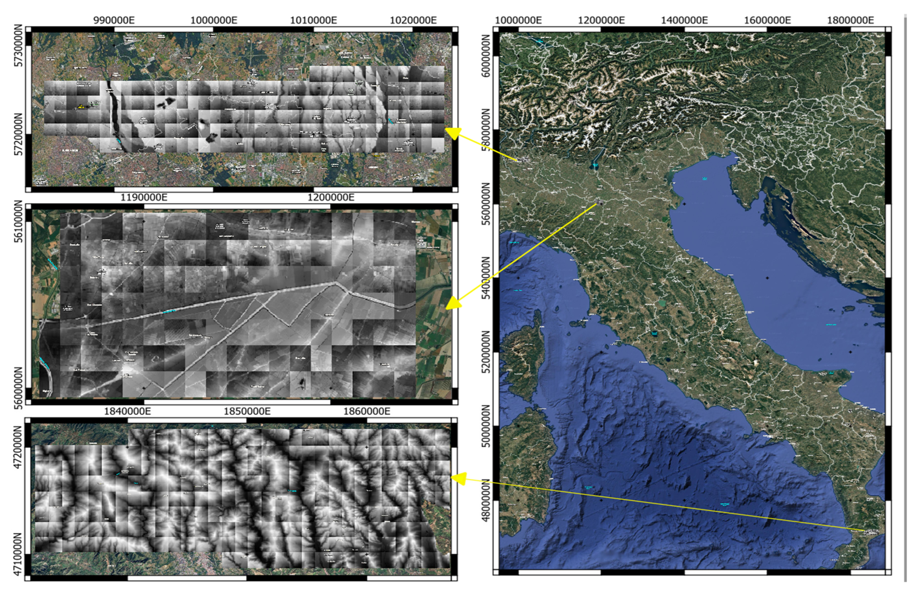
Figure 2.
Simplified RCAN-Based DTM Super Resolution workflow.
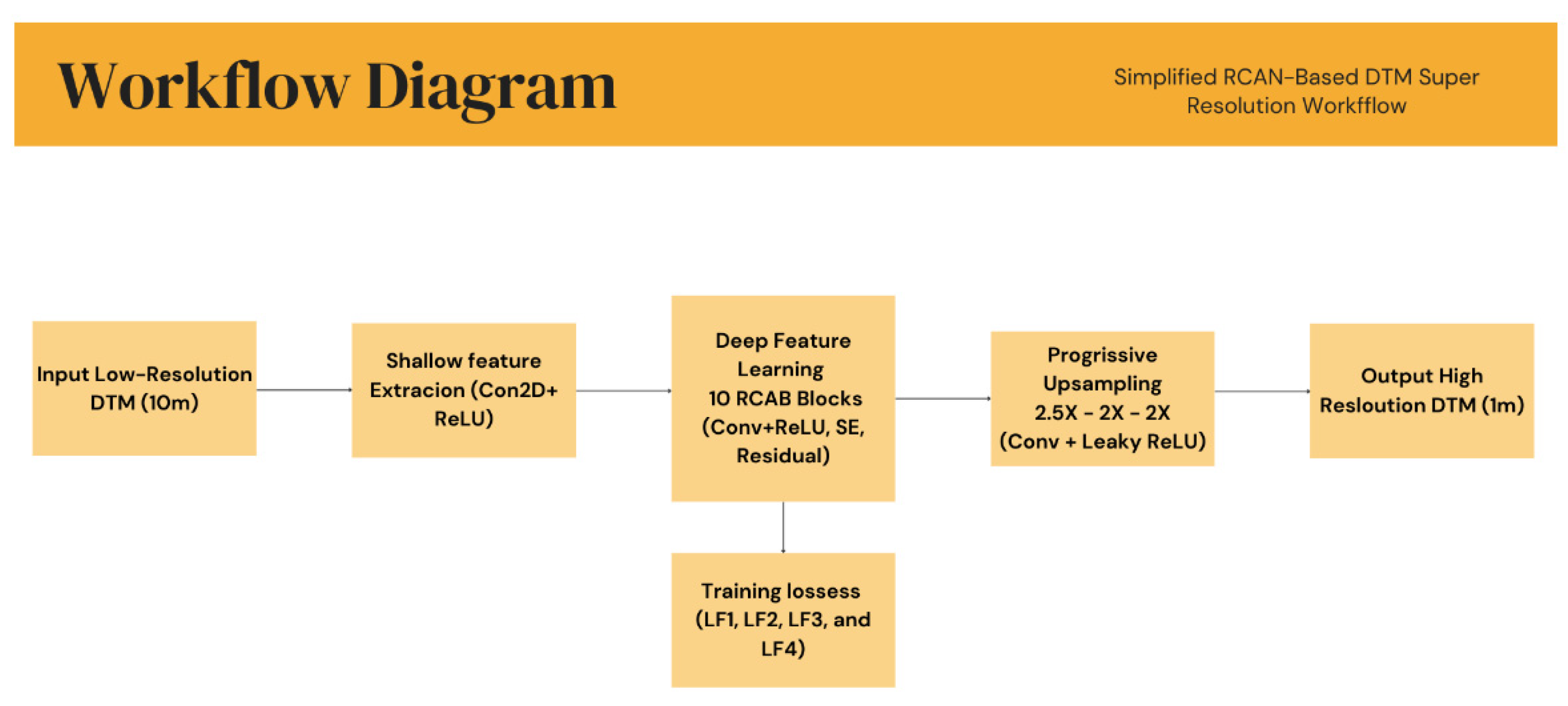
Figure 3.
Comparison of the generated super resolution DEMs with their ground truth for some example tiles, using LF4 loss function.
Figure 3.
Comparison of the generated super resolution DEMs with their ground truth for some example tiles, using LF4 loss function.
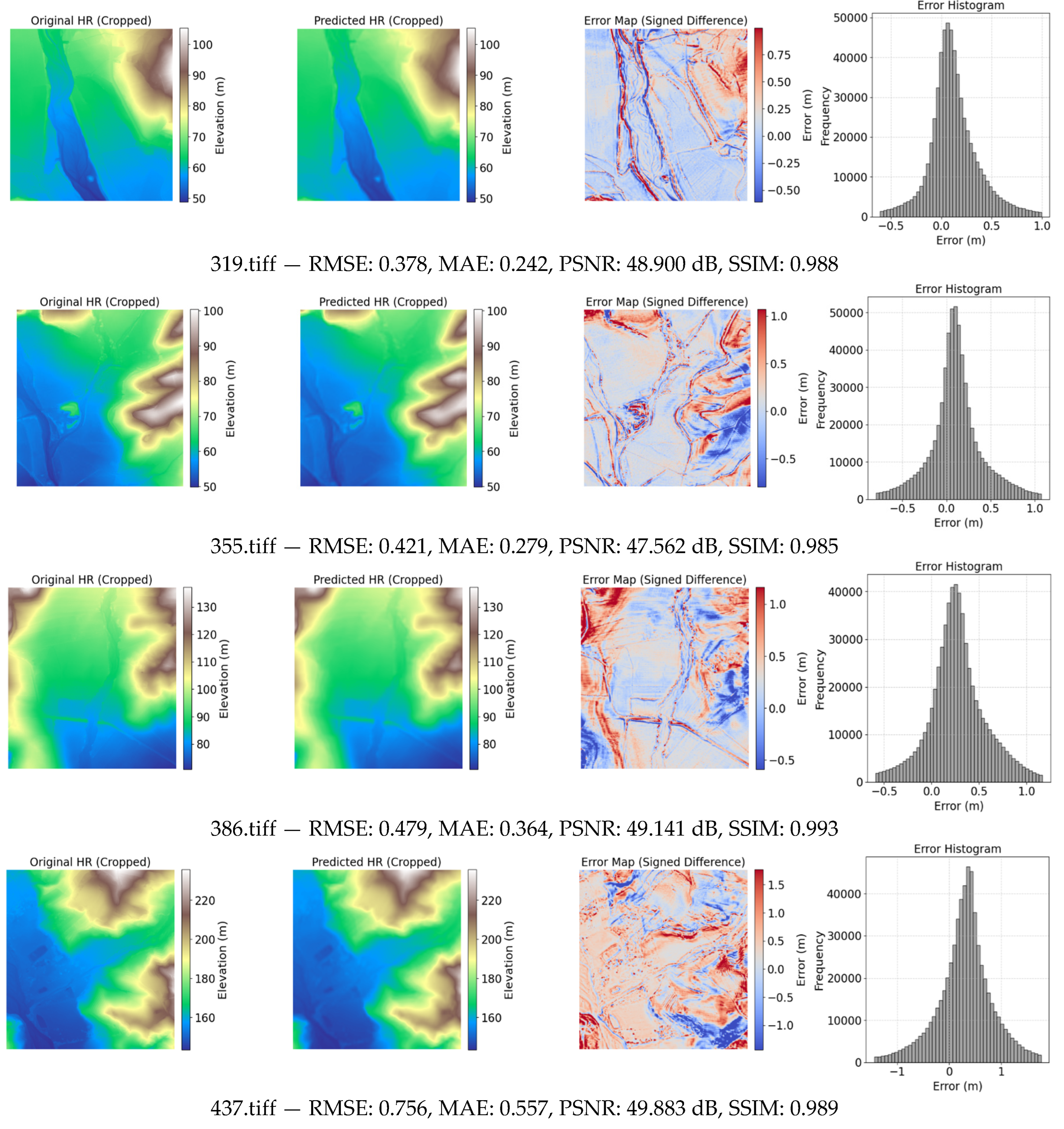
Figure 4.
visualization of the generated Super resolution samples with the ground truth tiles using LF2 loss function.
Figure 4.
visualization of the generated Super resolution samples with the ground truth tiles using LF2 loss function.
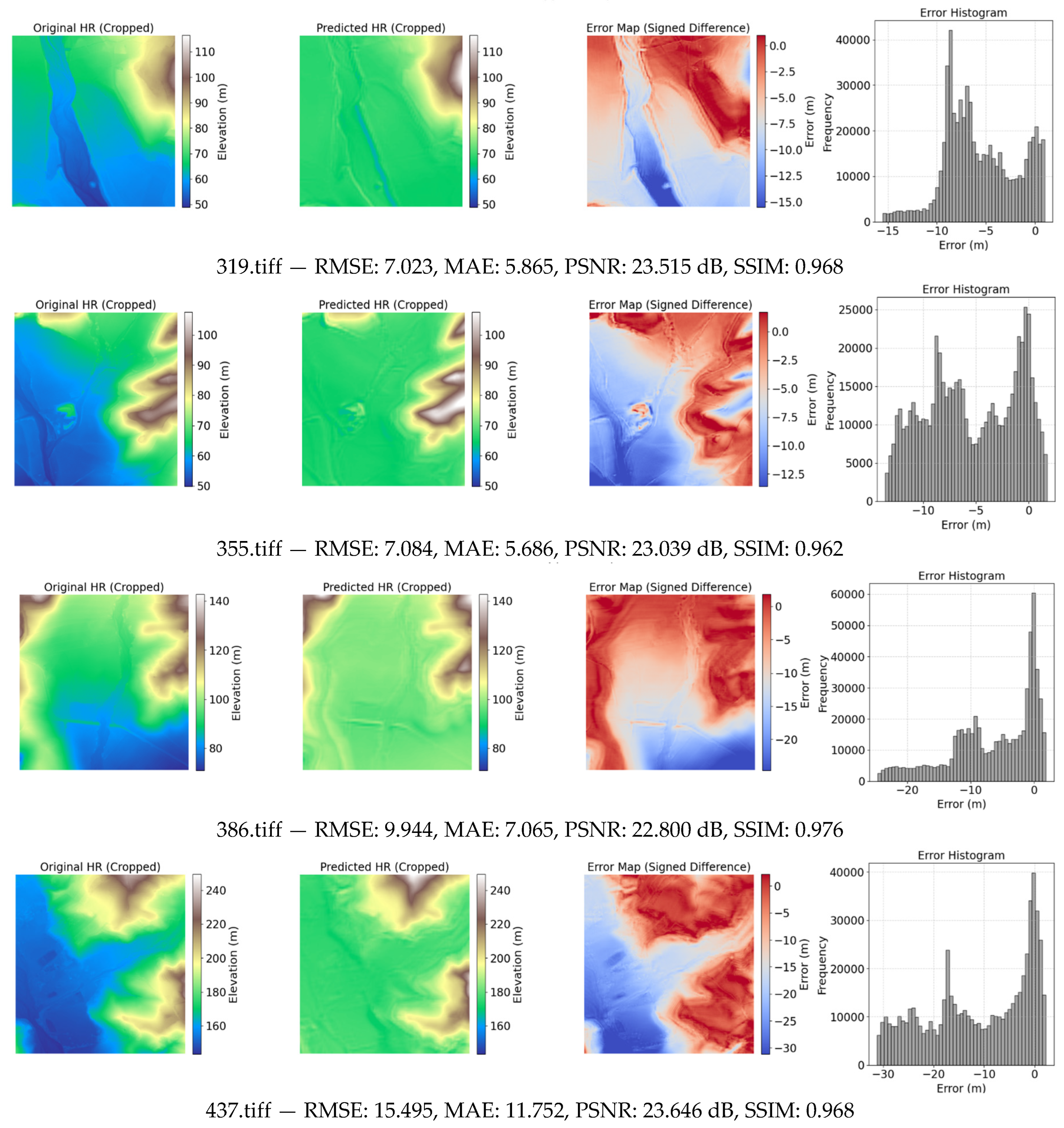
Figure 5.
performance of the four loss functions using tile-wise averaged metrics RMSE, MAE, PSNR, and SSIM.
Figure 5.
performance of the four loss functions using tile-wise averaged metrics RMSE, MAE, PSNR, and SSIM.
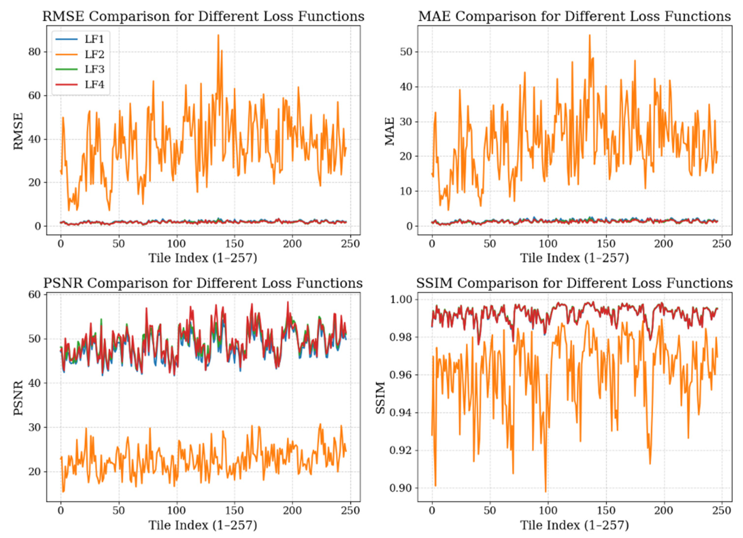
Figure 6.
visualization of the generated Super resolution samples with the ground truth tiles using fine tuning (α=0.8, γ=0.2) of LF4 loss function.
Figure 6.
visualization of the generated Super resolution samples with the ground truth tiles using fine tuning (α=0.8, γ=0.2) of LF4 loss function.
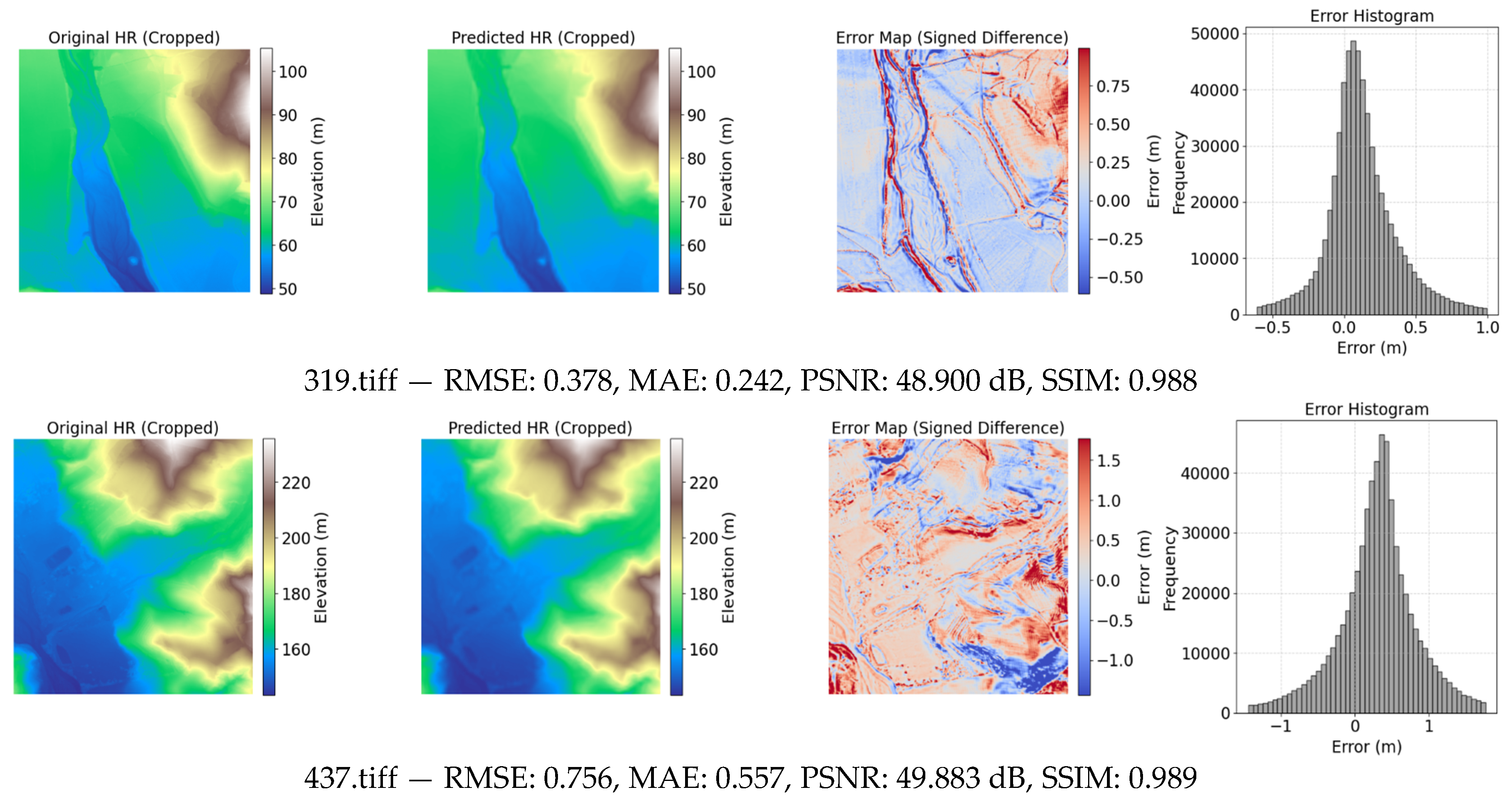
Figure 7.
visualization of the generated Super resolution samples with the ground truth tiles using fine tuning (α=0.5, γ=0.5) of LF4 loss function.
Figure 7.
visualization of the generated Super resolution samples with the ground truth tiles using fine tuning (α=0.5, γ=0.5) of LF4 loss function.
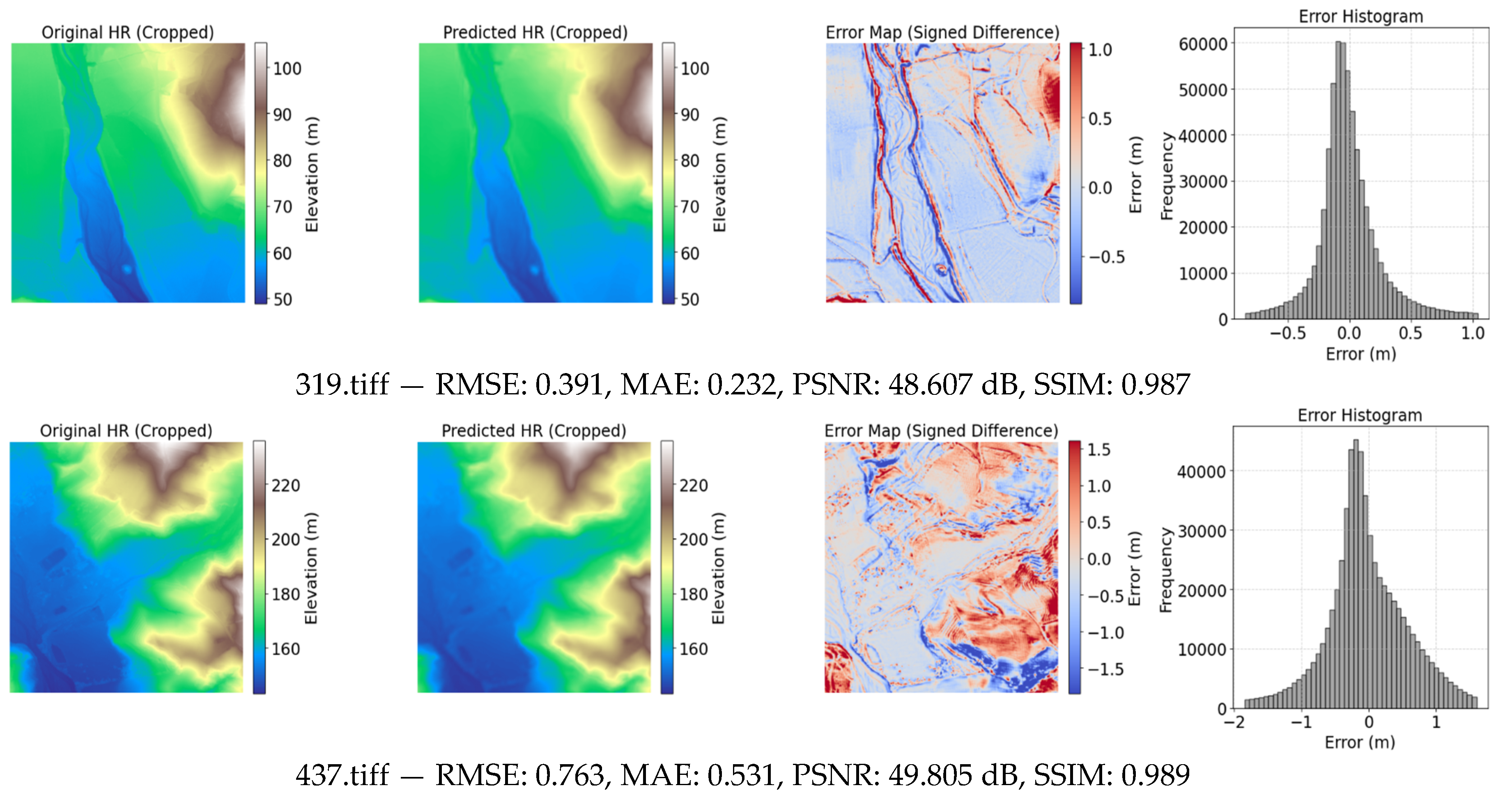
Figure 8.
visualization of the generated Super resolution samples with the ground truth tiles using fine tuning (α=0.2, γ=0.8) of LF4 loss function.
Figure 8.
visualization of the generated Super resolution samples with the ground truth tiles using fine tuning (α=0.2, γ=0.8) of LF4 loss function.
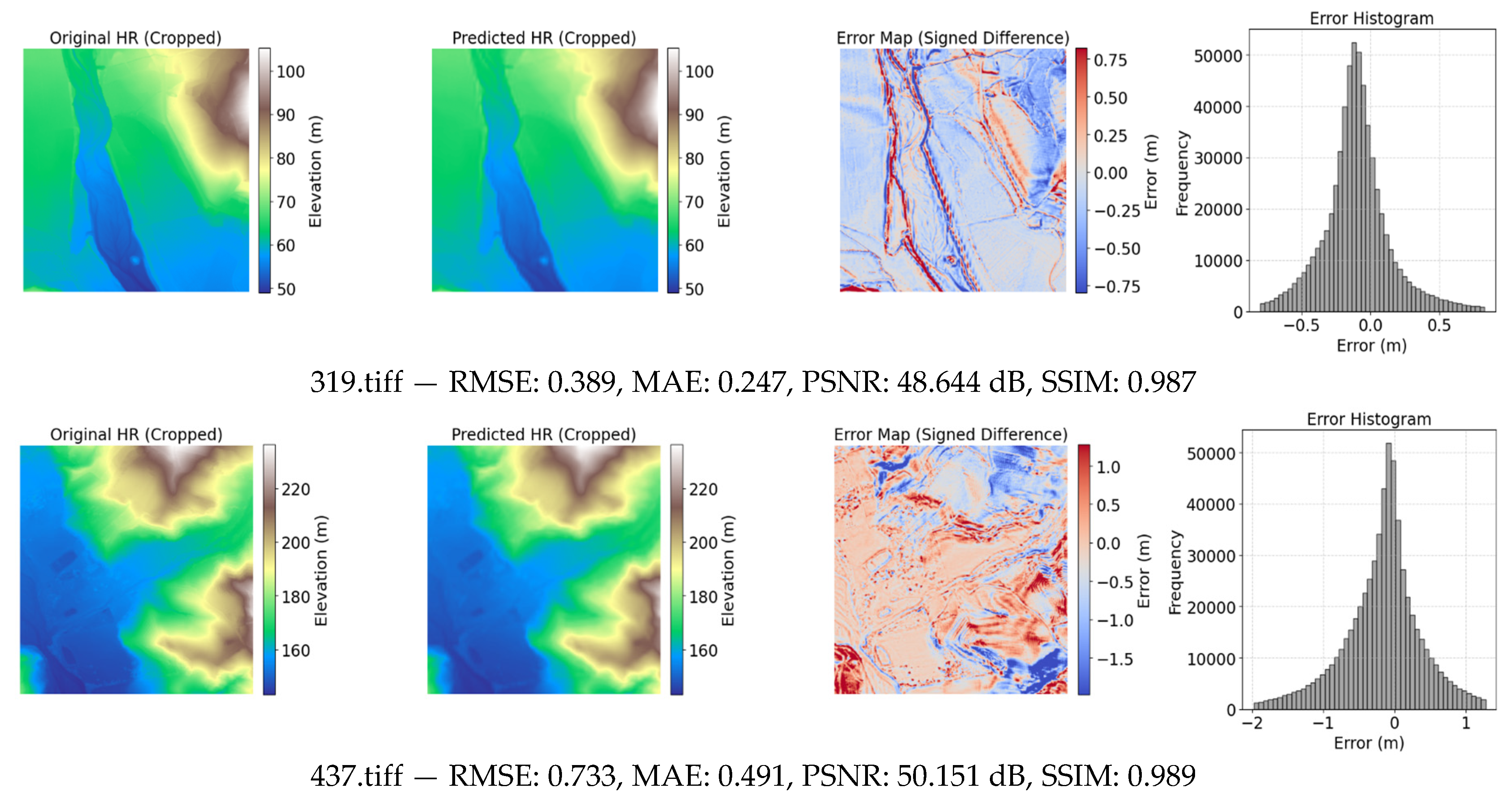
Figure 9.
performance of the three-fine tuning of LF4 A) (α=0.8, γ=0.2), B) (α=0.5, γ=0.5), and C) (α=0.2, γ=0.8) using tile-wise averaged metrics RMSE, MAE, PSNR, and SSIM.
Figure 9.
performance of the three-fine tuning of LF4 A) (α=0.8, γ=0.2), B) (α=0.5, γ=0.5), and C) (α=0.2, γ=0.8) using tile-wise averaged metrics RMSE, MAE, PSNR, and SSIM.
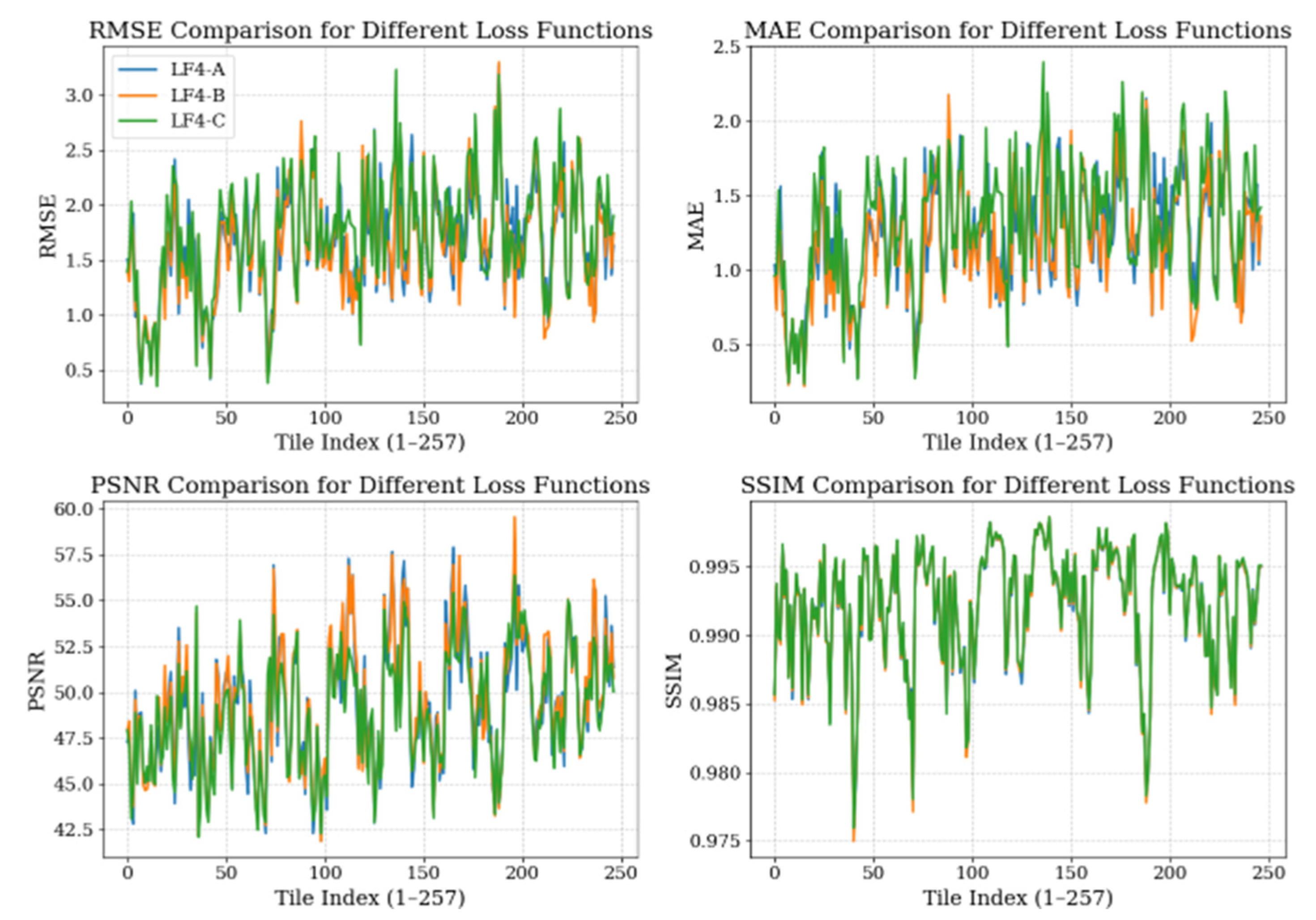
Figure 10.
MAE distribution for Four loss functions.
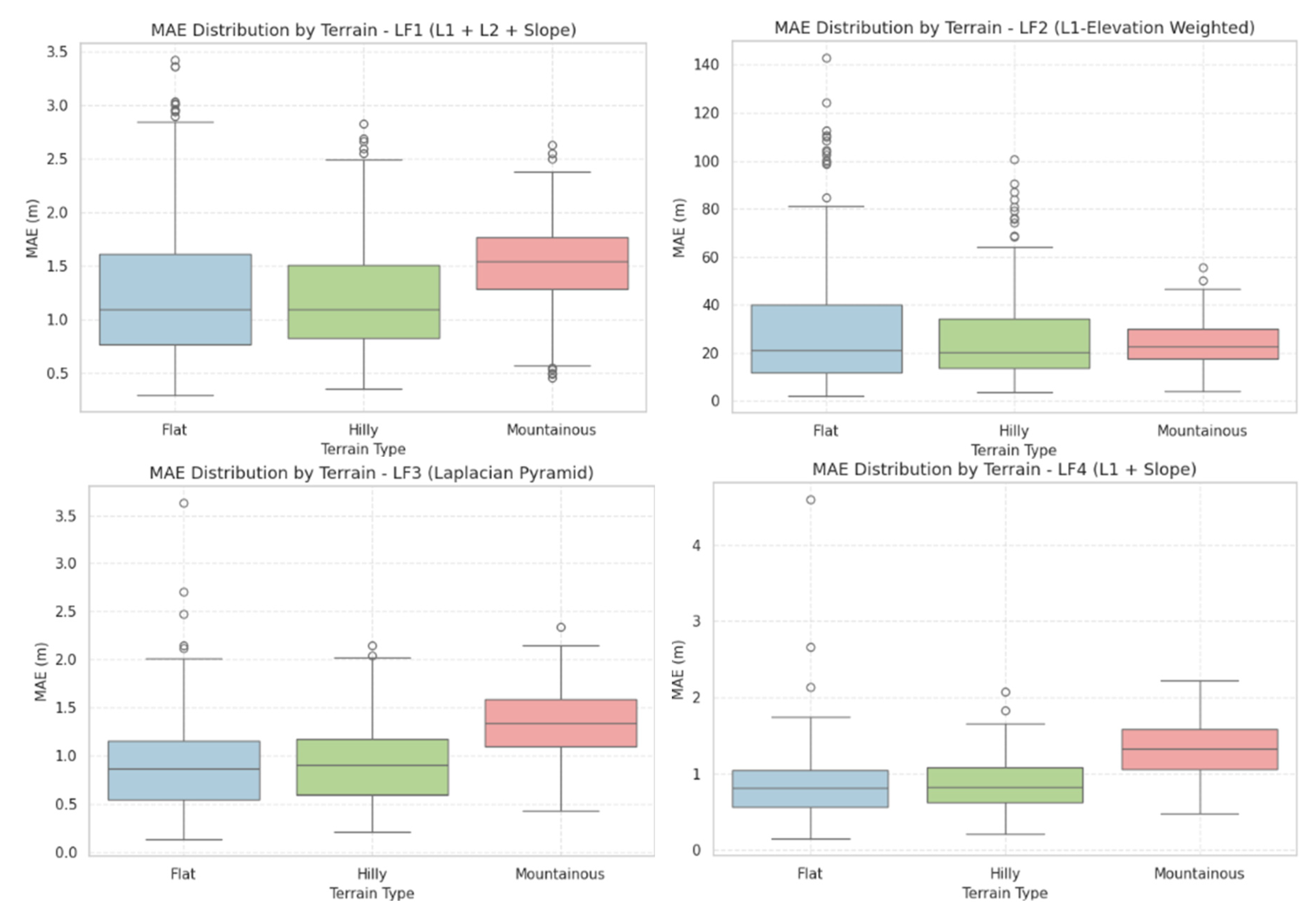
Figure 11.
RMSE distribution for Four loss functions.
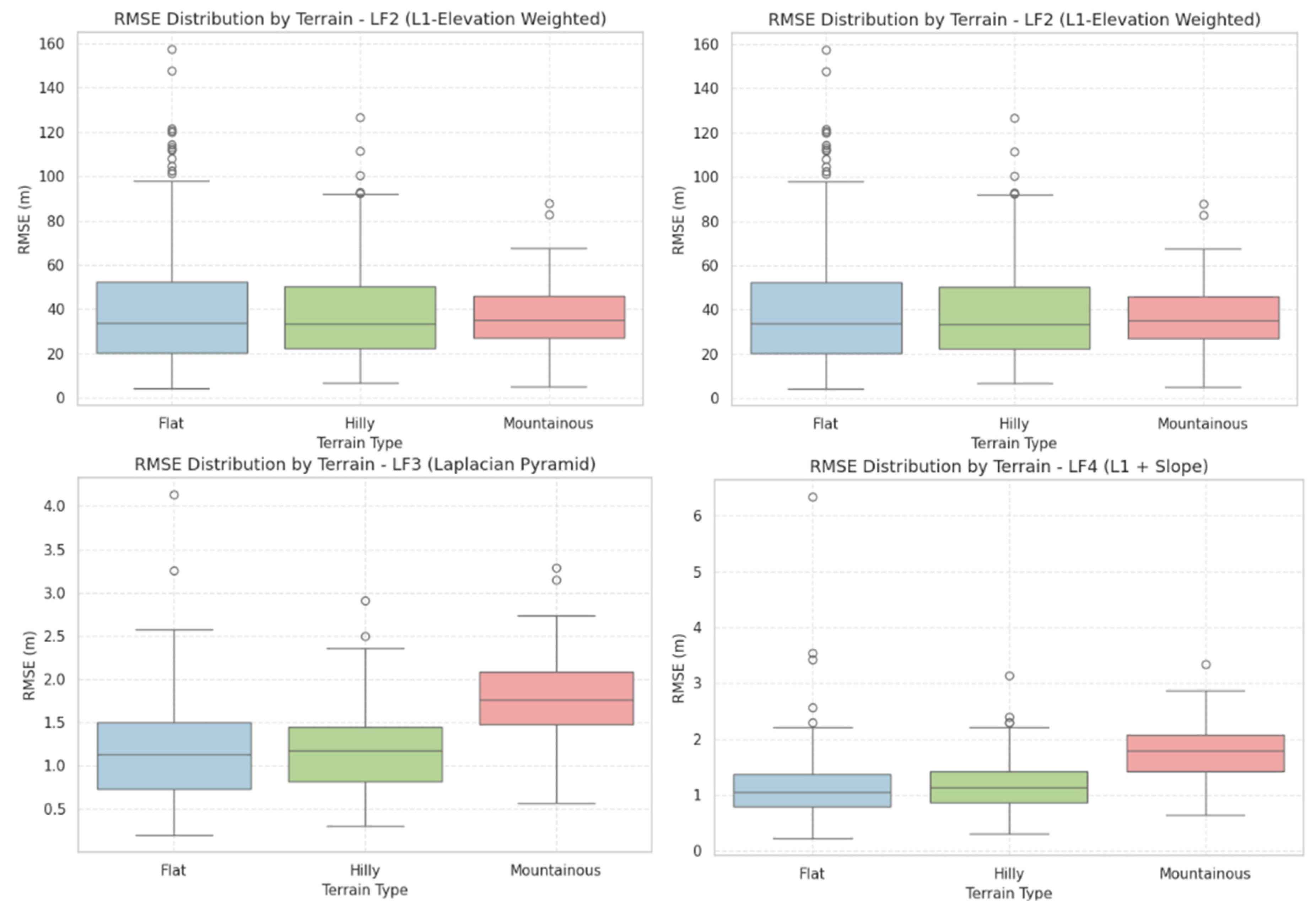
Figure 12.
Bais distribution for Four loss functions.
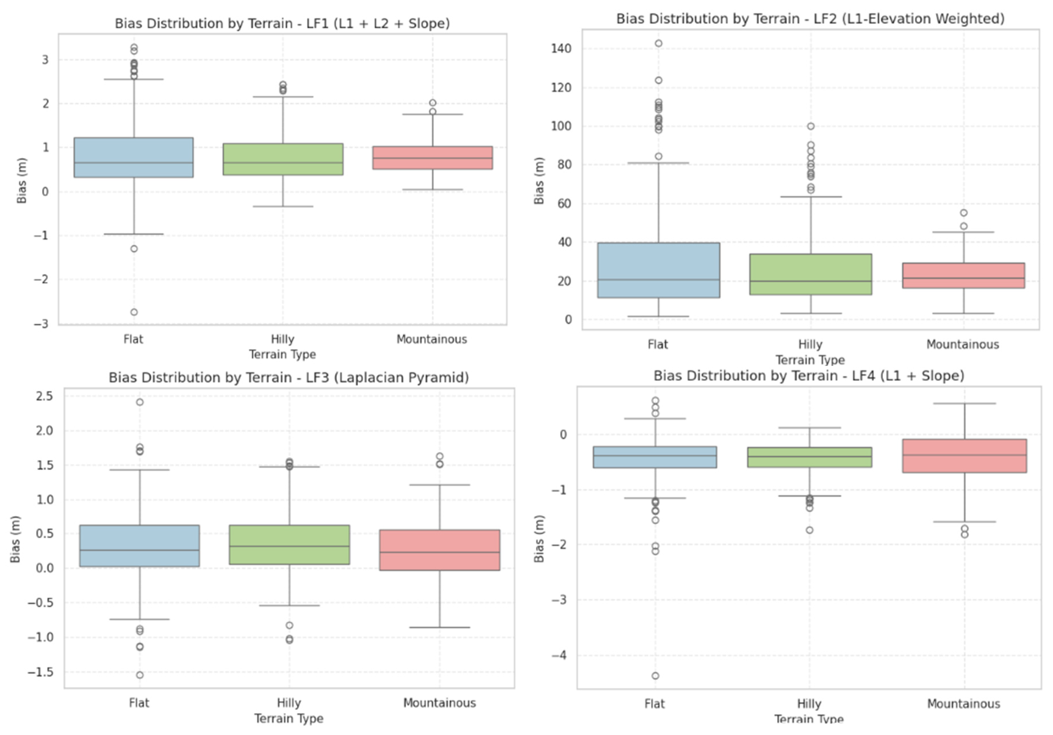
Figure 13.
MAE distribution for Fine tuning.
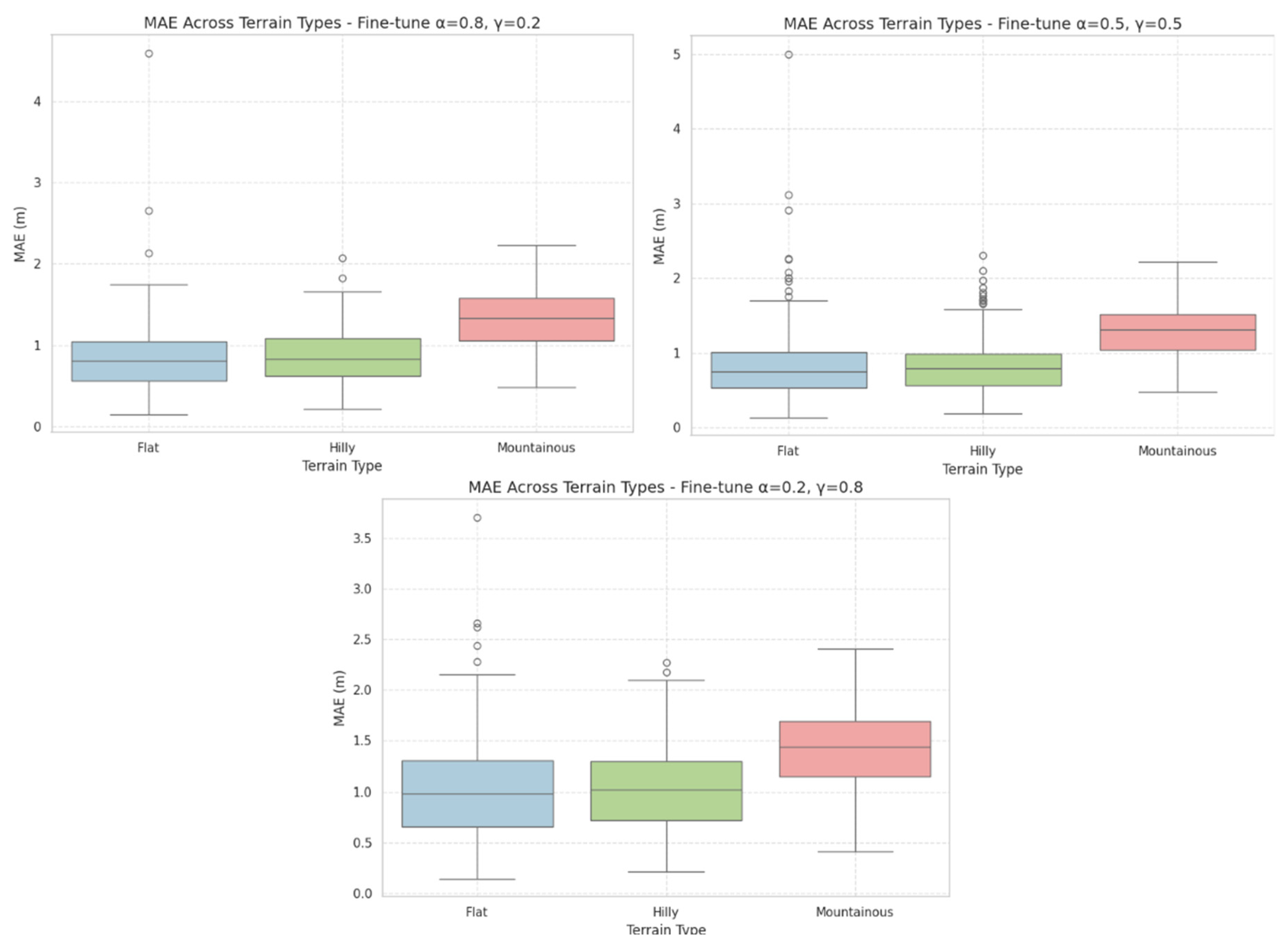
Figure 14.
RMSE distribution for Fine tuning.
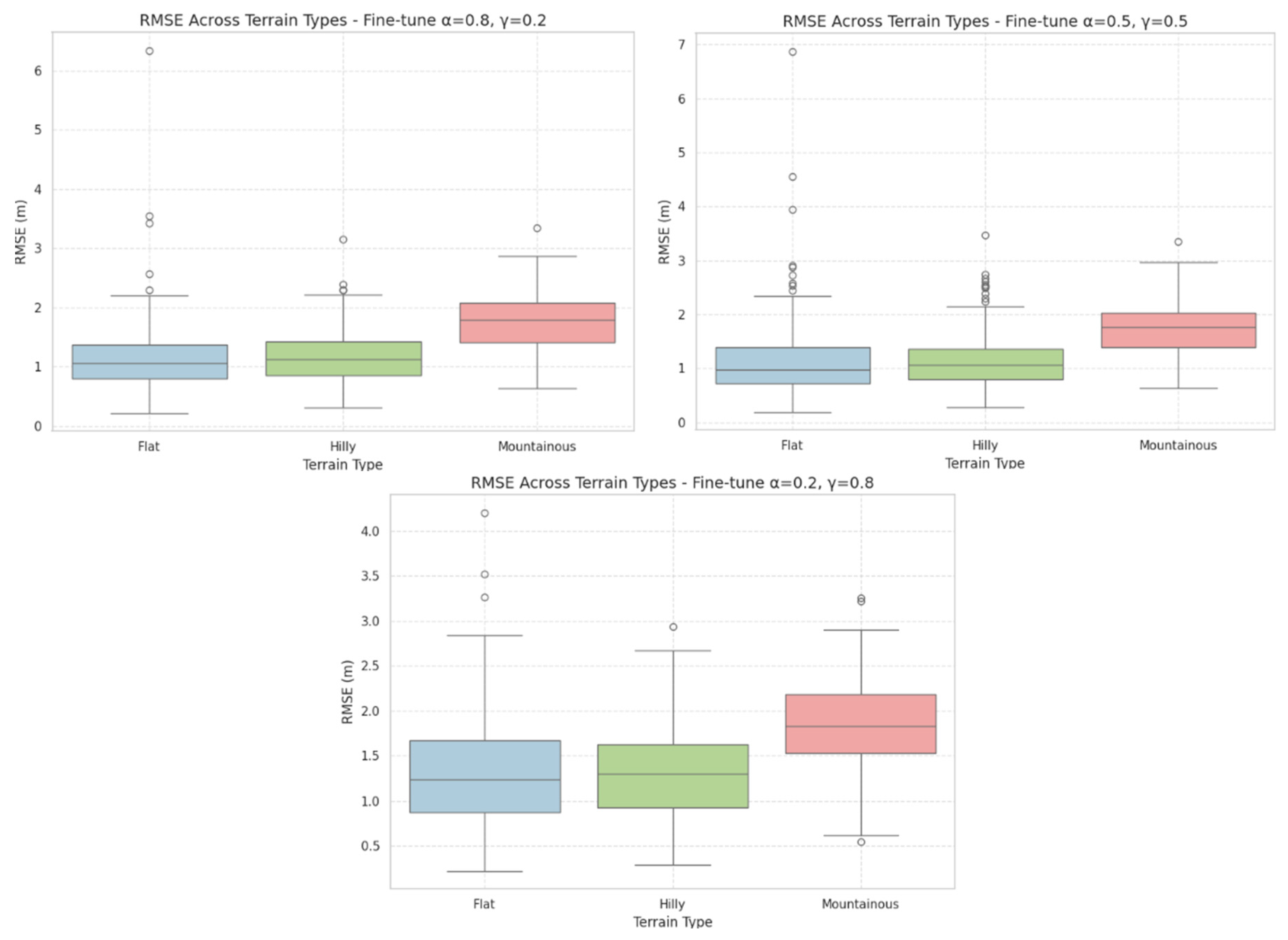
Figure 15.
Bais distribution for Fine tuning.
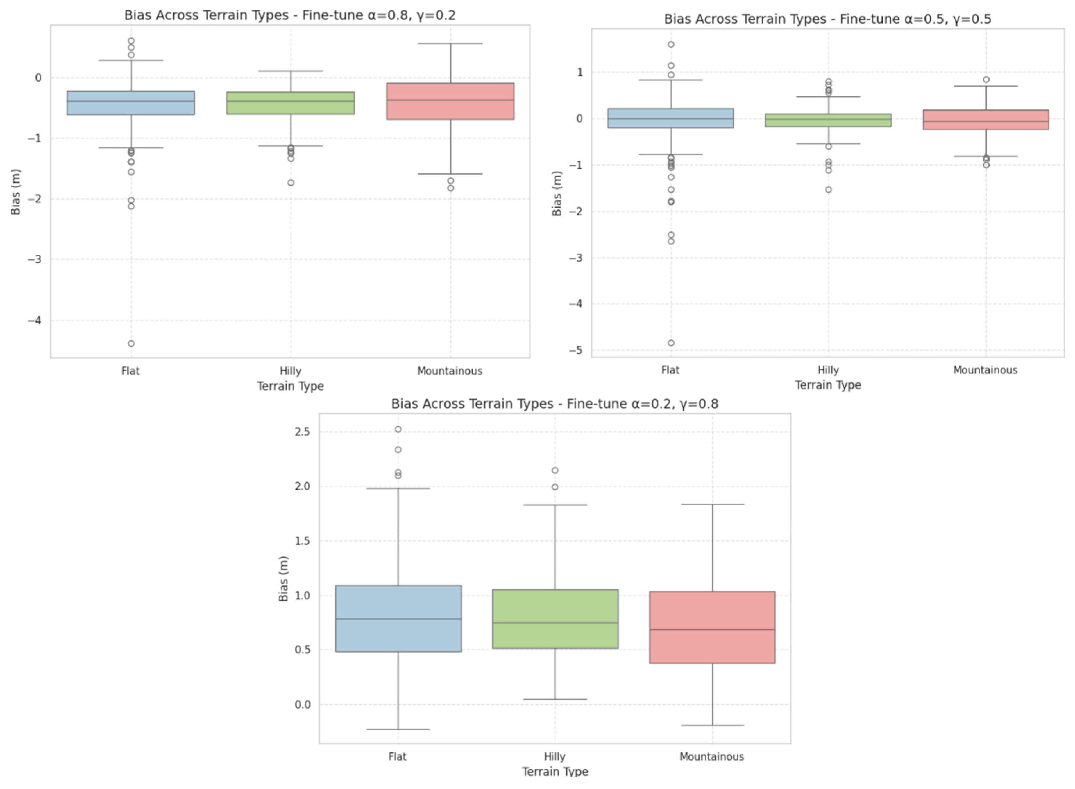
Figure 16.
the training loss curves for the model trained with the four loss functions.
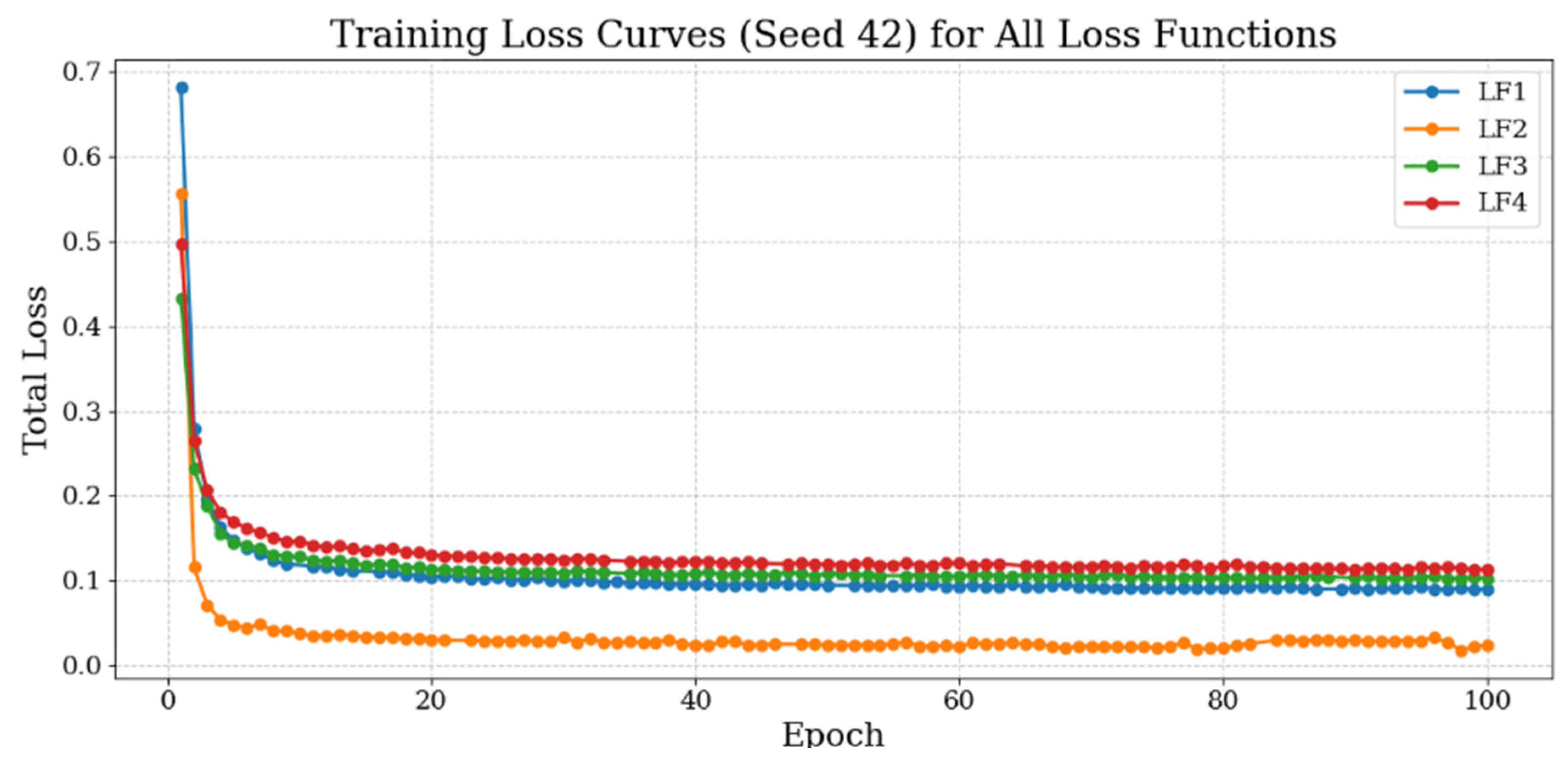
Figure 17.
the training loss curves for the model trained with A) (α=0.8, γ=0.2), B) (α=0.5, γ=0.5), and C) (α=0.2, γ=0.8).
Figure 17.
the training loss curves for the model trained with A) (α=0.8, γ=0.2), B) (α=0.5, γ=0.5), and C) (α=0.2, γ=0.8).
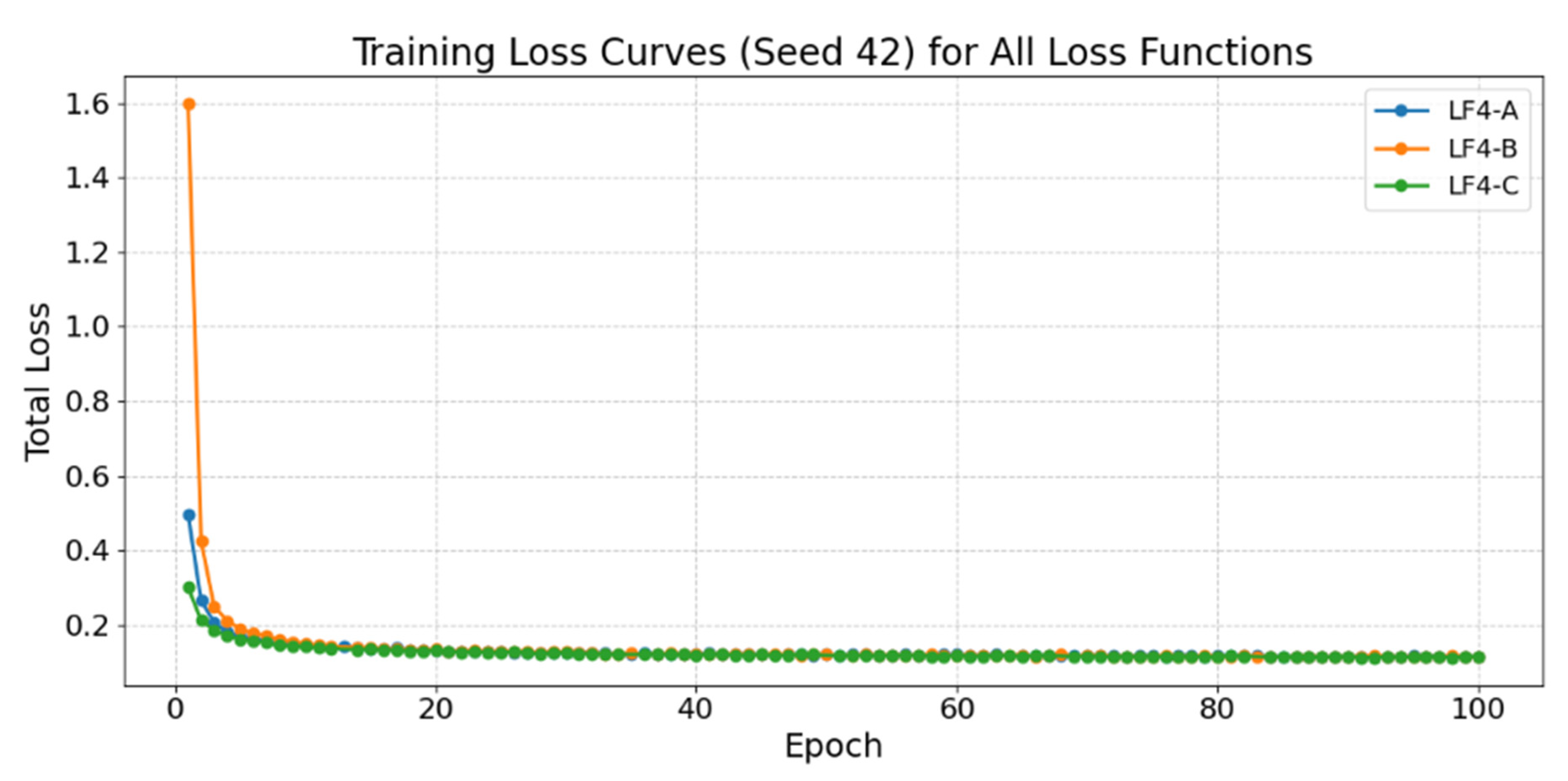

Table 1.
Quantitative results of different loss functions using RCAN Super-Resolution technique.
| loss function | LF1 | LF2 | LF3 | LF4 | ||||
|---|---|---|---|---|---|---|---|---|
| Validation | Testing | Validation | Testing | Validation | Testing | Validation | Testing | |
| Mean RMSE (M) | 0.28 | 1.90 ± 0.54 | 2.82 | 36.84 ± 13.99 | 0.27 | 1.66 ± 0.49 | 0.28 | 1.64 ± 0.49 |
| MAE (M) | _ | 1.45 ± 0.43 | _ | 24.14 ± 9.44 | _ | 1.23 ± 0.39 | _ | 1.21 ± 0.38 |
| Mean PSNR(dB) | 59.43 | 48.01 ± 3.02 | 40.34 | 22.59 ± 3.08 | 59.74 | 49.24 ± 3.14 | 59.47 | 49.30 ± 3.49 |
| Mean SSIM (M) | 0.94 | 0.99 ± 0.01 | 0.90 | 0.96 ± 0.01 | 0.94 | 0.99 ± 0.01 | 0.94 | 0.99 ± 0.01 |
Table 2.
summarizing of statistical results of the three fine tuning combination of LF4 loss function.
Table 2.
summarizing of statistical results of the three fine tuning combination of LF4 loss function.
| loss function | (α=0.8, γ=0.2) | (α=0.5, γ=0.5) | (α=0.2, γ=0.8) | |||
|---|---|---|---|---|---|---|
| Validation | Testing | Validation | Testing | Validation | Testing | |
| Mean RMSE (M) | 0.28 | 1.64 ± 0.49 | 0.28 | 1.62 ± 0.50 | 0.28 | 1.73 ± 0.52 |
| MAE (M) | - | 1.21 ± 0.38 | - | 1.18 ± 0.39 | - | 1.32 ± 0.42 |
| Mean PSNR (dB) | 59.47 | 49.30 ± 3.49 | 59.52 | 49.47 ± 3.50 | 59.44 | 48.88 ± 3.10 |
| Mean SSIM (M) | 0.94 | 0.99 ± 0.01 | 0.94 | 0.99 ± 0.01 | 0.94 | 0.99 ± 0.01 |
Table 3.
slope-based zonal statistics assessment for different loss functions.
| Model | Terrain | Mean MAE (m) | Mean RMSE (m) | Mean Bias (m) |
|---|---|---|---|---|
| LF1 | Flat | 1.27 | 1.62 | +0.82 |
| Hilly | 1.21 | 1.57 | +0.78 | |
| Mountainous | 1.52 | 1.99 | +0.77 | |
| LF2 | Flat | 30.14 | 40.85 | +29.76 |
| Hilly | 26.36 | 38.50 | +25.90 | |
| Mountainous | 23.57 | 35.94 | +22.68 | |
| LF3 | Flat | 0.90 | 1.16 | +0.32 |
| Hilly | 0.91 | 1.19 | +0.34 | |
| Mountainous | 1.33 | 1.77 | +0.26 | |
| LF4 | Flat | 0.85 | 1.15 | –0.47 |
| Hilly | 0.86 | 1.17 | –0.43 | |
| Mountainous | 1.32 | 1.76 | –0.41 |
Table 4.
slope based zonal statistics assessment for different fine-tuning for LF4 loss function.
| Model | Terrain | Mean MAE (m) | Mean RMSE (m) | Mean Bias (m) |
|---|---|---|---|---|
| α=0.8, γ=0.2 | Flat | 0.85 | 1.15 | –0.47 |
| Hilly | 0.86 | 1.17 | –0.43 | |
| Mountainous | 1.32 | 1.76 | –0.41 | |
| α=0.5, γ=0.5 | Flat | 0.83 | 1.14 | –0.04 |
| Hilly | 0.83 | 1.15 | –0.03 | |
| Mountainous | 1.29 | 1.73 | –0.04 | |
| α=0.2, γ=0.8 | Flat | 1.02 | 1.29 | +0.83 |
| Hilly | 1.03 | 1.31 | +0.80 | |
| Mountainous | 1.41 | 1.84 | +0.72 |
Disclaimer/Publisher’s Note: The statements, opinions and data contained in all publications are solely those of the individual author(s) and contributor(s) and not of MDPI and/or the editor(s). MDPI and/or the editor(s) disclaim responsibility for any injury to people or property resulting from any ideas, methods, instructions or products referred to in the content. |
© 2025 by the authors. Licensee MDPI, Basel, Switzerland. This article is an open access article distributed under the terms and conditions of the Creative Commons Attribution (CC BY) license (https://creativecommons.org/licenses/by/4.0/).
Copyright: This open access article is published under a Creative Commons CC BY 4.0 license, which permit the free download, distribution, and reuse, provided that the author and preprint are cited in any reuse.


