Submitted:
03 November 2025
Posted:
17 November 2025
You are already at the latest version
Abstract
This paper introduces a deep learning-based methodology for the automated identification of spalling defects in tunnel linings, emphasizing the fusion of intensity and depth information. A novel network architecture is presented, leveraging Mobile Laser Scanning (MLS) data to generate a dataset of paired intensity and depth images. The network effectively integrates these multi-modal inputs to enhance the precision of spalling segmentation. Results demonstrate the superior performance of the proposed approach in comparison to methods relying solely on intensity data, highlighting the critical role of depth information for accurate defect characterization in complex underground environments.
Keywords:
deep learning
; spalling defect detection
; tunnel linings
; intensity-depth fusion
1. Introduction
Over recent decades, China’s transportation network has undergone substantial growth, leading to a marked increase in the construction of railway tunnels. With prolonged usage, tunnel linings deteriorate and develop structural anomalies such as fissures, seepage, surface flaking, and distortion. Among these, surface flaking—referred to as concrete spalling—emerges as one of the most prevalent issues observed on tunnel linings. If neglected, dislodged concrete segments may pose operational hazards and financial repercussions [1].
Currently, assessments of spalling are typically conducted by trained staff who traverse the tunnel, manually recording observations. This approach introduces subjectivity and lacks quantitative detail. The limited inspection window, often confined to nocturnal hours, restricts thorough assessments and highlights the necessity for efficient, automated alternatives [2].
Vision-based automation has advanced through techniques such as photogrammetry, which utilizes photographic imagery to extract defect characteristics. However, these two-dimensional captures lack depth perception and are often compromised by environmental lighting and distance variability [3]. Alternatively, Mobile Laser Scanning (MLS), grounded in Light Detection and Ranging (LiDAR), offers consistent acquisition of spatially accurate three-dimensional point clouds, encapsulating both texture and depth characteristics [4].
Despite the integration of image processing and surface roughness metrics, conventional methods fall short in extracting semantic insights and achieving reliable defect classification [5]. Deep convolutional neural networks (DCNNs) have established superior performance in semantic segmentation tasks. Various architectures—VGG, ZFNet, GoogleNet, and ResNet—along with models such as FCN, Mask R-CNN, and YOLO, have demonstrated utility across diverse defect detection tasks [6,7].
Nevertheless, distinguishing spalling within complex tunnel visuals remains challenging due to lighting inconsistencies and obstructive elements. RGB-based datasets, lacking depth, often hinder the DCNNs’ precision. Integrating RGB imagery with depth data (RGB-D) enhances detection performance by capturing the spatial relationship between surfaces and defects [8].
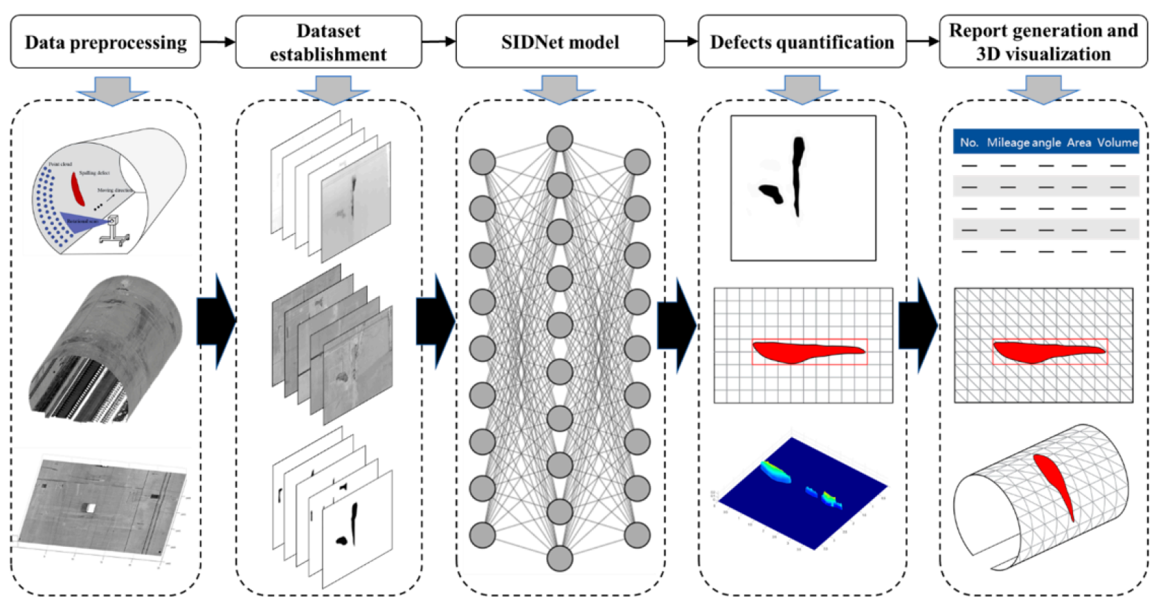
To date, few studies have explored spalling detection using combined color and depth information. This research introduces a novel framework leveraging MLS-acquired depth and intensity data integrated with a DCNN architecture, termed Spalling Intensity Depurator Network (SIDNet). The proposed system executes spalling detection and measurement in an automated manner and reconstructs 3D visualizations using triangulated meshes.
Figure 1.
Overview of the proposed methodology for spalling defect detection and analysis.
2. Data Acquisition and Dataset Development
2.1. Three-Dimensional Point Cloud Collection
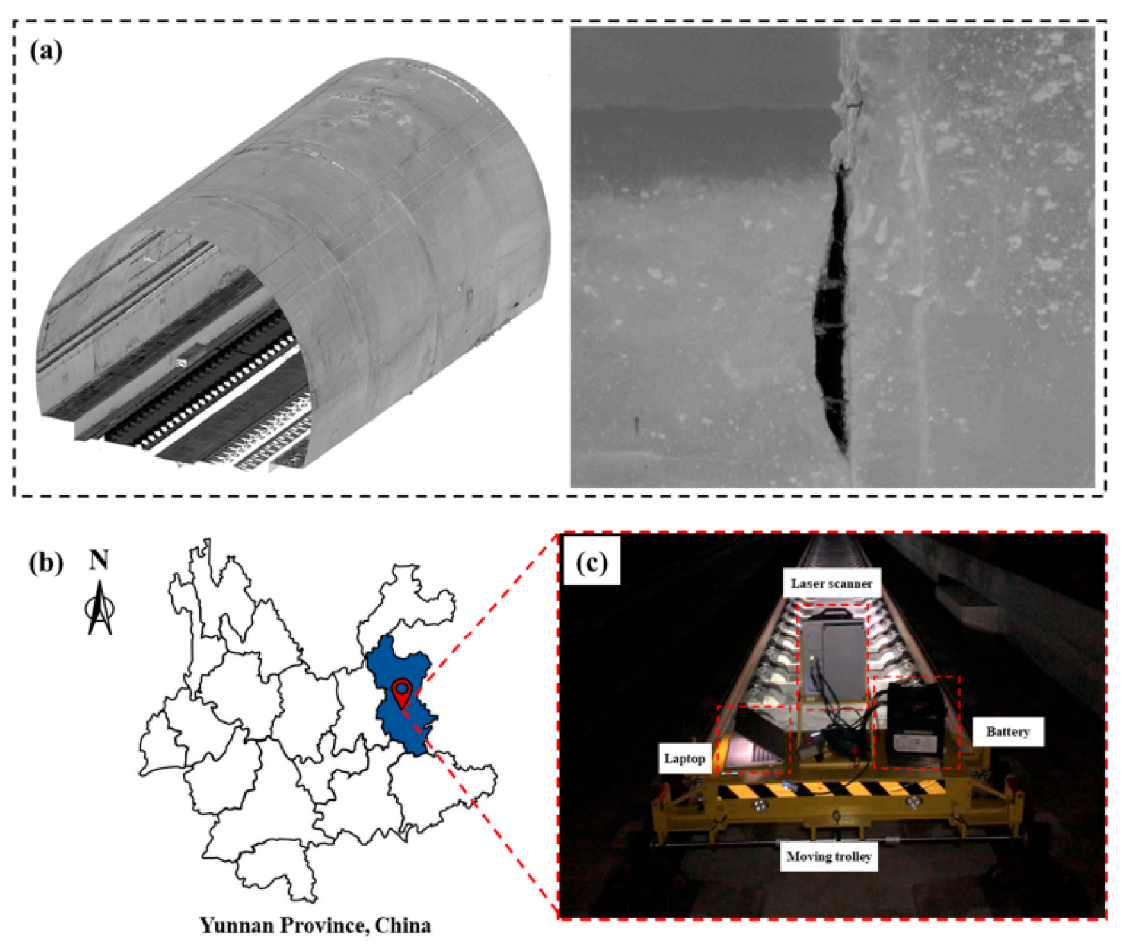
To extract both geometric structure and defect depth features, an integrated MLS configuration was employed in railway tunnels within Yunnan Province, China. The system included a Z+F PROFILER 9012 scanner mounted on a motorized platform, along with power sources and control hardware.
Given the linear nature of tunnels, spatial data was acquired by moving the platform along the railway. Operations were restricted to midnight through 4 a.m. to avoid service disruptions. Over a two-week period, data encompassing over 25 kilometers across 22 tunnels was accumulated, totaling 120 GB.
Each scan produced precise three-dimensional coordinates paired with intensity values, forming a four-column matrix . The scanner rotated at 100 revolutions per second, while the trolley moved at a fixed rate of . Each second, 100 transverse scan lines were generated. Given these parameters, the interval between adjacent scan lines was derived using:
where v is the trolley’s velocity and f is the scanner’s rotational frequency.
Figure 2.
MLS system mounted on mobile trolley for tunnel data capture.
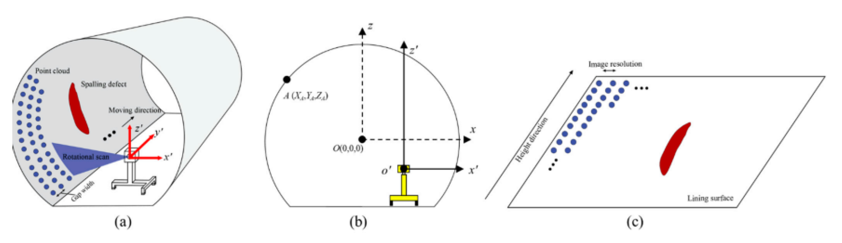
2.2. Generation of Intensity and Depth Representations
The captured point cloud data, organized along identical longitudinal positions (Y), was projected onto a 2D plane. To counteract radial distortion, coordinate transformation centered around the tunnel’s elliptical cross-section was performed using RANSAC and ellipse-fitting algorithms.
Subsequently, greyscale images were generated from the intensity values. Each scan line was treated as a horizontal row in a matrix, and the point-wise intensity I values were mapped to greyscale levels within an 8-bit range (0–255). Longitudinal and transverse resolutions were uniformly set at .
To determine depth, the Euclidean distance between each point and the fitted ellipse surface was calculated:
where R is the radial distance to the fitted ellipse.
To improve visual clarity, a power-law transformation was applied to the depth values, producing enhanced depth images:
where was empirically set to 4. This conversion darkens spalling regions and assigns mid-range values to intact surfaces.
Figure 3.
Depth image conversion process with interference region interpolation.
Obstructions such as cables were assigned maximum pixel values (white), which hindered segmentation accuracy. Linear interpolation was employed to estimate hidden depths behind such objects, ensuring continuity in spalling defect measurement.
3. Dataset Preparation for Spalling Analysis
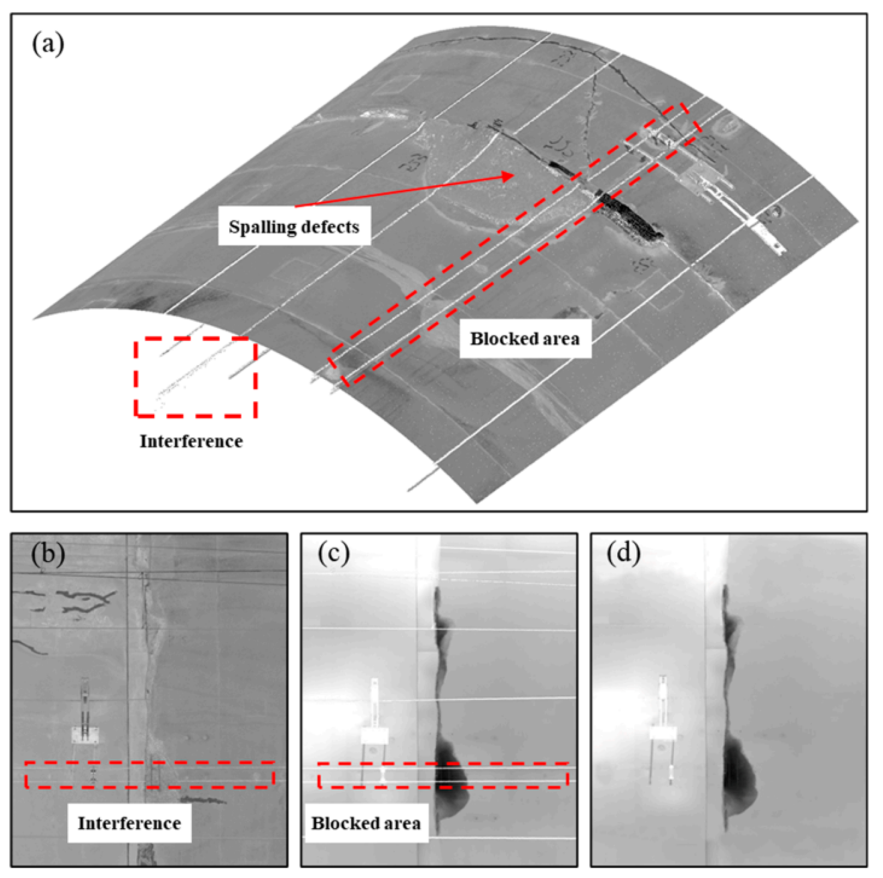
To facilitate the identification of surface degradation, a dataset incorporating both intensity and depth modalities, named Railway Tunnel Surface Damage (RTSD), is compiled. Each original frame indicating damage is resized by cropping, during which corner coordinates are retained to ensure consistent processing across modalities. This uniform cropping is implemented via an algorithm that maintains spatial alignment between the intensity and depth views.
Figure 4.
Eliminating interference: (a) tunnel point cloud; (b) intensity visualization; (c) raw depth image with interference; (d) refined depth image post-interference removal.
Figure 4.
Eliminating interference: (a) tunnel point cloud; (b) intensity visualization; (c) raw depth image with interference; (d) refined depth image post-interference removal.
The annotated ground truth (GT) labels, generated using the LabelMe tool, rely on comprehensive information from both visual modalities. The initial dataset includes 1156 paired depth and intensity samples. To counterbalance the limited number of defective samples, multiple augmentation strategies such as mirror flips, spatial zooming, elastic warping, and brightness variation are employed. Consequently, the expanded dataset encompasses 8092 images per modality, alongside the corresponding GT masks.
Figure 5.
RTSD dataset samples: (a) prominent depth spalling; (b) minor depth surface erosion.
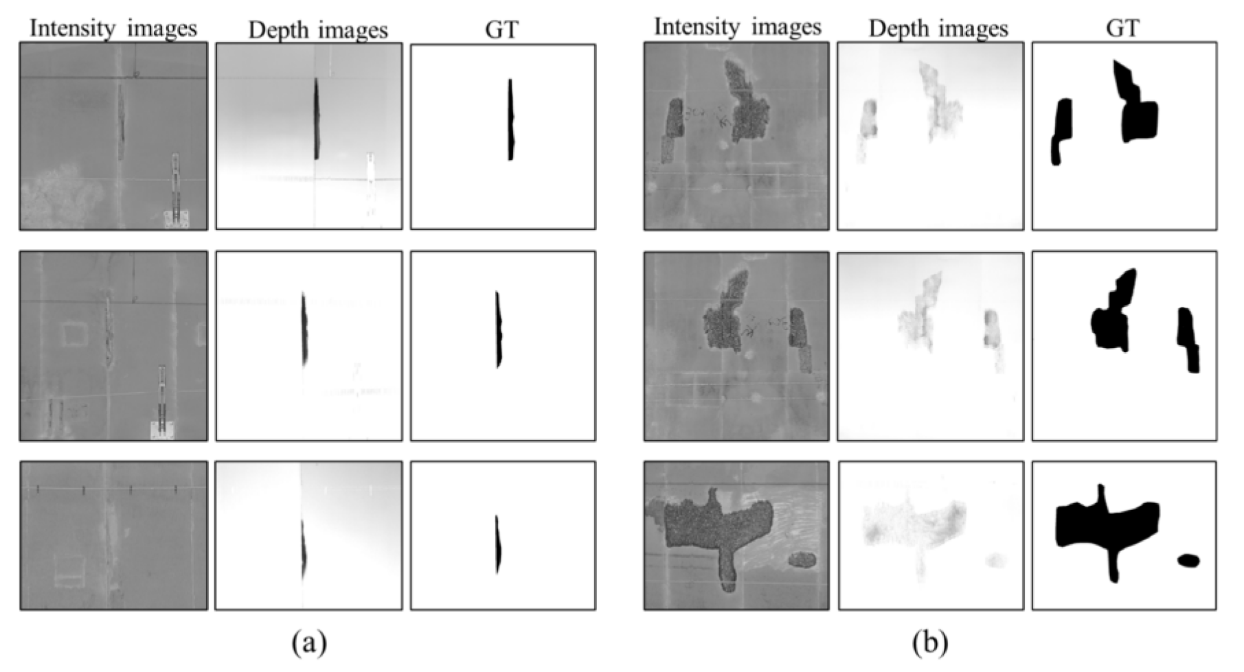
While the depth maps convey spatial depth through grayscale values, the intensity frames lack such metric information. In cases where damage is shallow, enhancements via surface treatment like resin overlay may enhance detection in intensity images. Therefore, both modalities play complementary roles in accurate surface defect assessment. The dataset’s primary advantage lies in delivering depth-aware annotations absent in traditional visual-only repositories.
4. SIDNet Architecture for Defect Segmentation
Leveraging the RTSD repository, an enhanced DCNN framework titled Spalling Intensity-Depth Network (SIDNet) is presented for automated damage segmentation. This architecture, adapted from D3Net, comprises two functional units: a triple-path feature extraction segment and an intensity filtering module.
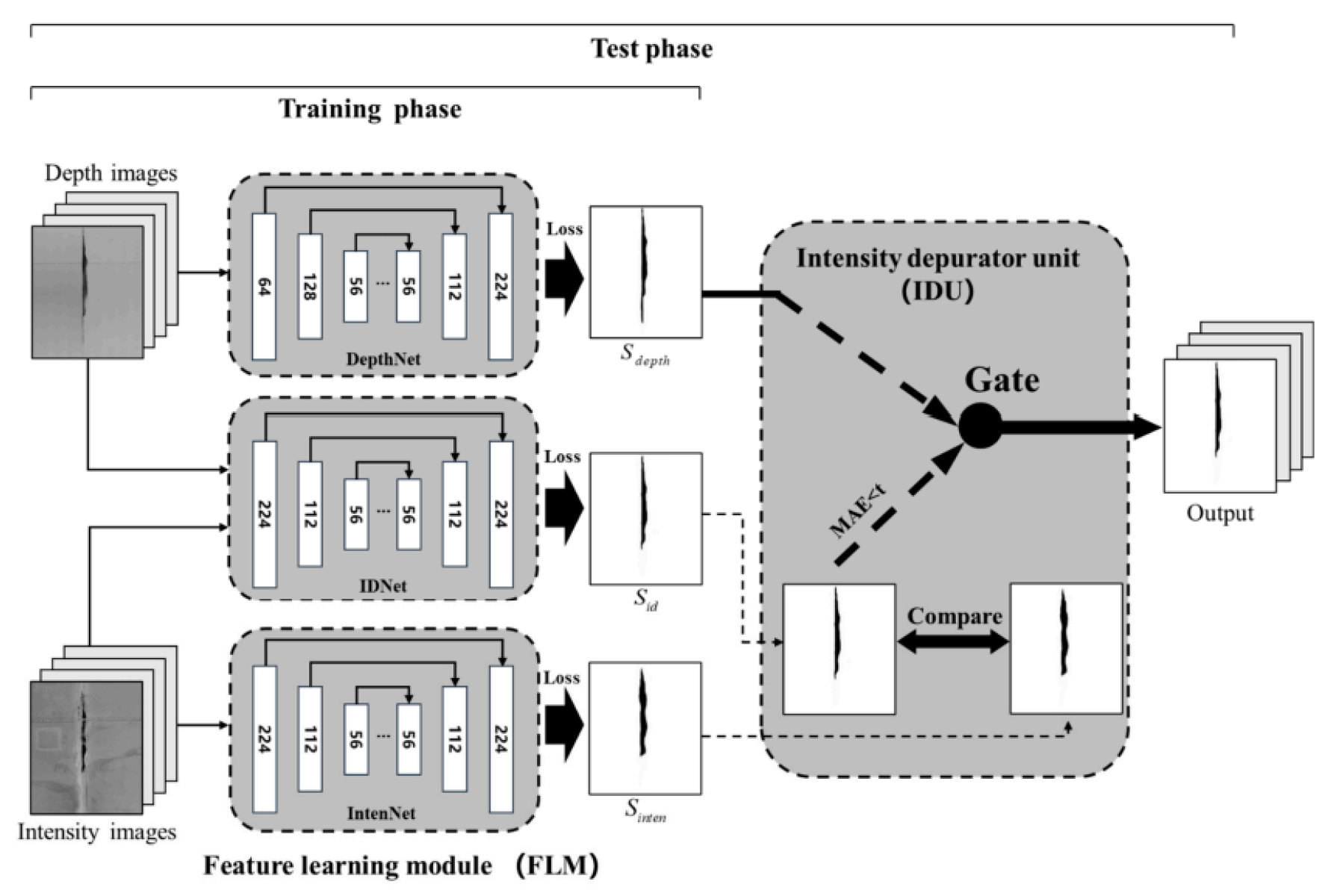
The feature extraction segment, termed the Feature Learning Module (FLM), consists of three independent encoder-decoder paths labeled IntenNet, IDNet, and DepthNet. Each path processes a distinct modality—intensity-only, combined (intensity + depth), and depth-only—using the same architectural design but different input channels.
Each model accepts inputs resized to with channel configurations of 1, 2, and 1, respectively. The outputs include predictions from each path: , , and . The FLM outputs are fed into a refinement unit for enhanced accuracy during testing.
Figure 6.
Overview of the SIDNet model featuring dual-phase operation: training and testing.
4.1. Feature Extraction Details
The core encoding process is inspired by the VGG16 structure and enhanced with a sixth convolutional block using filters. Feature maps from successive convolutional stages are , , , , , and finally .
Feature pyramid principles guide multi-scale fusion. Up-sampling through nearest-neighbor interpolation allows higher resolution restoration. Each decoder produces output via a convolution.
The loss function used for training is the binary cross-entropy loss:
where and denote GT and predicted pixel values, respectively.
4.2. Intensity Quality Filtering Module
To compensate for noisy intensity data, the Intensity Depurator Unit (IDU) filters predictions by measuring the mean absolute error (MAE) between and :
The final output P is determined by thresholding this MAE:
Comparatively, a depth filter module from D3Net, which uses and a threshold , serves a similar role but for depth image reliability.
4.3. Performance Metrics
Segmentation quality is assessed via Mean Pixel Accuracy (MPA) and Mean Intersection over Union (MIoU). Let TP, FP, TN, and FN denote true/false positives and negatives. The metrics are defined as:
Figure 7.
Correlation diagram of classification outcomes: TP, TN, FP, and FN.

4.4. Quantifying Surface Damage
Upon segmentation, spalling regions are discerned by associating pixel depth values with the reference surface, reversing the transformation process used in depth projection. The defect area is calculated as:
where is the real-world area per pixel (e.g., 25 mm2) and n is the number of identified defective pixels. Volume estimation follows by incorporating per-pixel depth differentials.
5. Experimentation and Outcomes
Prior to the model development stage, the RTSD dataset underwent a randomized segmentation into three distinct subsets—namely training, validation, and testing—comprising 70%, 20%, and 10% of the total samples, respectively. The image allocation across these subsets is presented in Table 1.
The training and validation sets facilitated model optimization and mitigated overfitting tendencies, while the test subset was utilized solely to assess the segmentation fidelity and generalization of the developed network. All computational experiments were performed on a custom-built workstation powered by an Intel Core i7-9700k processor and an Nvidia GTX 2080Ti graphics unit with 12 GB of VRAM, running on Ubuntu 18.04 integrated with the PyTorch library.
5.1. Training and Evaluation Outcomes
A trio of deep convolutional neural networks (DCNNs) were developed utilizing 5664 intensity and depth image pairs. Validation comprised 1619 samples. Identical hyperparameters were assigned across models: a batch magnitude of 8, 40 epochs total, and a dynamic learning rate with for the initial 20 epochs and thereafter. During training, error metrics for both training and validation phases exhibited a consistent decline, indicating successful weight optimization. Beyond the 10th epoch, validation loss began to increase, signifying potential overfitting, as illustrated in Figure 8. Consequently, the 10th epoch model state was preserved for downstream spalling identification.
5.2. Segmentation Efficiency of SIDNet
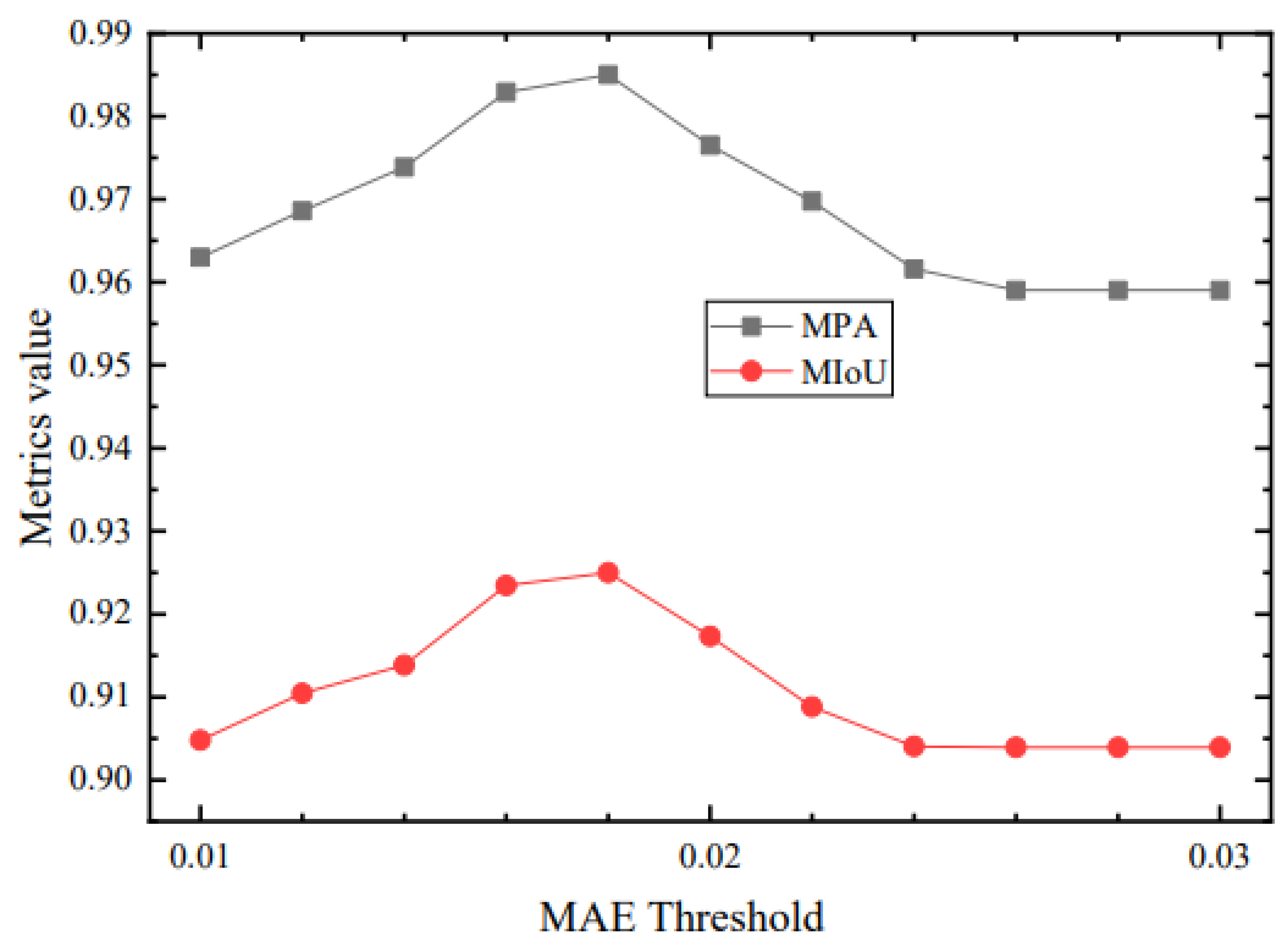
The testing phase employed 809 image sets. Three feature maps were generated via individual subnetworks. Subsequently, optimal segmentation was determined by assessing the mean absolute error (MAE) between and , compared to a pre-defined threshold . The intensity-depth unification (IDU) module retained features with (Figure 9, rows 1-2) and eliminated those with (rows 3-4). A range of eleven thresholds (0.01 to 0.03) was examined. Maximum performance, in terms of mean pixel accuracy (MPA) and mean intersection over union (MIoU), was achieved when , reaching 0.985 and 0.925, respectively.
Figure 9.
Segmentation output samples from the subnetworks and SIDNet.
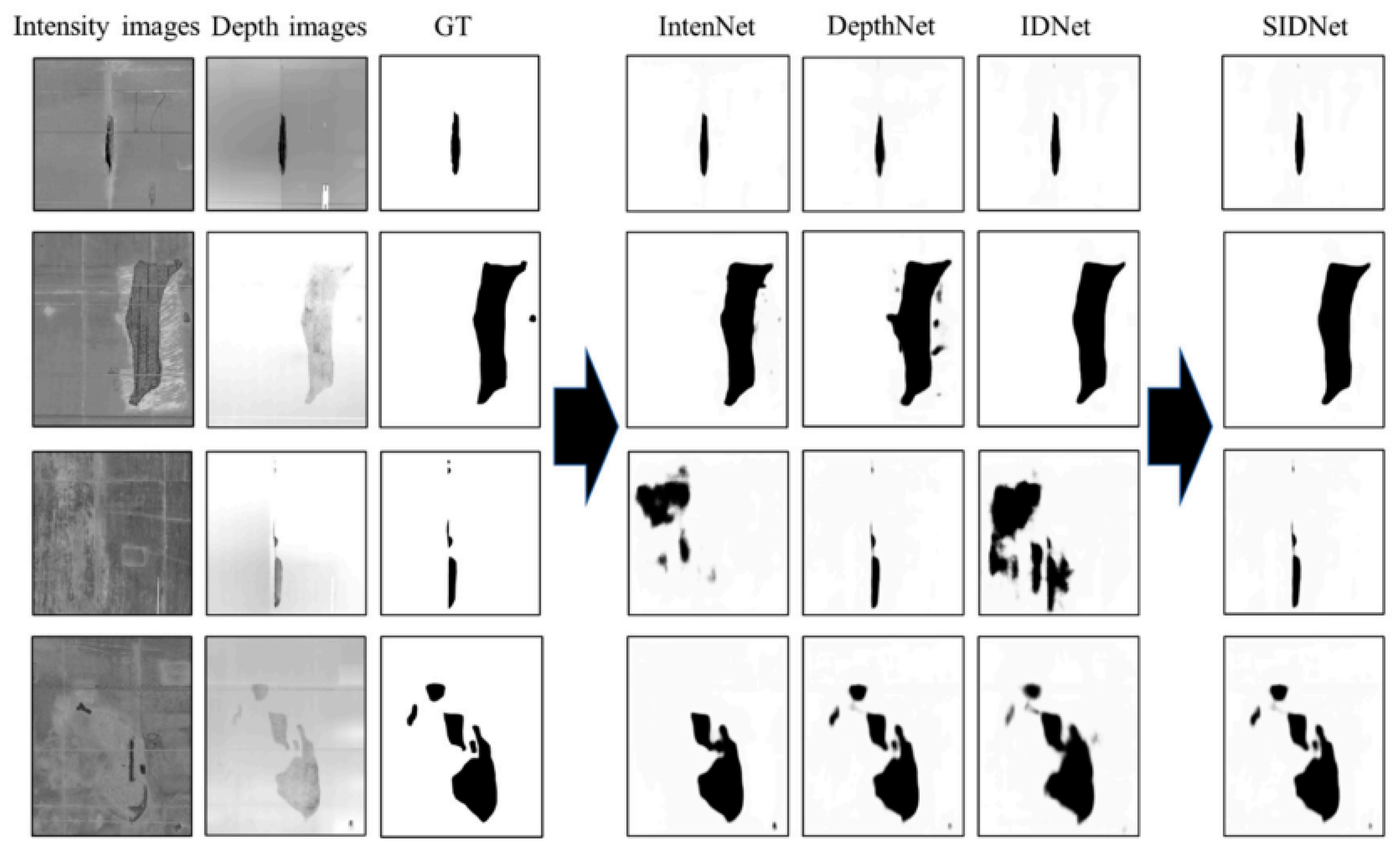
Figure 10.
Performance under varying MAE thresholds.
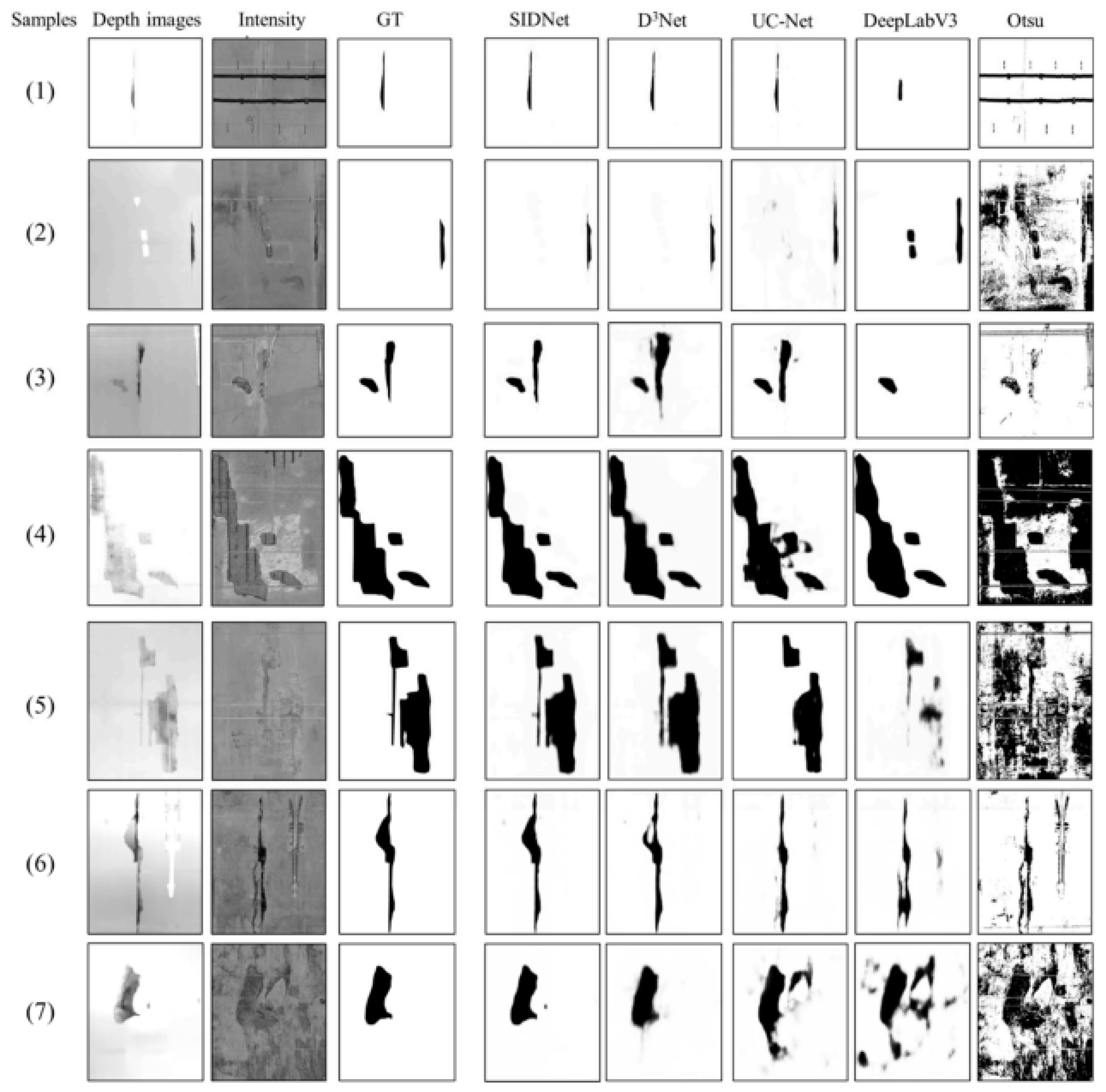
5.3. Comparative Evaluation of Segmentation Algorithms
To validate the utility of the IDU module, individual subnetwork outcomes (IntenNet, IDNet, and DepthNet) were compared with SIDNet and D3Net. Table 2 presents the MPA and MIoU metrics. SIDNet surpassed all models, highlighting the superior selectivity of the IDU mechanism in excluding suboptimal intensity data and favoring high-fidelity predictions from depth or intensity domains. The IDNet model outperformed DepthNet slightly, and both exceeded IntenNet’s performance. D3Net, employing depth-dependent unification (DDU), surpassed IntenNet but fell short of IDNet and DepthNet, underlining the importance of depth fidelity in spalling segmentation tasks.
Figure 11.
Visual comparison of detection outputs from diverse models.
5.4. Spalling Quantification Analysis
The area and volume of detected defects were estimated by aggregating spalling-associated pixels and corresponding depth values. Six examples are displayed in Figure 12, showing image inputs and their spatially mapped damage zones with color gradients.
The correlation between predicted and reference areas is illustrated in Figure 13. The regression slope and coefficient of determination () were 1.025 and 0.998, respectively. A weaker correlation () was observed between area and estimated volume, possibly due to inaccuracies in depth sensing or shallow spalling profiles.
5.5. Robustness Assessment of the Method
To assess method stability, point cloud datasets from forward and backward passes along a 500-meter tunnel were analyzed, comprising 21 defect instances. The root mean square error (RMSE) between the depth values was computed using:
where n is the number of pixels in defect regions, and denotes the depth deviation. An RMSE of 0.9 mm was obtained, aligning closely with the scanner’s nominal precision of 0.5 mm at 10 meters, indicating high internal consistency and system reliability.
6. 3D Visualization and Inspection Report
6.1. Methodology for Tunnel 3D Model Reconstruction
For effective spatial representation of tunnel lining degradation, it is essential to transform the classified 2D defect imagery into a three-dimensional context. This facilitates enhanced assessment of surface peeling phenomena in tunnel interiors. A viable strategy entails constructing a three-dimensional depiction of the tunnel by leveraging the acquired imagery and integrating it with the topological structure from the original point cloud dataset.
Figure 14 illustrates the overall process for generating a three-dimensional tunnel reconstruction. From the predicted outputs of the SIDNet framework, a 2D grid-based point cloud is synthesized by placing points at the centers of the corresponding defective pixels (Figure 14a–c). To elevate the 2D planar point data into a full 3D surface, a diagonal triangular meshing algorithm is employed. This algorithm connects each point with its three proximate neighbors to establish a triangular mesh surface (Figure 14d). Through systematic batch operations, this planar representation is morphed into a surface mesh of identical dimensions to the source images.
To project the 2D mesh into a volumetric domain, the planar data, including those associated with occluding elements, are mapped onto the spatial geometry of an elliptical tunnel structure (Figure 14e). This hypothetical model shares the same geometric parameters as the fitted ellipse described earlier. Defect images derived from the SIDNet outputs are subsequently overlaid onto the spatial mesh in accordance with the established correspondence between 2D coordinates and 3D surface vertices. The outcome is a colored 3D tunnel visualization embedding both positional and colorimetric data (Figure 14f).
6.2. Inspection Outcomes from a Tunnel Test Section
A tunnel segment of 75 meters in length was analyzed to demonstrate the robustness of the reconstruction framework. Point cloud data from 5-meter segments were processed into grayscale and depth map representations. These were then passed through the SIDNet network, producing segmented images of equal size. After segmentation, the small-scale images were concatenated to form a larger composite, which enhanced continuity and minimized frame count.
Figure 15a presents the stitched input image over a 75-meter span, with a width of 23.5 meters. Figure 15b displays the corresponding segmentation output generated from the SIDNet model, where spalling depth is depicted via a colormap gradient ranging from blue (0 m) to red (0.5 m).
A spatially immersive 3D model of the tunnel portion was produced using the segmented output, providing diverse visual perspectives of the tunnel interior (Figure 16). Depth metrics allowed the visualization of defect depth through varied chromatic cues. Additionally, obstructing objects could be filtered out in the rendered model. A detailed inspection report was generated (Table 3) cataloging each spalling defect’s position, angular extent, affected area, and volumetric displacement.
7. Discussion
7.1. Strengths of the Presented Framework
Precise determination of the material requirements for repairing tunnel deterioration necessitates exact evaluation of defect area and volume. Manual surveys often yield imprecise estimations due to reliance on visual approximation or single-point depth readings, which compromises volume accuracy.
Contemporary photogrammetry, recognized for its non-invasive nature, has gained traction in tunnel health diagnostics. High-resolution CCD systems mounted on movable platforms allow sequential capture of tunnel interiors. Although efficient in segmenting surface anomalies like fissures, leakage, and exfoliation, photogrammetry lacks sufficient depth perception to compute volumetric metrics.
The integrated methodology proposed herein enables accurate volumetric assessments by capturing detailed 3D coordinate data. Merging intensity and depth channels enhances segmentation fidelity in convolutional architectures. Tunnel lining geometry, obtained from Mobile Laser Scanning (MLS), facilitates high-density point collection even in constrained areas, enabling summation-based volume estimation of deteriorated regions. Furthermore, automatic report generation and visual reconstruction streamline inspection procedures and enhance digital documentation workflows.
7.2. Potential Implementation Scenarios
This framework is currently optimized for tunnel types conforming to circular or elliptical profiles—commonly found in railway and subway infrastructures. Future development should accommodate variable geometries typical in road tunnels. For metro systems with narrower diameters, denser depth sampling is feasible, enhancing spatial accuracy. Reduced interior surface area permits more granular data collection over defect zones.
The additional depth information positively contributes to inspection precision. The system is theoretically extendable to recognize other structural components, such as joint misalignments and bolt cavities, through inconsistencies in depth profiles. Utilizing 3D features substantially mitigates the misidentification caused by similarly colored objects, refining tunnel inspection methodologies.
8. Conclusion
A novel unified framework is introduced for the autonomous delineation and measurement of spalling defects within tunnel lining structures using point cloud data. A dedicated dataset, RTSD, was curated with over 8000 paired RGB and depth images. A multi-input DCNN model, SIDNet, was designed to extract features across both visual and depth modalities, significantly boosting segmentation reliability.
The resultant segmented images allow derivation of both spatial coverage and volume metrics of the spalling defects. Incorporation of 3D reconstruction further aids in spatial interpretation. The produced 3D surface mesh delivers a human-centric perspective, facilitating intuitive understanding of defect distribution. Automated reporting consolidates findings into a structured summary inclusive of spatial and volumetric insights.
Although point cloud granularity imposes resolution constraints, future refinements involving higher-resolution CCD systems and extended testing across diverse tunnel environments are expected to elevate performance.
References
- Liu, X.; Zhang, H. A review of tunnel defect detection methods using visual inspection and AI. Automation in Construction 2022, 135, 104129. [Google Scholar]
- Zhang, Y.; Wang, Q. Automated tunnel lining defect detection using deep learning on UAV images. IEEE Transactions on Intelligent Transportation Systems 2021. [Google Scholar]
- Li, M.; Chen, Z. Photogrammetry-based inspection for infrastructure: State-of-the-art and future trends. Journal of Infrastructure Systems 2023. [Google Scholar]
- Wang, T.; Liu, R. Application of LiDAR-based point cloud data in tunnel inspection. Remote Sensing 2021, 13, 1823. [Google Scholar]
- Chen, J.; Xu, Y. A survey of computer vision-based structural inspection using deep learning. Computer-Aided Civil and Infrastructure Engineering 2020, 35, 713–736. [Google Scholar]
- He, Z.; Wu, J. Deep learning-based crack damage detection using convolutional neural networks. Automation in Construction 2020, 110, 103018. [Google Scholar]
- Xu, W.; Liang, Y. Tunnel defect detection based on YOLOv5 with depth information fusion. Sensors 2022, 22, 5252. [Google Scholar]
- Gao, X.; Li, Y. RGB-D based concrete damage detection using CNNs. IEEE Access 2021, 9, 125089–125099. [Google Scholar]
Figure 8.
Loss progression curves for the subnetworks: (a) IntenNet, (b) IDNet, and (c) DepthNet.
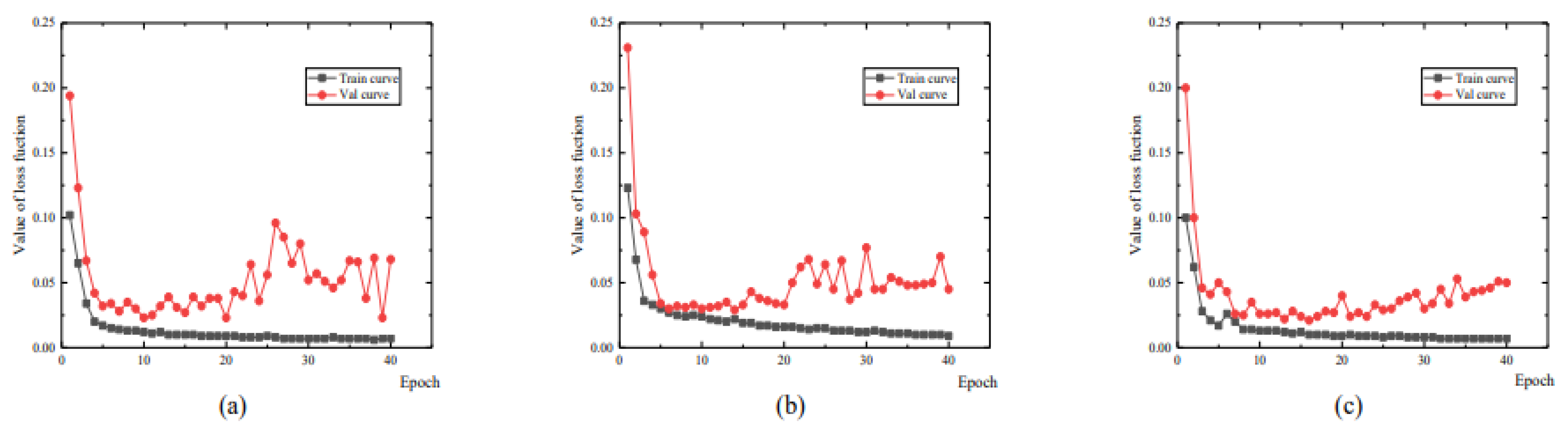
Figure 12.
Quantitative evaluation for six example samples.
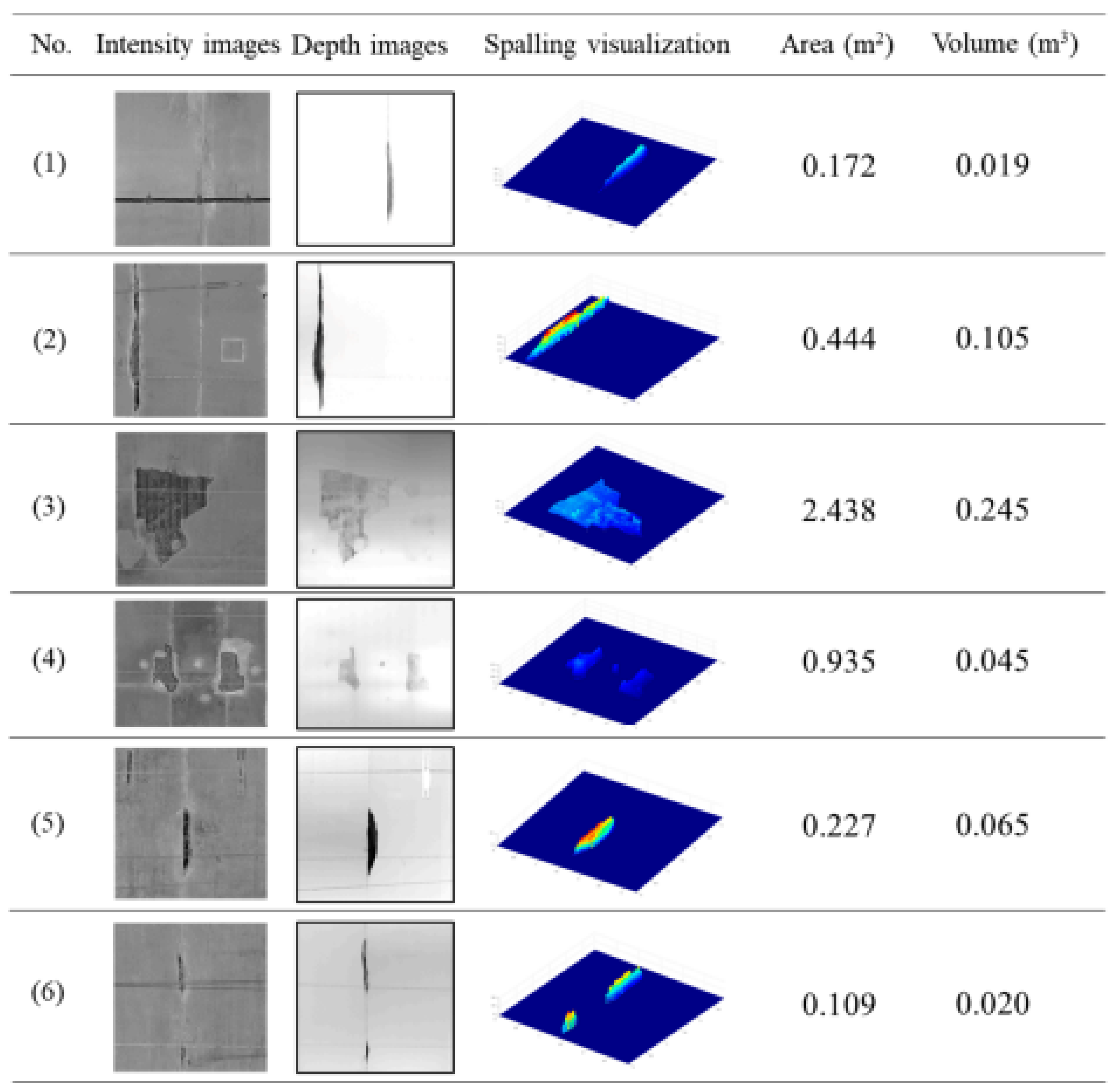
Figure 13.
Evaluation metrics: (a) predicted vs actual areas; (b) volume vs area correlation.
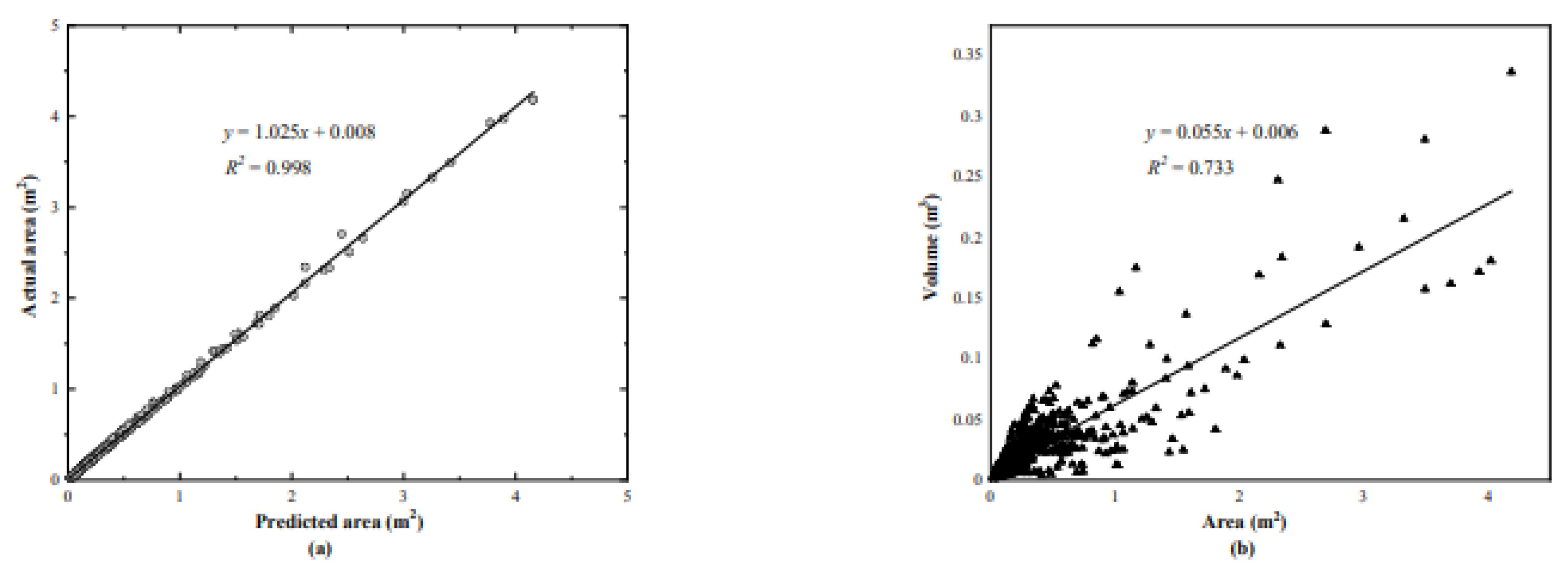
Figure 14.
Pipeline for constructing a three-dimensional tunnel model: (a) predicted defect image; (b) generation of 2D points; (c) creation of planar point cloud; (d) triangular mesh formation; (e) spatial surface projection; (f) overlay of segmented imagery on 3D mesh.
Figure 14.
Pipeline for constructing a three-dimensional tunnel model: (a) predicted defect image; (b) generation of 2D points; (c) creation of planar point cloud; (d) triangular mesh formation; (e) spatial surface projection; (f) overlay of segmented imagery on 3D mesh.
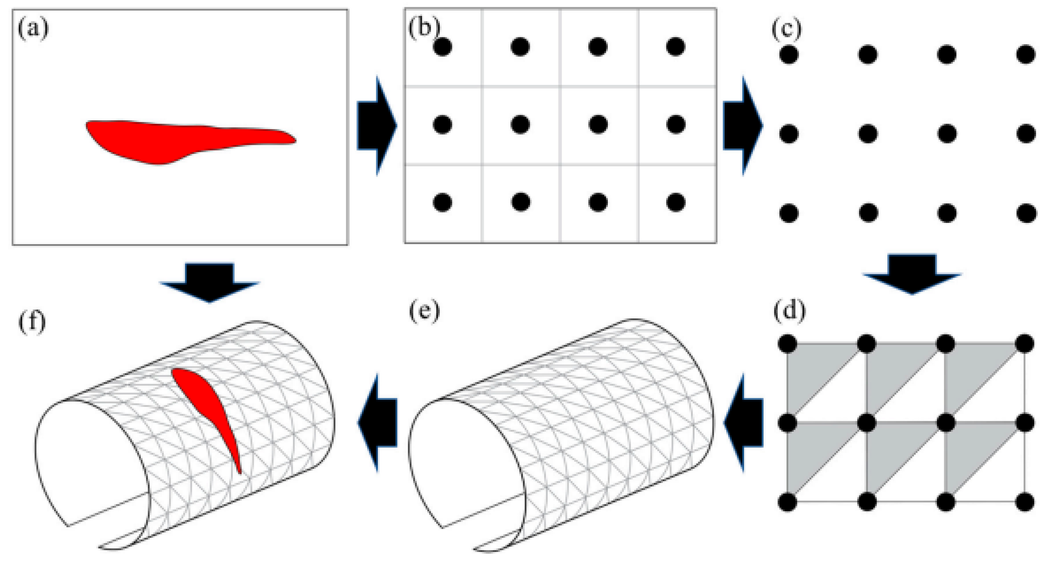
Figure 15.
Comparison for a 75-meter tunnel section: (a) composite intensity image; (b) segmented results with spalling defects magnified (depth: blue = 0 m to red = 0.5 m).
Figure 15.
Comparison for a 75-meter tunnel section: (a) composite intensity image; (b) segmented results with spalling defects magnified (depth: blue = 0 m to red = 0.5 m).
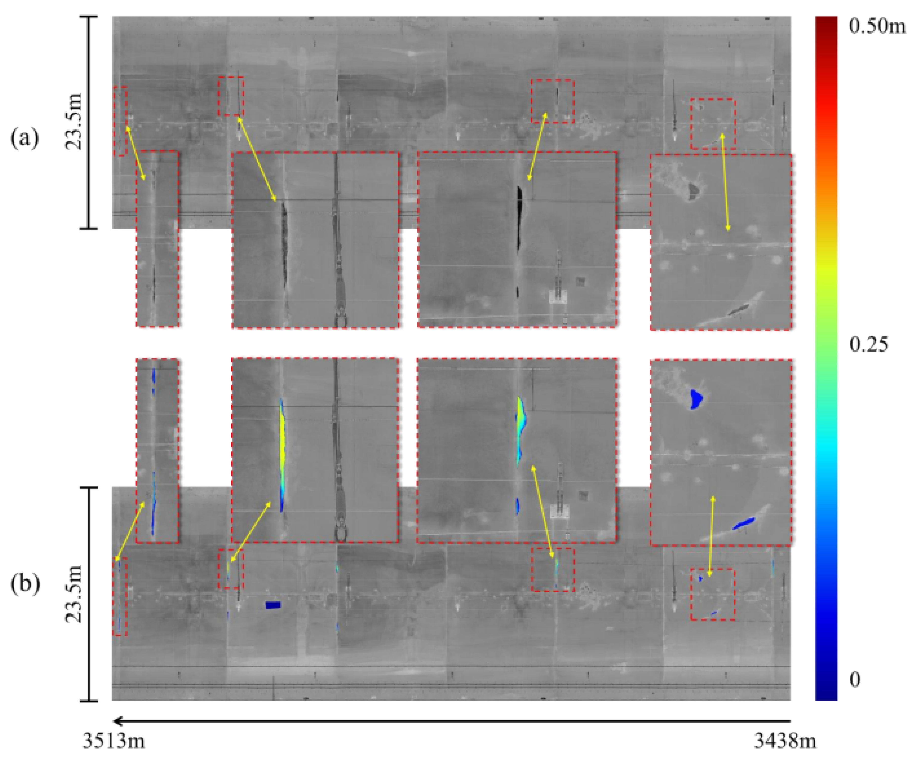
Figure 16.
3D defect visualization from multiple viewpoints: (a) entire tunnel segment; (b) longitudinal section; (c) and (d) front-facing views; specific defects circled in white.
Figure 16.
3D defect visualization from multiple viewpoints: (a) entire tunnel segment; (b) longitudinal section; (c) and (d) front-facing views; specific defects circled in white.
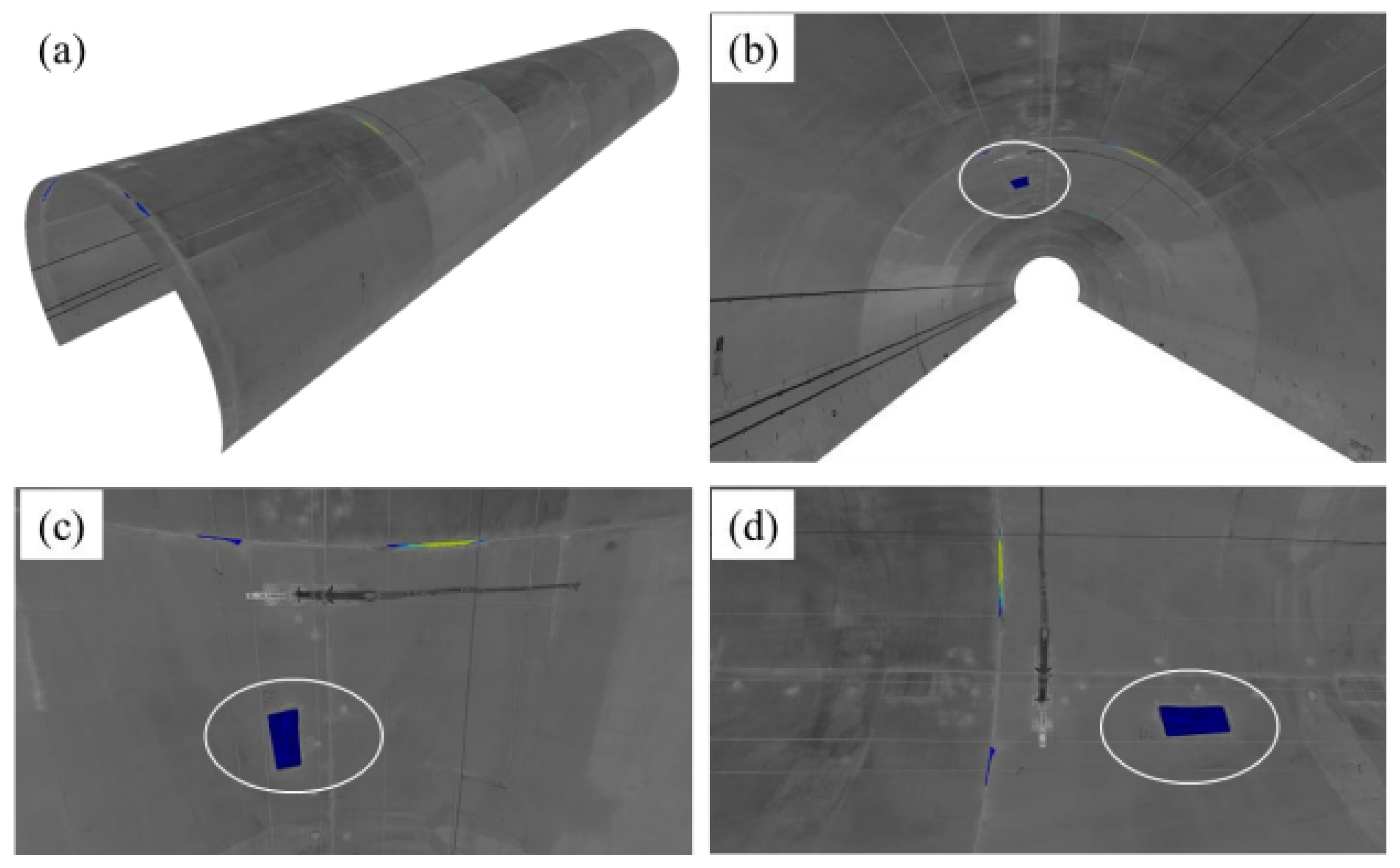

Table 1.
Distribution of Images in the RTSD Dataset
| Category | Training | Validation | Testing | Total |
|---|---|---|---|---|
| Intensity | 5664 | 1619 | 809 | 8092 |
| Depth | 5664 | 1619 | 809 | 8092 |
| GT | 5664 | 1619 | 809 | 8092 |
Table 2.
Performance Metrics Across Segmentation Approaches
| Model | MPA | MIoU |
|---|---|---|
| IntenNet | 0.904 | 0.838 |
| DepthNet | 0.957 | 0.905 |
| IDNet | 0.970 | 0.911 |
| SIDNet | 0.985 | 0.925 |
| D3Net | 0.935 | 0.874 |
| UC-Net | 0.971 | 0.907 |
| DeepLabV3+ | 0.881 | 0.792 |
| Otsu | 0.519 | 0.409 |
Table 3.
Quantitative report of spalling defects in a 75-meter tunnel segment.
| ID | Mileage (m) | Start Angle (∘) | End Angle (∘) | Area (m2) | Volume (m3) |
|---|---|---|---|---|---|
| 1 | 3438 | 132 | 134 | 0.031 | 0.017 |
| 2 | 3438 | 101 | 120 | 0.187 | 0.028 |
| 3 | 3446 | 96 | 103 | 0.086 | 0.004 |
| 4 | 3445 | 79 | 82 | 0.103 | 0.004 |
| 5 | 3463 | 103 | 122 | 0.254 | 0.053 |
| 6 | 3463 | 92 | 94 | 0.037 | 0.003 |
| 7 | 3488 | 115 | 121 | 0.107 | 0.017 |
| 8 | 3488 | 64 | 73 | 0.089 | 0.012 |
| 9 | 3495 | 80 | 85 | 1.253 | 0.075 |
| 10 | 3501 | 100 | 121 | 0.356 | 0.068 |
| 11 | 3501 | 76 | 80 | 0.121 | 0.010 |
| 12 | 3513 | 117 | 119 | 0.118 | 0.009 |
| 13 | 3513 | 115 | 116 | 0.065 | 0.004 |
| 14 | 3513 | 63 | 85 | 0.347 | 0.031 |
Disclaimer/Publisher’s Note: The statements, opinions and data contained in all publications are solely those of the individual author(s) and contributor(s) and not of MDPI and/or the editor(s). MDPI and/or the editor(s) disclaim responsibility for any injury to people or property resulting from any ideas, methods, instructions or products referred to in the content. |
© 2025 by the authors. Licensee MDPI, Basel, Switzerland. This article is an open access article distributed under the terms and conditions of the Creative Commons Attribution (CC BY) license (http://creativecommons.org/licenses/by/4.0/).
Copyright: This open access article is published under a Creative Commons CC BY 4.0 license, which permit the free download, distribution, and reuse, provided that the author and preprint are cited in any reuse.


