Submitted:
12 November 2025
Posted:
13 November 2025
You are already at the latest version
Abstract
This study introduced a pre-training method for machine learning-based climate prediction models. The method leverages the advantage of climate events (some theoretical knowledge) to address their limitation (small sample size). It consists of the following steps: generating artificial samples via composite analysis of high and low anomaly events, pre-training predictive models with these samples, and selecting an optimal pre-trained model that most closely matches the observational training set from numerous repeated experiments with only the model’s random number seeds being varied. Sensitivity experiments demonstrate that this pre-training method not only substantially improves predictive skills but also significantly reduces prediction instability. This simple and practical pre-training method is applicable not only to the climate prediction events in this study but also to all climate events for which composite analysis is applicable.
Keywords:
pre-training method
; artificial samples
; small sample size
1. Introduction
Statistical methods are essential tools for climate prediction, especially for longer lead times, during which the predictive skill of climate models tends to be considerably low [1,2,3,4,5,6,7,8,9,10]. Compared with traditional linear statistical methods (e.g., multivariate linear regression), machine learning methods that can capture complex nonlinear relationships are increasingly used in climate prediction studies [11,12,13,14,15,16,17,18,19,20,21,22,23,24,25,26]. Indeed, some machine learning-based climate prediction models have already been applied to practical operations, and the development and utilization of machine learning methods have emerged as an inevitable trend [27,28,29,30,31,32,33].
The volume of sample data required by machine learning-based statistical models is significantly larger than that demanded by linear statistical models, owing to the large number of tunable parameters. In the context of most climate research, the observation period is typically too short (less than 100 years) to yield an adequate quantity of samples used for model training. For this reason, simple machine learning models (i.e., those with only dozens of parameters) are preferred in some studies [34,35,36,37,38]. In other studies using relatively complex machine learning models (i.e., those with parameters far exceeding 1,000), numerical simulation results from different climate models are often utilized to expand the training sample size. Specifically, this approach requires climate models to have a certain level of reasonable predictive skill for such climate events, such as the ENSO index over the next 18 months [39,40], as well as upcoming monthly mean temperature [41] and seasonal precipitation [42]. In other machine learning application fields (e.g., image recognition and medical detection), a variety of mature techniques have been developed to tackle the small sample size issue [43,44,45,46,47,48]. However, the field of climate prediction has to date rarely seen research that explores technical methods for addressing small sample size challenges.
This study aims to develop a simple and applicable method for addressing small sample size challenges by integrating climate knowledge into existing techniques from other application fields. Notably, data augmentation and transfer learning are two primary approaches to tackling such issues in machine learning [49,50,51,52,53]. In climate prediction, composite analysis of abnormal events is a widely used method for mechanistic studies [54,55,56,57,58]. A single composite map can serve as an artificial composite sample to characterize the main features of such events [59,60,61,62]. In this study, data augmentation is first performed using these composite maps. The climate prediction model is then pre-trained on these augmented artificial samples, following the transfer learning framework. Finally, two approaches to utilizing the pre-trained models and their enhancement effects on the final predictive model are explored.
This study focuses on a climate prediction case: predicting July precipitation in the middle and lower reaches of the Yangtze River using prophase winter sea surface temperatures (SST). To enhance efficiency, a simple shallow neural network (NN) with two hidden layers is used to build the predictive model. The structure of this paper is organized as follows: Section 2 introduces the training process of the NN model and the corresponding sample data; Section 3 presents the effects of pre-training methods; Section 4 discusses the experience in using this pre-training method; and Section 5 provides the conclusions.
2. Data and Methods
2.1. The NN Predictive Model
This study focuses on demonstrating the pre-training method and its effects, while other aspects of the NN model are directly set and not discussed. Specifically, the input layer and two hidden layers contain 6, 8, and 3 neurons respectively. At the initial moment, all biases are set to zero, and the weights are random values following a normal distribution controlled by one random number seed (hereafter referred to as initialization seed). For model training, we adopt the early stopping method. This method is widely used to address the small sample sizes challenges, as it eliminates the need for an independent validation set [63,64,65]. The dropout technique is not used. The initial learning rate is set to 0.01, and it will be adaptively adjusted based on the gradient during the model training process [66].
2.2. Observed Samples and Composite Samples
The original station-observed monthly precipitation data are provided by the National Climate Center of the China Meteorological Administration. Based on this data, we first average the July precipitation amounts from all stations within the region into a single value. Next, we remove the decadal trend, calculate precipitation anomaly percentages, and finally moderately modify the abnormal precipitation while confining its range to -1 to 1. For brevity, this indexed precipitation will hereafter be denoted as Rain. The original monthly SST data were downloaded from the IRI/LDEO Climate Data Library [67]. Consistent with the processing of Rain, their decadal trend has also been removed. Here, 30 potential SST predictors are first extracted via Empirical Orthogonal Function (EOF) analysis on gridded SST data over the Pacific and Indian oceans, which provide predominant indicative signals [6][70]. Finally, only six EOF modes with the strongest correlation with Rain are selected. From 1951 to 2021, there are a total of 71 observed samples (one per year), with each sample containing one Rain index and six SST predictors (upper panel of Figure 1)
Inspired by the concept of data enhancement [71,72], we artificially generated additional samples based on composite analysis (hereafter referred to as composite samples). Among the 71 observed samples, 15 are high-Rain samples and 20 are low-Rain samples. Their composite maps are presented in the middle panel of Figure 1. In general, the high- and low-Rain composite maps share a consistent SST spatial distribution but exhibit opposing anomaly features. Correspondingly, their Rain index values are 0.771 and-0.646, respectively, and these two values are roughly opposites in magnitude. Previous studies have proposed many physical mechanisms to explain these composite maps [68,73,74,75]. Based on these mechanistic analyses, it is reasonable to infer that the enhancement of the prophase SST signal leads to increased rainfall. Therefore, some composite samples used for model training were artificially produced by scaling the composite maps (six SST predictors and corresponding Rain index). Here, both the high- and low-Rain composite maps were used to generate 20 composite samples each (40 in total), as shown in the lower panel of Figure 1. In the high- and low-Rain composite samples, the signal of the SST predictor increases linearly throughout, but the Rain growth rate slows down after reaching a certain level and ceases to increase when its absolute value exceeds 0.8. This nonlinear response of Rain to SST is consistent with climate background knowledge to a certain extent; it avoids the adverse impact of excessive linearization of composite samples on the training of NN models.
2.3. Model Training Procedures and Evaluation Metrics
In the field of machine learning, Loss (the difference between model's predicted values and actual labels) is commonly used to evaluate model performance. Different from this Loss, climate prediction models are typically evaluated using the linear correlation coefficient between their predicted values and observed data (hereafter referred to as Cor), which pays more attention to the sign correspondence between the two sequences. In this study, both Loss and Cor are adopted as evaluation metrics. Due to small sample sizes, the performance of trained models is often unstable and sensitive to the initialization seed [7][80]. Therefore, we demonstrate a group of the trained predictive model through 10 or 30 repeated experiments, where only the random number seeds (e.g., initialization seed) are varied. Accordingly, the Loss and Cor scores are represented by the mean values of these 10 or 30 repetitions, as well as their corresponding standard deviations.
Here, the NN model is first pre-trained on composite samples to yield a pre-trained model that can capture the common characteristics of high- and low-Rain samples. At this step, the Loss threshold for early stopping is set to 0.02. Subsequently, the pre-trained model undergoes further tuning based on the training set derived from observed samples, with training ceasing once the Loss falls below 0.4. It is noteworthy that the performance of the finally trained predictive models is sensitive to their corresponding pre-trained models. To enhance the performance of the final predictive model, one optimal pre-trained model is selected from all repeated experiment members via the Cor score on the training set right after the pre-training step; all final predictive models undergo further tuning based on training set and this optimal pre-trained model.
To demonstrate the effect of the pre-training method, we conducted three categorys of experiments. The first category is Without Pre-trained Models: the predictive NN model is trained directly on the training set. The second category is Different Pre-trained Models (i.e., without selecting the optimal pre-trained model): in the repeated experiments at pre-training step, one initialization seed corresponds to one pre-trained model, which in turn corresponds to one finally trained predictive model. The third category is One Fixed Pre-trained Model: one optimal pre-trained model is selected from a large number of repeated experiments right after the pre-training step, and this fixed pre-trained model is used in all subsequent further tuning experiments. The difference between the second and third categorys of experiments demonstrates the significance of selecting such a fixed optimal pre-trained model.
3. Results and Analysis
3.1. Performance of Pre-Trained Models
At the pre-training step, there is no need to worry about the overfitting issue. Since these 40 composite samples almost exhibit linear variation characteristics, the NN model can approximate them after only a small number of training iterations. As shown in the upper panel of Figure 2, the Rain values calculated by the 30 pre-trained models are nearly identical to those of the composite samples, with an average Loss of 0.019. This low Loss is attributed to the pre-defined training termination threshold, which is set to 0.02. Notably, although the 30 pre-trained models yield almost identical Rain values, their internal parameters (i.e., weights and biases) differ significantly (not shown). This parameter discrepancy explains why the performance of these models varies substantially on the observed samples (see the lower panel of Figure 2). Quantitatively, the Cor scores of these pre-trained models on the observed samples range from a minimum of 0.091 to a maximum of 0.440. For subsequent training with the training set (e.g., the first 45 observed samples), only the optimal pre-trained model, selected from these 30 models based on its linear correlation with the training set (the one corresponding to the red line in Figure 2), is used for the third category of experiment (i.e., One Fixed Pre-trained Model) in the following subsection.
3.2. Performance of Predictive Models on Training and Test Sets
Figure 3 illustrates the performance of the predictive models corresponding to the three experimental categorys introduced earlier. The first 45 observed samples were employed as the training set for pre-trained model further tuning. Given that the Loss threshold for early stopping is set to 0.4, the Loss scores of these three experimental categorys on the training set (i.e., 0.397, 0.396, and 0.396) are closely clustered and marginally below 0.4. Furthermore, the use of pre-trained models (the second and third experimental categorys) does not yield improvements in the Cor score with respect to training set performance. Compared to experiments without the pre-training method (where the Cor score is 0.651±0.009), those with a fixed pre-trained model exhibit a slightly lower Cor score (0.649±0.007); however, this difference falls within the uncertainty range. In terms of stability, predicted Rain values from the 30 predictive models vary significantly in those experiments without pre-trained models and with different pre-trained models. In contrast, experiments with a fixed pre-trained model demonstrate superior stability. This indicates that differences in the initial states of NN models are a key contributor to the instability of the final trained models.
In Figure 3, the last 26 observed samples are used as the test set, and this paragraph analyzes the performance of the final trained models on this set. It is evident that the final predictive models derived from the second and third experimental categorys, which utilize pre-trained models, exhibit better performance on the test set, particularly in terms of the Cor score. The reason for this is that pre-trained models capture the common characteristics of both high- and low-Rain samples; these characteristics, which can be taken as theoretical understanding, are applicable to both the training set and the test set. On the other hand, the process of further tuning pre-trained models with the training set may also disrupt the common characteristics that the pre-trained models originally captured. The more training iterations there are, the more these common characteristics are lost. In the 30 experiments with different pre-trained models (i.e., the second experimental category), most training iterations fall within the range of 5 to 15. In the 30 experiments with one fixed optimal pre-trained models (i.e., the third experimental category), the training iterations are only 3, 4, or 5. This explains why the third category of experiment can better improve the performance of the final predictive model on the test set.
Multi-model ensemble is a common-used method to enhance the stability of predictive models [37,81,82]. Figure 4 shows the results from model ensemble experiments. Each ensemble experiment comprises 30 model members (i.e., the average value of the 30 members is reported), with 10 groups of such ensemble experiments included in each category of experiment. As expected, the results of these model ensemble experiments demonstrate excellent stability, as shown in Figure 4, where the outcomes of the 10 groups of ensemble experiments almost completely overlap. Compared with individual models (Figure 3), the model ensemble also shows significant performance improvements on both the training set and the test set (Figure 4). Taking the second category of experiment as an example, the Loss and Cor scores on the training set improved from 0.396 and 0.653 (Figure 3) to 0.371 and 0.735 (Figure 4), while those on the test set improved from 0.470 and 0.382 (Figure 3) to 0.449 and 0.422 (Figure 4). Notably, in the third category of experiment, the use of one fixed pre-trained model leads to a relatively low uncertainty in the individual model results (Figure 3). Consequently, the improvement contributed by the multi-model ensemble is relatively weak (Figure 4). However, the third category of experiment still performs the best on the test set. Here, according to the chronological order of the observed samples, ~2/3 of the earlier samples are divided into the training set, and the remaining ~1/3 are used as the test set. When the sample size is small, the split of the training and test sets can significantly impact model performance. That is to say, the model evaluation results presented herein depend on the current splitting method and thus lack robustness.
3.3. Evaluation of Model Predictive Skill via Cross-Validation Experiments
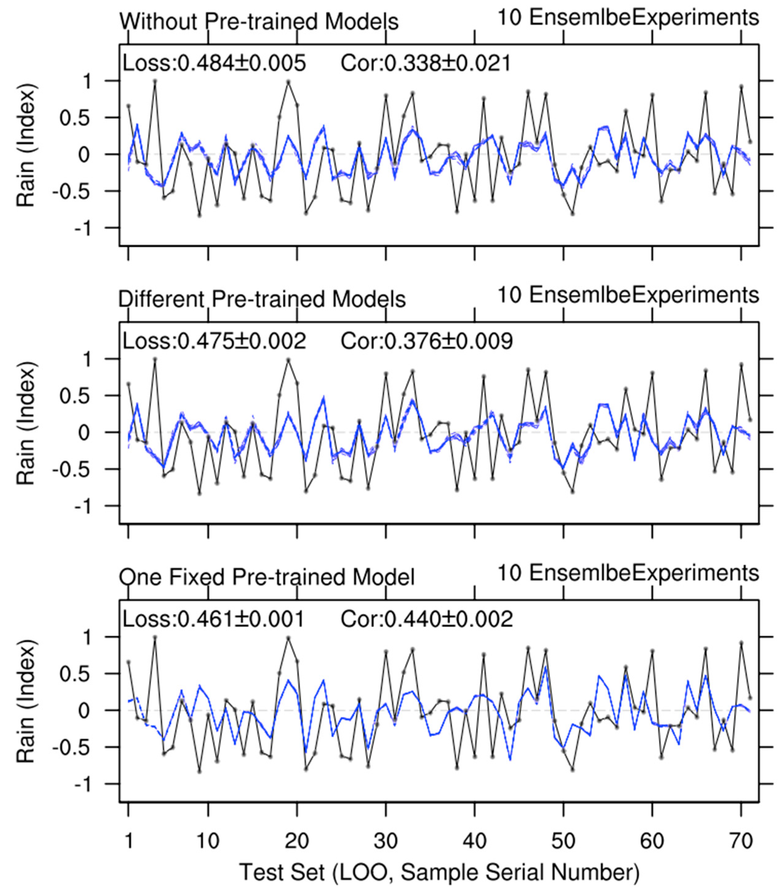
Cross-validation is a statistical method used to evaluate the performance and generalization ability of predictive models. Leave-One-Out (LOO), a special case of cross-validation, involves using one sample as the test set and the remaining samples as training data in each iteration [83–86]. To enhance the robustness of evaluating the predictive model’s performance, we conducted experiments using the LOO method (Figure 5). In the first category of experiments (i.e., without using the pre-training method), the Loss and Cor scores are 0.651 and 0.338, respectively. In the second category (i.e., using different pre-trained models), the predictive skill improved significantly, with Loss dropping to 0.475 and Cor rising to 0.376. In the third category (i.e., using one fixed optimal pre-trained model), the predictive skill improved even more, with Loss decreasing to 0.461 and Cor increasing to 0.440. Additionally, the stability of the model’s predictions has improved. In the first category of experiments, the standard deviations of Loss and Cor are 0.005 and 0.021, respectively. In the second category, their standard deviations dropped to 0.002 and 0.009, and in the third category, they decreased further to 0.001 and 0.002. In summary, the pre-training method not only improves the model’s predictive skills but also enhances the stability of its predictions, particularly when the “one fixed pre-trained model” approach is adopted.
4. Discussion
From a statistical perspective, composite maps for generating composite samples should be derived solely from abnormal events in the training set, not all observed samples. Notably, composite maps representing the common characteristics of both high and low anomaly events can be regarded as theoretical knowledge to a certain extent. This theoretical knowledge is not limited by samples and has extensibility. Correspondingly, composite maps from the training set are generally consistent with those from all observed samples. Thus, in this study’s experiments, the composite maps are fixed and not adjusted with changes in the training set. Additionally, the number of generated composite samples has little impact on the pre-training method’s performance, as these samples mainly follow linear scaling characteristics.
The pre-training method proposed herein is not only simpler but also more widely applicable as compared to that based on climate model simulation results. From the perspective of practical service needs, climate prediction focuses on abnormal events, which typically involve the excess or deficit of a specific climate variable (e.g., July precipitation). In most cases, composite analysis of high and low anomaly events reveals clear pre-event signals and influence mechanisms, with those for the two event types generally opposing each other. For climate events with such characteristics, the aforementioned method can be used to construct a pre-trained model that integrates climate theoretical knowledge. In contrast, climate models often fail to simulate abnormal events reasonably. Consequently, expanded samples derived from climate model simulations might have significant flaws and even be unfit for pre-training.
5. Conclusions
The main purpose of this study is to develop a simple and practical pre-training method for machine learning-based statistical models, taking advantage of the unique characteristics in climate research. This method adapts to the small sample size of climate events while enhancing the models’ predictive skills. Given the instability caused by small sample sizes, all figures present results from 10 or 30 repeated experiments (only the model’s random number seeds varied) to improve the robustness of model performance. Additionally, to eliminate the impact of training-test set division, the cross-validation method is adopted to further enhance the reliability of conclusions.
The pre-training method developed here involves two key steps: artificial sample generation and selection of the optimal pre-trained model. Artificial samples serve to incorporate the theoretical knowledge of climate events (i.e., generalizable common characteristics) into the pre-trained model. During subsequent tuning of the pre-trained model using the observational training set, some of these incorporated common characteristics will be lost. To mitigate such loss, the optimal pre-trained model that most closely matches the observational training set is selected from numerous repeated experiments. Experimental results demonstrate that pre-training with artificial samples significantly enhances the final predictive model’s performance on the test set. Additionally, selecting a fixed optimal pre-trained model not only further improves predictive performance but also substantially reduces prediction instability. In short, this pre-training method is a simple and practical approach to addressing the small sample size problems and enhancing predictive model performance.
Author Contributions
E.L. designed the study and provided overall support for this work. X.S. developed the neural network model Fortran code and conducted the experiments used in this study. X.S. and P.Z. analyzed the experimental results and drafted the manuscript. All authors have read and approved the final published version of the manuscript.
Funding
This research was funded by the National Natural Science Foundation of China (Grant 42475034) and the Qinghai Institute of Technology "Kunlun Elite" Research Project (Grant 2025-QLGKLYCZX-008). The APC was funded by the same funder.
Institutional Review Board Statement
Not applicable.
Informed Consent Statement
Not applicable.
Data Availability Statement
The Fortran code used in the experiments of this study (including the observed samples to be imported) and the plotting data of the experimental results (comprising plotting scripts and raw images) have been archived in a public repository: https://doi.org/10.5281/zenodo.17568411 (accessed on November 10, 2025).
Acknowledgments
This study was conducted in the High-Performance Computing Center of Nanjing University of Information Science & Technology. During the preparation of this manuscript, the authors used Doubao (online version, continuously updated) for the purposes of checking English writing grammar and moderately polishing the logical expression based on some revision suggestions. The authors have reviewed and edited the output and take full responsibility for the content of this publication.
Conflicts of Interest
The authors declare no conflicts of interest.
References
- Troccoli, A. Seasonal climate forecasting. Meteorol. Appl. 2010, 17, 251–268. [Google Scholar] [CrossRef]
- Li, W. Modern Climate Operations; China Meteorological Press: Beijing, China, 2012; pp. 170–201. ISBN 9787502954192. (In Chinese) [Google Scholar]
- Jia, X.; Chen, L.; Gao, H.; Wang, Y.; Ke, Z.; Liu, C.; Song, W.; Wu, T.; Feng, G.; Zhao, Z.; Li, W. Advances of the Short-range Climate Prediction in China. J. Appl. Meteorol. Sci. 2013, 24, 15. (In Chinese) [Google Scholar] [CrossRef]
- Wang, H.; Fan, K.; Sun, J.; Li, S.; Lin, Z.; Zhou, G.; Chen, L.; Lang, X.; Li, F.; Zhu, Y.; Chen, H.; Zheng, F. A review of seasonal climate prediction research in China. Adv. Atmos. Sci. 2015, 32, 149–168. [Google Scholar] [CrossRef]
- Wei, F. Progresses on Climatological Statistical Diagnosis and Prediction Methods———In Commemoration of the 50 Anniversaries of CAMS Establishment. J. Appl. Meteor. Sci. 2006, 17, 736–742. [Google Scholar] [CrossRef]
- Wang, X.; Song, L.; Wang, G.; Ren, H.; Wu, T.; Jia, X.; Wu, H.; Wu, J. Operational climate prediction in the era of big data in China: Reviews and prospects. J. Meteorol. Res. 2016, 30, 444–456. [Google Scholar] [CrossRef]
- Liu, Y.; Ren, H.; Zhang, P.; Zuo, J.; Tian, B.; Wan, J.; Li, Y. Application of the Hybrid Statistical Downscaling Model in Summer Precipitation Prediction in China. Clim. Environ. Res. 2020, 25, 163–171. (In Chinese) [Google Scholar] [CrossRef]
- Niu, D.; Diao, L.; Zang, Z.; Che, H.; Zhang, T.; Chen, X. A Machine-Learning Approach Combining Wavelet Packet Denoising with Catboost for Weather Forecasting. Atmosphere 2021, 12, 1618. [Google Scholar] [CrossRef]
- Yang, Z.; Tuo, Y.; Yang, J.; Wu, Y.; Gong, Z.; Feng, G. Integrated Prediction of Summer Precipitation in China Based on Multi Dynamic-Statistic Methods. Chin. J. Geophys. 2024, 67, 982–996. (In Chinese) [Google Scholar] [CrossRef]
- Bommer, P.L.; Kretschmer, M.; Spuler, F.R.; Bykov, K.; Höhne, M.M.-C. Deep Learning Meets Teleconnections: Improving S2S Predictions for European Winter Weather. Mach. Learn. Earth 2025, 1, 015002. [Google Scholar] [CrossRef]
- Deshpande, R.R. On the Rainfall Time Series Prediction Using Multilayer Perceptron Artificial Neural Network. Int. J. Emerg. Technol. Adv. Eng. 2012, 2, 2250–2459. [Google Scholar]
- Mekanik, F.; Imteaz, M.A.; Gato-Trinidad, S.; Elmahdi, A. Multiple Regression and Artificial Neural Network for Long-Term Rainfall Forecasting Using Large Scale Climate Modes. J. Hydrol. 2013, 503, 11–21. [Google Scholar] [CrossRef]
- Deo, R.C.; Sahin, M. Application of the Artificial Neural Network Model for Prediction of Monthly Standardized Precipitation and Evapotranspiration Index Using Hydrometeorological Parameters and Climate Indices in Eastern Australia. Atmos. Res. 2015, 161–162, 65–81. [Google Scholar] [CrossRef]
- Chi, J.; Kim, H.-c. Prediction of Arctic Sea Ice Concentration Using a Fully Data Driven Deep Neural Network. Remote Sens. 2017, 9, 1305. [Google Scholar] [CrossRef]
- Hartigan, J.; MacNamara, S.; Leslie, L.M. Application of Machine Learning to Attribution and Prediction of Seasonal Precipitation and Temperature Trends in Canberra, Australia. Climate 2020, 8, 76. [Google Scholar] [CrossRef]
- Geng, H.; Wang, T. Spatiotemporal Model Based on Deep Learning for ENSO Forecasts. Atmosphere 2021, 12, 810. [Google Scholar] [CrossRef]
- Ham, Y.-G.; Kim, J.-H.; Kim, E.-S.; On, K.-W. Unified Deep Learning Model for El Niño/Southern Oscillation Forecasts by Incorporating Seasonality in Climate Data. Sci. Bull. 2021, 66, 1358–1366. [Google Scholar] [CrossRef] [PubMed]
- Hussein, E.A.; Ghaziasgar, M.; Thron, C.; Vaccari, M.; Bagula, A. Basic Statistical Estimation Outperforms Machine Learning in Monthly Prediction of Seasonal Climatic Parameters. Atmosphere 2021, 12, 539. [Google Scholar] [CrossRef]
- Kim, H.; Ham, Y.G.; Joo, Y.S.; Son, S.W. Deep Learning for Bias Correction of MJO Prediction. Nat. Commun. 2021, 12, 3087. [Google Scholar] [CrossRef]
- El-Habil, B.Y.; Abu-Naser, S.S. Global Climate Prediction Using Deep Learning. J. Theor. Appl. Inf. Technol. 2022, 100, 4824–4838. [Google Scholar]
- Kishtawal, C.M.; Basu, S.; Patadia, F.; Thapliyal, P.K. Forecasting Summer Rainfall over India Using Genetic Algorithm. Geophys. Res. Lett. 2003, 30, 23. [Google Scholar] [CrossRef]
- Yao, Z.; Xu, D.; Wang, J.; Ren, J.; Yu, Z.; Yang, C.; Xu, M.; Wang, H.; Tan, X. Predicting and Understanding the Pacific Decadal Oscillation Using Machine Learning. Remote Sens. 2024, 16, 2261. [Google Scholar] [CrossRef]
- Wang, T.; Huang, P. Superiority of a Convolutional Neural Network Model over Dynamical Models in Predicting Central Pacific ENSO. Adv. Atmos. Sci. 2024, 41, 141–154. [Google Scholar] [CrossRef]
- Fernandez, M.A.; Barnes, E.A. Multi-Year-to-Decadal Temperature Prediction using a Machine Learning Model-Analog Framework. arXiv 2025, arXiv:2502.17583 physics.ao-ph, physics.ao–ph. [Google Scholar] [CrossRef]
- Patel, A.; Mark, B.G.; Haritashya, U.K.; Bawa, A. Twenty first century snow cover prediction using deep learning and climate model data in the Teesta basin, eastern Himalaya. Clim. Dyn. 2025, 63, 156. [Google Scholar] [CrossRef]
- You, J.; Liang, P.; Yang, L.; Zhang, T.; Xie, L.; Murtugudde, R. Mechanisms of Intraseasonal Oscillation in Equatorial Surface Currents in the Pacific Ocean Identified by Neural Network Models. J. Geophys. Res. Oceans 2025, 130, e2024JC021514. [Google Scholar] [CrossRef]
- Reichstein, M.; Camps-Valls, G.; Stevens, B.; Jung, M.; Denzler, J.; Carvalhais, N.; Prabhat. Deep learning and process understanding for data-driven Earth system science. Nature 2019, 566, 195–204. [Google Scholar] [CrossRef]
- Irrgang, C.; Boers, N.; Sonnewald, M.; Barnes, E.A.; Kadow, C.; Staneva, J.; Saynisch-Wagner, J. Towards neural Earth system modelling by integrating artificial intelligence in Earth system science. Nat. Mach. Intell. 2021, 3, 667–674. [Google Scholar] [CrossRef]
- Sun, J.; Cao, Z.; Li, H.; Qian, S.; Wang, X.; Yan, L.; Xue, W. Application of Artificial Intelligence Technology in Numerical Weather Prediction. J. Appl. Meteorol. Sci. 2021, 32, 1–11. (In Chinese) [Google Scholar] [CrossRef]
- Yang, S.; Ling, F.; Ying, W.; Yang, S.; Luo, J. A brief overview of the application of artificial intelligence to climate prediction. Trans. Atmos. Sci. 2022, 45, 641–659. (In Chinese) [Google Scholar] [CrossRef]
- Chen, L.; Han, B.; Wang, X.; Zhao, J.; Yang, W.; Yang, Z. Machine Learning Methods in Weather and Climate Applications: A Survey. Appl. Sci. 2023, 13, 12019. [Google Scholar] [CrossRef]
- Wang, G.-G.; Cheng, H.L.; Zhang, Y.M.; Yu, H. ENSO analysis and prediction using deep learning: A review. Neurocomput. 2023, 520, 216–229. [Google Scholar] [CrossRef]
- Sun, C.; Zhang, T.; Hu, J. A Review of the Application of Artificial Intelligence Methods in Meteorology. Desert Oasis Meteorol. 2025, 19, 60–67. (In Chinese) [Google Scholar] [CrossRef]
- Wu, A.; Hsieh, W.W.; Tang, B. Neural network forecasts of the tropical Pacific sea surface temperatures. Neural Netw. 2006, 19, 145–154. [Google Scholar] [CrossRef] [PubMed]
- Guo, J.; Guo, S.; Chen, H.; Yan, B.; Zhang, J.; Zhang, H. Prediction of Changes of Precipitation in Hanjiang River Basin Using Statistical Downscaling Method Based on ANN. Eng. J. Wuhan Univ. 2010, 43, 148–152. (In Chinese) [Google Scholar]
- Shen, H. Prediction of Summer Precipitation in China based on Machine Learning. Master's Thesis, Tsinghua University, Beijing, China, 2019. (In Chinese). [Google Scholar] [CrossRef]
- Anochi, J.A.; de Almeida, V.A.; de Campos Velho, H.F. Machine Learning for Climate Precipitation Prediction Modeling over South America. Remote Sens. 2021, 13, 2468. [Google Scholar] [CrossRef]
- Ham, Y.-G.; Kim, J.-H.; Luo, J.-J. Deep learning for multi-year ENSO forecasts. Nature 2019, 573, 568–572. [Google Scholar] [CrossRef] [PubMed]
- Sreeraj, P.; Balaji, B.; Paul, A.; Francis, P.A. A probabilistic forecast for multi-year ENSO using Bayesian convolutional neural network. Environ. Res. Lett. 2024, 19, 124023. [Google Scholar] [CrossRef]
- He, S.; Wang, H.; Li, H.; Zhao, J. Machine learning and its potential application to climate prediction. Trans. Atmos. Sci. 2021, 44, 26–38. (In Chinese) [Google Scholar] [CrossRef]
- Jin, W.; Luo, Y.; Wu, T.; Huang, X.; Xue, W.; Yu, C. Deep Learning for Seasonal Precipitation Prediction over China. J. Meteorol. Res. 2022, 36, 271–281. [Google Scholar] [CrossRef]
- Wang, Y.X.; Hebert, M. Learning to Learn: Model Regression Networks for Easy Small Sample Learning. In Computer Vision – ECCV 2016, Leibe, B., Matas, J., Sebe, N., Welling, M., Eds.; Springer: Cham, Switzerland, 2016; Volume 9910, pp. 616–634. ISBN 978-3-319-46466-4. [Google Scholar] [CrossRef]
- Kim, D.H.; MacKinnon, T. Artificial intelligence in fracture detection: transfer learning from deep convolutional neural networks. Clin. Radiol. 2018, 73, 439–445. [Google Scholar] [CrossRef] [PubMed]
- Keshari, R.; Ghosh, S.; Chhabra, S.; Vatsa, M.; Singh, R. Unravelling Small Sample Size Problems in the Deep Learning World. In Proceedings of the 2020 IEEE Sixth International Conference on Multimedia Big Data (BigMM), IEEE: New Delhi, India; 2020; pp. 134–143. [Google Scholar] [CrossRef]
- Soh, J.W.; Cho, S.; Cho, N.I. Meta-transfer learning for zero-shot super-resolution. In Proceedings of the IEEE/CVF Conference on Computer Vision and Pattern Recognition; IEEE: Seattle, WA, USA, 2009; pp. 3516–3525. [Google Scholar]
- Avuçlu, E. A new data augmentation method to use in machine learning algorithms using statistical measurements. Measurement 2021, 180, 109577. [Google Scholar] [CrossRef]
- Javaheri, T.; Homayounfar, M.; Amoozgar, Z.; Reiazi, R.; Homayounieh, F.; Abbas, E.; Laali, A.; Radmard, A.R.; Gharib, M.H.; Mousavi, S.A.J.; et al. CovidCTNet: An Open-Source Deep Learning Approach to Diagnose COVID-19 Using Small Cohort of CT Images. npj Digit. Med. 2021, 4, 29. [Google Scholar] [CrossRef]
- Yang, Q. Transfer Learning beyond Text Classification. In Advances in Machine Learning; Zhou, Z.H., Washio, T., Eds.; Springer: Berlin, Heidelberg, Germany, 2009; Volume 5828, pp. 25–43. ISBN 978-3-642-05224-8. [Google Scholar] [CrossRef]
- Yang, J.; Yu, X.; Xie, Z.-Q.; Zhang, J.-P. A novel virtual sample generation method based on Gaussian distribution. Knowl.-Based Syst. 2011, 24, 740–748. [Google Scholar] [CrossRef]
- Hoyle, B.; Rau, M.M.; Bonnett, C.; Seitz, S.; Weller, J. Data augmentation for machine learning redshifts applied to Sloan Digital Sky Survey galaxies. Mon. Not. R. Astron. Soc. 2015, 450, 305–316. [Google Scholar] [CrossRef]
- Chepurko, N.; Marcus, R.; Zgraggen, E.; Fernandez, R.C.; Kraska, T.; Karger, D. ARDA: Automatic Relational Data Augmentation for Machine Learning. arXiv 2020, arXiv:2003.09758. [Google Scholar] [CrossRef]
- Tao, Q.; Yu, J.; Mu, X.; Jia, X.; Shi, R.; Yao, Z.; Wang, C.; Zhang, H.; Liu, X. Machine learning strategies for small sample size in materials science. Sci. China Mater. 2025, 68, 387–405. [Google Scholar] [CrossRef]
- Yoden, S.; Yamaga, T.; Pawson, S.; Langematz, U. A composite analysis of the stratospheric sudden warmings simulated in a perpetual January integration of the Berlin TSM GCM. J. Meteorol. Soc. Japan. Ser. II 1999, 77, 431–445. [Google Scholar] [CrossRef]
- Hao, L.; Min, J. Why precipitation has reduced in North China. In Proceedings of the 2011 International Conference on Remote Sensing, Environment and Transportation Engineering, IEEE: Nanjing, China, 2011; pp. 940–943. 940. [CrossRef]
- Wang, N.; Fang, J.; Cui, W.; Xiao, L.; Wang, Q. Main Circulation Characteristics of Summer Droughts and Floods in Shaanxi. J. Arid Meteorol. 2013, 31, 702–707. [Google Scholar] [CrossRef]
- Li, Y.; Zhu, Y.; Wang, Y. Inlfuencing Large-scale Circulation Factor Analysis of Summer Temperature in Heilongjiang Province. Adv. Meteor. Sci. Technol. 2015, 5, 48–52. (In Chinese) [Google Scholar] [CrossRef]
- Welhouse, L.J.; Lazzara, M.A.; Keller, L.M.; Tripoli, G.J.; Hitchman, M.H. Composite Analysis of the Effects of ENSO Events on Antarctica. J. Climate 2016, 29, 1797–1808. [Google Scholar] [CrossRef]
- Hoel, P.G. Introduction to Mathematical Statistics, 4th ed.; John Wiley & Sons, Inc.: New York, London, 1971; pp. 1–409. ISBN 9780471403654. [Google Scholar] [CrossRef]
- Wei, F. Modern Climate Statistical Diagnosis and Prediction Technology, 2nd ed.; China Meteorological Press: Beijing, China, 2007; ISBN 9787502942991. (In Chinese) [Google Scholar]
- Wilks, D.S. Statistical Methods in the Atmospheric Sciences; China Meteorological Press: Beijing, China, 2017; ISBN 9787502964016. (In Chinese) [Google Scholar]
- Mudelsee, M. Statistical Analysis of Climate Extremes; Cambridge University Press: Cambridge, UK, 2020; ISBN 9781108791465. [Google Scholar]
- Nguyen, M.H.; Abbass, H.A.; McKay, R.I. Stopping criteria for ensemble of evolutionary artificial neural networks. Appl. Soft Comput. 2005, 6, 100–107. [Google Scholar] [CrossRef]
- Mahsereci, M.; Balles, L.; Lassner, C.; Hennig, P. Early Stopping without a Validation Set. arXiv 2017, arXiv:1703.09580. [Google Scholar] [CrossRef]
- Dodge, J.; Ilharco, G.; Schwartz, R.; Farhadi, A.; Hajishirzi, H.; Smith, N. Fine-Tuning Pretrained Language Models: Weight Initializations, Data Orders, and Early Stopping. arXiv 2020, arXiv:2002.06305. [Google Scholar] [CrossRef]
- Kingma, D.P.; Ba, J. Adam: A Method for Stochastic Optimization. CoRR 2014, abs/1412.6980. https://api.semanticscholar.org/CorpusID:6628106.
- Kaplan, A.; Cane, M.A.; Kushnir, Y.; Clement, A.C.; Blumenthal, M.B.; Rajagopalan, B. Analyses of global sea surface temperature 1856–1991. J. Geophys. Res. 1998, 103, 18567–18589. [Google Scholar] [CrossRef]
- Chan, J.C.L.; Zhou, W. PDO, ENSO and the early summer monsoon rainfall over south China. Geophys. Res. Lett. 2005, 32, L08810. [Google Scholar] [CrossRef]
- Fan, K.; Wang, H.; Choi, Y.-J. A Physical Statistical Prediction Model for Summer Precipitation in the Middle and Lower Reaches of the Yangtze River. Chin. Sci. Bull. 2007, 52, 2900–2905. (In Chinese) [Google Scholar]
- Liu, B.; Zhu, C. Potential Skill Map of Predictors Applied to the Seasonal Forecast of Summer Rainfall in China. J. Appl. Meteor. Sci. 2020, 31, 570–582. [Google Scholar] [CrossRef]
- Taylor, L.; Nitschke, G. Improving Deep Learning with Generic Data Augmentation. In Proceedings of the 2018 IEEE Symposium Series on Computational Intelligence (SSCI), Bangalore, India, 2018; pp. 1542–1547. [CrossRef]
- Iglesias, G.; Talavera, E.; González-Prieto, Á.; Mozo, A.; Gómez-Canaval, S. Data Augmentation Techniques in Time Series Domain: A Survey and Taxonomy. Neural Comput. Appl. 2023, 35, 10123–10145. [Google Scholar] [CrossRef]
- Jiang, T.; Zhang, Q.; Zhu, D.; Wu, Y. Yangtze Floods and Droughts (China) and Teleconnections with ENSO Activities (1470–2003). Quat. Int. 2006, 144, 29–37. [Google Scholar] [CrossRef]
- Zhang, R.H.; Min, Q.Y.; Su, J.Z. Impact of El Niño on Atmospheric Circulations over East Asia and Rainfall in China: Role of the Anomalous Western North Pacific Anticyclone. Sci. China Earth Sci. 2017, 60, 1124–1132. [Google Scholar] [CrossRef]
- Xu, B.; Li, G.; Gao, C.; Yan, H.; Wang, Z.; Li, Y.; Zhu, S. Asymmetric Effect of El Niño—Southern Oscillation on the Spring Precipitation over South China. Atmosphere 2021, 12, 391. [Google Scholar] [CrossRef]
- Luo, Q.; Deng, F.-Q.; Bao, J.-D. Stabilization of a Generalized Stochastic Neural Network with Distributed Parameters. In Proceedings of the 2003 International Conference on Machine Learning and Cybernetics (ICMLC), Xi'an, China; 2003; Volume 2, pp. 1231–1236. [Google Scholar] [CrossRef]
- Elisseeff, A.; Evgeniou, T.; Pontil, M. Stability of Randomized Learning Algorithms. J. Mach. Learn. Res. 2005, 6, 55–79. [Google Scholar]
- Luo, K.; Jia, Z.; Gao, W. Strong and Weak Stability of Randomized Learning Algorithms. In Proceedings of the 2012 IEEE 14th International Conference on Communication Technology (ICCT), Chengdu, China; 2012; pp. 887–891. [Google Scholar] [CrossRef]
- Talukder, S.; Kumar, R. Robust Stability of Neural-Network-Controlled Nonlinear Systems With Parametric Variability. IEEE Trans. Syst., Man, Cybern. Syst. 2023, 53, 4820–4832. [Google Scholar] [CrossRef]
- Gan, L.Q.; Zikry, T.M.; Allen, G.I. Are Machine Learning Interpretations Reliable? A Stability Study on Global Interpretations. arXiv 2025, arXiv:2505.15728. [Google Scholar] [CrossRef]
- Christiansen, B. Analysis of Ensemble Mean Forecasts: The Blessings of High Dimensionality. Mon. Wea. Rev. 2019, 147, 1699–1712. [Google Scholar] [CrossRef]
- Snieder, E.; Abogadil, K.; Khan, U.T. Resampling and Ensemble Techniques for Improving ANN-Based High-Flow Forecast Accuracy. Hydrol. Earth Syst. Sci. 2021, 25, 2543–2566. [Google Scholar] [CrossRef]
- Cawley, G.C. Leave-One-Out Cross-Validation Based Model Selection Criteria for Weighted LS-SVMs. In Proceedings of The 2006 IEEE International Joint Conference on Neural Network, Vancouver, BC, Canada, 2006; pp. 1661–1668. [CrossRef]
- Wu, J.; Mei, J.; Wen, S.; Liao, S.; Chen, J.; Shen, Y. A Self-Adaptive Genetic Algorithm-Artificial Neural Network Algorithm with Leave-One-Out Cross Validation for Descriptor Selection in QSAR Study. J. Comput. Chem. 2010, 31, 1956–1968. [Google Scholar] [CrossRef]
- Volpe, V.; Manzoni, S.; Marani, M. Leave-One-Out Cross-Validation. In Encyclopedia of Machine Learning; Sammut, C., Webb, G.I., Eds.; Springer: Boston, MA, USA, 2011; pp. 24–45. ISBN 978-0-387-30768-8. [Google Scholar] [CrossRef]
- Opper, M.; Winther, O. Gaussian Processes and SVM: Mean Field Results and Leave-One-Out. In Advances in Large Margin Classifiers; Smola, A.J., Bartlett, P., Schölkopf, B., Schuurmans, D., Eds.; MIT Press: Cambridge, MA, USA, 2000; ISBN 0262194481. [Google Scholar]
Figure 1.
Observed samples (upper panel), composite maps (middle panel) of 15 high-Rain samples (left) and 20 low-Rain samples (right), and composite samples (lower panel). Each sample contains one Rain index (in black) and six EOF modes of SST (in color).
Figure 1.
Observed samples (upper panel), composite maps (middle panel) of 15 high-Rain samples (left) and 20 low-Rain samples (right), and composite samples (lower panel). Each sample contains one Rain index (in black) and six EOF modes of SST (in color).
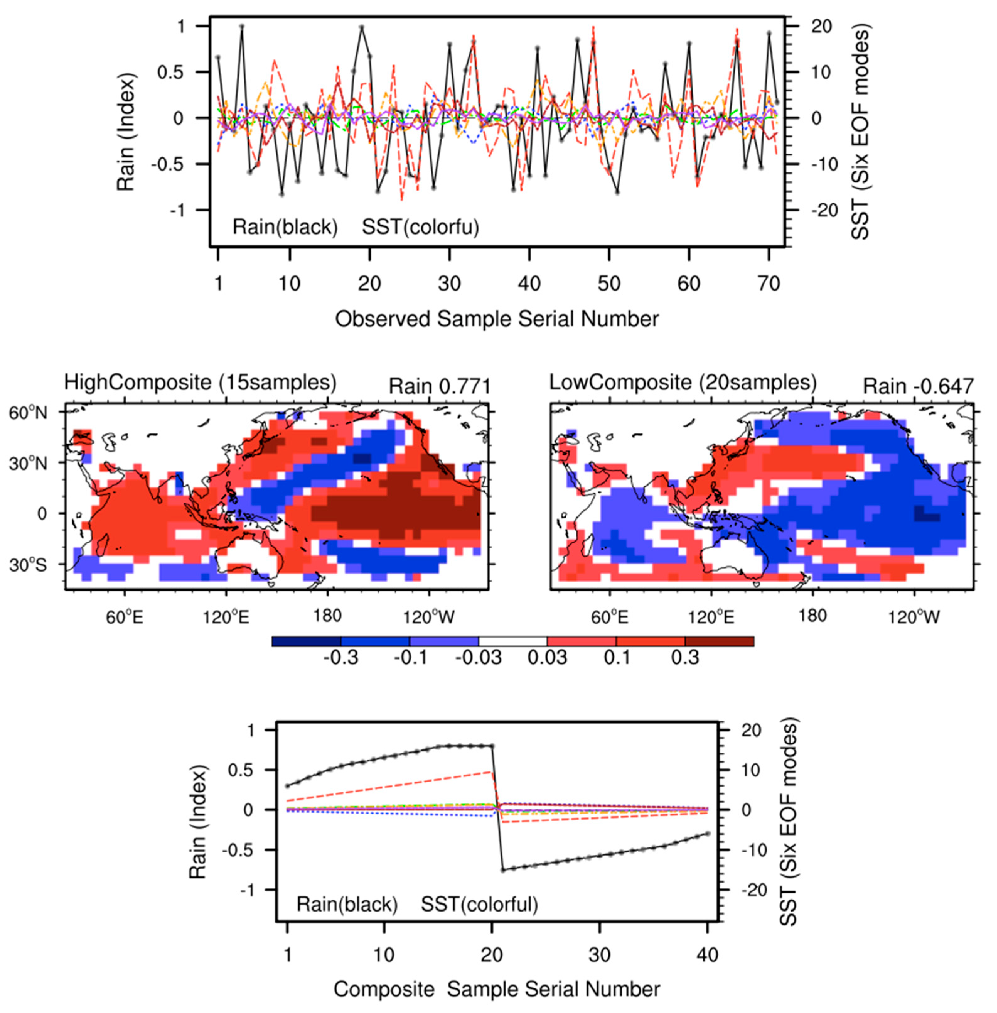
Figure 2.
Performance of 30 pre-trained models on composite samples (upper panel) and observed samples (lower panel). Rain from samples is represented by a black line, and that from the 30 models by 30 blue lines. The red line marks the curve that performs best among the 30 models for the former part of samples (1~45). The scores (Loss and Cor) include two components: the mean value and standard deviation of results from the 30 models.
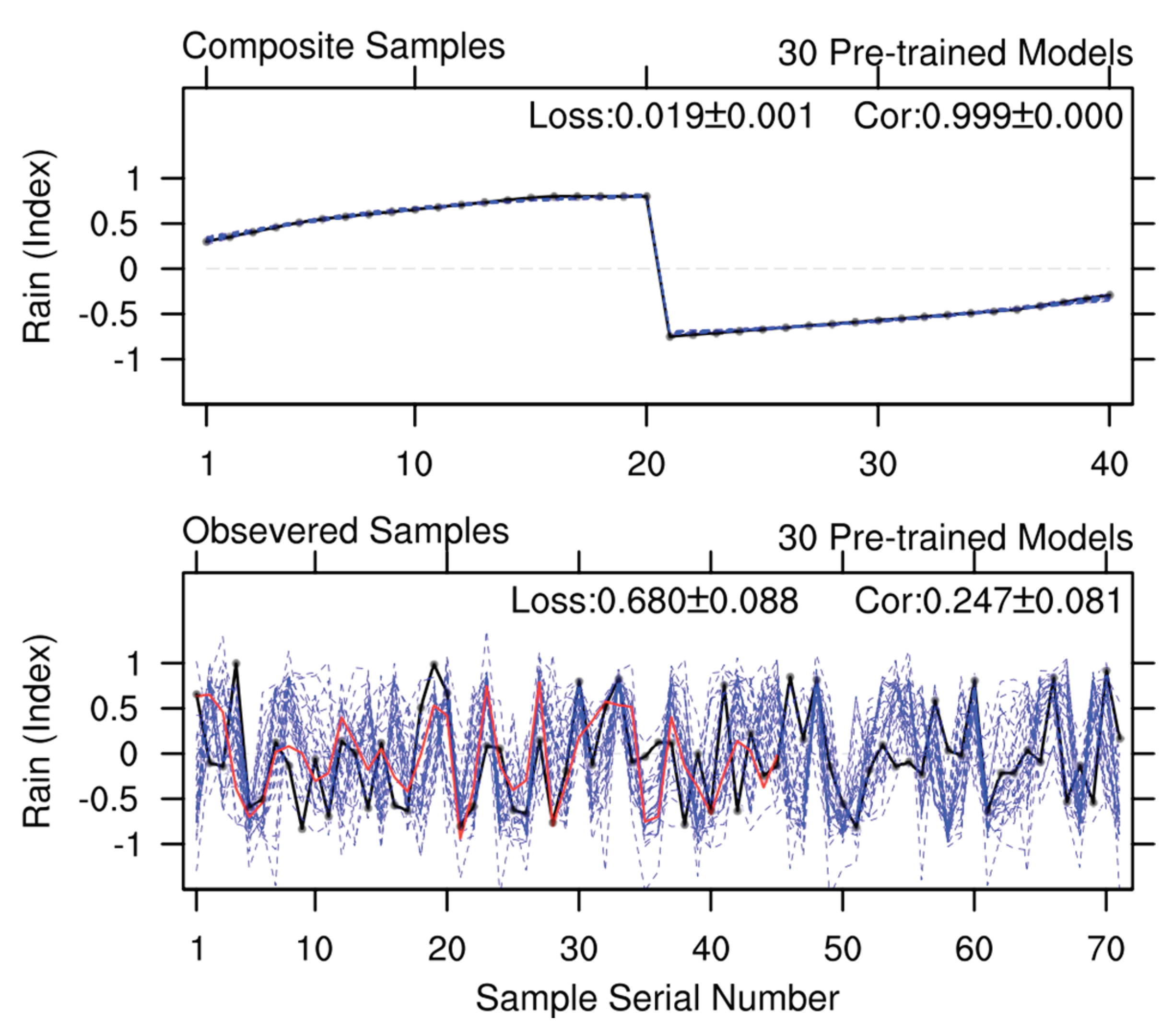
Figure 3.
Rain from observed samples (black line) and 30 model calculations (30 blue lines) across different model training approaches: without pre-trained models (upper panel), using different pre-trained models (middle panel), and using one fixed pre-trained model (lower panel). The upper part of each panel shows the scores of these models on the training set and test set, respectively.
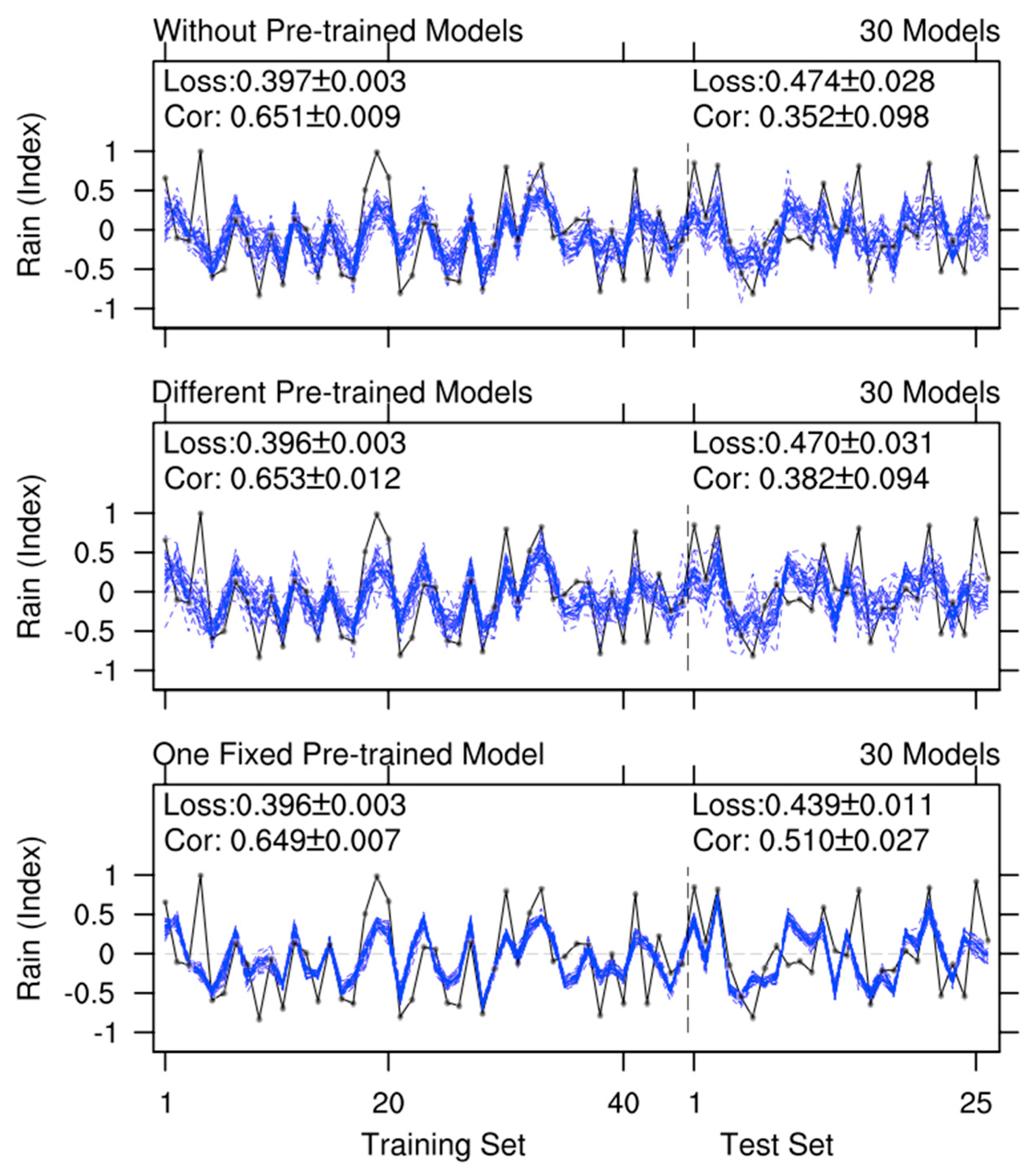
Figure 4.
Similar to Figure 3, but showing values from 10 groups of model ensemble experiments.
Figure 4.
Similar to Figure 3, but showing values from 10 groups of model ensemble experiments.
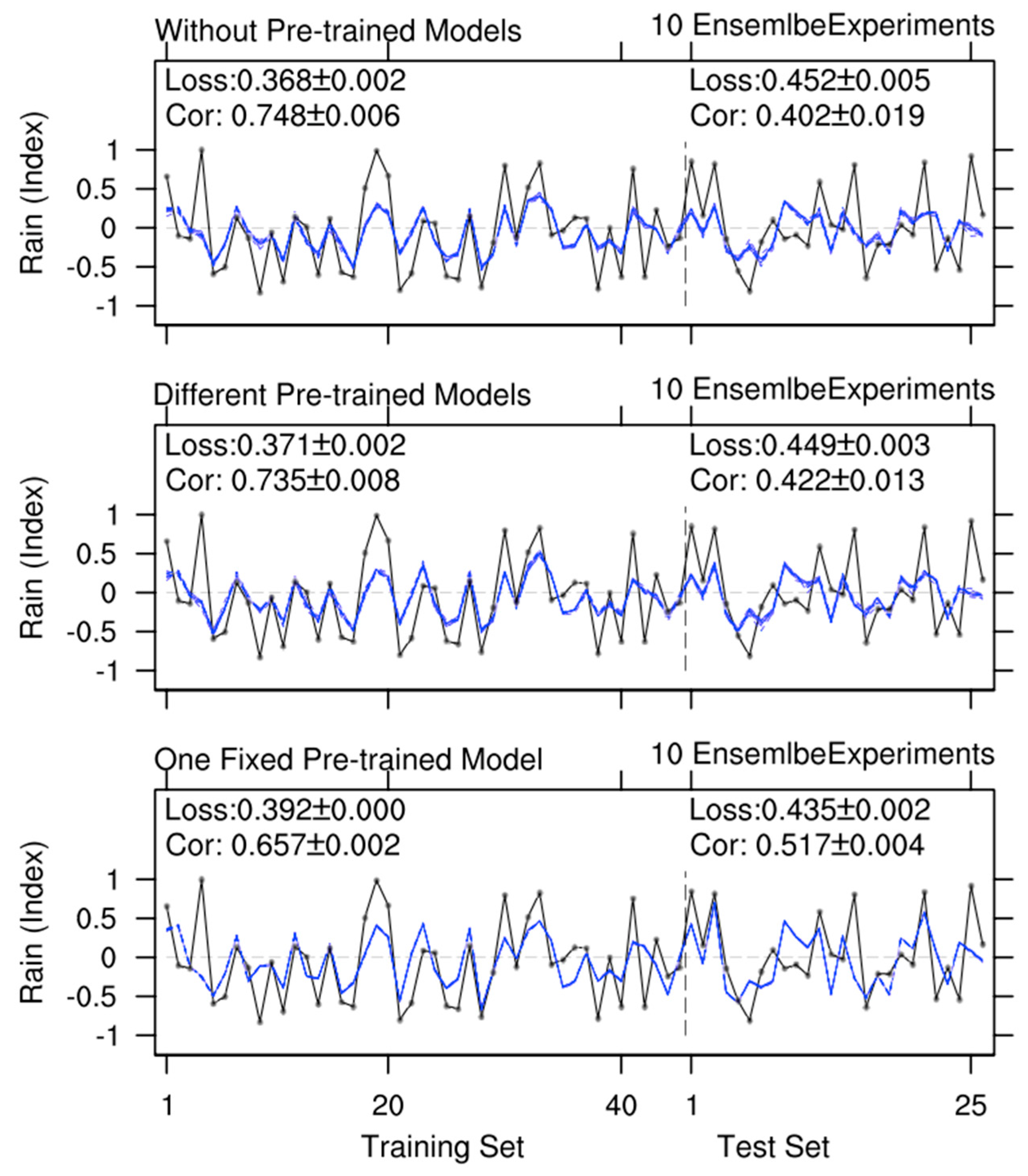
Figure 5.
Similar to Figure 4, but showing results of Leave-One-Out ensemble experiments on the test set.
Figure 5.
Similar to Figure 4, but showing results of Leave-One-Out ensemble experiments on the test set.
Disclaimer/Publisher’s Note: The statements, opinions and data contained in all publications are solely those of the individual author(s) and contributor(s) and not of MDPI and/or the editor(s). MDPI and/or the editor(s) disclaim responsibility for any injury to people or property resulting from any ideas, methods, instructions or products referred to in the content. |
© 2025 by the authors. Licensee MDPI, Basel, Switzerland. This article is an open access article distributed under the terms and conditions of the Creative Commons Attribution (CC BY) license (http://creativecommons.org/licenses/by/4.0/).
Copyright: This open access article is published under a Creative Commons CC BY 4.0 license, which permit the free download, distribution, and reuse, provided that the author and preprint are cited in any reuse.


