
Submitted:
10 November 2025
Posted:
12 November 2025
You are already at the latest version
Abstract
This study investigates the feasibility of a smartphone application that utilises the YOLOv11 object detection model to diagnose elbow fractures from X-ray images, motivated by the poor clinician performance in diagnosing these injuries. The investigation included training a YOLOv11 model on a labelled dataset of elbow fractures and deploying it on a mobile application. The application was capable of running inference on images loaded from the photo library, taking photographs for inference and running live inference using an image stream from the phone’s camera. The model achieved an average mAP@50 of 69.3% and an F1 score of 92.7% on radiograph scans, exhibiting overall poor results on both tests. Specifically, F1 scores ranged from 31% to 60.3% in the camera tests and from 28.8% to 43.1% in the live inference tests. The results suggest that for fracture detection to be reliably used with the phone’s camera, a diverse and high-quality dataset that accounts for different viewing conditions is required.
Keywords:
YOLOv11
; artificial intelligence
; fracture detection
; pediatric elbow fractures
; CNN
1. Introduction
Recent developments in artificial intelligence (AI), particularly deep learning, have shown significant potential in assisting clinicians with bone fracture detection and diagnosis. The research indicates that AI models, especially those using convolutional neural networks (CNNs), achieve diagnostic accuracy, sensitivity, and specificity comparable to or sometimes exceeding that of clinicians, suggesting AI can serve as a valuable adjunct in clinical practice [1,2,3]. Studies demonstrate that AI assistance improves clinicians’ sensitivity in detecting fractures, reduces diagnostic errors, and shortens reading times, thereby enhancing both the speed and accuracy of diagnosis in emergency and routine settings [3,4,5].
AI systems have proven effective across various imaging modalities (X-ray, CT, MRI) and body regions, and commercial AI algorithms have performed well in real-world emergency department scenarios [6]. However, challenges remain regarding clinical translation, regulatory approval, and ensuring model robustness and safety before widespread adoption [2,4]. AI holds great promise for improving fracture detection workflows and patient outcomes, but further work is needed to address implementation barriers and optimize integration into clinical practice [1,2,7]. Furthermore, the ability of clinicians to interpret X-ray images of elbow injuries remains inadequate, even in developed countries, and empirical data indicate an accuracy rate of only 54.4% for the correct diagnosis of children’s elbow injuries when clinicians are presented with a set of ten such images [8]. In contrast, models such as DenseNet-201 have achieved an accuracy of 94.1% in performing the same task [9].
Considering that in many low-income nations, there is a lack of access to immediate medical attention in some areas, communicating with a clinician via a smartphone has been demonstrated to be effective in obtaining a real-time diagnosis in emergency cases [10]. Research on integrating bone fracture detection models into smartphones and edge devices is currently scarce, but it demonstrates the potential for improving healthcare accessibility [11]. Despite the advancements in AI usage in medical imaging, generalisation is an issue many models face. This occurs when model performance declines when used to analyse the data of a patient who differs from the patient data used to train the model. For example, an AI model for detecting cervical spine fractures demonstrated poor real-world performance despite promising results during testing [12]. Other hurdles in this area also include model explainability, which is necessary for clinicians to understand the logic and reasoning leading to AI predictions in complex scenarios [13].
Rayan et al. address a critical issue in the preliminary assessment of radiographs, typically conducted by clinicians without specialization in radiology. These practitioners may lack the requisite expertise to discern complex fracture patterns unique to specific demographic groups, such as children or senior citizens, especially in high-pressure settings like emergency departments and urgent care facilities, where precise and rapid patient triage is crucial. In instances where immediate consultation with a radiologist is unfeasible, the implementation of an AI-based fracture detection system could substantially enhance the efficacy and accuracy of patient triage [14]. Delays or the absence of treatment for elbow fractures can result in long-term issues, including immediate complications such as nerve palsy, joint immobility, and cubitus varus, a condition marked by improper alignment of the elbow joint [15]. The gravity of these conditions underscores the importance of having tools that can increase the speed and accuracy of diagnosing elbow fractures.
This article aims to identify and evaluate the feasibility, in terms of performance, accuracy and usability of AI models deployed in mobile devices and their application for interpreting elbow X-ray images in a clinical setting, using a Convolutional Neural Network (CNN) model for real-time image interpretation.
This article is structured as follows: In Section 2, we review prior work focused on defining and utilizing fracture detection methods for mobile devices. Section 3 details the experimental setup for real-time detection of fractures. Section 4 presents the results, including a critical discussion. Finally, Section 6 concludes the article, offering suggestions for future research.
2. Related Work
Medical imaging technologies, including MRI, X-ray, and PET scans, are essential to modern diagnostic healthcare. Although critical, clinician interpretations can be affected by fatigue, cognitive biases, and variability in proficiency, leading to inconsistent diagnoses [16]. Artificial intelligence addresses these challenges by enhancing diagnostic precision through its pattern recognition abilities, detecting minute details beyond human capability, speeding up data analysis, and reducing healthcare costs by optimizing resources [16,17]. Recent AI applications in medical imaging have highlighted significant progress, particularly in cancer detection. CNNs have demonstrated efficacy in detecting brain tumours from MRI and PET scans, improving liver and pancreas imaging through accelerated segmentation and scanning, and enhancing breast cancer detection accuracy with limited training data [13].
2.1. Bone Fracture Detection
Artificial intelligence has shown remarkable proficiency in identifying bone fractures, with CNN-based models regularly outperforming human radiologists in terms of accuracy, sensitivity, and specificity[12]. The relevance of this technology is highlighted by the fact that misdiagnosed bone fractures account for roughly 80% of medical errors in emergency departments, a challenge intensified by the increasing scarcity of radiologists due to hiring delays and workforce attrition [18]. Investigations over the past twenty years indicate that AI models offer high classification accuracy, featuring an average sensitivity rate of 92%, while radiograph-based detection achieves a pooled sensitivity of 94% [2]. Several strategies have been pursued to enhance fracture detection models. The incorporation of attention mechanisms, which enable models to focus on crucial areas of input data, has improved detection efficiency [12]. Transfer learning, involving the refining of models pre-trained on extensive datasets for fracture detection purposes, has shown noteworthy accuracy with minimal need for specialized data [19]. Recent research applying YOLOv8 for the quality control of elbow radiographs has demonstrated the methodology’s high performance in terms of evaluation time, precision, and recall, as well as its capability to identify distinct elbow joint elements [9]. An analysis of detection frameworks highlights significant trade-offs. One-stage frameworks, such as YOLO, which function as a Single Shot Detector (SSD), require considerably fewer computational resources and offer greater speed than two-stage frameworks, albeit at the cost of reduced accuracy. Although specific studies claim that YOLO is unmatched in speed, comprehensive reviews present a nuanced view, suggesting that YOLO is ideal for speed-focused applications, while recommending models such as Faster R-CNN or RetinaNet for high accuracy and effective detection of small objects. CT scans have been shown to be more accurate than X-ray images, achieving up to 100% sensitivity in specific scenarios, compared to the 75.2% observed with AI-aided X-ray fracture detection. Additionally, an evaluation of BoneView, a commercially available AI diagnostic tool, indicated that it enhanced radiologists’ sensitivity and negative predictive value for wrist and hand fracture detection by an average of 5.3% at the patient level, enabling junior radiologists to match the diagnosis accuracy of their senior peers when utilizing the tool [18].
2.2. Elbow Fracture Challenges
Bone complexity and specificity tailored to a patient contribute to up to 11% of acute fractures being missed by physicians in emergency settings compared to trained radiologists. The situation is particularly problematic in high-volume emergency departments and urgent care centres where pediatric radiologists may not be readily available, making accurate and efficient patient triage paramount [20]. Concealed fractures pose a significant diagnostic challenge, as they may only be visible from specific angles or X-ray views. The relatively smaller size of bones in children and smaller individuals reduces image clarity. Models using DenseNet-201 could detect such fractures with 94.1% accuracy and 98.7% AUC during training, achieving 90.5% and 89.3% accuracy in external validation—superior to other compared models [9]. The clinical importance of accurate diagnosis is emphasized by potential long-term consequences of missed or delayed treatment, including nerve palsy, joint stiffness, and cubitus varus (elbow joint misalignment) [18]. Meta-analysis of six studies examining deep learning models for elbow injury detection revealed high performance metrics with pooled sensitivity of 0.93, specificity of 0.89, and AUC of 0.95, suggesting these models could reliably screen patients in busy emergency settings [15].
2.3. Current Approaches
In recent years, various artificial intelligence (AI) methods and strategies have been explored to enhance the identification of fractures in pediatric elbows. These approaches have evolved from leveraging two distinct deep convolutional neural network (CNN) models, which generate heatmaps to assist clinicians by utilizing an extensive dataset comprising 1,956 pediatric elbow x-rays, assessed by a panel of eight radiologists. The study observed that the efficacy of AI models in enhancing or impairing diagnostic performance is contingent upon the specific model employed [21]. DenseNet-201, for instance, was implemented for diagnosing elbow fractures, achieving an accuracy of 94.1% [9]. Nevertheless, this model demonstrated lower precision and recall relative to others, with VGG16 emerging as the superior performer among the examined deep convolutional neural networks (DCNNs) [22]. Recent advancements have extensively investigated YOLO variants for fracture detection. For instance, the application of YOLOv8 to pediatric wrist injuries attained a precision of 77.80% [23]. In other studies, the introduction of ghost convolutions to YOLOv11 facilitated an inference time of 2.4 ms, achieving a mean Average Precision (mAP) of 53.5% at an Intersection over Union (IoU) threshold of 0.5 on the GRAZPEDWRI-DX dataset [24]. However, evaluations of YOLOv9, replicated in [9], reported mAP scores of 65.46% at IoU=50 and 43.73% at IoU=50-95, challenging previous benchmark assertions [24]. These investigations highlight the profound impact of dataset quality and diversity on detection models, with significant implications arising from the limited representation of bone anomalies and soft tissue data in the GRAZPEDWRI-DX dataset. Altmann-Schneider et al.’s evaluation of the BoneView algorithm for the most prevalent fractures (forearm, elbow, lower leg) involved 1,000 radiographs for each body part. For elbow radiographs, where the average patient age was 7.7±3.7 years with a gender ratio of 55% male to 45% female, classifying dubious cases (50-90% confidence) as fractures achieved a sensitivity of 91.5% but specificity of 63.7%. When these were classified as non-fractures, sensitivity decreased to 80.5%, while specificity increased to 94.9%. This underlined the need for further refinement for dependable clinical implementation [25]. Dupuis et al. validated Milvue’s AI algorithm, observing a negative predictive value of 92%, although they identified methodological shortcomings, as the assessment focused on agreement with radiologists rather than genuine diagnostic performance [20]. Multiple studies emphasize the pivotal role of high-quality, diverse datasets, asserting their necessity for optimizing model performance. Kutbi illustrated that high-quality annotated training sets—although currently rare and costly to develop are essential for producing robust models across diverse populations and imaging modalities [2]. A study conducted by Zech et al. further corroborates this, showing that an open-source pediatric fracture detection algorithm (childfx.com) substantially augmented diagnostic accuracy for both physicians and radiologists, enhancing physician sensitivity from 0.842 to 0.858 and radiologist sensitivity from 0.781 to 0.883. The findings suggest that AI integration predominantly bolsters the performance of less specialized and experienced interpreters, bringing their diagnostic capabilities closer to those of subspecialists [26].
2.4. Application in Mobile and Edge Environments
Despite extensive research on fracture detection, limited work addresses the integration of smartphones and edge devices [27]. MobileNet appears to be the most researched in this domain, with a CNN architecture designed for mobile devices that minimises parameters to accelerate computation at the cost of reduced efficiency compared to other deep CNNs [28]. Studies involved an analysis of MobileNetV2 for bone fracture detection using MobileNetV2 tested alongside other CNN architectures such as VGG16, ResNeXt, AlexNet and SFNet. The results outline inconclusive outcomes, showing conflicting results for MobileNetV2, with a range of 59% F1 score to 48% accuracy, compared to models that achieve 93.5% accuracy as outlined in [28] and [29]. Furthermore, a comparison of MobileNetV3 with ResNet50 using the MURA dataset (20,335 images across elbows, hands, and shoulders) found that MobileNetV3 achieved 78.37% accuracy for elbow fractures, versus ResNet50’s 76.83%, indicating that MobileNetV3’s fast inference times make it viable for real-time clinical applications on smartphones and tablets [27].
Despite the fact that the research using non-MobileNet object detection models for bone fracture detection from radiographs on edge devices is generally lacking, a comparison of MobileNetV2 against YOLO-X for obscured facial recognition found that YOLO-X outperformed across accuracy, precision, recall, and F1 score, suggesting YOLO could be a suitable candidate for mobile fracture detection deployment [30].
Despite AI’s demonstrated capabilities, high-quality, diverse datasets accounting for varied populations, rare fracture types, different viewing angles, lighting conditions, and camera distances remain scarce. The quality of the dataset fundamentally determines model performance and its real-world applicability. While CNNs show promise for clinical elbow X-ray diagnosis, research lacks evaluation of system requirements, resource usage, and actual smartphone and edge efficiency for these models. The feasibility of smartphone and edge applications for real-time clinical assistance remains unexplored, representing a significant opportunity to improve healthcare accessibility in resource-limited settings and emergency departments.
3. Materials and Methods
This section elaborates on and analyzes the design decisions made in the experimental setup. The experiment is structured into four phases, with each focusing on distinct elements of the design. The initial phase encompasses data preparation and model training methodologies, while the subsequent phase involves exporting the Yolo model and developing the application. The third phase is dedicated to implementing particular app features, as well as the associated evaluation and testing. The verall pipeline is outlined in Figure 1.
3.1. Data Preparation and Model Training
The foundation for the entire fracture detection system goes through careful dataset preparation and systematic model training. The process begins with acquiring a labelled dataset from Roboflow containing approximately 1,100 adult elbow X-ray images. This dataset contains YOLO-formatted annotations with bounding box coordinates and binary classifications (fractured vs. non-fractured). A critical step involves reorganizing the dataset into two different split configurations: an 80/10/10% and a 70/15/15% distribution across training, validation, and testing subsets. The dual-split strategy enables a comparative analysis of how different training/validation/testing ratios impact model performance, which is particularly important given the relatively small dataset size. The training methodology emphasizes rigorous hyperparameter optimization using Optuna, an open-source framework that automates the search for optimal model configurations. Over 60 trials, the system explores combinations of five critical hyperparameters outlined in Table 1.
The choice of a random search algorithm provides computational efficiency while avoiding the curse of dimensionality that would plague exhaustive grid search approaches. This optimization targets the mean F1 score across both classes, balancing precision and recall rather than optimizing for accuracy alone—a crucial decision given the clinical context where both false positives and false negatives carry significant consequences. The training process incorporates an early stopping mechanism with a patience parameter of 10 epochs, allowing the model to train up to 1,000 epochs but automatically halting when validation metrics plateau, thereby preventing overfitting while maximizing learning from the limited dataset. The rationale for this comprehensive approach stems from fundamental machine learning principles and the specific constraints of medical imaging applications. The dataset split experimentation acknowledges that with only 1,100 images, the allocation between training and validation data significantly impacts model generalization—too little validation data yields unreliable performance estimates, while too little training data hampers learning. The emphasis on hyperparameter tuning through automated optimization rather than manual adjustment ensures reproducibility and objectivity, particularly important for medical AI applications that face scrutiny regarding methodology. Furthermore, the selection of YOLOv11 as the base architecture aligns with the project’s dual requirements: achieving clinical-grade accuracy comparable to state-of-the-art models while maintaining computational efficiency suitable for smartphone deployment. This phase ultimately produces two distinct models (Model 1 and Model 2) trained on different data splits, enabling empirical comparison of how dataset allocation affects real-world performance in subsequent testing phases.
3.2. Model Export and Deployment
Phase 2 represents a critical transition from research-grade model training to practical mobile deployment, where the trained YOLOv11 models must be converted into a format optimized for resource-constrained smartphone environments. TensorFlow Lite (TFLite) was chosen as the deployment format after evaluating three potential options: PyTorch (with ExecuTorch), ONNX Runtime, and TFLite with LiteRT. This decision was informed by TFLite’s superior performance characteristics—being smaller, faster, and offering better hardware acceleration compared to alternatives. The export process, executed through Ultralytics’ which transformed the PyTorch-trained models into mobile-optimized TFLite versions. Critically, the FP16 quantization was enabled during export, which compresses model weights from 32-bit to 16-bit floating points, reducing model size by approximately 50% while maintaining acceptable accuracy, a crucial optimization for mobile devices with limited storage and memory.
The crucial step in this phase is to properly understand and map the output from a trained YOLOv11 model, which utilises Non-Maximum Suppression (NMS) for object detection during model training. Since detection models tend to output a large number of possible detections, this often results in many overlapping bounding boxes. Non-Maximum Suppression (NMS) helps to interpret these outputs by combining object detection bounding boxes that appear to belong to the same object. This helps to remove redundant object detection information. The NMS implemented in YOLO uses a recursive approach by doing score thresholding, i.e. removing bounding boxes with a confidence score below a specified threshold; sorting the remaining bounding boxes in descending order of confidence (sorting by confidence) and iterative selection and suppression by finding the intersection over Union (IoU) where the overlap of two bounding boxes occurs. IoU is calculated as:
where the describes the area where two boxes intersect, while the describes the total area the two boxes occupy. The IoU of the bounding box with the highest confidence score is checked against the remaining boxes, which are then removed if they fall above a specified threshold. If other bounding boxes overlap sufficiently with the chosen bounding box, they are also removed.
3.3. Application Features Implementation
The application’s features were designed with clinical practicality and user accessibility in mind. The following three distinct inference pathways were implemented to accommodate different real-world usage scenarios:
- Loading images from a photo library to enable the classification of pre-existing saved radiographs.
- Direct camera capturing to allow for immediate fracture classification.
- Live fracture detection that provides real-time feedback during positioning and imaging.
This multi-modal approach ensures flexibility in clinical workflows, whether reviewing archived images or conducting point-of-care assessments.
The single-page UI/UX design with colour-coded results (blue for non-fracture, red for fracture) was deliberately chosen to minimise cognitive load and enable rapid visual interpretation by healthcare providers. Large buttons and clear text enhance accessibility across diverse user groups and lighting conditions, while guideline-based responsive constraints ensure consistent functionality across various Android devices with varying screen sizes.
3.4. Evaluation and Testing
The evaluation strategy was structured to assess both technical performance and real-world applicability through progressively challenging testing scenarios. Model output processing prioritized the highest confidence prediction after Non-Maximum Suppression filtering to reduce false positives and provide clinicians with the most reliable assessment. Dual metrics—classification measures (precision, recall, f1-score) and detection metrics (IoU, mAP)—were employed to comprehensively evaluate both the diagnostic accuracy and spatial localization capability of the system.
Precision measures the proportion of correctly predicted positive results out of all positive predictions made, and it is calculated as:
where is the true positive rate and is the false positive rate during model prediction.
Recall is the ratio of true positive predictions to the total number of actual positive cases and is given as:
where is the true positive rate and is the false negative rate during model prediction.
The f1-score is the harmonic mean of precision and recall, calculated to provide a single score that balances recall and precision. The f1-score is given as:
The detection metric utilized is (earlier explained in Section 3.2), along with mean average precision (). The mean Average Precision serves as a common standard for assessing the efficacy of object detection models. The methodology of calculation involves filtering predictions with 0% confidence, ranking them by confidence using NMS, and assessing each based on its against a set threshold to categorize as true or false positives/negatives. Sorted predictions were used to plot the PR curve, calculating precision and recall iteratively to evaluate object detection model performance.
This methodology yielded a series of precision-recall pairs, facilitating the plotting of the curve and enabling the computation of through the integration of the area beneath the curve. This was achieved using the Riemann sum:
where is the precision value at index i, , and denotes the recall at position :
Finally, the testing scenarios progressed from controlled conditions using the standard test set, to an independent Google Images dataset that simulates varied image quality, to physically printed radiographs under different lighting and angular orientations. This final testing phase with printed X-rays was particularly critical as it mirrors actual deployment conditions where users would photograph existing radiographs rather than directly inputting digital DICOM files. Performance benchmarking across emulated devices with varying RAM capacities (4GB to 12GB) ensured the application would function efficiently on both older and newer smartphones, addressing the practical constraint that not all clinical settings have access to high-end devices.
4. Results
The findings detailed in this section follow the sequential steps set forth in the design Section 3.
4.1. Model Training Results
Five best hyperparameters were used to search the parameter space for both models (Model 1 and Model 2).

Table 2.
Best hyperparameter values used for model training for Models 1 & 2.
| Hyperparameter | Model 1 | Model 2 |
|---|---|---|
| Initial Learning Rate (lr0) | 0.0810 | 0.0492 |
| Final Learning Rate (lrf) | 0.8947 | 0.3719 |
| Batch Size | 32 | 32 |
| Box Loss Weight | 0.1610 | 0.1043 |
| Classification loss weight | 0.9062 | 0.5831 |
Before exporting, the two trained models were evaluated using their respective testing subsets, where model predictions were tested against ground truths on the test set.
Table 3.
Summary of post-training performance metrics of Models 1 & 2. Further results can be found in table A.9 in the appendix.
Table 3.
Summary of post-training performance metrics of Models 1 & 2. Further results can be found in table A.9 in the appendix.
| Performance Metric | Model 1 | Model 2 |
|---|---|---|
| Average precision | 0.821 | 0.85 |
| Average recall | 0.89 | 0.722 |
| Average mAP50 | 0.878 | 0.814 |
| Average mAP50-95 | 0.408 | 0.375 |
| Average F1 Score | 0.854 | 0.781 |
Overall, the models displayed satisfactory results, with reliable F1 and mAP scores. Model 1 demonstrated an advantage over Model 2 across most metrics.
Model 2 displayed a comparable F1 score to Model 1’s in terms of non-fracture detection, with the former scoring 93.7% and the latter 94%. Both models demonstrated decreased performance in terms of fracture detection, with Model 1 achieving an F1 score of 79.7% and the 70/15/15 split model achieving 68.9%. This suggests that the model is designed to detect non-fractures. This can potentially be explained by the imbalance in the dataset, as two-thirds of the images in the training set were non-fractures, while one-third of the images were fractures.
Furthermore, the precision-recall curves for both models indicate a good AUC for both models, resulting in 87.8% for model 1 and 81.4% for model 2, respectively. Figure 2 illustrates the PR curves for both models.
If we analyse the AUC class-wise (fracture and non-fracture), we can also witness relatively high AUCs. For example, for the ’fracture’ class, the AUCs range from 59.2% for Model 2 to 81.6% for Model 1. Whilst for the ’non-fracture’ class we observe higher results with 94.0% for Model 1 and 93.7% for Model 2, respectively.
4.2. In-App Test Set Results
The tests outlined for calculating the metrics were repeated for both FP32 and FP16 versions of models 1 and 2 inside the developed application. Table 4 depicts the performance metric for Model 1 & 2 in terms of average f1-score, average accuracy, mAP@50, mAp@50-95 and confidence. The complete summary of in-app model performance. Further results can be found in Table A10 in the appendix.
Across testing, both models produced virtually identical results for their FP16 and FP32 versions, except that model 1’s FP16 version showed slightly higher mAP@50 and mAP@50-95 values. This difference could possibly have been caused by slight differences in bounding box coordinates and confidence scores arising from converting 32-bit floating points to 16-bits. Although other metrics would not pick up on this, mAP@0.5 and mAP0.5-0.95 are susceptible to being affected by these minute variations between models.
Compared to the pre-export results, both models demonstrated higher F1 scores across both classes, while mAP@0.5 and mAP@0.5-95 values decreased. The increase in F1 appears to stem from a general improvement in precision and recall across both classes. This, in turn, most likely stems from differences in confidence score handling: YOLO models use a default confidence threshold of 25% for a detection to be considered successful, whereas in models 1 and 2 the threshold was 0%. This means that some low-confidence predictions, although correct, would have been misclassified by the YOLO model, whereas they would have passed in models 1 and 2. This is further evidenced by the mAP scores, which take into account both confidence and bounding box coordinates. These metrics have deteriorated in models 1 and 2 relative to the pre-export model - this behaviour could be explained by the introduction of NMS into the exported models. NMS affects which bounding boxes the model keeps, which can indirectly affect predicted bounding box coordinates and confidence scores, leading to a decrease in mAP.
It is also important to note that the accuracy for both models was high: model 1 achieved 93.4% and model 2, 92.2%.
Figure 3.
PR Curves for each model, deployed in-app: (a) Precision-Recall Curve for Model 2 - FP16. (b) Precision-Recall Curve for Model 2 - FP32. (c) Precision-Recall Curve for Model 1 - FP16. (d) Precision-Recall Curve for Model 1 - FP32.
Figure 3.
PR Curves for each model, deployed in-app: (a) Precision-Recall Curve for Model 2 - FP16. (b) Precision-Recall Curve for Model 2 - FP32. (c) Precision-Recall Curve for Model 1 - FP16. (d) Precision-Recall Curve for Model 1 - FP32.
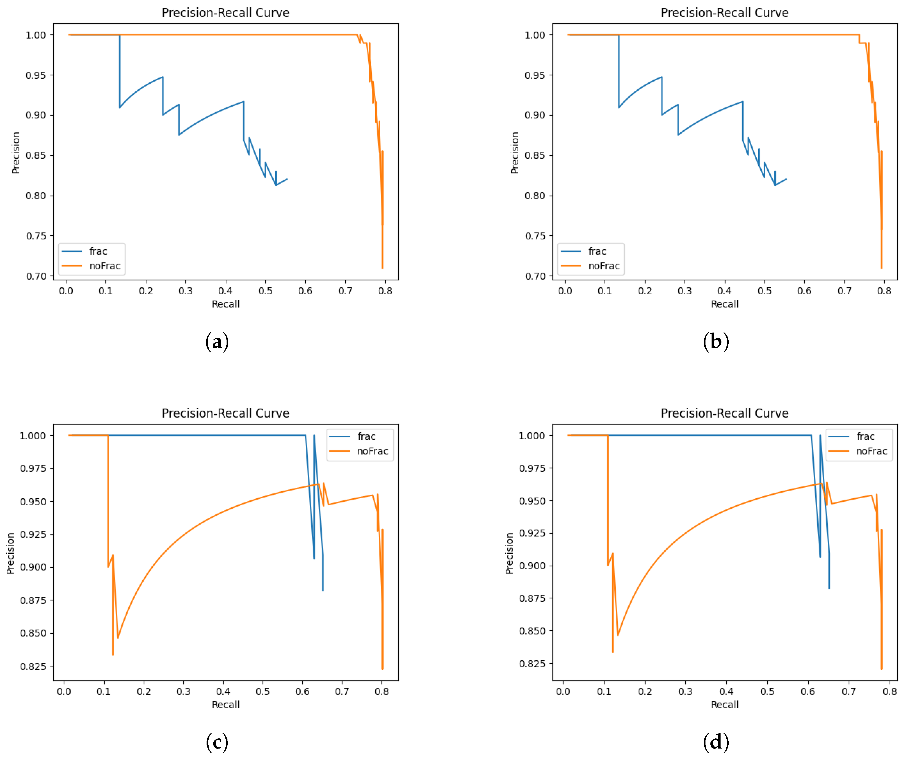
Precision-recall (PR) curves were constructed for the four computational models under analysis. It was observed that the graphical representations for the two versions of each of two specific models were nearly indistinguishable. The graphical data indicate that Model 2 exhibits a more advantageous non-fracture-detection curve, whereas Model 1 demonstrates a superior overall curve. Furthermore, Model 2 shows a more pronounced decline in precision across both prediction classes in comparison to Model 1. These observations are consistent with the results presented in Table 3, which indicate that Model 1 performs better overall than Model 2. The authors critically acknowledge several issues attributable to the limited number of instances in the dataset. Notably, the fracture class exhibits signs of overfitting in certain instances, and the dataset is characterized by class imbalance alongside relatively robust generalizability. To address these concerns, an independent evaluation of the models is undertaken as detailed in Section 4.2.1.
4.2.1. Independent Testing
To confirm the results of the previous experiment, the same test was run to calculate the model’s accuracy, recall, precision, and F1 score using an independent test set collected from Google Images. This set contained 10 images, 5 of fractured elbows and 5 of non-fractured elbows, and was intended to confirm the results of the previous test. Mean area precisions and bounding box values were not evaluated due to a lack of expertise in correctly identifying the areas of interest in diagnosing elbow fractures, which is required to correctly label bounding boxes.
The FP16 and FP32 results were consistent across both models, allowing for consolidated data analysis. Unlike previous testing, Model 2 demonstrated superior performance compared to Model 1, achieving average F1 and accuracy of 88.9% and 90%, respectively, whereas Model 1 attained 69.7% and 70%, respectively.
Table 5.
Summary of independent testing results for Models 1 & 2. Further results can be found in Table A11 in the appendix.
Table 5.
Summary of independent testing results for Models 1 & 2. Further results can be found in Table A11 in the appendix.
| Performance Metric | Model 1 FP32 & FP16 | Model 2 FP32 & FP16 |
|---|---|---|
| Average F1 Score | 0.697 | 0.889 |
| Average Confidence | 0.682 | 0.625 |
| Average Accuracy | 0.7 | 0.9 |
Although the test set utilized in this experiment is relatively small, potentially affecting the reliability of the results, the data suggests that both models have a certain degree of efficacy in making predictions on datasets outside their original training data. However, the performance discrepancy raises questions about the models’ generalizability. Specifically, Model 1, despite previous success, was outperformed by Model 2 on this independently gathered dataset. This finding underscores the importance of incorporating diverse training sets to ensure the generality and robustness of fracture detection models. Such diversity is crucial for improving model performance across varying datasets and enhancing the predictive accuracy of machine learning applications in this domain.
4.2.2. Performance Testing
For performance testing, Google Pixel devices were used to emulate the mobile app with varying amounts of RAM, which should help to approximate performance. For the purpose of this experiment, two smartphones were emulated: Pixel 3 (4GB RAM) and Pixel 8 Pro (12 GB RAM). To get an appropriate performance test, the possible user journeys were considered. The three main identified ones were:
- User launches the app, takes a photo with the camera and chooses it for model inference.
- User launches the app, selects a photo from the library and chooses it for model inference.
- User launches the app and starts live detection for model inference.
Seeing as the first and second journeys are quite similar, only the first one is out of the two was chosen for benchmarking, especially since it would be more resource-intensive than the second one due to the user taking a photo with the phone’s camera. Table 6 and Table 7 show resource usage (RAM and CPU) for both journeys.
Journey 1 exhibited an overall low CPU and RAM usage, utilising under 0.2 GB RAM and less than 4% of the CPU.
Journey 2 demonstrated increased resource usage from Journey 1, specifically with the CPU usage rising approximately 20%.
It can be seen that for each journey the resource usage on both emulated devices differed by small amounts. Overall, using the live camera for object detection used more resources than taking a photo, using almost twice as much RAM and approximately six times the CPU power. This was expected, considering that for each second of live detection, multiple images from the camera are analysed, whereas for taking photographs, the model processes only one image for the whole use case.
The RAM usage for both journeys was relatively small, utilising less than half a gigabyte. This implies that even low-end devices with limited RAM can run the application without issues.
The CPU used for this experiment was an Intel i7-12700K, with a clock speed of 3610Mhz and 12 cores. Although this CPU is considerably more powerful than the CPUs used in smartphones, the fact that usage remained below 25% for both journeys implies that this application should run smoothly on most modern Android devices.
4.3. Real Camera Testing
In this segment of the experimental procedure, we assessed the application’s ability to capture images and perform inferential analysis on them. Model 1, demonstrating superior performance on the test dataset, was exclusively utilized for this task. A selection of ten images from the test subset was made, comprising five fracture and five non-fracture images, which were subsequently printed on standard A4 paper. Following this preparation, the application was executed on an emulated Pixel 8 Pro device, mirroring the configuration used during performance evaluations, with a computer webcam serving as the device’s emulated camera. Given its superior performance in prior evaluations, Model 1 was preferred over Model 2 for this task, and both its FP16 and FP32 versions were evaluated.
The model’s ability to accurately interpret printed images was evaluated using metrics such as accuracy, precision, recall, and F1 scores. To conduct a comprehensive analysis of the model’s robustness, images were captured under varied lighting conditions, including natural daylight and artificial illumination, and from different perspectives: directly overhead, at a 45-degree angle from the paper, and at a 45-degree lateral angle. Figure 4 outlines some of the correctly classified cases from image radiographs.
A successful identification of a specific category was considered a true positive. Conversely, an incorrect classification was defined as a false negative for the correct category and a false positive for the incorrectly identified category. For instance, should a fracture be misidentified as a non-fracture, it was logged as a false negative for the fracture category and a false positive for the non-fracture category. In scenarios where no identification was achieved after three photographic attempts, this was deemed a false negative for the intended detection category. The initial category identified was consistently recorded as the definitive outcome.
Although bounding boxes were not quantitatively verified, if a prediction showed a bounding box outside of the general elbow area in the image, the prediction was not counted as a true positive.
The results from the above tests can be summarised as follows:
Table 8.
Summary of model inference results from phone camera photos. More details are in Table A1–Table A4 in the appendix.
| Model | Lighting | Avg. Precision | Avg. Recall | Avg. F1 Score |
|---|---|---|---|---|
| 80/10/10 FP32 | Daylight | 0.669 | 0.533 | 0.549 |
| 80/10/10 FP32 | Artificial | 0.563 | 0.5 | 0.516 |
| 80/10/10 FP16 | Daylight | 0.653 | 0.625 | 0.603 |
| 80/10/10 FP16 | Artificial | 0.334 | 0.3 | 0.31 |
The model experienced an acute decrease in precision and recall when running inference on photos of radiographs instead of scans, such as in the previous experiments. This result makes sense, as the model was trained on radiograph scans and not photos taken of radiographs, which can introduce variety in angles, lighting and object distance, affecting both model training and post-training performance. Furthermore, many of the radiograph results were inconsistent, with the angles and lighting affecting model prediction for each radiograph. Figure 5 outlines the mode’s inconsistent detection at various leading to various confidence levels resulting to false positives and negatives respectively.
For both versions of the model, there was a clear decrease in both precision and recall when artificial lighting was used over natural lighting - this points to the importance of strong and clear lighting when using the camera for radiograph inference.
These results suggest that for inference to be run on radiograph photographs, a more robust training set is required, and should consist of both scans and photographs of radiographs, including various angles and lighting conditions. This could potentially allow the model to have more consistent and accurate results.
4.4. Live Detection Testing
The app’s ability to dynamically detect objects in-app using the phone’s camera was tested for this part of the experiment. The same setup was used as in the camera testing. As in this case, it was not just one image being analysed, but rather a constant stream; the most prevalent detection was accepted as the model prediction in each testing scenario. If a model’s prediction did not stabilise for an image from a given angle, it was counted as a false negative. Figure 6 illustrates some of the examples of successful live predictions.
Table 9 illustrates the model’s live inference performance provided through their respective average precision, recall and F1 score values.
Following the previous testing using camera photographs, the application’s live detection feature displayed a further decrease in precision, recall, and average F1 score across both model versions. This result could have been expected, as a constant image stream includes further variations in angles, lighting, and radiograph distance, which can result from slight hand movements. Figure 7 depicts the inconsistencies in live detection under the same lighting conditions viewed from the same angles.
The model’s inconsistent behaviour was also exacerbated, providing constantly changing predictions, even when the angle, lighting and distance stayed relatively unchanged. This calls into question not just the model’s reliability, but also whether live fracture detection is a feature that makes sense in the context of assisting clinicians in fracture diagnosis. To further examine this, a training set consisting of video footage of radiographs, containing labelled video frames, could help to improve model performance in this regard.
5. Discussion
This study investigated the feasibility of deploying YOLOv11-based elbow fracture detection on mobile devices, revealing both promising capabilities and critical limitations that must be addressed before clinical implementation. The research bridges laboratory model development with practical deployment considerations, exposing significant challenges in translating AI performance from controlled datasets to real-world mobile applications.
5.1. Performance on Digital Radiographs and Clinical Relevance
Model 1 achieved notable performance metrics on digital radiographs within the mobile application, with accuracy of 93.4%, F1 score of 92.7%, and mAP@50 of 69.3%. These results are competitive with current state-of-the-art systems, approaching the 94.1% accuracy reported by Li et al [9]. For pediatric elbow fracture detection using DenseNet-201 [9], while substantially exceeding the 53.5% mAP@50 benchmark established for pediatric wrist fracture detection [24]. Given that clinician accuracy for pediatric elbow fractures is only 54.4% [8], Model 1’s performance on digital radiographs demonstrates that AI could meaningfully augment clinical decision-making in controlled conditions. The superior performance of Model 1 (80/10/10 split) over Model 2 (70/15/15 split) underscores the importance of dataset allocation optimization, particularly with limited training data. However, both models exhibited class imbalance effects, achieving higher F1 scores for non-fracture detection (93.7-94%) compared to fracture detection (68.9-79.7%). This bias toward the majority class represents a significant clinical concern, as false negatives could lead to missed diagnoses and serious complications including nerve palsy, joint stiffness, and cubitus varus [15]. The dataset’s two-thirds non-fracture to one-third fracture ratio likely contributed to this disparity, suggesting future implementations should employ weighted loss functions or targeted data augmentation to prioritize fracture detection sensitivity.
Two models, model 1 and model 2, were tested for their ability to detect elbow fractures from radiographs. Model 1 displayed superior performance over model 2, with a mean accuracy of 93.4%, F1 score of 92.7% and mAP@.5 of 70.4% when tested on scans of radiographs inside of the Android application.
These results for accuracy are comparable with the current state-of-the-art for paediatric elbow detection, with Li et al. achieving an accuracy of 94.1% [9]. Furthermore, the mAP@0.5 score can be compared to the current benchmark of 53.5% for pediatric wrist fracture detection, as achieved by Ferdi [24].
The model displayed acutely diminished performance when using the phone’s camera for testing, with results heavily affected by camera positioning and lighting conditions. For fracture detection models to successfully detect fractures through this method, either by capturing photographs or using live detection, a high-quality, robust dataset created with this purpose is required.
The application’s resource usage was relatively low on emulated Android devices, suggesting that such fracture detection applications are feasible hardware-wise.
5.2. Generalization Challenges and Domain Shift
Independent testing revealed concerning variability in model performance. Model 2 achieved 90% accuracy on the Google Images test set compared to Model 1’s 70%; a reversal of their relative performance on the original test set. While the independent set was small (n=10), this finding suggests potential overfitting to specific characteristics of the training dataset, such as image quality, contrast levels, or institutional imaging protocols. This aligns with research by Kutbi [2] and Zech et al. [26] emphasizing that diverse, multi-institutional datasets are essential for robust clinical AI systems. The models’ vulnerability to distribution shifts highlights the necessity of training data that captures real-world heterogeneity in imaging equipment, exposure settings, patient positioning, and image processing pipelines.
5.3. Improoving the Performance Degradation in Camera-Based Inference
The most significant finding is the dramatic performance decline when models analyzed photographs of printed radiographs rather than digital scans. F1 scores plummeted from 92.7% to 31-60.3% for camera photographs and 28.8-43.1% for live detection. This precipitous decline stems from fundamental domain shift: models trained on consistent digital radiographs confronted photographs introducing ambient lighting variations, camera angles, distance effects, lens distortion, reflections, shadows, and motion blur. Our experiments demonstrated that environmental factors substantially impacted performance. Natural daylight generally yielded better results than artificial lighting, while 45-degree angle captures consistently underperformed overhead positioning. The live detection feature exhibited particularly poor stability, frequently alternating between fracture and non-fracture classifications for identical radiographs under unchanged conditions. This instability raises fundamental questions about whether continuous video-stream inference is appropriate for fracture detection tasks. These findings indicate that successfully deploying camera-based fracture detection requires fundamentally different training paradigms incorporating diverse data: radiograph photographs under varied lighting (natural, fluorescent, LED), multiple camera angles and distances, different surface reflectances, intentional blur and noise, and augmentation techniques simulating perspective transforms. Without such training data, camera-based inference remains unreliable for clinical deployment.
5.4. Computational Efficiency
A major contribution of this research is demonstrating that YOLOv11 models operate efficiently on mobile devices with modest hardware. Resource usage remained conservative: static image inference consumed under 0.2GB RAM and less than 4% CPU, while live detection required approximately 0.25GB RAM and 24% CPU. These demands suggest the application could function on budget Android devices with 4GB RAM, addressing accessibility concerns in resource-limited settings. FP16 quantization proved particularly valuable, reducing model size by 50% while producing virtually identical performance to FP32 versions across all tests. The minimal difference (e.g., Model 1’s mAP@50 of 70.4% for FP16 vs. 69.3% for FP32) validates aggressive model compression for mobile deployment. This computational efficiency, combined with YOLO’s single-stage detection architecture providing faster inference than two-stage detectors like Faster R-CNN, positions YOLOv11 as a viable architecture for real-time mobile medical imaging applications—if the domain shift challenges can be resolved.
6. Conclusions
The research makes important contributions: (1) demonstrating YOLOv11 can achieve clinically relevant accuracy while maintaining mobile-friendly computational requirements; (2) identifying the critical gap between laboratory validation and real-world camera-based performance; (3) quantifying environmental factors’ impact on model reliability; and (4) establishing that current training paradigms are insufficient for robust camera-based inference. Key strengths include computational efficiency, successful quantization, competitive accuracy on curated datasets, and systematic evaluation exposing critical limitations. Principal limitations center on inadequate dataset diversity, severe camera-based performance degradation, class imbalance favoring non-fracture detection, and absence of clinical validation. For reliable smartphone-based fracture detection, future work must develop diverse datasets explicitly incorporating varied viewing conditions, lighting scenarios, and acquisition contexts. Alternative approaches such as direct PACS integration or hybrid systems with uncertainty-aware inference may prove more viable. While this research demonstrates that AI-powered mobile fracture detection is technically feasible under controlled conditions, substantial innovations in domain-aware training, robust uncertainty quantification, and prospective clinical validation are required before such systems can safely assist clinicians in real-world settings. The findings emphasize that impressive laboratory metrics do not guarantee clinical utility when deployment conditions fundamentally differ from training environments, providing crucial insights for future medical AI development.RetryIncognito chats aren’t saved to history or used to train models.
Future research should prioritize:
- developing diverse datasets explicitly incorporating camera-acquired images under varied conditions;
- implementing domain adaptation techniques like CycleGAN to bridge digital-to-photograph gaps;
- creating pediatric-specific models addressing anatomical differences;
- exploring hybrid approaches combining PACS integration for clinical settings with camera functionality for field use; and
- conducting prospective clinical trials comparing AI-assisted diagnosis with standard practice.
The current implementation demonstrates technical feasibility under controlled conditions but requires substantial methodological innovations before safe, reliable clinical deployment in real-world emergency and resource-limited settings.
Funding
This research received no external funding.
Data Availability Statement
The datasets presented in this article are not readily available because it has been made private by its original authors. At this time there is no URL or any available party to make a request for this data.
Conflicts of Interest
The authors declare no conflicts of interest.
Abbreviations
The following abbreviations are used in this manuscript:
| YOLO | You Only Look Once |
| CNN | Convolutional Neural Network |
| NMS | Non-Maximum Suppression |
| IoU | Intersection over Union |
| TFLite | TensorFlow Lite |
| FP | Floating Point |
| PR | Precision-Recall |
| mAP | mean Average Precision |
| PACS | Picture Archiving and Communication System |
Appendix A
Appendix A.1
Table A1.
Results for model inference using device’s camera in natural light (FP32).
| Camera Detection Results - Daylight (Model 1 FP32) | ||||
|---|---|---|---|---|
| Performance Metric | Straight Down | 45 paper shift | 45 side angle | average |
| Fracture detection precision | 0.6 | 0.5 | 0.5 | 0.533 |
| Fracture detection recall | 0.6 | 0.6 | 0.8 | 0.667 |
| Fracture detection F1 score | 0.6 | 0.545 | 0.615 | 0.587 |
| Non-Fracture detection precision | 0.75 | 0.667 | 1.0 | 0.806 |
| Non-Fracture detection recall | 0.6 | 0.4 | 0.2 | 0.4 |
| Non-Fracture detection F1 score | 0.667 | 0.533 | 0.333 | 0.51 |
| Average Precision | 0.675 | 0.583 | 0.75 | 0.669 |
| Average Recall | 0.6 | 0.5 | 0.5 | 0.533 |
| Average F1 Score | 0.634 | 0.539 | 0.474 | 0.549 |
Table A2.
Results for model inference using device’s camera in artificial light (FP32).
| Camera Detection Results - Artificial Light (Model 1 FP32) | ||||
|---|---|---|---|---|
| Performance Metric | Straight Down | 45 paper shift | 45 side angle | average |
| Fracture detection precision | 0.6 | 0.5 | 0.429 | 0.51 |
| Fracture detection recall | 0.6 | 0.4 | 0.6 | 0.533 |
| Fracture detection F1 score | 0.6 | 0.444 | 0.5 | 0.515 |
| Non-Fracture detection precision | 0.6 | 0.75 | 0.5 | 0.617 |
| Non-Fracture detection recall | 0.6 | 0.6 | 0.2 | 0.467 |
| Non-Fracture detection F1 score | 0.6 | 0.667 | 0.286 | 0.518 |
| Average Precision | 0.6 | 0.625 | 0.465 | 0.563 |
| Average Recall | 0.6 | 0.5 | 0.4 | 0. 5 |
| Average F1 Score | 0.6 | 0.555 | 0. 393 | 0.516 |
Table A3.
Results for model inference using device’s camera in natural light (FP16).
| Camera Detection Results - Daylight (Model 1 FP16) | ||||
|---|---|---|---|---|
| Performance Metric | Straight Down | 45 paper shift | 45 side angle | average |
| Fracture detection precision | 0.75 | 0.75 | 0.5 | 0.667 |
| Fracture detection recall | 0.6 | 0.6 | 0.2 | 0.467 |
| Fracture detection F1 score | 0.667 | 0.667 | 0.286 | 0.54 |
| Non-Fracture detection precision | 0.667 | 0.75 | 0.5 | 0.639 |
| Non-Fracture detection recall | 0.8 | 0.75 | 0.8 | 0.783 |
| Non-Fracture detection F1 score | 0.632 | 0.75 | 0.615 | 0.666 |
| Average Precision | 0.708 | 0.75 | 0.5 | 0.653 |
| Average Recall | 0.7 | 0.675 | 0.5 | 0.625 |
| Average F1 Score | 0.649 | 0.708 | 0. 451 | 0.603 |
Table A4.
Results for model inference using device’s camera in artificial light (FP16).
| Camera Detection Results - Artificial Light (Model 1 FP16) | ||||
|---|---|---|---|---|
| Performance Metric | Straight Down | 45 paper shift | 45 side angle | average |
| Fracture detection precision | 0.5 | 0.25 | 0.333 | 0.361 |
| Fracture detection recall | 0.6 | 0.2 | 0.4 | 0.4 |
| Fracture detection F1 score | 0.545 | 0.222 | 0.364 | 0.377 |
| Non-Fracture detection precision | 0.333 | 0.333 | 0.25 | 0.306 |
| Non-Fracture detection recall | 0.2 | 0.2 | 0.2 | 0.2 |
| Non-Fracture detection F1 score | 0.25 | 0.25 | 0.222 | 0.241 |
| Average Precision | 0.417 | 0.292 | 0.292 | 0.334 |
| Average Recall | 0.4 | 0.2 | 0.3 | 0.3 |
| Average F1 Score | 0.398 | 0.236 | 0.293 | 0.31 |
Table A5.
Results for live model inference in natural light (FP32).
| Live Camera Detection Results - Daylight (Model 1 FP32) | ||||
|---|---|---|---|---|
| Performance Metric | Straight Down | 45 paper shift | 45 side angle | average |
| Fracture detection precision | 0.333 | 0.625 | 0.333 | 0.431 |
| Fracture detection recall | 0.4 | 1.0 | 0.4 | 0.6 |
| Fracture detection F1 score | 0.364 | 0.769 | 0.364 | 0.499 |
| Non-Fracture detection precision | 0.25 | 1.0 | 0.333 | 0.528 |
| Non-Fracture detection recall | 0.2 | 0.4 | 0.2 | 0.267 |
| Non-Fracture detection F1 score | 0.222 | 0.571 | 0.25 | 0.348 |
| Average Precision | 0.292 | 0.813 | 0.333 | 0.479 |
| Average Recall | 0.3 | 0.7 | 0.3 | 0.433 |
| Average F1 Score | 0.293 | 0.67 | 0.307 | 0.423 |
Table A6.
Results for live model inference in natural light (FP16).
| Live Camera Detection Results - Daylight (Model 1 FP16) | ||||
|---|---|---|---|---|
| Performance Metric | Straight Down | 45 paper shift | 45 side angle | average |
| Fracture detection precision | 0.25 | 0.625 | 0.333 | 0.403 |
| Fracture detection recall | 0.2 | 1.0 | 0.4 | 0.533 |
| Fracture detection F1 score | 0.222 | 0.769 | 0.364 | 0.452 |
| Non-Fracture detection precision | 0.2 | 1.0 | 0.333 | 0.511 |
| Non-Fracture detection recall | 0.2 | 0.4 | 0.2 | 0.267 |
| Non-Fracture detection F1 score | 0.2 | 0.571 | 0.25 | 0.340 |
| Average Precision | 0.225 | 0.813 | 0.333 | 0.457 |
| Average Recall | 0.2 | 0.7 | 0.3 | 0.4 |
| Average F1 Score | 0.211 | 0.67 | 0.307 | 0.396 |
Table A7.
Results for live model inference in artificial light (FP32).
| Live Camera Detection Results - Artificial Light (Model 1 FP32) | ||||
|---|---|---|---|---|
| Performance Metric | Straight Down | 45 paper shift | 45 side angle | average |
| Fracture detection precision | 0.2 | 0.571 | 0.333 | 0.368 |
| Fracture detection recall | 0.2 | 0.8 | 0.4 | 0.467 |
| Fracture detection F1 score | 0.2 | 0.667 | 0.364 | 0.41 |
| Non-Fracture detection precision | 0.0 | 0.667 | 0.0 | 0.222 |
| Non-Fracture detection recall | 0.0 | 0.4 | 0.0 | 0.133 |
| Non-Fracture detection F1 score | 0.0 | 0.5 | 0.0 | 0.167 |
| Average Precision | 0.1 | 0.619 | 0.167 | 0.295 |
| Average Recall | 0.1 | 0.6 | 0.2 | 0.3 |
| Average F1 Score | 0.1 | 0.583 | 0.182 | 0.288 |
Table A8.
Results for live model inference in artificial light (FP16).
| Live Camera Detection Results - Artificial Light (Model 1 FP16) | ||||
|---|---|---|---|---|
| Performance Metric | Straight Down | 45 paper shift | 45 side angle | average |
| Fracture detection precision | 0.333 | 0.667 | 0.5 | 0.5 |
| Fracture detection recall | 0.5 | 0.8 | 0.4 | 0.567 |
| Fracture detection F1 score | 0.4 | 0.727 | 0.444 | 0.524 |
| Non-Fracture detection precision | 0.0 | 1.0 | 0.5 | 0.5 |
| Non-Fracture detection recall | 0.0 | 0.4 | 0.4 | 0.267 |
| Non-Fracture detection F1 score | 0.0 | 0.571 | 0.444 | 0.338 |
| Average Precision | 0.167 | 0.833 | 0.5 | 0.5 |
| Average Recall | 0.25 | 0.6 | 0.4 | 0.417 |
| Average F1 Score | 0.2 | 0.649 | 0.444 | 0.431 |
Table A9.
Post-training performance metrics of Models 1 & 2.
| Model Performance Results | ||
|---|---|---|
| Performance Metric | Model 1 | Model 2 |
| Fracture detection precision | 0.701 | 0.826 |
| Fracture detection recall | 0.923 | 0.591 |
| Fracture detection F1 score | 0.797 | 0.689 |
| Fracture detection mAP50 | 0.816 | 0.692 |
| Fracture detection mAP50-95 | 0.348 | 0.266 |
| Non-Fracture detection precision | 0.942 | 0.874 |
| Non-Fracture detection recall | 0.857 | 0.852 |
| Non-Fracture detection F1 score | 0.897 | 0.862 |
| Non-Fracture detection mAP50 | 0.94 | 0.937 |
| Non-Fracture detection mAP50-95 | 0.467 | 0.483 |
| Average precision | 0.821 | 0.85 |
| Average recall | 0.89 | 0.722 |
| Average mAP50 | 0.878 | 0.814 |
| Average mAP50-95 | 0.408 | 0.375 |
| Average F1 Score | 0.854 | 0.781 |
Table A10.
In-app model performance.
| Model Performance Results | ||||
|---|---|---|---|---|
| Performance Metric | model 1 - FP32 | model 1 - FP16 | model 2 - FP32 | model 2 - FP16 |
| Fracture detection precision | 0.846 | 0.846 | 0.893 | 0.893 |
| Fracture detection recall | 0.971 | 0.971 | 0.877 | 0.877 |
| Fracture detection F1 score | 0.904 | 0.904 | 0.885 | 0.885 |
| Fracture average mAP@50 | 0.65 | 0.65 | 0.51 | 0.51 |
| Fracture average mAP@50-95 | 0.310 | 0.312 | 0.223 | 0.223 |
| Non-Fracture detection precision | 0.985 | 0.985 | 0.936 | 0.936 |
| Non-Fracture detection recall | 0.917 | 0.917 | 0.945 | 0.945 |
| Non-Fracture detection F1 score | 0.95 | 0.95 | 0.941 | 0.941 |
| Non-Fracture average mAP@50 | 0.736 | 0.757 | 0.79 | 0.79 |
| Non-Fracture average mAP@50-95 | 0.373 | 0.374 | 0.386 | 0.386 |
| Average F1 Score | 0.927 | 0.927 | 0.913 | 0.913 |
| Average Accuracy | 0.934 | 0.934 | 0.922 | 0.922 |
| Average Bounding Box IoU | 0.699 | 0.699 | 0.683 | 0.683 |
| Average mAP@50 | 0.693 | 0.704 | 0.65 | 0.65 |
| Average mAP@50-95 | 0.342 | 0.343 | 0.305 | 0.305 |
| Average Confidence | 0.698 | 0.698 | 0.676 | 0.676 |
Table A11.
Independent testing results for Models 1 & 2.
| Model Performance Results - Independent Test Set | ||
|---|---|---|
| Performance Metric | Model 1 FP32 & FP16 | Model 2 FP32 & FP16 |
| Fracture detection precision | 0.667 | 1.0 |
| Fracture detection recall | 0.8 | 0.8 |
| Fracture detection F1 score | 0.727 | 0.889 |
| Non-Fracture detection precision | 0.75 | 0.833 |
| Non-Fracture detection recall | 0.6 | 1.0 |
| Non-Fracture detection F1 score | 0.667 | 0.91 |
| Average F1 Score | 0.697 | 0.889 |
| Average Confidence | 0.682 | 0.625 |
| Average Accuracy | 0.7 | 0.9 |
References
- Kuo, R.Y.L.; Harrison, C.; Curran, T.; Jones, B.; Freethy, A.; Cussons, D.; Stewart, M.; Collins, G.; Furniss, D. Artificial Intelligence in Fracture Detection: A Systematic Review and Meta-Analysis. Radiology, 2022; 211785. [Google Scholar] [CrossRef]
- Kutbi, M. Artificial Intelligence-Based Applications for Bone Fracture Detection Using Medical Images: A Systematic Review. Diagnostics 2024, 14. [Google Scholar] [CrossRef] [PubMed]
- Nurifin, S. Performance of artificial intelligence in detecting bone fractures in radiographic results: A systematic literature review. Malahayati International Journal of Nursing and Health Science 2025. [Google Scholar] [CrossRef]
- Mishra, A.K. Evolution of Artificial Intelligence in Bone Fracture Detection. International Journal of Reliable and Quality E-Healthcare, 2022. [Google Scholar] [CrossRef]
- Guermazi, A.; Tannoury, C.; Kompel, A.; Murakami, A.M.; Ducarouge, A.; Gillibert, A.; Li, X.; Tournier, A.; Lahoud, Y.; Jarraya, M.; et al. Improving Radiographic Fracture Recognition Performance and Efficiency Using Artificial Intelligence. Radiology, 2021; 210937. [Google Scholar] [CrossRef]
- Bousson, V.; Attané, G.; Benoist, N.; Perronne, L.; Diallo, A.; Hadid-Beurrier, L.; Martin, E.; Hamzi, L.; Duval, A.D.; Revue, E.; et al. Artificial Intelligence for Detecting Acute Fractures in Patients Admitted to an Emergency Department: Real-Life Performance of Three Commercial Algorithms. Academic radiology 2023. [Google Scholar] [CrossRef]
- Canoni-Meynet, L.; Verdot, P.; Danner, A.; Calame, P.; Aubry, S. Added value of an artificial intelligence solution for fracture detection in the radiologist’s daily trauma emergencies workflow. Diagnostic and interventional imaging 2022. [Google Scholar] [CrossRef]
- Dann, L.; Edwards, S.; Hall, D.; Davis, T.; Roland, D.; Barrett, M. Black and white: how good are clinicians at diagnosing elbow injuries from paediatric elbow radiographs alone? Emerg Med J 2024, 41, 662–667. [Google Scholar] [CrossRef]
- Li, J.; Hu, W.; Wu, H.; Chen, Z.; Chen, J.; Lai, Q.; Wang, Y.; Li, Y. Detection of hidden pediatric elbow fractures in X-ray images based on deep learning. Journal of Radiation Research and Applied Sciences 2024, 17, 100893. [Google Scholar] [CrossRef]
- Boissin, C.; Blom, L.; Wallis, L.; Laflamme, L. Image-based teleconsultation using smartphones or tablets: qualitative assessment of medical experts. Emergency Medicine Journal 2017, 34, 95–99. [Google Scholar] [CrossRef]
- M, P.P.; M, S.H.; N, R.; S, S.B. Edge AI-based Bone Fracture Detection using TFlite. International Journal of Innovative Research in Advanced Engineering 2025. [Google Scholar] [CrossRef]
- Rajpurkar, P.; Lungren, M.P. The Current and Future State of AI Interpretation of Medical Images. New England Journal of Medicine 2023, 388, 1981–1990. [Google Scholar] [CrossRef]
- Pinto-Coelho, L. How Artificial Intelligence Is Shaping Medical Imaging Technology: A Survey of Innovations and Applications. Bioengineering 2023, 10. [Google Scholar] [CrossRef]
- Rayan, J.; Reddy, N.; Kan, J.; Zhang, W.; Annapragada, A. Binomial Classification of Pediatric Elbow Fractures Using a Deep Learning Multiview Approach Emulating Radiologist Decision Making. Radiology: Artificial Intelligence 2019, 1, e180015. [Google Scholar] [CrossRef]
- Binh, L.N.; Nhu, N.T.; Nhi, P.T.U.; Son, D.L.H.; Bach, N.; Huy, H.Q.; Le, N.Q.K.; Kang, J.H. Impact of deep learning on pediatric elbow fracture detection: a systematic review and meta-analysis. European Journal of Trauma and Emergency Surgery 2025, 51, 115. [Google Scholar] [CrossRef]
- Oyeniyi, J.; Oluwaseyi, P. Emerging Trends in AI-Powered Medical Imaging: Enhancing Diagnostic Accuracy and Treatment Decisions. International Journal of Enhanced Research In Science Technology & Engineering 2024, 13, 2319–7463. [Google Scholar] [CrossRef]
- Bhatnagar, A.; Kekatpure, A.L.; Velagala, V.R.; Kekatpure, A. A Review on the Use of Artificial Intelligence in Fracture Detection. Cureus 2024, 16, e58364. [Google Scholar] [CrossRef]
- Jacques, T.; Cardot, N.; Ventre, J.; Demondion, X.; Cotten, A. Commercially-available AI algorithm improves radiologists’ sensitivity for wrist and hand fracture detection on X-ray, compared to a CT-based ground truth. European Radiology 2024, 34, 2885–2894. [Google Scholar] [CrossRef]
- Bhatnagar, A.; Kekatpure, A.L.; Velagala, V.R.; Kekatpure, A. A review on the use of artificial intelligence in fracture detection. Cureus 2024, 16. [Google Scholar] [CrossRef] [PubMed]
- Dupuis, M.; Delbos, L.; Rouquette, A.; Adamsbaum, C.; Veil, R. External validation of an artificial intelligence solution for the detection of elbow fractures and joint effusions in children. Diagnostic and Interventional Imaging 2024, 105, 104–109. [Google Scholar] [CrossRef] [PubMed]
- ROZWAG, C.; VALENTINI, F.; COTTEN, A.; DEMONDION, X.; PREUX, P.; JACQUES, T. Elbow trauma in children: development and evaluation of radiological artificial intelligence models. Research in Diagnostic and Interventional Imaging 2023, 6, 100029. [Google Scholar] [CrossRef] [PubMed]
- Huhtanen, J.; Nyman, M.; Doncenco, D.; et al. Deep learning accurately classifies elbow joint effusion in adult and pediatric radiographs. Scientific Reports 2022, 12. [Google Scholar] [CrossRef]
- Erzen, E.M.; BÜtÜn, E.; Al-Antari, M.A.; Saleh, R.A.A.; Addo, D. Artificial Intelligence Computer-Aided Diagnosis to automatically predict the Pediatric Wrist Trauma using Medical X-ray Images. In Proceedings of the 2023 7th International Symposium on Innovative Approaches in Smart Technologies (ISAS); 2023; pp. 1–7. [Google Scholar] [CrossRef]
- Ferdi, A. Lightweight G-YOLOv11: Advancing Efficient Fracture Detection in Pediatric Wrist X-rays, [arXiv:eess.IV/2501.00647]. 2024. [Google Scholar]
- Altmann-Schneider, I.; Kellenberger, C.J.; Pistorius, S.M.; Saladin, C.; Schäfer, D.; Arslan, N.; Fischer, H.L.; Seiler, M. Artificial intelligence-based detection of paediatric appendicular skeletal fractures: performance and limitations for common fracture types and locations. Pediatric Radiology 2024, 54, 136–145. [Google Scholar] [CrossRef]
- Zech, J.R.; Ezuma, C.O.; Patel, S.; Edwards, C.R.; Posner, R.; Hannon, E.; Williams, F.; Lala, S.V.; Ahmad, Z.Y.; Moy, M.P.; et al. Artificial intelligence improves resident detection of pediatric and young adult upper extremity fractures. Skeletal Radiology 2024, 53, 2643–2651. [Google Scholar] [CrossRef]
- Khanapure, A.; Kashyap, H.; Bidargaddi, A.; Habib, S.; Anand, A.; M, M.S. Bone Fracture Detection with X-Ray images using MobileNet V3 Architecture. In Proceedings of the 2024 IEEE 9th International Conference for Convergence in Technology (I2CT); 2024; pp. 1–8. [Google Scholar] [CrossRef]
- Yadav, D.P.; Sharma, A.; Athithan, S.; Bhola, A.; Sharma, B.; Dhaou, I.B. Hybrid SFNet Model for Bone Fracture Detection and Classification Using ML/DL. Sensors 2022, 22. [Google Scholar] [CrossRef]
- Varun, V.; Natarajan, S.K.; M, A.; P, N.; A, M.C.; Moorthi Hosahalli, N. Efficient CNN-Based Bone Fracture Detection in X-Ray Radiographs with MobileNetV2. In Proceedings of the 2024 2nd International Conference on Recent Advances in Information Technology for Sustainable Development (ICRAIS); 2024; pp. 72–77. [Google Scholar] [CrossRef]
- Handoko, A.B.; Putra, V.C.; Setyawan, I.; Utomo, D.; Lee, J.; Timotius, I.K. Evaluation of YOLO-X and MobileNetV2 as Face Mask Detection Algorithms. In Proceedings of the 2022 IEEE Industrial Electronics and Applications Conference (IEACon); 2022; pp. 105–110. [Google Scholar] [CrossRef]
Figure 1.
The Elbow Fracture Detection Pipeline.

Figure 2.
PR Curves of each model post-training: (a) Precision-Recall Curve for Model 1 . (b) Precision-Recall Curve for Model 2.
Figure 2.
PR Curves of each model post-training: (a) Precision-Recall Curve for Model 1 . (b) Precision-Recall Curve for Model 2.
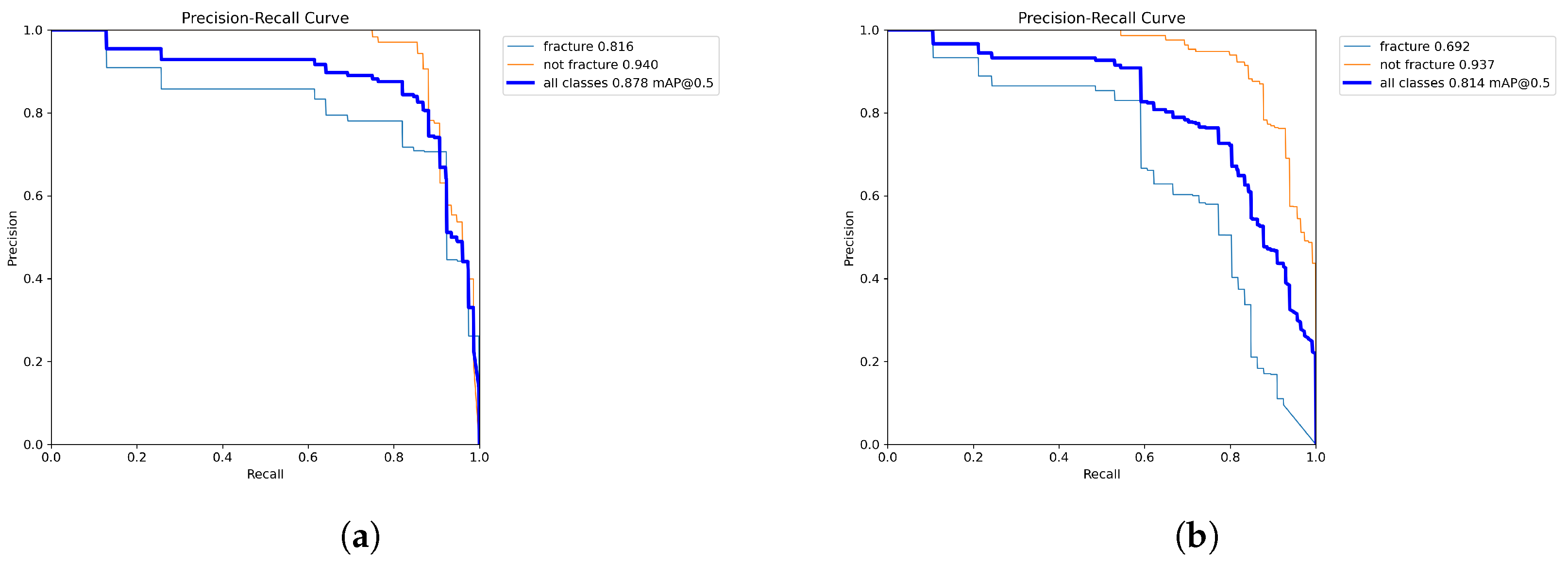
Figure 4.
Example of correct classifications of radiograph photographs: (a) Fracture detected on radiograph photo. (b) Non-fracture detected on radiograph photo.
Figure 4.
Example of correct classifications of radiograph photographs: (a) Fracture detected on radiograph photo. (b) Non-fracture detected on radiograph photo.

Figure 5.
Example of prediciton inconsistency at various angles: (a) Fracture detected on radiograph photo. (b) Non-fracture detected on the same radiograph photo.
Figure 5.
Example of prediciton inconsistency at various angles: (a) Fracture detected on radiograph photo. (b) Non-fracture detected on the same radiograph photo.
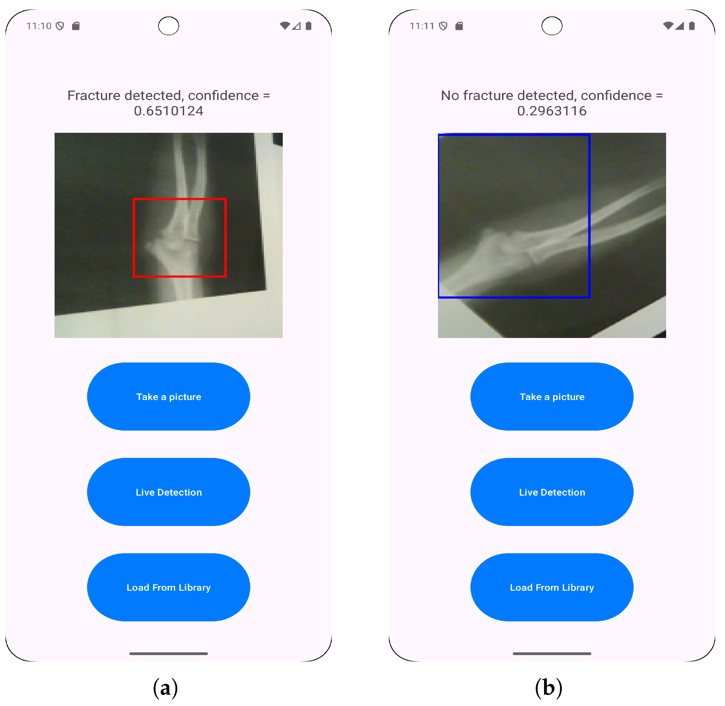
Figure 6.
Examples of successful live predictions: (a) Fracture detected with live detection. (b) Non-fracture detected with live detection.
Figure 6.
Examples of successful live predictions: (a) Fracture detected with live detection. (b) Non-fracture detected with live detection.

Figure 7.
Example showing live detection inconsistency in the same lighting conditions and viewed from the same angle. This was counted as a false negative for the class in the image.
Figure 7.
Example showing live detection inconsistency in the same lighting conditions and viewed from the same angle. This was counted as a false negative for the class in the image.
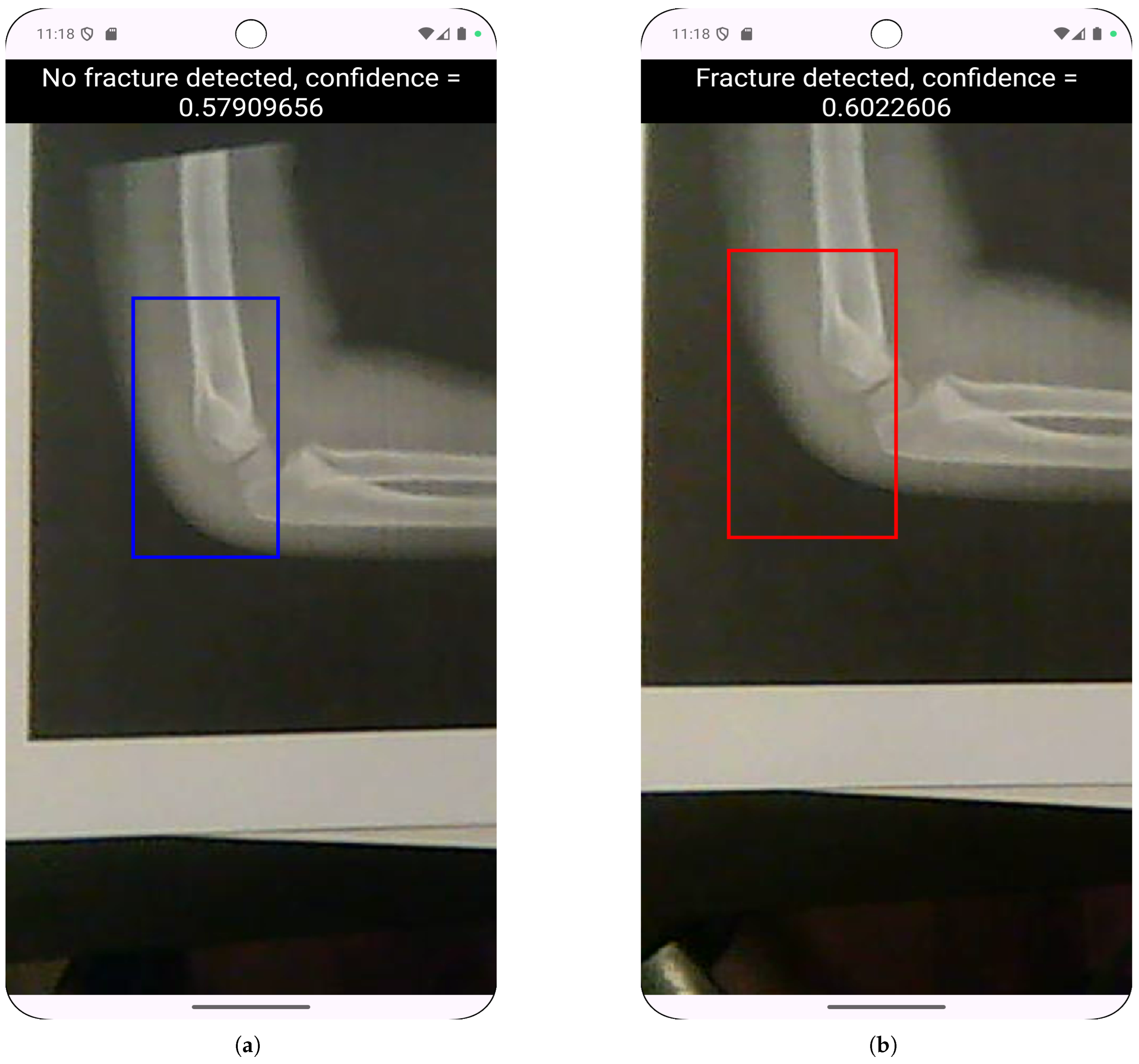
Table 1.
Search parameters for hyperparameter tuning of CNN models.
| Parameters | Values |
|---|---|
| Initial Learning Rate (lr0) | [0.00001 - 0.1] |
| Final Learning Rate (lrf) | [0.01 - 1.0] |
| Batch Size | 16, 32 and 64 |
| Box Loss Weight | [0.02 - 0.2] |
| Classification loss weight | [0.2 - 4.0] |
Table 4.
In-app model performance for Model 1 & 2, for FP16 and FP32 weight quantization.
| Performance Metric | model 1 - FP32 | model 1 - FP16 | model 2 - FP32 | model 2 - FP16 |
|---|---|---|---|---|
| Average F1 Score | 0.927 | 0.927 | 0.913 | 0.913 |
| Average Accuracy | 0.934 | 0.934 | 0.922 | 0.922 |
| Average Bounding Box IoU | 0.699 | 0.699 | 0.683 | 0.683 |
| Average mAP@50 | 0.693 | 0.704 | 0.65 | 0.65 |
| Average mAP@50-95 | 0.342 | 0.343 | 0.305 | 0.305 |
| Average Confidence | 0.698 | 0.698 | 0.676 | 0.676 |
Table 6.
Resource usage for journey 1.
| Device | Average RAM Usage (GB) | Average CPU Usage (%) |
|---|---|---|
| Pixel 3 | 0.173 | 3.492 |
| Pixel 8 Pro | 0.168 | 3.621 |
Table 7.
Resource usage for journey 2.
| Device | Average RAM Usage (GB) | Average CPU Usage (%) |
|---|---|---|
| Pixel 3 | 0.253 | 23.55 |
| Pixel 8 Pro | 0.29 | 24.931 |
Table 9.
Summary of results for live model inference. Further results can be found in tables A.5-A.8 in the appendix.
Table 9.
Summary of results for live model inference. Further results can be found in tables A.5-A.8 in the appendix.
| Model | Lighting | Average Precision | Average Recall | Average F1 Score |
|---|---|---|---|---|
| 80/10/10 FP32 | Daylight | 0.479 | 0.433 | 0.423 |
| 80/10/10 FP32 | Artificial | 0.457 | 0.4 | 0.396 |
| 80/10/10 FP16 | Daylight | 0.295 | 0.3 | 0.288 |
| 80/10/10 FP16 | Artificial | 0.5 | 0.417 | 0.431 |
Disclaimer/Publisher’s Note: The statements, opinions and data contained in all publications are solely those of the individual author(s) and contributor(s) and not of MDPI and/or the editor(s). MDPI and/or the editor(s) disclaim responsibility for any injury to people or property resulting from any ideas, methods, instructions or products referred to in the content. |
© 2025 by the authors. Licensee MDPI, Basel, Switzerland. This article is an open access article distributed under the terms and conditions of the Creative Commons Attribution (CC BY) license (http://creativecommons.org/licenses/by/4.0/).
Copyright: This open access article is published under a Creative Commons CC BY 4.0 license, which permit the free download, distribution, and reuse, provided that the author and preprint are cited in any reuse.


