
Submitted:
11 November 2025
Posted:
12 November 2025
You are already at the latest version
Abstract
The number of industrial processes where smart devices have been employed rises every day; these devices can be found performing tasks related to the automation, digitization, or optimization of the process. Generally for these tasks the devices need to communicate with each other and with a central unit monitored by humans; which is where Industrial Internet of Things IIoT comes to place, allowing to build a network between the devices. Communication might be enough for monitoring purposes but the optimization and automation of the process are yet to be addressed. In this study we explore the Artificial Neural Twin (ANT) as a distributed process optimization tool in combination with Orthogonal Weight Modification (OWM) a continual Learning (CL) method used to augment self-operating devices with the capacity of learning new tasks autonomously. Some of these devices (i.e. microcontrollers used for machine-vision sensors) lack the hardware capacity to run a CL algorithm, which motivated this study, towards comparing Fisher matrix, NEig-OWM, LoRA as large-matrix approximations, towards the complexity reduction of the matrix operations. We found Fisher matrix as the least expensive solution with a negligible reduction on model's performance after CL which would be the most viable solution for large AI-models, while NEig-OWM is optimal for smaller models that require less hardware resources but more control over the CL algorithm.
Keywords:
Internet of Things
; mobile edge computing
; distributed learning
; continual learning
; artificial neural twin
; orthogonal weight modification
1. Introduction
The insertion of smart sensors and intelligent machines on industrial processes is a widely spread practice nowadays; Industrial Internet of Things (IIoT) focuses on connecting these devices with optimization and process automation purposes [1]. To that end, smart devices need to be capable of collecting, processing and transmitting information from the environment to the network, where it is further processed and then translated into feedback by a server device that transmits back to the end devices of the network [2].
The Artificial Neural Twin (ANT) enhances IIoT devices by enabling decentralized model predictive control setups. It integrates the principles of differentiable data fusion (for distributed data collection) and backpropagation (for distributed feedback) to support optimization and process digitalization [3]. Effective processing of information gathered from both the environment and the network requires dedicated computational units within IIoT devices, typically Artificial Intelligence (AI) models such as object detection systems, trained to execute specific tasks.
Training these models is generally time and data intensive, which makes them a pain point for dynamic processes where the tasks are constantly evolving [4]. Moreover, training a model for a new task leads to the model no longer being able to perform the former task, phenomenon known as catastrophic forgetting [5]. In the field of continual learning (CL), many techniques have been developed for models to learn new tasks while avoiding forgetting, these technique can be used in combination with the ANT as their source of training stimuli. However, within the ANT network, access to the loss function is restricted and therefore, gradient-based-CL methods must be selected, here for example, Orthogonal Weight Modification (OWM), a method that prevents models from forgetting by building a matrix,
that projects training gradients in orthogonal direction to the space formed by the gradients used to learn former tasks (original tasks knowledge space) [6].
The problem of applying OWM in IIoT AI models, lies on storing matrix formed by the gradients produced while learning previous tasks, and processing it to build the projector . , where in a per-layer implementation of OWM, n refers to the length of a corresponding model-layer and m to the number of training samples; intuitively we see that for large layers this implementation becomes infeasible, specially within the capabilities of an end device.
As mentioned, distributed systems consist of several such devices communicating with each other as part of a process. In this study we simulated a small example process, emulating the complexity of an industrial sorting facility, focusing mainly on a vision AI-sensor powered by an object detection model (VGG11), which detects several types of objects on a conveyor belt and calculates the corresponding mass-flow. Afterwards, we mimic the insertion of a previously unseen object, which constitutes the new task to be learned through CL.
The mentioned sensor is an example of Mobile Edge Computing (MEC), which classically has lower latency and energy consumption compared to centralized server IIoT, however, it experiences computational, and memory constraints [7]. Considering these limitations, our goal is to investigate the impact on CL performance and computational complexity of three different representations of matrix : Fisher Information matrix, Low-Rank Approximation (LoRA), and Null Space Eigenface (NEig-OWM), to determine suitable options to implement OWM on those devices.
2. Materials and Methods
Throughout this section we describe the algorithms and tools used to build the experimental setup required for the proper assessment of the tested approaches. We discuss case-specific metrics, and at last, we describe the pipeline for the test cases.
2.1. Artificial Neural Twin (ANT)
The ANT augments the functionality of IIoT network by providing a platform for distributed-process optimization. It’s core idea is to represent processes as neural networks (NN), where machines correspond to the neurons and their parameters to the network weights.
In the ANT like in a NN, during forward pass, all machines communicate their state through the network as shown in Figure 1. Then, they reach a consensus between network-received- and the internal- information of the process stage (ANT-node) through data fusion, to update their state , and forward propagate it on the network. This allows to assess the state at any process stage which is important for quality control assessments, and the evaluation of a global loss function at the exit. The generated loss gradients trigger the backpropagation period, that occurs through the process and time; propagating gradients to each machine involved in the process, and inside them, from future time steps till the present, which allows the optimization of current-machine parameters.
The ANT is able to receive process quality control measurements from the user [3], this means that at any stage, production recordings can be performed and introduced to the digital process. Afterwards, this data is contrasted with the state estimate for the respective ANT-node, then gradients are calculated, and accordingly backpropagated to be used as training stimuli for CL. Another source for this stimuli is generated during data fusion, where as above-mentioned every ANT-node reaches a consensus of its state, process in which data fusion residuals are produced which can be used by AI models to learn new tasks. These sources of training stimuli make the ANT a great ally for implementing CL on industrial process chains.
2.2. Stability-Plasticity Trade-Off
The main properties of a CL technique are the model’s stability and plasticity while learning new tasks. Stability reflects the model’s capacity to retain previous knowledge, while plasticity refers to the capacity to acquire new. A highly stable approach will generate a model that retains knowledge well but that hardly learns, and vice versa for a highly plastic approach. This relation is known as the stability-plasticity trade-off [9].
Stability can be evaluated in terms of the Forgetting Measure (FM) [10], which relates model’s past and current performances,
where refers to the model’s maximum performance (fort this study we used F1-score as a metric) on task j calculated after learning task i, likewise is calculated after learning the new task k. Then, the forgetting at k-th task,
from where the stability is simply calculated as,
The plasticity on the other hand refers to the model’s capacity to learn new tasks, this is evaluated in terms of its convergence speed on the new task,
where corresponds to the performance right after convergence, and refers to the epochs necessary to reach convergence.
These two properties define the learning capacity of a model under specific CL conditions. Intuitively we observe the contradiction between them and therefore it’s key to reach a reasonable trade-off [11] where the model is capable of acquiring new knowledge without considerable performance compromises.
2.3. Fisher Information Matrix
In supervised learning, training AI models means to find a set of parameters () for which given the input set (x) the model is capable of closely approximating the output (y). In other words, given the training set S(x,y), the goal is to minimize the objective function,
where is a loss function that measures the differences between the model’s prediction z and the target y. This applies for any loss function, for example the cross-entropy loss . Differentiating the loss w.r.t. , we obtain the respective gradients [12].
The Fisher matrix of the model’s learned distribution w.r.t. is,
since , where does not depend on , then, , where the input x comes from an independent target distribution, with as its density function, then the Fisher matrix can be expressed,
which represents the Fisher information matrix formed by the loss gradients produced while learning the model’s parameter distribution , using cross-entropy loss [13] This means that the Fisher matrix is the hessian matrix of the cross-entropy loss [14].
Regularization-based CL approaches like Elastic Weight Consolidation (EWC), used the diagonal of the Fisher matrix to penalize the learning of new tasks [15], in this article we will use the same diagonal to build the projector matrix for OWM.
2.4. Low-Rank Approximation (LoRA)
Due to computational complexity, conventional machine learning methods can become inapplicable when dealing with large matrices. Traditionally, data reduction techniques are used to mitigate this issue, which should retain most of the intrinsic information of the original data. Low rank approximation achieves this by decomposing the original matrix into two lower rank (rank-k) matrices [16],
The optimal k for LoRA is typically obtained by minimizing the Frobenius norm between and its approximation , then , where the Forbenius norm, , of a matrix is given by , then can be formulated as a Singular Value Decomposition (SVD) of . Since the SVD of is , where and are orthogonal, , and . Then for , the minimum is achieved with , where , and and are the matrices formed by the first k columns of and respectively [17].
2.5. Null Space Eigenface (NEig-OWM)
Many approaches have been developed towards balancing the stability-plasticity trade-off. Architecture-based-approach researchers concluded that deeper models show better plasticity and wider models better stability [18]. Normalization based approaches introduce normalization layers with different strengths to maintain both high stability and plasticity [9]. Optimization-based techniques focus on enhancing the parameter updating rules, by either introducing regularization terms or modifying the gradients applied to the model. OWM belongs to the second category, since it influences the parameter updating . NEig-OWM however, updates the parameters while targeting directly the stability-plasticity trade-off [19], including in its projector a specific term for the respective property,
where refers to the null space formed by the eigen vectors whose corresponding eigen values are equal to zero , refers to the orthogonal projector matrix formed by the eigen vectors whose eigen values are different from zero, and is a hyper-parameter that regulates new learning. increases models stability by projecting new knowledge orthogonally to previous, and the second term enhances plasticity by favoring the learning on previously unused areas of the model.
2.6. Experimental Setup
As mentioned, for our experiments we simulated a section of a bulk material recycling process, using the physics engine of Unity game development framework [20]. This controlled environment provides us with a material stream that emulates the complexity of a real material sorting task. Inside the simulated process, we begin with a machine (“siever”) that sorts materials by size (Small, Medium, Large), on each outlet we placed conveyor belts that emulate the delay between sorting machines, and after each of them we placed magnetic sorters, which sort materials as metallic and non-metallic as per the flow diagram in Figure 2.
Within our simulation each device is independent and insulated from the information network, then the ANT allows to convert this into a machine learning distributed system, providing a platform for all devices to exchange information, for the process to be optimized, and the models to be trained though CL.
The AI-sensor subject of this study is set above the middle conveyor belt, as highlighted in the diagram, which is a location reached by the full set of objects involved in the process. Figure 3 depicts the mentioned set, from where we initially removed the Cans (a) that later will be used as a continual learning task.
Within the simulation, we configure the sensor’s area of vision such that 1080x512 pixel images correspond to one second mass-flow of the process. This allows calculation of mass-flow either per-second or higher resolutions. Table 1 shows the material distribution throughout the different datasets collected using this data configuration.
2.7. Test Cases
Even though continual learning is usually performed online (During process operation), the initial training (Training dataset as per Table 1) of the AI model is typically done offline. During this period we collect the training loss gradients, such that at the end for each model layer we obtain a matrix where the rows are given by the number of layer parameters, and the columns by the number of training samples. These matrices represent the original task’s knowledge space which should be preserved during CL [6].
We extract all representations from the respective of each layer. Since we used cross entropy loss for the initial training, Fisher matrix as per Equation 8 will correspond to multiplied by its transpose, from where we will extract and store only the diagonal to build the OWM projector. For LoRA approximation of we apply SVD, then extract and store the lower rank and as explained in Section 2.4. In NEig-OWM we divide matrix into two matrices as per Equation 10, where we extract the eigen vectors and eigen values, separating the null and non-null space, and store their corresponding matrices.
The focus of our investigation is to evaluate alternative representations for matrix that better fit hardware and networking constraints, therefore, the model, dataset, loss function, optimizer, and OWM as CL method remained constant throughout our experiments. Meanwhile, we tuned the parameterization (Validation dataset as per Table 1) of the representation approaches to better approximate the original .
Algorithm 1 summarizes the CL training process (CL dataset as per Table 1) used in our research. Here each image is used for training only once, thereafter, they can be used as a measurement for convergence speed. This algorithm shows as well our implementation of OWM in a per-layer configuration, which reduces the memory required to project a gradient vector.
| Algorithm 1: CL Training Loop |
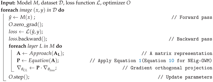 |
Here we apply the approach in turn to extract the specific matrix representation of and instead of materializing in memory the larger matrix P, we multiply the gradient by each term of Equation 1, reducing the load in memory from to , where and represent the terms in the projector’s equation, and . This exempt us from storing matrix in memory, but instead, smaller matrix . Afterwards, as typically the modified gradients were used to update model’s parameters.
As per Algorithm 1 we use OWM to learn the new task (Detecting and classifying Can objects) recording test performance metrics (CL-Testing dataset as per Table 1) to determine the efficiency of the different approaches during CL. We included the full matrix and the pure Stochastic Gradient Descent (SGD) as top and bottom lines of the benchmark used to assess the performance of the tested approaches.
The result section will summarize the scores of our experiments on the described as well as standard metrics, such as: F1-score, Precision, recall, and individual metrics drawn from a confusion matrix.
3. Results
As explained, the AI sensor is originally trained to detect four objects (Bottle, Coffee cup, paper ball, paper roll) which we refer to as the original task, Figure 4 denotes its performance (F1 score of 86.70%) after the mentioned training, shown by the big dot (Testing dataset as per Table 1) set at position zero CL training images.
For every approach, we begin the CL with an evaluation (F1 score 72.82%) on CL test data, this decrement on performance compare to the original task is produced by miss-classifications on the new task. Then, we train the model on gradients generated by one image at the time with evaluations on the test data set every fifteen training images.
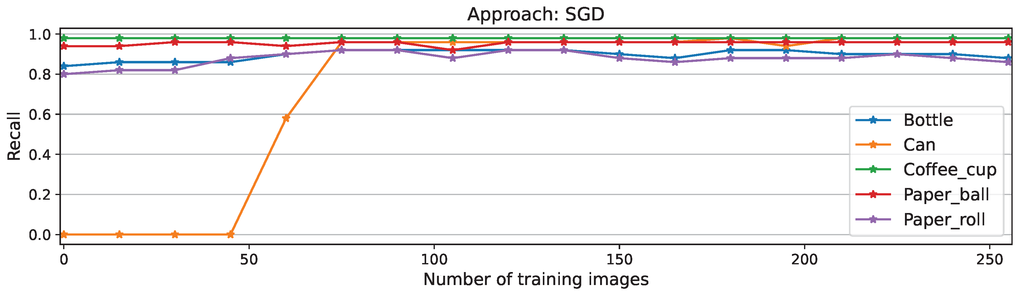
Among the approaches, as expected the best performance is recorded while using the full matrix, which manages to learn the new task after only 60 training images, reaching 85.17% as its maximum performance, followed by a minimal forgetting phase to finalize the experiment at 82,64%. Similar behavior was recorded by NEig-OWM approach with maximum and final F1 scores of 84,24% and 81.45% respectively. Fisher matrix comes third learning the new task after 105 images, with its maximum at 84,41% and a final performance of 81.45% exactly as NEig-OWM. LoRA and SGD show catastrophic forgetting since the beginning of CL, as shown by the drops in their curves; this is even more clearly visible on their corresponding precision curves depicted in Figure A5 and Figure A7, respectively, where the per-object performance is shown. Afterwards, they learned the new task showing an increment on their overall performance which is still comparatively low finishing the experiment both at an F1 score of 73.84%.
The described results are confirmed by the confusion matrices in Figure 5, were once again full matrix’s performance is the highest while LoRA’s and SGD’s are the lowest. On the upper left corner, we have the confusion matrix of the original model (before CL) on the new task; where the decrement on performance due to false positive classifications is clearly visible. This is no longer the case after finishing the CL (All other confusion matrices), where despite the remaining cases of miss classification between can and coffee cup classes, it is visible that the model can perform the new task properly. The unavoidable forgetting due to CL is present in all classes as minimal increment on the false positive scores; and as before LoRA and SGD have the highest rates, showing percentages higher than 15% on the false positive classifications of almost every class.
In the comparison of memory and complexity requirements in Figure 6 (right), the minimum is at SGD, which represents no implementation of CL approach. Therefore, no memory nor additional computations are required, followed by Fisher matrix where the storage of only the matrix diagonal gives a marked advantage in memory requirement compared to others, from the diagonal we approximated which translates in equal complexity as when using full matrix, which is also the case for LoRA. Since NEig-OWM divides matrix in two and generates a projector per each section, this translates into same storage requirements as per full , but double the computational operations.
For stability-plasticity trade-off in Figure 6 (left), the average stability through classes shows similar behavior on full , Fisher matrix, and NEig-OWM, while a lower score is recorded on LoRA and SGD due to higher forgetting. Meanwhile, plasticity is calculated exclusively on the new task. High plasticity is shown by LoRA, SGD and NEig-OWM, where the former two are highly plastic due to lower stability, while NEig-OWM remains high on both properties thanks to its mentioned characteristics that address this trade-off specifically. The higher stability using the full matrix is contrasted by lower plasticity; this effect is even greater while using Fisher matrix where the plasticity drops to 40%.
The low memory requirements and complexity, plus its high stability despite its lower plasticity makes Fisher matrix the minimum and best performing approach. Therefore, in this last section we will focus mostly on its results.
Per-class precision for Fisher matrix approach is shown in Figure 7, here the learning process of the new task is clearly visible, with an initial peak on performance at 90 training images due to model’s double detection (cans labeled as coffee cups and cans simultaneously), which was later overcome converging at 56.72% precision on the new task, which was not the highest score, but the most steady convergence compared to equivalent plots for other approaches displayed in Figure A1, Figure A3, Figure A5, and Figure A7.
The stability of the approach is displayed here by the nearly constant scores of known classes; except for the class coffee cup, which initially included falsely classified cans. This issue is clarified on the recall plots on Figure 8, where false positives have no influence and therefore all-other-class scores remain constant while the new-class score improves. This plot shows as well the longer time before convergence on this approach compared to full , NEig-OWM, LoRA, and SGD depicted on Figure A2, Figure A4, Figure A6, and Figure A8 respectively.
4. Discussion
The LoRA approach did not perform much better than applying plane SGD, which we understand is due to the highly minimized rank while approximating , which predicated on loosing parameters important for defining the original task knowledge space. Given that our objective is to find the least expensive solution, we considered there was no need for further search of a higher rank approximation. Moreover, the diagonal of Fisher matrix proven to be a less expensive while effective option. We consider this as the best solution for large models installed on devices with relatively tight hardware constraints; as depicted in Figure 4 and confirmed by its plasticity score in Figure 6, its learning speed is comparatively slow but its end performance matches the highest recorded, with the lowest hardware requirements.
We presented full as a benchmark, however, this is still a viable option for scenarios with medium to large models, where the hardware is not considerably restrictive and a faster learning speed is required. NEig-OWM is the approach with the highest hardware demands which makes it applicable for situations with no restrictions; or when hardware constraints are overcome by implementing small models, which however present bigger parameter overlap between tasks. Here the approach’s direct regard for the stability-plasticity trade-off allows for greater segregation of the non-overlapping areas of the model which translates in greater control over the forgetting while learning new tasks.
Our future research involves: CL on a vision sensor, powered by a large object detection model with a Fisher matrix representation of matrix ; and the implementation of NEig-OWM on a small machine model (i.e. the input/output prediction model of a magnetic sorter). We will insert both models in the ANT network so that we can analyze the performance of CL using QC-gradients and DF-residuals as training stimuli.
Abbreviations
The following abbreviations are used in this manuscript:
| ANT | Artificial Neural Twin |
| AI | Artificial Intelligence |
| CL | Continual Learning |
| DF | Data Fusion |
| EWC | Elastic Weight Consolidation |
| Fl | Flow sensor |
| FM | Forgetting Measure |
| IIoT | Industrial Internet of Things |
| LoRA | Low Rank Approximation |
| MEC | Mobile Edge Computing |
| NN | Neural Network |
| NEig-OWM | Null Eigenface - Orthogonal Weight Modification |
| OWM | Orthogonal Weight Modification |
| QC | Quality Control |
| SGD | Stochastic Gradient Descent |
| SVD | Singular Value Decomposition |
| VGG11 | Visual Geometry Group 11 |
Appendix A
Figure A1.
Per-class precision scores for full matrix approach
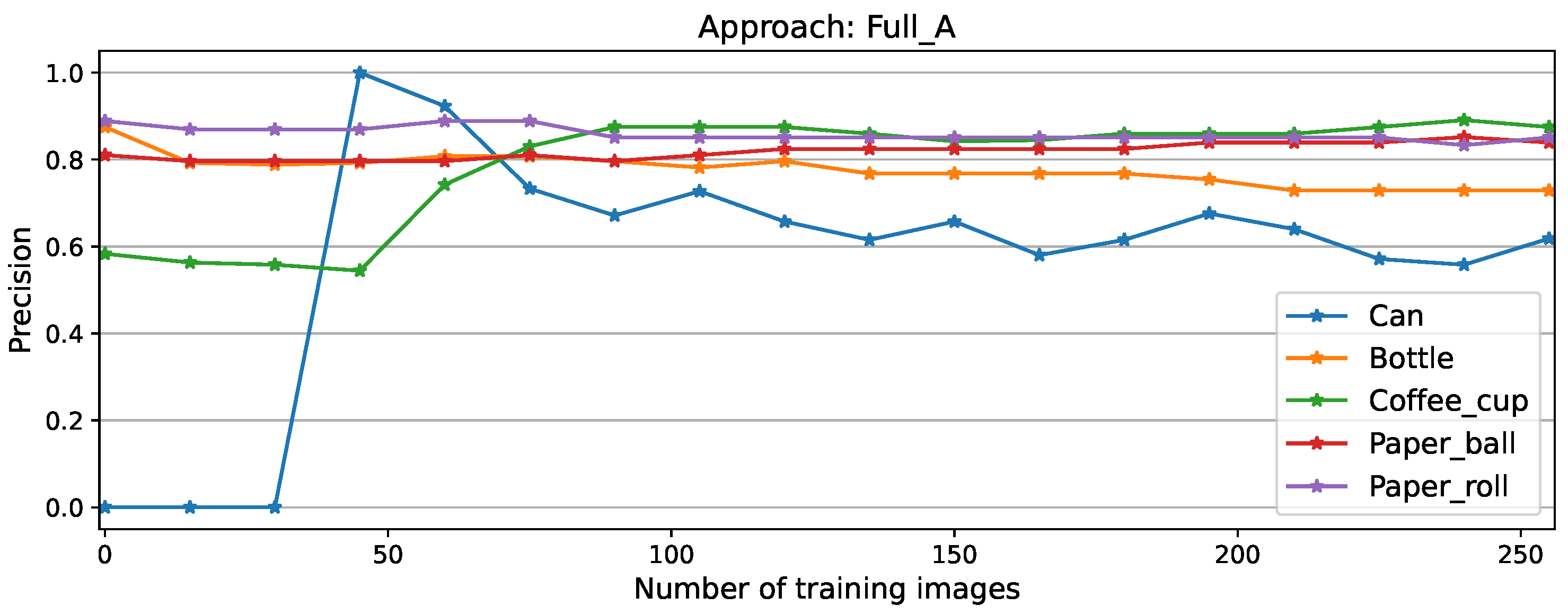
Figure A2.
Per-class recall scores for full matrix approach
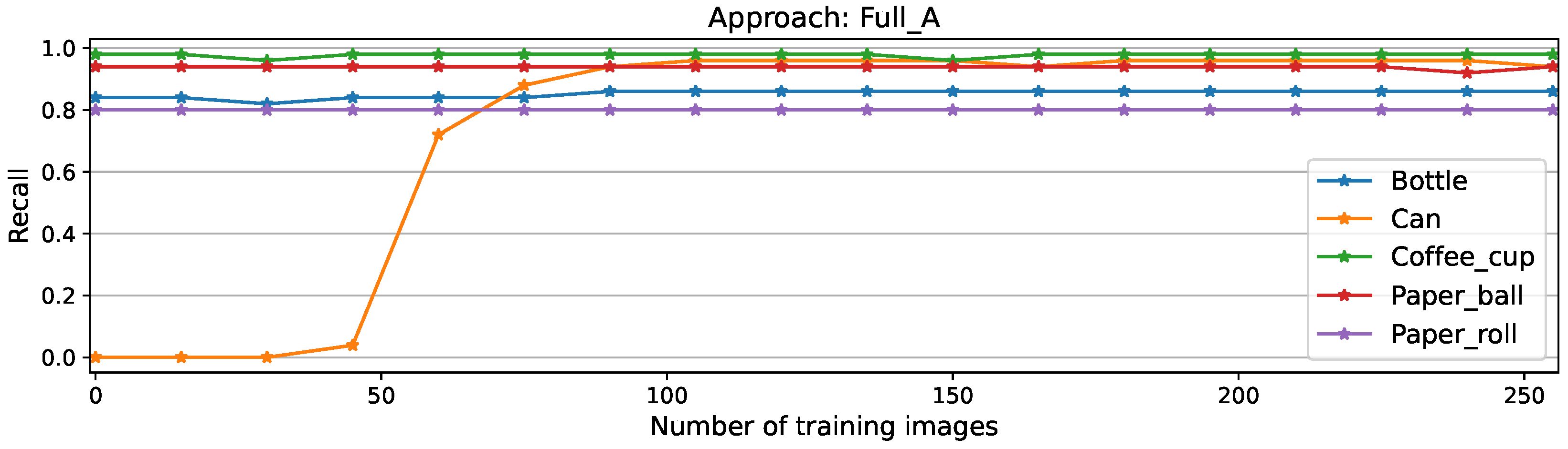
Figure A3.
Per-class precision scores for NEig-OWM approach
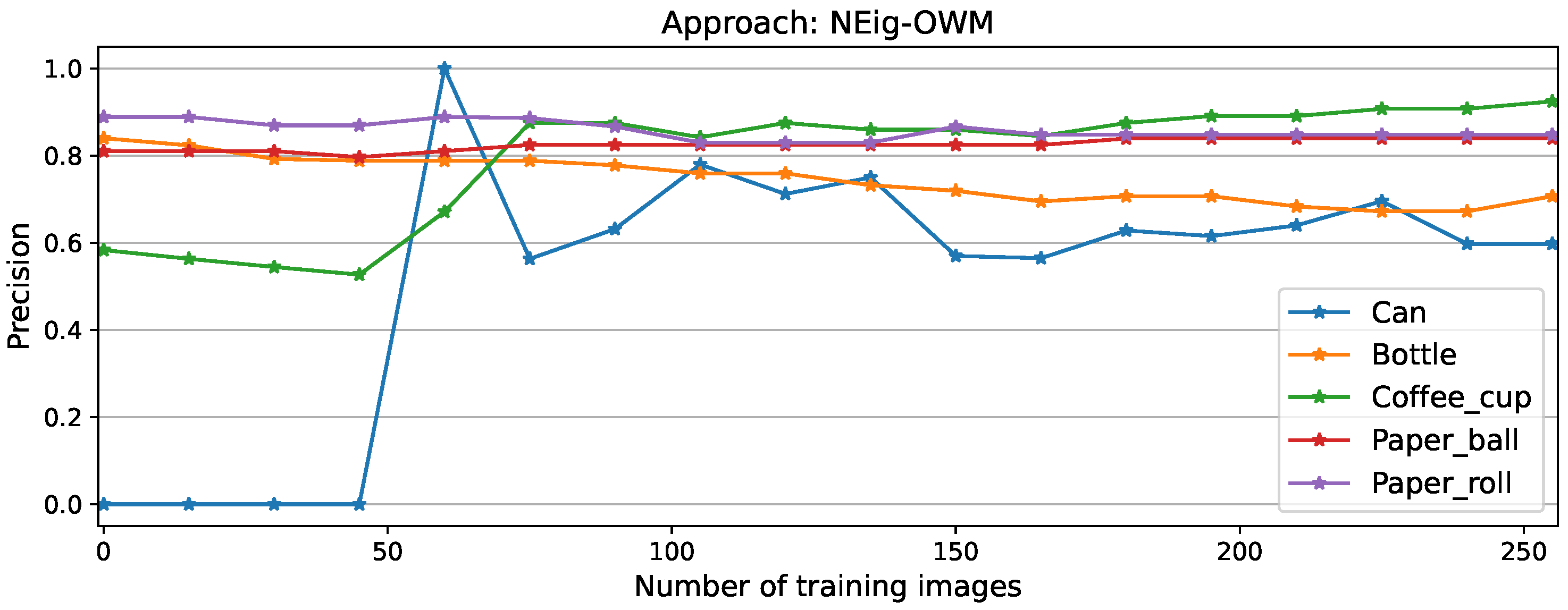
Figure A4.
Per-class recall scores for NEig-OWM approach
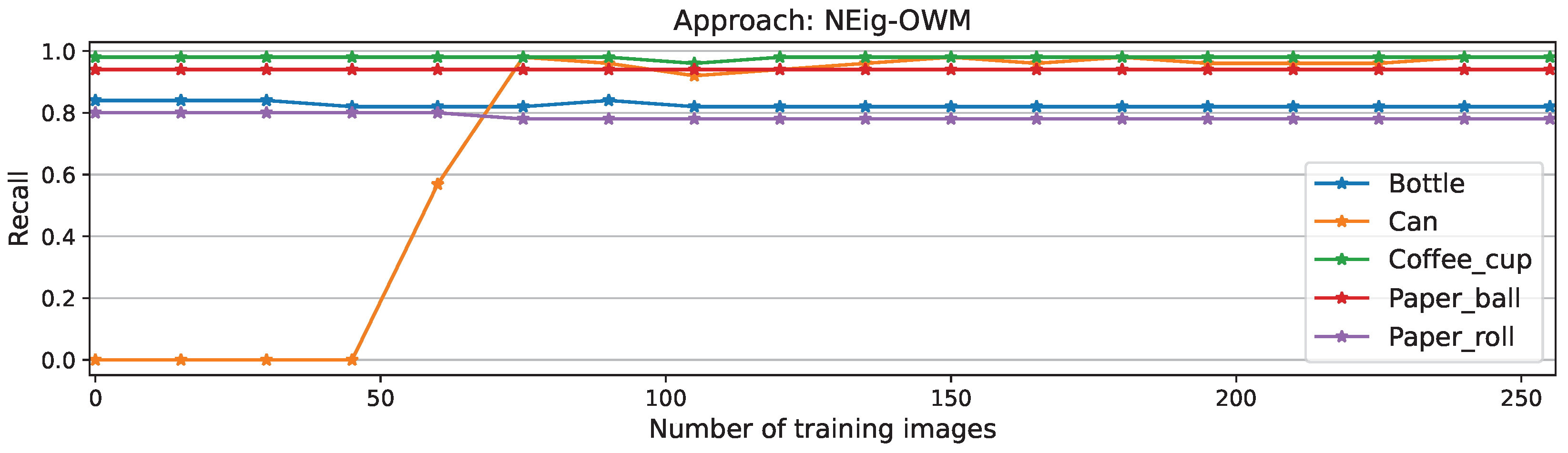
Figure A5.
Per-class precision scores for LoRA approach
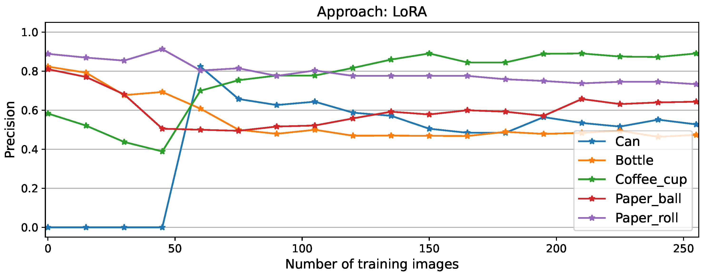
Figure A6.
Per-class recall scores for LoRA approach
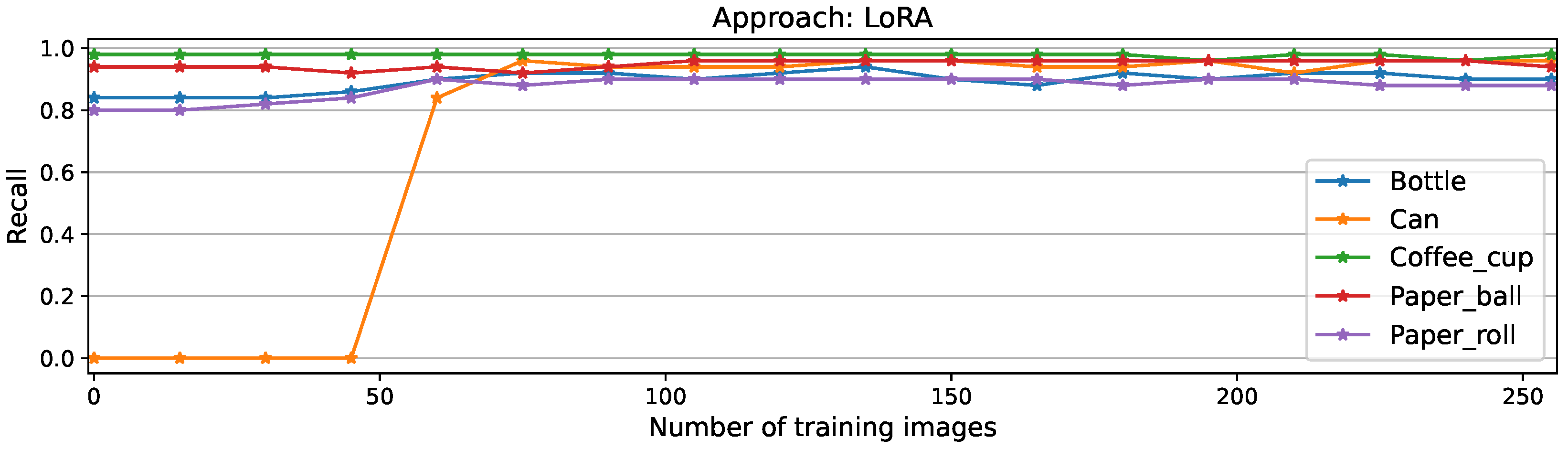
Figure A7.
Per-class precision scores for SGD approach
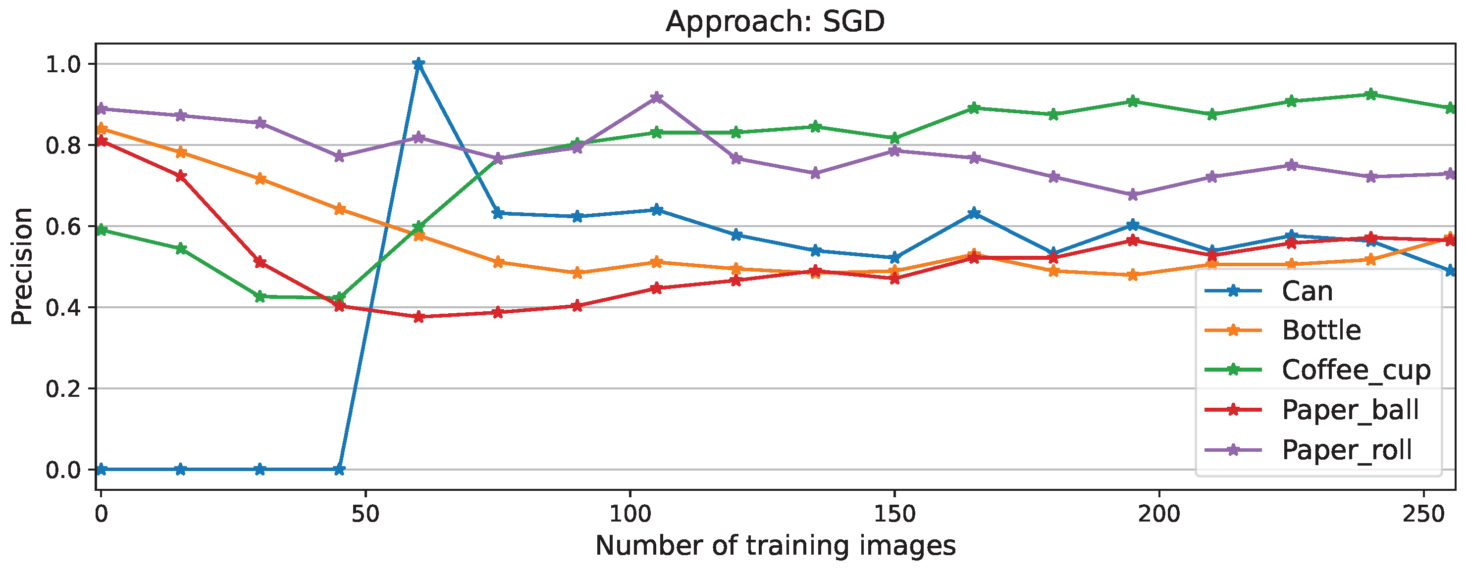
Figure A8.
Per-class recall scores for SGD approach
References
- Serror, M.; Hack, S.; Henze, M.; Schuba, M.; Wehrle, K. Challenges and Opportunities in Securing the Industrial Internet of Things. IEEE Transactions on Industrial Informatics 2021, 17, 2985–2996. [Google Scholar] [CrossRef]
- Sisinni, E.; Saifullah, A.; Han, S.; Jennehag, U.; Gidlund, M. Industrial Internet of Things: Challenges, Opportunities, and Directions. IEEE Transactions on Industrial Informatics 2018, 14, 4724–4734. [Google Scholar] [CrossRef]
- Emmert, J.; Mendez, R.; Dastjerdi, H.M.; Syben, C.; Maier, A. The Artificial Neural Twin — Process optimization and continual learning in distributed process chains. Neural Networks 2024, 180, 106647. [Google Scholar] [CrossRef] [PubMed]
- Basedow, N.; Hadasch, K.; Dawoud, M.; Colloseus, C.; Taha, I.; Aschenbrenner, D. Open Data Sources for Post-Consumer Plastic Sorting: What We Have and What We Still Need. Procedia CIRP 2024, 122, 1042–1047. [Google Scholar] [CrossRef]
- Parisi, G.I.; Kemker, R.; Part, J.L.; Kanan, C.; Wermter, S. Continual lifelong learning with neural networks: A review. Neural Networks 2019, 113, 54–71. [Google Scholar] [CrossRef] [PubMed]
- Guanxiong, Z.; Yang, C.; Bo, C.; Shan, Y. Continual learning of context-dependent processing in neural networks. Nature Machine Intelligence 2019, 1, 364–372. [Google Scholar] [CrossRef]
- Tang, S.; Chen, L.; He, K.; Xia, J.; Fan, L.; Nallanathan, A. Computational Intelligence and Deep Learning for Next-Generation Edge-Enabled Industrial IoT. IEEE Transactions on Network Science and Engineering 2023, 10, 2881–2893. [Google Scholar] [CrossRef]
- Mendez, R.; Maier, A.; Emmert, J. Towards continual learning with the artificial neural twin applied to recycling processes.
- Jung, D.; Lee, D.; Hong, S.; Jang, H.; Bae, H.; Yoon, S. New Insights for the Stability-Plasticity Dilemma in Online Continual Learning. In Proceedings of the The Eleventh International Conference on Learning Representations; 2023. [Google Scholar]
- Verma, T.; Jin, L.; Zhou, J.; Huang, J.; Tan, M.; Choong, B.C.M.; Tan, T.F.; Gao, F.; Xu, X.; Ting, D.S.; et al. Privacy-preserving continual learning methods for medical image classification: a comparative analysis. Frontiers in Medicine 2023, 10, 1227515. [Google Scholar] [CrossRef] [PubMed]
- Wang, L.; Zhang, X.; Su, H.; Zhu, J. T: Comprehensive Survey of Continual Learning, 2024; arXiv:cs.LG/2302.00487. [CrossRef]
- Martens, J. New Insights and Perspectives on the Natural Gradient Method. J. Mach. Learn. Res. 2014, 21, 146–1. [Google Scholar]
- Yang, M.; Xu, D.; Cui, Q.; Wen, Z.; Xu, P. An Efficient Fisher Matrix Approximation Method for Large-Scale Neural Network Optimization. IEEE Transactions on Pattern Analysis and Machine Intelligence 2023, 45, 5391–5403. [Google Scholar] [CrossRef] [PubMed]
- Kong, Y.; Liu, L.; Chen, H.; Kacprzyk, J.; Tao, D. Overcoming Catastrophic Forgetting in Continual Learning by Exploring Eigenvalues of Hessian Matrix. IEEE Transactions on Neural Networks and Learning Systems 2024, 35, 16196–16210. [Google Scholar] [CrossRef] [PubMed]
- Kirkpatrick, J.; Pascanu, R.; Rabinowitz, N.; Veness, J.; Desjardins, G.; Rusu, A.A.; Milan, K.; Quan, J.; Ramalho, T.; Grabska-Barwinska, A.; et al. Overcoming catastrophic forgetting in neural networks. Proceedings of the National Academy of Sciences 2017, 114, 3521–3526. [Google Scholar] [CrossRef] [PubMed]
- Kumar, N.K.; Schneider, J. Literature survey on low rank approximation of matrices. Linear and Multilinear Algebra 2017, 65, 2212–2244. [Google Scholar] [CrossRef]
- Ye, J. Generalized low rank approximations of matrices. In Proceedings of the Proceedings of the Twenty-First International Conference on Machine Learning, New York, NY, USA, 2004. [CrossRef]
- Lu, A.; Yuan, H.; Feng, T.; Sun, Y. Rethinking the Stability-Plasticity Trade-off in Continual Learning from an Architectural Perspective. 2025; arXiv:cs.LG/2506.03951]. [Google Scholar]
- Liao, D.; Liu, J.; Zeng, J.; Xu, S. The continuous learning algorithm with null space and eigenface-based orthogonal weight modification. Expert Systems with Applications 2025, 281, 127468. [Google Scholar] [CrossRef]
- Juliani, A.; Berges, V.P.; Teng, E.; Cohen, A.; Harper, J.; Elion, C.; Goy, C.; Gao, Y.; Henry, H.; Mattar, M.; et al. Unity: A General Platform for Intelligent Agents. 2020; arXiv:cs.LG/1809.02627]. [Google Scholar] [CrossRef]
Figure 1.
ANT forward and backpropagation periods, where refers to the model of ANT-node i, with i; as the input material flow, the output; and the process output. refers to the gradient w.r.t. the ANT-node’s state , gradient with respect to the ANT-node’s parameters , and gradient with respect to model’s parameters . Note: From "Towards continual learning with the artificial neural twin applied to recycling processes", by Mendez et al., 2025 [8]. Licensed under CC BY 4.0.
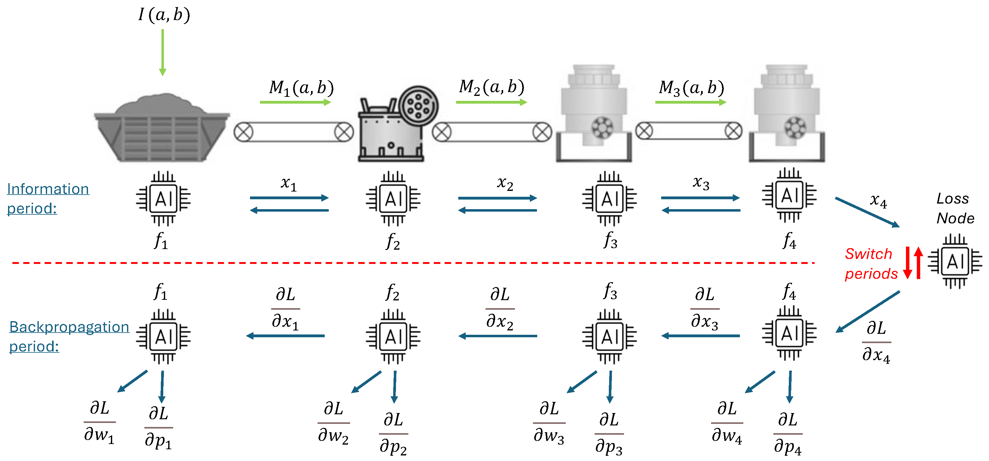
Figure 2.
Flow diagram of sorting process. The input on sieving machine, followed by three conveyor belts, which are each followed by a magnetic sorter, with corresponding Flow sensors (Fl) in several sections of the process. Note: Adapted from "The Artificial Neural Twin—Process optimization and continual learning in distributed process chains" by Emmert et al., 2024 [3]. Licensed under CC BY 4.0.
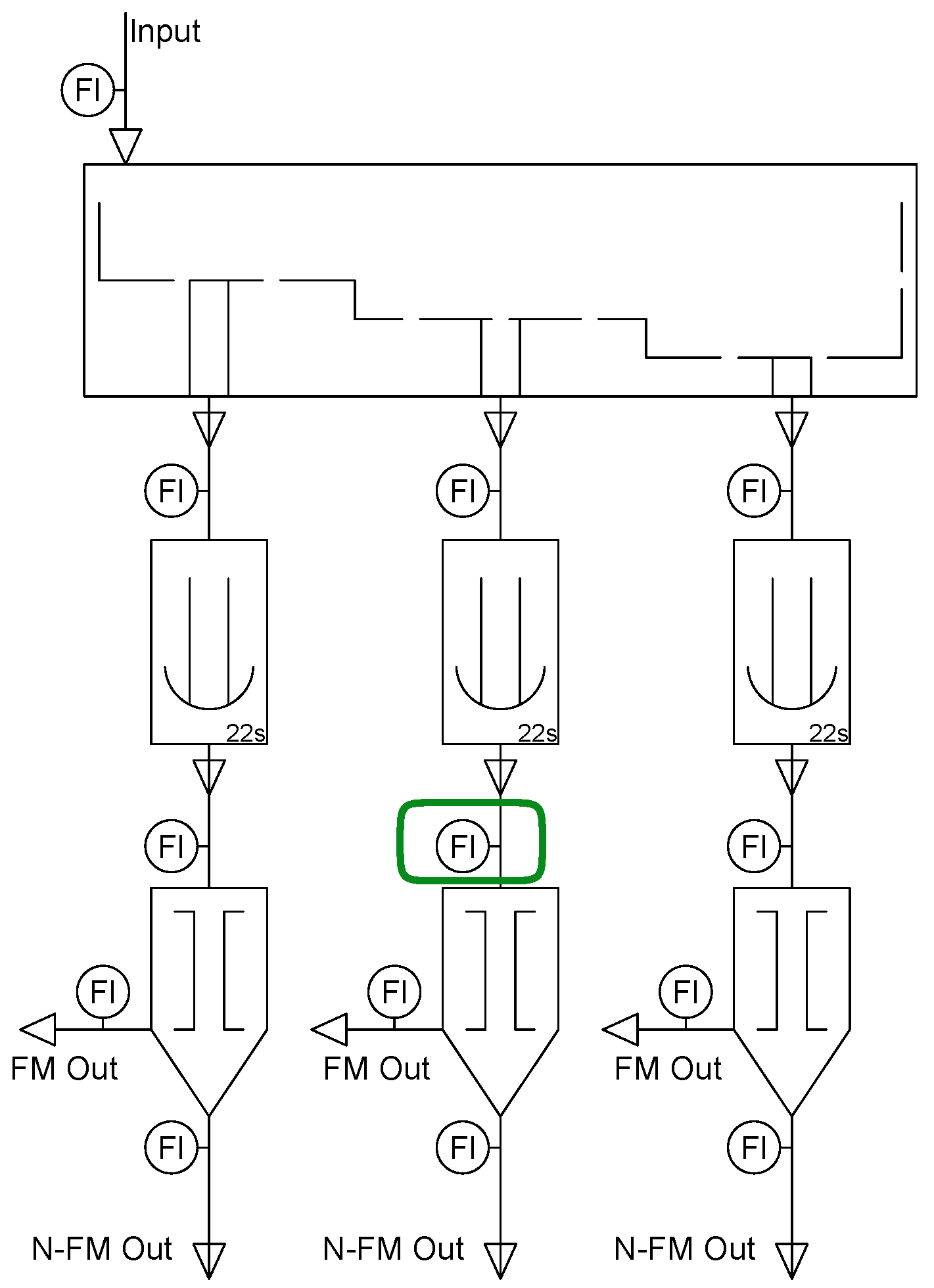
Figure 3.
Objects present in the sorting process a) Can, b) Bottle, c) Coffee cup, d) Paper roll, e) Paper ball
Figure 3.
Objects present in the sorting process a) Can, b) Bottle, c) Coffee cup, d) Paper roll, e) Paper ball
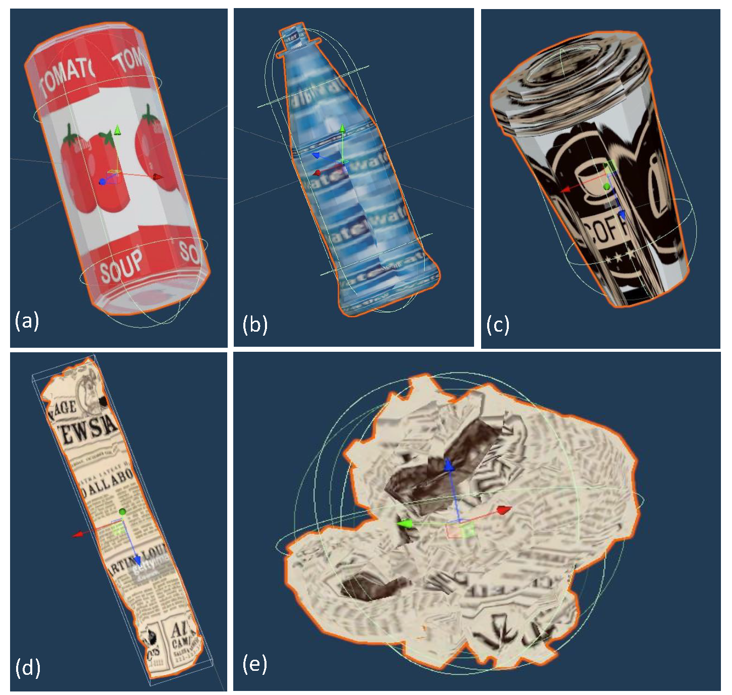
Figure 4.
Model’s F1 score after training for the original task on test data (Initial objects only) denoted by big dot. Model’s F1 scores during CL with all approaches on CL test data (All objects) recorded every fifteen CL training images.
Figure 4.
Model’s F1 score after training for the original task on test data (Initial objects only) denoted by big dot. Model’s F1 scores during CL with all approaches on CL test data (All objects) recorded every fifteen CL training images.
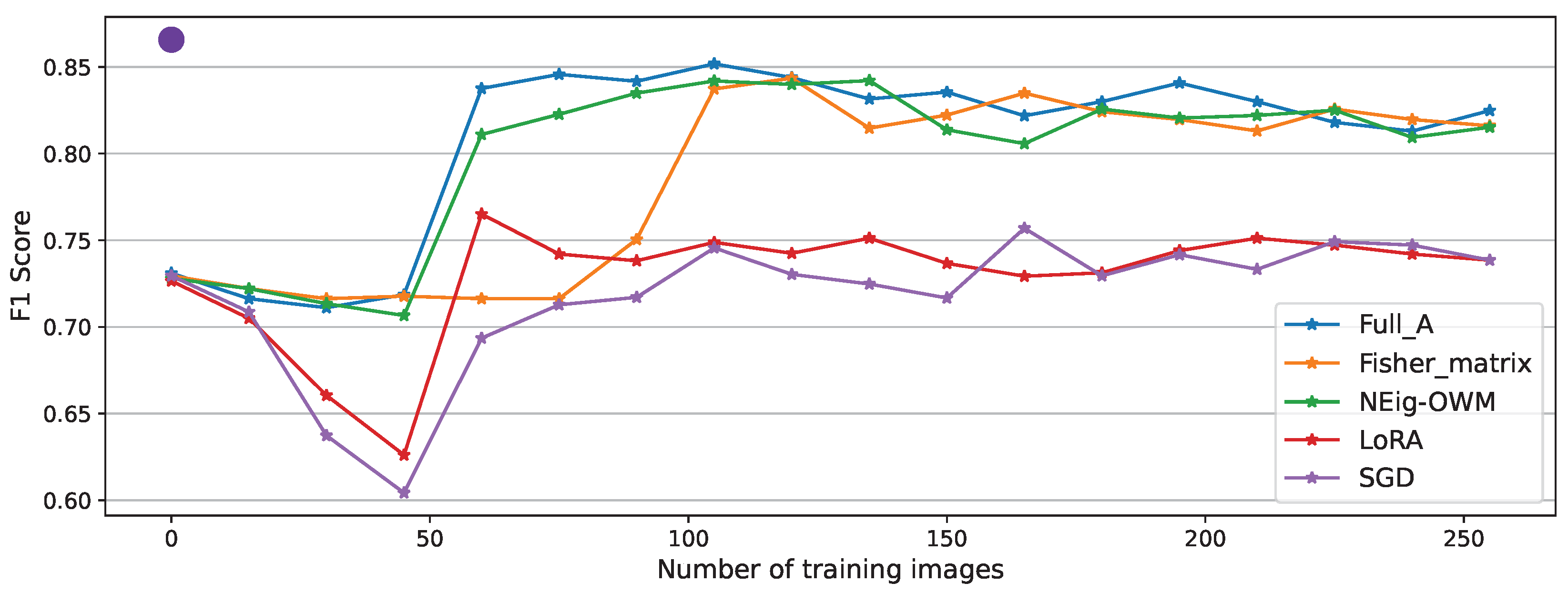
Figure 5.
Confusion matrix of the original model in the original task, followed by confusion matrices after CL with the model trained using every approach and evaluated on CL test data.
Figure 5.
Confusion matrix of the original model in the original task, followed by confusion matrices after CL with the model trained using every approach and evaluated on CL test data.
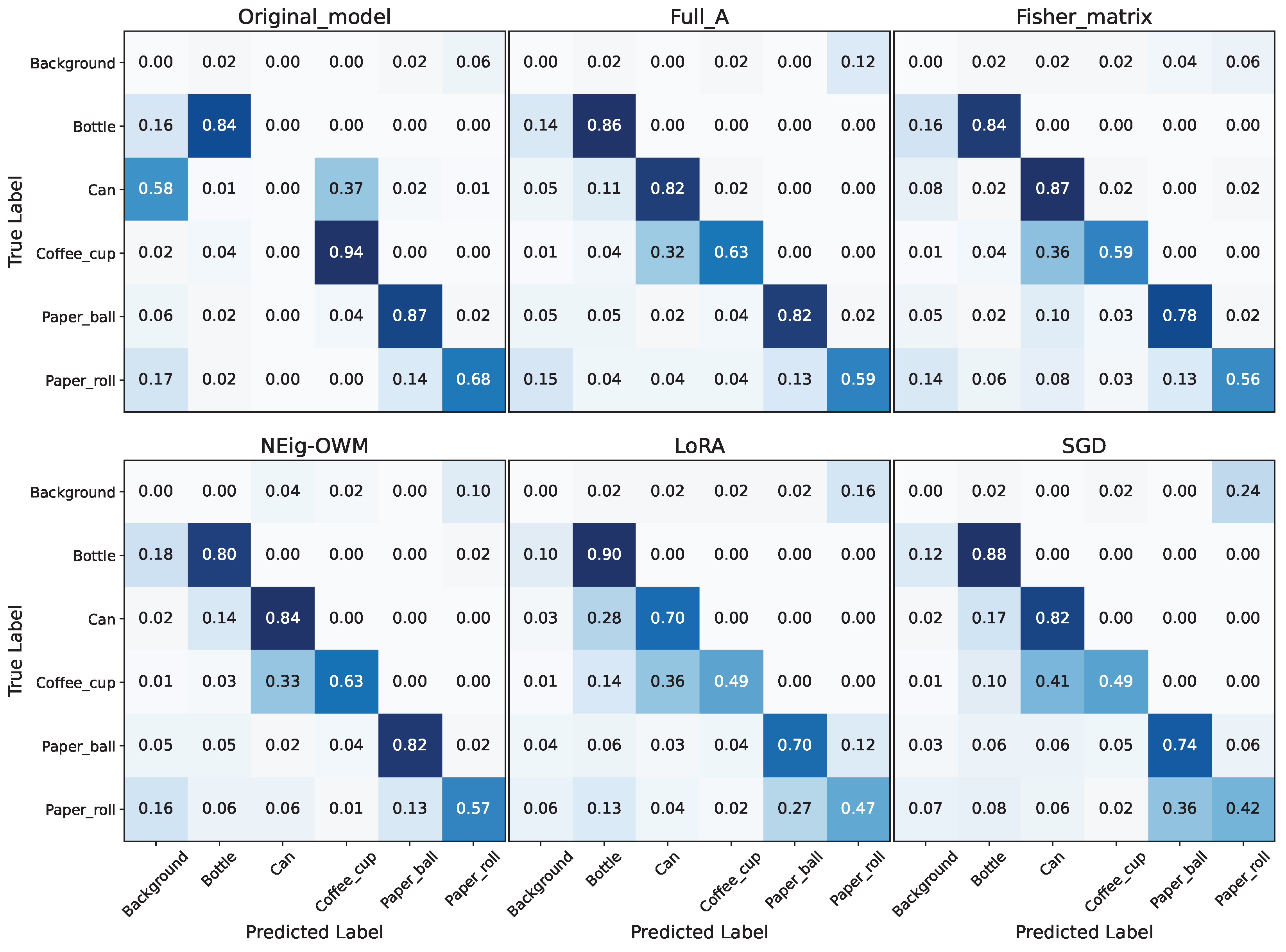
Figure 6.
Approach comparison on stability-plasticity trade-off (left), memory cost and computational complexity (right)
Figure 6.
Approach comparison on stability-plasticity trade-off (left), memory cost and computational complexity (right)
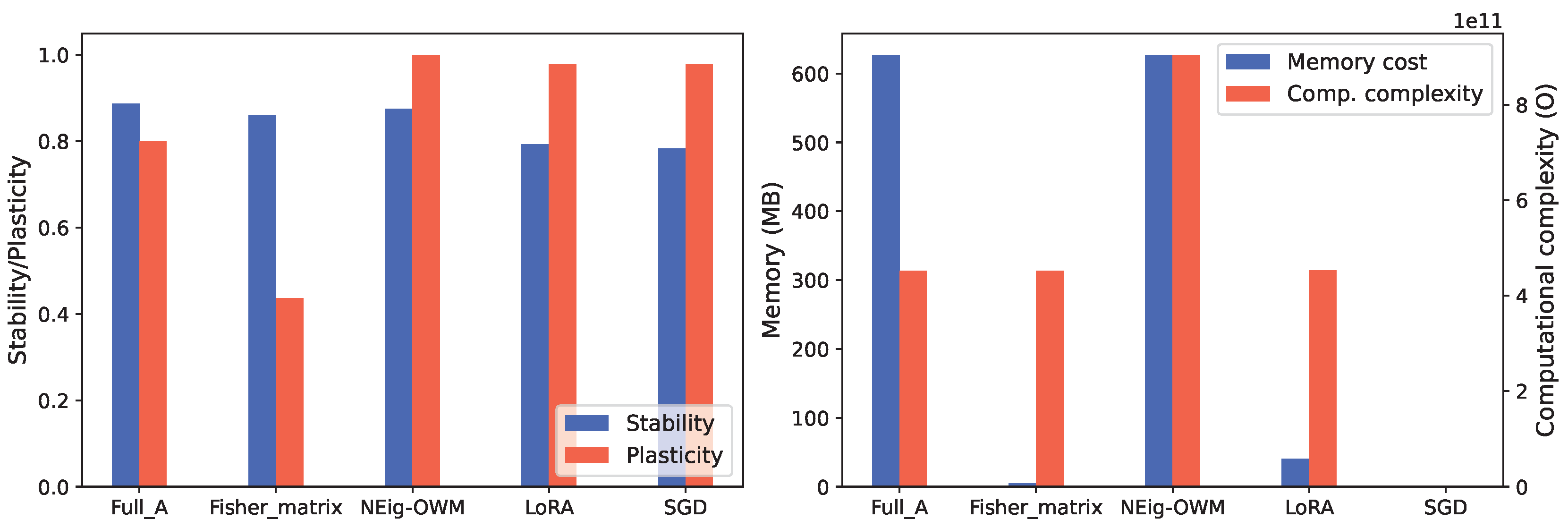
Figure 7.
Per-class precision scores for Fisher matrix approach
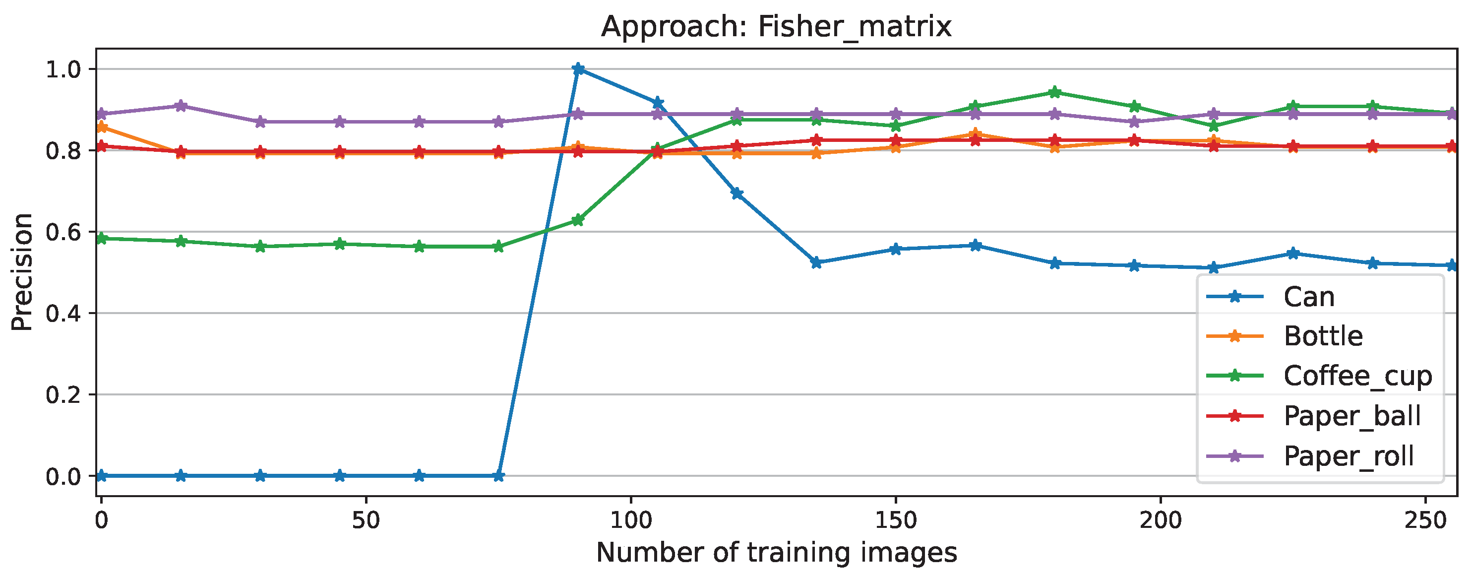
Figure 8.
Per-class recall scores for Fisher matrix approach
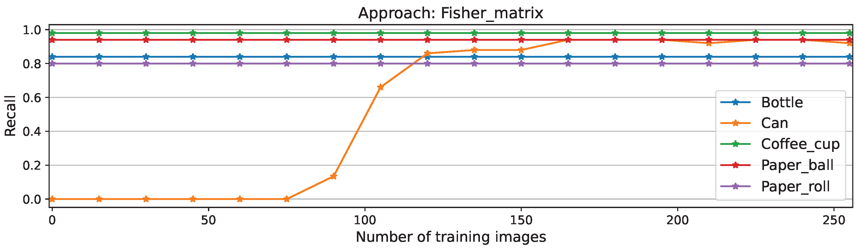

Table 1.
Material content of different datasets used on experiments.
| Dataset | Materials |
|---|---|
| Training | All excluding Cans |
| Validation | All excluding Cans |
| Testing | All excluding Cans |
| CL | Cans only |
| CL-Testing | All |
Disclaimer/Publisher’s Note: The statements, opinions and data contained in all publications are solely those of the individual author(s) and contributor(s) and not of MDPI and/or the editor(s). MDPI and/or the editor(s) disclaim responsibility for any injury to people or property resulting from any ideas, methods, instructions or products referred to in the content. |
© 2025 by the authors. Licensee MDPI, Basel, Switzerland. This article is an open access article distributed under the terms and conditions of the Creative Commons Attribution (CC BY) license (http://creativecommons.org/licenses/by/4.0/).
Copyright: This open access article is published under a Creative Commons CC BY 4.0 license, which permit the free download, distribution, and reuse, provided that the author and preprint are cited in any reuse.


