Submitted:
07 November 2025
Posted:
10 November 2025
You are already at the latest version
Abstract
Accurate forecasting of local weather patterns is essential for climate resilience and sustainable planning. This study analysed 35 years (1990--2025) of hourly temperature and precipitation data from Thohoyandou, South Africa, to assess the effects of climate change and improve anomaly prediction. Exploratory analysis and BEAST decomposition revealed accelerated warming trends of 0.025 °C per year in temperature anomalies, and irregular rainfall patterns dominated by extreme events rather than systematic changes. Two machine learning models, Artificial Neural Networks (ANN) and Long Short-Term Memory (LSTM) networks, were evaluated for anomaly forecasting, with feature selection guided by LASSO regression. For temperature, the LSTM model outperformed the ANN, achieving RMSE = 0.678, MAE = 0.466, and MASE = 0.520, compared to RMSE = 0.738, MAE = 0.524, and MASE = 0.585 for the ANN, with improvements confirmed by the Diebold--Mariano test. For precipitation, both models performed similarly, with the LSTM slightly better (RMSE = 0.432, MAE = 0.112, MASE = 1.897). These results highlight the LSTM model’s superior ability to capture temperature anomalies and the continued challenges of modelling rainfall, providing evidence-based insights to support agricultural planning, water management, and climate adaptation in Southern Africa.
Keywords:
BEAST
; climate change
; local weather patterns
; machine learning
; precipitation
; temperature
; Thohoyandou
1. Introduction
Climate change is one of the most pressing challenges of the 21st century, profoundly affecting natural environments, human societies, and economic systems. Over the past decades, human activities have significantly altered the atmospheric composition, primarily through greenhouse gas emissions from fossil fuel combustion, deforestation, and land-use changes [1]. These processes trap heat, causing global warming and intensifying climate variability [2]. Consequently, the frequency and intensity of daily temperature extremes have increased, while precipitation patterns have become more unpredictable and often more severe [3].
The impacts of these changes extend beyond environmental degradation, affecting agriculture, water resources, biodiversity, and human health, particularly in regions reliant on stable climatic conditions. Understanding local impacts is critical, as global and regional assessments often fail to capture microclimatic variability that shapes adaptation strategies at the community level [4]. Rural populations, for instance, perceive and experience climate change differently from urban populations, as their livelihoods are closely linked to agricultural productivity, water availability, and local ecosystem stability. Research indicates that rural communities often detect climate change through shifts in temperature and precipitation, including rising temperatures and declining or irregular rainfall [5]. These localised changes have direct consequences for crop yields, soil health, and water supply, yet are frequently underrepresented in large-scale climate analyses.
South Africa is particularly susceptible to climate variability due to its geographic and climatic diversity, combined with socio-economic inequalities that exacerbate vulnerability. National and provincial studies provide insights into general climate trends, but they often overlook the localised fluctuations that affect small towns and rural areas [6]. Thohoyandou, located in the Limpopo province, exemplifies such a region. Over the past decades, it has experienced significant variations in temperature and rainfall, which have implications for agriculture, water availability, biodiversity, and urban development [5]. Despite its role as a regional economic and agricultural hub, there remains a lack of detailed localised climate research, particularly with respect to temperature and precipitation dynamics. These gaps hinder the capacity of local authorities and communities to plan for and mitigate the adverse effects of climate change.
Forecasting local weather patterns presents significant challenges. Traditional statistical and time series models, including Autoregressive Integrated Moving Average (ARIMA), Seasonal ARIMA (SARIMA), and Generalised Autoregressive Conditional Heteroskedasticity (GARCH), are widely applied due to computational efficiency and interpretability [7]. However, these models rely on assumptions of linearity and stationarity, which often do not hold for climate variables characterised by complex, non-linear, and non-stationary behaviour. Similarly, Global Climate Models (GCMs) and statistical downscaling techniques provide useful projections but frequently fail to capture microclimatic variability at the scale of small towns, limiting their applicability for local adaptation and resource management [8]. These methodological limitations have driven the adoption of machine learning (ML) approaches, which can model non-linear relationships and detect intricate patterns in large datasets.
Machine learning and artificial intelligence techniques have demonstrated superior predictive performance compared to traditional statistical methods in diverse applications, including load forecasting and climate modelling [9,10]. In Africa, ML has been successfully applied to rainfall and temperature forecasting. Studies in East Africa using Random Forest, Support Vector Regression, Gradient Boosting, and XGBoost have demonstrated high predictive accuracy for short-term rainfall forecasts [11]. Research in West Africa employing recurrent neural networks (RNNs) and variants of the Kolmogorov-Arnold Network (KAN) has produced highly precise daily temperature and precipitation forecasts [12]. These studies highlight the ability of ML models to uncover hidden patterns, capture temporal dependencies, and improve forecast skill, particularly in contexts where traditional models struggle with data sparsity or complex environmental interactions.
Despite these advances, key research gaps remain. In South Africa, most studies focus on long-term climatic trends, drought monitoring, or agricultural impacts, with limited application of ML to jointly forecast temperature and rainfall at a local level. Where ML has been applied, analyses often target broad regions or single variables, overlooking the importance of joint forecasting in smaller towns. Furthermore, ML applications in Africa are concentrated in East and West Africa, leaving Southern Africa comparatively underexplored. While global studies indicate that deep learning methods such as Artificial Neural Networks (ANN) and Long Short-Term Memory (LSTM) networks can achieve high accuracy in climate forecasting, their use in localised African contexts remains rare. This underscores the need for studies that integrate advanced ML techniques with extensive local weather data to support local decision-making and resilience planning.
The impacts of climate change in Thohoyandou are further compounded by socio-economic vulnerabilities. Infrastructure, water supply, and food security are increasingly threatened, disproportionately affecting communities where poverty and inequality are prevalent [13]. Global climate models capture broad patterns but often fail to reflect localised trends critical for effective adaptation [2,14]. Applying ML algorithms to historical weather data allows detection of anomalies and subtle trends that may otherwise go unnoticed. The use of BEAST decomposition enables separation of systematic seasonal cycles from irregular events, providing a clear understanding of temperature and precipitation dynamics and supporting the identification of emergent patterns.
This study focuses on temperature and precipitation, two climate variables with direct implications for daily life, agriculture, and water resource management. Climate change has disrupted agricultural systems, affecting crop yields, pest and disease dynamics, and land productivity [10]. Rising temperatures contribute to more frequent and severe heatwaves, reducing soil moisture and increasing irrigation demand, while global warming is expected to produce more intense and irregular precipitation events [15,16]. By integrating anomaly detection, BEAST decomposition, and ML models (ANN and LSTM), this research seeks to improve forecasting accuracy and reveal local manifestations of climate change.
The findings of this study are expected to contribute significantly to both local and global discussions on climate resilience. By analysing temperature and precipitation anomalies, highlighting deviations from expected seasonal behaviour, and identifying emerging trends, the research provides actionable insights for agricultural planning, water management, and community-level adaptation. Moreover, it demonstrates the value of combining anomaly analysis, decomposition methods, and advanced machine learning for localised climate studies, addressing existing gaps in Southern African climate research and supporting evidence-based strategies for sustainable development and resilience planning.
1.1. Contribution and research highlights
The contributions and research highlights are given below.
1.1.1. Contributions
The main contributions of this study are:
- Provided a detailed, data-driven analysis of local climate change in Thohoyandou, South Africa, quantifying a persistent warming trend of 0.025°C per year and identifying erratic, highly variable precipitation patterns over 35 years.
- Demonstrated the superior capability of Long Short-Term Memory (LSTM) models over standard Artificial Neural Networks (ANNs) for forecasting temperature anomalies, while also highlighting the inherent challenges in modelling highly stochastic precipitation anomalies, where both models performed similarly.
1.1.2. Research highlights
- The study identified a persistent and accelerating warming trend in Thohoyandou, with temperatures rising by approximately 0.025°C per year, confirming regional climate change observations.
- Analysis revealed that rainfall has become increasingly variable, dominated by sporadic extreme events rather than systematic seasonal shifts, posing significant challenges for water resource management and agriculture.
- For temperature anomaly prediction, the LSTM model significantly outperformed the ANN, achieving lower error metrics (e.g., RMSE of 0.678 vs. 0.738). Its superiority was confirmed as statistically significant by the Diebold–Mariano test.
- For precipitation anomalies, the LSTM and ANN models showed no statistically significant difference in performance, underscoring the difficulty of forecasting highly stochastic and sporadic rainfall events.
- Feature selection identified lagged temperature and dew point variables as strong predictors for temperature anomalies, emphasising the role of temporal autocorrelation and atmospheric humidity.
- The LSTM model proved particularly effective in tracking sharp temperature fluctuations during critical events, such as heatwaves and cold snaps, highlighting its potential for practical climate risk management and early warning systems.
2. Materials and Methods
2.1. Study Area
The study focuses on Thohoyandou, located in the Limpopo Province of South Africa. Its precise geographical coordinates are longitude 30.4663°E and latitude -22.9749°S, and it lies at an elevation of approximately 596 metres above sea level. Thohoyandou experiences a subtropical climate, characterised by hot and humid summers and warm, dry winters, with marked seasonal variations in both temperature and rainfall [17].
The location was selected due to its complex local weather patterns and its significance within the wider context of climate variability in northern South Africa. Thohoyandou represents a data-scarce environment, making it an ideal case study for testing machine learning forecasting approaches.
Figure 1.
Location map of Thohoyandou, Limpopo Province, South Africa.

2.2. Data Source
The historical weather data used in this study, comprising hourly temperature (2 m) and precipitation (snow + rain) records over a 35-year period, were obtained from the Historical Weather API, available at https://open-meteo.com/en/docs/historical-weather-api. This API provides comprehensive long-term hourly climate records derived from global reanalysis datasets, offering high temporal resolution and consistency, making it suitable for detailed analysis of weather patterns and long-term climate trends.
The dataset contains 308,616 hourly observations collected between 1 January 1990 and 16 March 2025, representing 35 years of continuous monitoring for Thohoyandou. After feature engineering, the working dataset comprises 308,448 observations. The primary climate variables analysed are temperature (°C) and precipitation (mm), complemented by several engineered temporal features to enhance forecasting performance.
Data preprocessing focused on ensuring the accuracy and reliability of both variables. A key challenge was the predominance of zero values in the precipitation series, reflecting the frequent absence of rainfall typical of a subtropical climate. These zeros were retained, as their removal would have biased the analysis by excluding dry conditions. No imputation methods were applied, since modifying rainfall records could distort the natural distribution of events. Importantly, the dataset contained no missing values, ensuring complete temporal continuity across the 35-year observation period.
Temperature values exhibited continuous variation without zero-related issues. To better capture climate variability, temperature and precipitation anomalies were computed by subtracting the long-term mean from each hourly observation. These anomaly variables highlight unusual conditions, such as extreme heat or heavy rainfall, and provide centred series suitable for trend and forecasting analyses. Outliers were not removed, as they represent genuine extreme events, which are of particular importance in climate research.
2.3. Machine Learning Models
Two machine learning models were employed in this study: the Artificial Neural Network (ANN) and the Long Short-Term Memory (LSTM) network. The ANN served as a baseline model, while the LSTM was implemented as the primary forecasting model due to its superior ability to capture temporal dependencies.
2.3.1. Artificial Neural Network (ANN)
ANN was first developed in 1943 by [18], who introduced a mathematical model of a simplified artificial neuron. This early work laid the foundation for neural computation. In 1958, [19] developed the perceptron, the first algorithmically trainable neural network capable of performing binary classification. Its inefficacy in solving nonlinear problems diminished popularity until 1986 when David Rumelhart, Geoffrey Hinton, and Ronald Williams developed the backpropagation algorithm [20]. This breakthrough emerged with the ability to train multilayer neural networks by efficiently modifying the weights using the gradient descent optimisation technique. Backpropagation computes the gradient of the loss function concerning each network weight by transmitting error signals in reverse from the output layer back to the input layer. This advancement played a pivotal role in renewing interest in ANNs, ultimately paving the way for the emergence of deep learning models. Today, ANNs are extensively applied to various complex tasks, including image classification, natural language processing, and time series prediction.
A simple neural network in Mathematics can be defined as follows:
where (2) defines as the input to the neuron, as the weight linking input j to neuron k, and as the input feature. Equation (3) represents the threshold, denoted by . Figure 2 illustrates a multilayer feedforward ANN, comprising an input layer, hidden layers, and an output layer. This type of network contains three essential layers an input layer plus one or more hidden layers, and an output layer. Finally, Equation (4) includes , the activation function, which can be selected from various nonlinear functions such as the sigmoid function, ReLU, tanh, or others.
3. Feedforward Propagation
Feedforward propagation is how data travels through a neural network from start to finish. The information moves one way from the input layer, through any hidden layers, and finally to the output layer without looping back at any point. In each layer, the network calculates a weighted total of the inputs, combine a bias term, and then sends the result through an activation function to introduce nonlinearity.
The equations for the weighted input and activation of a neuron in a neural network are given by:
The variable represents the weighted input to neuron j, where is the weight connecting the input feature to neuron j, and is the corresponding bias term. The output (or activation) of neuron j is denoted by , which is obtained by applying the activation function , such as sigmoid, ReLU, or tanh, to the weighted input .
4. Backward Propagation
We first compute the error term at an output node j, where is the derivative of the activation function:
To propagate the error backward, we compute the error at a hidden node:
To adjust the weights and biases at any point in the network, we follow these update rules:
To adjust the weights and biases at the input layer, we use:
4.1. Long Short-Term Memory (LSTM) Network
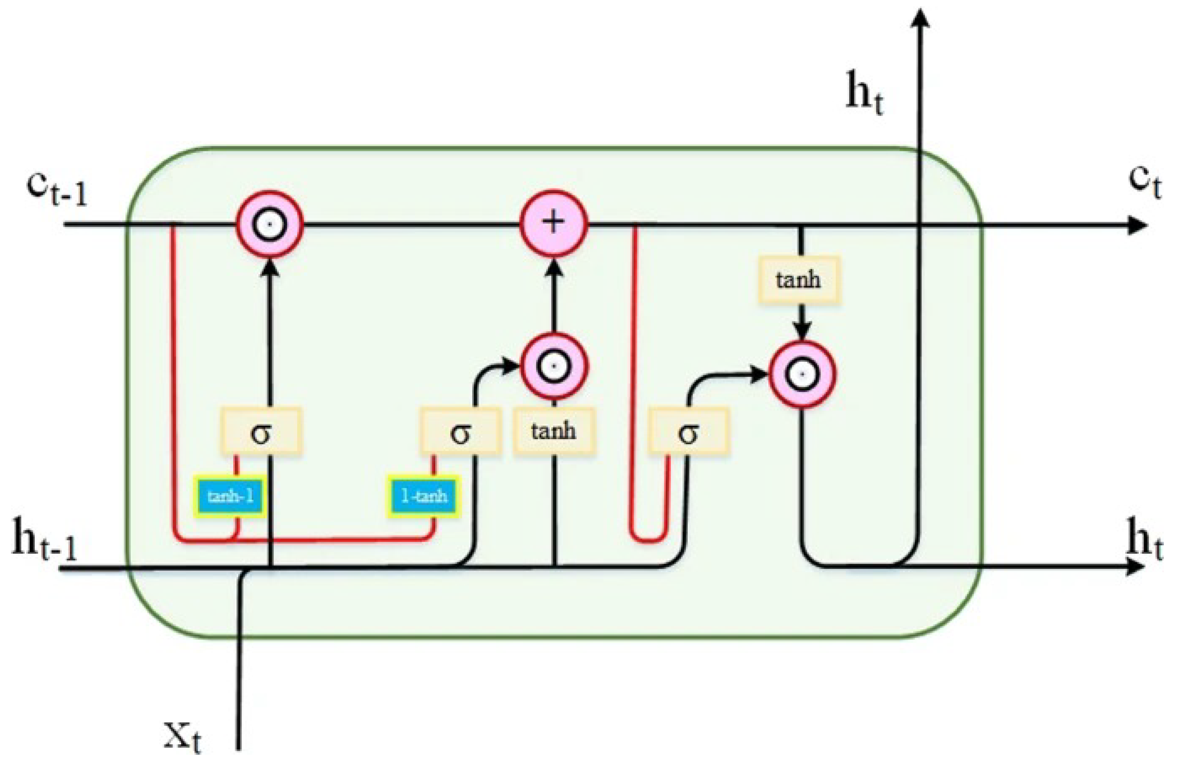
LSTM networks, a type of RNN, are designed to capture long-term dependencies in sequential data.What distinguishes LSTMs from traditional RNNs is their internal structure, which incorporates memory units called cells. These cells can control information flow using a system of gates: the input, forget, and output. This internal gating mechanism allows LSTMs to remember or discard information over extended sequences, solving the problem of shrinking gradients in deep neural networks that standard RNNs often face [22].
The forget gate is accountable for selecting which parts of the past information should be discarded. It does so by applying a logistic activation function to a combination of the previous hidden state and the current input:
moving on, the input gate determines which new information should be stored in the cell’s memory. This process is split into two steps: first, identifying the importance of the new input, and second, creating a vector of candidate data to be included in the memory.
These components are then used to update the cell memory. The past state is scaled by the forget gate’s output, while the input gate scales the new candidate information. Both are combined together to form the new memory:
Lastly, the output gate decides what the network should produce as output at the current time step. This is also a combination of the current input, the preceding hidden state, and the newly updated memory:
By dynamically regulating what information is stored, forgotten, or output at each time step, LSTMs are particularly effective for modelling data that involves temporal dependencies. This makes them highly suitable for applications such as weather forecasting, where patterns often evolve over long time horizons.
Figure 3.
Structure of LSTM [23].
Figure 3.
Structure of LSTM [23].
4.2. Variable Selection
Lasso regression, or Least Absolute Shrinkage and Selection Operator regression, is commonly applied in statistical modelling and machine learning. Lasso regression identifies variables and coefficients that reduce prediction error [24]. Its procedure’s popularity stems from its ability to decrease the regression coefficient vector towards zero and set some coefficients to zero, allowing for simultaneous estimation and variable selection [25]. The Lasso approach is beneficial for high-dimensional data with several predictor variables. It reduces the coefficients of irrelevant variables to zero, allowing for variable selection [24]. Lasso assists in identifying crucial principal components during the fitting of a regression model, not the original variables themselves. Lasso can be expressed in its most basic form as provided in [26]
where y is a response variable, and are measurements on the response variable, , ; , are the values that correspond to their respective k predictors, , are parameters, and denotes the error term.
4.3. Grid Search Optimisation
When building machine learning solutions, it is common practice to analyze different models to determine which one produces the best performance for a specific task. In this study, a model comprises a machine learning algorithm along with its adjustable parameters, which can be structural, such as the number of hidden layers or nodes, or algorithmic, such as the learning rate or mini-batch size. Hyperparameter optimisation is the process of discovering the optimal combination of structural and algorithmic parameters for a specific problem [27].
Hyperparameter tuning is an important stage since the hyperparameters chosen may greatly influence a model’s predictive results, including accuracy, generalisation, and convergence. Grid search is a popular method for hyperparameter tuning. It involves exhaustively training models with all possible combinations and identifying the configuration that performs best on a validation set [28]. This rigorous approach guarantees a thorough search of the hyperparameter space, resulting in a dependable strategy for optimizing machine learning models. Grid search was preferred over random search or Bayesian optimisation because it assures exhaustive evaluation across the stated parameter space, resulting in reliability in small-scale studies. Grid search was used in this study to adjust the hyperparameters of both the ANN and LSTM models, which resulted in optimal prediction performance.
4.4. Measures of Forecast Accuracy
Mean Absolute Error
Root Mean Square Error
Mean Bias Error
Mean Absolute Scaled Error
4.5. Diebold-Mariano Test
In addition to the standard evaluation metrics, it is important to test whether differences in forecast accuracy are statistically significant. To achieve this, we used the Diebold-Mariano (DM) test [29].
Let denote the observed GHI values at time t, and let represent the forecasts from model i. The forecast errors are defined as
If denotes a loss function, then a specification that penalises underprediction more heavily than overprediction can be expressed as
where is a penalty parameter and is the indicator function.
The loss differential between the two competing forecasts is then calculated as
The hypotheses of the DM test are defined as:
This test allows us to assess whether differences in forecast accuracy between ANN and LSTM are statistically significant, avoiding reliance on metrics alone.
4.6. Software Tools and Libraries
All analyses were conducted using Python (version 3.12), which handled data preprocessing, machine learning modelling, and visualisation. The primary Python libraries included pandas for data manipulation, NumPy for numerical computations, Matplotlib and Seaborn for graphical representation, and TensorFlow for implementing neural network architectures. R (version 4.3.1) was used specifically for the BEAST time series decomposition, which extracted the trend and seasonal components from the climatic data. The integration of Python and R facilitated a reproducible and efficient computational workflow.
5. Results
5.1. Data Overview and Statistical Properties
This section presents a detailed examination of the statistical characteristics of the 35-year hourly temperature and precipitation dataset for Thohoyandou. The objective is to understand the underlying data patterns, evaluate the distributional properties of the key variables, and verify their suitability for subsequent modelling.
As shown in Table 1, temperature values ranged from 4.4 °C to 41.3 °C, with a mean of 20.15 °C and a standard deviation of 5.38 °C, indicating moderate variability across the study period. The near-zero skewness (0.179) and slightly negative kurtosis (–0.240) suggest that the temperature distribution is approximately normal but marginally flatter (platykurtic). These characteristics align with the subtropical climate of Thohoyandou, which generally maintains warm conditions with moderate seasonal fluctuations. The computed temperature anomalies are properly standardised, with a mean of zero and moderate positive skewness (0.517), indicating slightly more frequent warm deviations.
In contrast, precipitation displays a highly skewed and leptokurtic distribution. Most hourly records show zero rainfall, with only a few intense events contributing to the total rainfall volume. The mean precipitation is 0.12 mm, but the maximum reaches 18.6 mm, confirming the intermittent nature of rainfall in the region. The extremely high skewness (10.804) and kurtosis (186.258) highlight the dominance of dry hours interspersed with occasional heavy rainfall, a pattern typical of subtropical summer climates. The precipitation anomaly distribution mirrors this behaviour, maintaining the same skewed shape, which indicates that anomaly standardisation preserved the natural variability of the rainfall data.
To further assess the temporal properties of the dataset, the Augmented Dickey-Fuller (ADF) and Kwiatkowski-Phillips-Schmidt-Shin (KPSS) tests were conducted on both temperature and precipitation anomaly series. These complementary statistical tests evaluate whether a time series is stationary or exhibits a deterministic trend. The ADF test assumes non-stationarity as its null hypothesis, whereas the KPSS test assumes stationarity, allowing for a more robust interpretation when used together.
As presented in Table 2, the ADF test rejects the null hypothesis of a unit root for both temperature and precipitation anomalies at the 5% significance level, confirming stationarity. However, the KPSS test rejects the null hypothesis of level stationarity, indicating the presence of deterministic trends within the data. Together, these results suggest that both variables exhibit trend-stationary behaviour where short-term fluctuations remain stable around a mean level, but a long-term trend persists. This trend-stationary nature reflects gradual climatic shifts in Thohoyandou over the 35-year observation period. Consequently, the detrended anomaly data are suitable for subsequent modelling and forecasting, as they retain meaningful temporal dependencies while satisfying the assumptions of statistical and machine learning approaches.
5.2. Exploratory Analysis of Temperature and Precipitation
Figure 4 shows the relationship between hourly temperature and precipitation over the 35-year period. Most observations cluster near zero precipitation, confirming that dry hours dominate. Temperature spans the full observed range regardless of rainfall, and no clear correlation is evident, indicating that short-term precipitation events occur largely independently of temperature. Occasional high-precipitation outliers correspond to rare but intense storm events.
Temporal dynamics over the full record are illustrated in Figure 5. Temperature exhibits pronounced seasonal and annual cycles, reflecting predictable climatological patterns, whereas precipitation is highly irregular, characterised by sporadic bursts of rainfall. Daily temperature cycles, such as diurnal heating and cooling, are also apparent in the data, though not shown here. These patterns indicate that temperature is systematic and predictable, while precipitation is stochastic and event-driven.
Figure 6 presents density and Q-Q plots for temperature and precipitation, highlighting differences in distribution. Temperature approximates a normal distribution centered around 20–25 °C, whereas precipitation is strongly right-skewed with many zeros and a long tail of extreme events. Seasonal trends in temperature are apparent, with summer months reaching higher values and winter months lower ones, while transitional months show greater variability. Precipitation, in contrast, lacks a consistent monthly pattern and is dominated by zeros with occasional extreme rainfall hours. These observations justify modeling temperature using approaches assuming near-normality and precipitation using methods that accommodate zero inflation and heavy tails.
Temperature and precipitation anomalies relative to the 35-year mean are shown in Figure 7 and Figure 8, respectively. Temperature anomalies fluctuate around zero but display more frequent positive deviations in recent years, indicating a gradual warming trend. Precipitation anomalies remain highly irregular, dominated by sporadic extreme events, with no clear long-term trend. These results emphasise that temperature changes are progressive and predictable, whereas precipitation remains highly variable and event-driven.
5.3. BEAST Decomposition and change point Detection
To examine long-term climate changes in Thohoyandou, the Bayesian Estimator of Abrupt change, Seasonal change, and Trend (BEAST) was applied to temperature and precipitation anomalies. BEAST decomposes time series into trend, seasonal, and residual components while detecting abrupt change points using Bayesian model averaging, which accounts for model uncertainty [30].
Figure 9.
BEAST decomposition for temperature and precipitation anomalies in Thohoyandou (1990–2025).
Figure 9.
BEAST decomposition for temperature and precipitation anomalies in Thohoyandou (1990–2025).
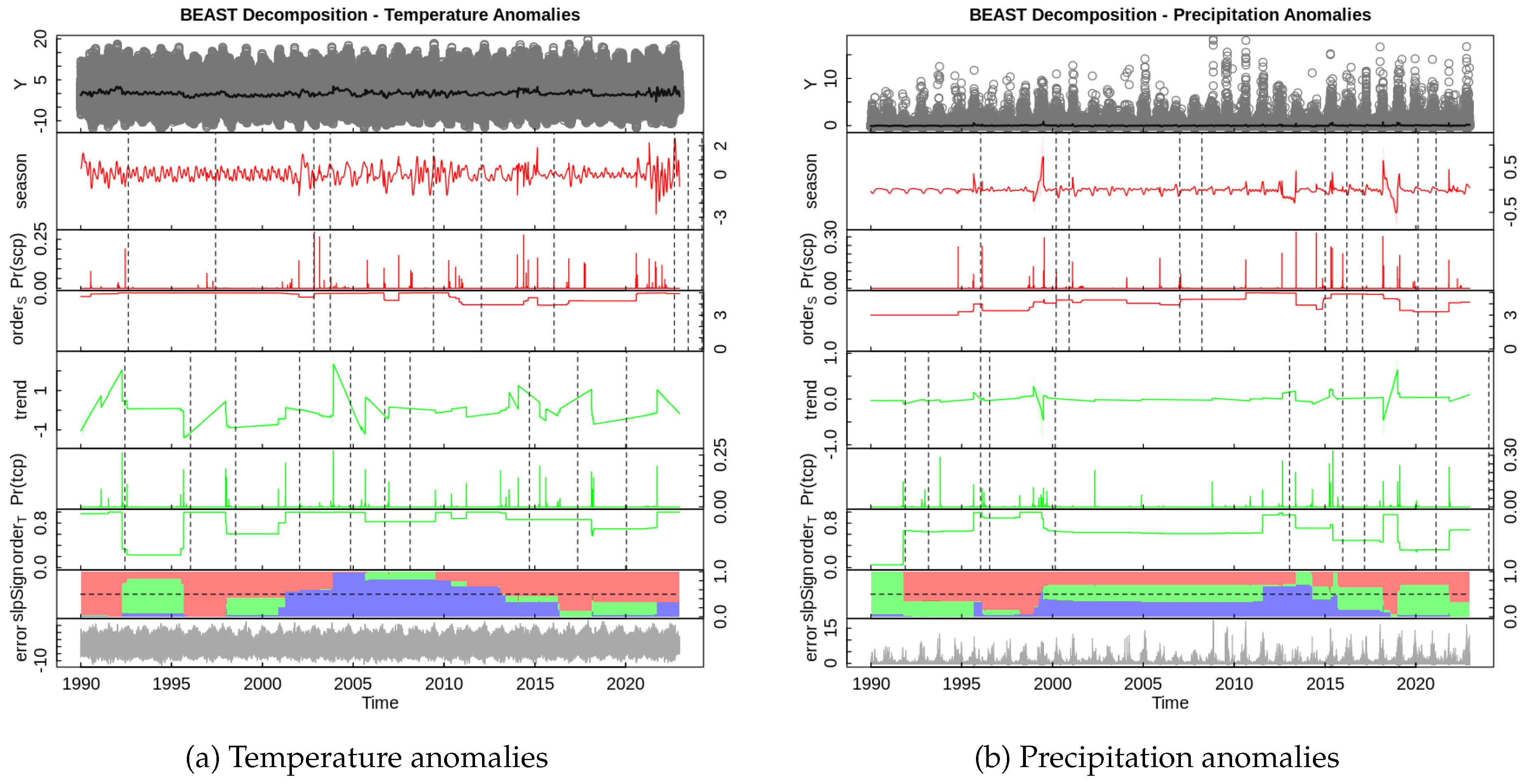
Table 3 summarizes the detected trends and change points. Temperature anomalies increase at 0.0250 °C per year, with change points detected between 1992 and 2020, indicating accelerated warming beyond normal seasonal variability. Precipitation anomalies show a small upward trend of 0.0037 mm per year, with change points between 1991 and 2024, reflecting occasional abrupt shifts in rainfall patterns.
These results suggest that temperature in Thohoyandou is rising steadily, with noticeable periods of abrupt warming likely linked to climatic events such as El Niño or anthropogenic influences. Precipitation remains largely irregular, with sudden changes, highlighting the challenges in predicting rainfall patterns. Overall, monitoring both trends and abrupt shifts is crucial for climate adaptation and resilience planning in the region.
5.4. Correlation Analysis
Figure 10 shows Correlation analysis reveals that temperature anomalies are strongly related to temperature () and negatively correlated with relative humidity (), with moderate positive correlation with dew point. Precipitation anomalies are highly correlated with precipitation () but show weak correlations with other meteorological variables. Calendar variables (day, month, hour) have minimal correlation with either anomaly. Temperature variability is systematic and influenced by multiple factors, whereas precipitation remains largely stochastic. These patterns justify the use of lagged temperature and precipitation anomalies as dominant predictors in subsequent feature engineering and LASSO-based model selection.
5.5. Feature Engineering and Variable Selection
To capture temporal dependencies, lagged features were created: temperature anomaly (lags 1, 2, 3, 168 hours) and precipitation anomaly (lags 1, 2, 3, 24 hours). Calendar variables and other meteorological covariates (humidity, dew point, cloud cover, wind speed/direction, pressure) were also included.
LASSO regression with five-fold cross-validation selected predictors with non-zero coefficients. Figure 11 and Figure 12 show the results. Temperature anomaly is strongly influenced by lag1, dew point, and lag168, while precipitation anomaly is dominated by lag1, with minor contributions from lag3 and lag24. Calendar and other meteorological variables contribute minimally.
5.6. Machine Learning Models
The dataset was divided into a 90%-10% ratio for training and testing, respectively. Two machine learning models were developed: an Artificial Neural Network (ANN) and a Long Short-Term Memory (LSTM) network. Before training, predictor variables were normalised, and feature selection was conducted using LASSO regression to retain the most relevant variables. Model hyperparameters were optimised through grid search combined with early stopping, ensuring optimal performance while mitigating overfitting. The predictive accuracy of both models was then evaluated on the test set to assess their ability to capture temporal variability in temperature and precipitation anomalies.
5.6.1. Model Hyperparameter Selection
Table 4 summarises the optimal hyperparameters for the ANN and LSTM models. These configurations were determined through grid search and early stopping, balancing predictive accuracy and overfitting prevention. For temperature anomalies, both models used 64 units, a dropout rate of 0.2, and a learning rate of 0.001. The precipitation models required slightly different configurations, particularly a reduced number of epochs and a smaller learning rate for the LSTM. Presenting these hyperparameters provides transparency and reproducibility for the model development process.
5.6.2. Temperature Anomaly Forecasting
Table 5 presents the predictive performance of the ANN and LSTM models on the test set using RMSE, MAE, MBE, and MASE. The LSTM model outperformed the ANN across most metrics, indicating a stronger ability to capture the temporal patterns in temperature anomalies. Specifically, the LSTM achieved a lower RMSE of 0.678 and MAE of 0.466, compared to the ANN with RMSE of 0.738 and MAE of 0.524.
The MBE values indicate slight overprediction for both models, with ANN at 0.070 and LSTM at 0.123, showing a small positive bias. Both models achieved MASE values below 1, with LSTM at 0.520, demonstrating better performance than a naïve one-step-ahead forecast. These results suggest that the LSTM provides slightly more accurate predictions for temperature anomalies, making it more reliable for capturing unusual climatic conditions such as heatwaves or cold snaps.
Figure 13 compares the actual temperature anomalies with predictions from both models. The LSTM predictions closely track the observed anomalies, particularly during periods of rapid change, while ANN predictions show slightly larger deviations. For example, during known heatwave periods or unseasonal cold events, the LSTM was able to follow the sharp increases or decreases in temperature anomalies more accurately than the ANN, highlighting its potential for practical applications in climate monitoring and forecasting.
The Diebold–Mariano (DM) test in Table 6 confirms that the predictive accuracy of the LSTM is statistically superior to that of the ANN (DM = 28.35, p-value < 0.001). Given the near-zero p-value, the null hypothesis of equal predictive accuracy is rejected, indicating that the LSTM model significantly outperforms the ANN in forecasting temperature anomalies. The LSTM’s ability to model long-term dependencies allows it to better capture sharp variations in temperature anomalies, as also shown in Figure 13.
Figure 14 provides a zoomed-in comparison between LSTM predictions and observed temperature anomalies. The close alignment between predicted and actual values highlights the LSTM’s ability to capture both the timing and magnitude of rapid temperature fluctuations. This detailed view, alongside the statistically significant results from the Diebold–Mariano test (Table 6) and performance metrics (Table 5), reinforces the LSTM’s suitability for climate anomaly forecasting.
5.6.3. Precipitation Anomaly Forecasting
The study proceeded to select optimal hyperparameters for both the ANN and LSTM models in forecasting precipitation anomalies. To ensure a fair comparison, the same hyperparameter tuning techniques applied to the temperature anomaly models were employed. Specifically, grid search and early stopping were used to identify configurations that maximised validation performance while minimising overfitting. The resulting optimal hyperparameters are summarised in Table 4 and were subsequently used to train the precipitation models. These carefully selected configurations guarantee consistency and fairness in evaluating the predictive performance of the ANN and LSTM models on the precipitation dataset. The performance of the models on the test set demonstrates their effectiveness in capturing precipitation anomalies and provides a reliable basis for comparison between the ANN and LSTM approaches.
Table 7 presents the predictive performance of the ANN and LSTM models on the test set using RMSE, MAE, MBE, and MASE. The LSTM model slightly outperformed the ANN across most metrics, indicating a stronger ability to capture temporal patterns in the data. Specifically, the LSTM achieved a lower RMSE of 0.432 and MAE of 0.1124, compared to the ANN with RMSE of 0.434 and MAE of 0.1279. The MBE values were close to zero for both models, with 0.0097 for the ANN and 0.0100 for the LSTM, indicating minimal systematic overprediction or underprediction. The positive MBE for the ANN suggests a slight overprediction, while the negative MBE for the LSTM indicates a slight underprediction. Both models achieved MASE values above 1, with the LSTM achieving a lower value of 1.8971 compared to 2.1583 for the ANN, demonstrating relatively better accuracy compared to a na¨ıve benchmark forecast.
Figure 15 compares the actual values with predictions from both models. The LSTM predictions follow the observed values more closely, particularly during periods of rapid change, whereas the ANN predictions exhibit slightly larger deviations. These results suggest that the LSTM provides superior predictive performance, likely due to its ability to model temporal dependencies in the data more effectively than the standard ANN.
The DM test results in Table 8 indicate that the differences in forecast accuracy between the ANN and LSTM models for precipitation anomalies are not statistically significant (DM = 0.434, p = 0.664). Since the p-value is well above conventional significance levels (0.01, 0.05, 0.10), the null hypothesis of equal predictive performance cannot be rejected. This suggests that, despite minor variations in performance metrics, both models perform comparably. The high variability and sporadic nature of precipitation, characterised by numerous zero or low values interspersed with occasional bursts, likely contribute to the similar performance, making it difficult for either model to consistently outperform the other.
Figure 16 presents a detailed comparison of precipitation anomaly predictions from the ANN and LSTM models, allowing a detailed comparison despite the lack of statistically significant differences. This closer inspection reveals how each model captures rapid fluctuations and subtle variations that full-range plots may obscure. Although the DM test shows comparable performance, visualising the models side by side highlights their behaviour during critical periods and underscores the challenges of modelling highly variable precipitation anomalies, complementing the quantitative metrics with richer insight.
6. Discussion
The findings of this study provide significant insights into how local weather patterns in Thohoyandou have evolved over the past 35 years, influenced by climate change. The BEAST decomposition results show a persistent warming trend of approximately 0.025 °C per year, confirming the acceleration of temperature increases in northern South Africa. This aligns with previous studies that identified similar warming rates across Southern Africa, where rising minimum and maximum temperatures are among the most consistent indicators of climate change (Ziervogel et al. and Stott, [3,13]). The observed trend further corroborates the findings of Mzezewa and Gwata [17], who reported an increase in heat stress and a decline in soil moisture in semi-arid regions, resulting in a higher irrigation demand and increased crop vulnerability.
The irregular and highly skewed nature of precipitation patterns observed in this study supports earlier research indicating that rainfall variability in Southern Africa has intensified rather than decreased [14,16]. The detected change points between 1991 and 2024 reflect the erratic behaviour of rainfall events, suggesting that precipitation in Thohoyandou is increasingly dominated by sporadic extremes rather than systematic seasonal shifts. This finding aligns with results from Davenport and Diffenbaugh [15], who discovered that extreme precipitation events in subtropical climates are becoming more frequent and less predictable. These findings underscore the need to integrate stochastic rainfall modelling and anomaly detection methods into local climate forecasting systems.
From a methodological perspective, the study demonstrates that Long Short-Term Memory (LSTM) networks outperform standard Artificial Neural Networks (ANNs) in forecasting temperature anomalies, as evidenced by lower RMSE, MAE, and MASE values, and a statistically significant Diebold–Mariano test (p < 0.001). This result is consistent with prior work by Alizadegan et al. [22], who showed that LSTMs achieve superior predictive accuracy in time series tasks involving long-term dependencies. The superior performance of the LSTM model suggests that temporal memory mechanisms are essential for capturing the persistence and gradual nature of temperature anomalies. In contrast, the comparable performance of ANN and LSTM models in precipitation forecasting reflects the stochastic and event-driven nature of rainfall, which limits the benefits of deep temporal modelling. This finding aligns with Gwahwera et al. [11], who observed that machine learning models often struggle to accurately predict sporadic precipitation due to noise and zero inflation in rainfall datasets.
The results also underscore the importance of feature engineering and LASSO-based variable selection in enhancing model interpretability. Lagged temperature and dew point variables emerged as strong predictors of temperature anomalies, reaffirming the role of atmospheric humidity and temporal autocorrelation in explaining local temperature fluctuations. However, precipitation forecasting remains more challenging, as rainfall patterns are driven by complex and often exogenous processes such as mesoscale convective systems and regional atmospheric circulation.
Beyond the methodological implications, these findings have substantial practical relevance. The identified warming trends and irregular rainfall patterns pose significant risks to agricultural productivity, water resource management, and infrastructure planning in Thohoyandou. Increasing temperature anomalies could intensify evapotranspiration and soil desiccation, while the unpredictability of rainfall could disrupt crop planting schedules and water storage systems. These localised findings contribute to the broader understanding of climate variability in Southern Africa and support the development of context-specific adaptation strategies.
Future research should focus on expanding the spatial scope of analysis to include neighbouring regions in Limpopo Province and integrating additional climatic variables such as wind speed, pressure, and soil moisture. Incorporating hybrid modelling approaches that combine physical climate models with data-driven deep learning frameworks could further enhance forecasting skills. Additionally, investigating explainable AI techniques would provide valuable insights into the underlying drivers of anomaly formation, improving trust and applicability of machine learning models in climate risk management.
This study demonstrates that machine learning, particularly LSTM networks, can effectively model complex temporal patterns in local climate data, offering a valuable complement to traditional statistical and dynamical methods. The results underscore the importance of local-scale analysis in understanding the nuanced impacts of global climate change and offer actionable insights for building climate resilience in data-scarce regions, such as Thohoyandou.
7. Conclusions
This study examined the evolution of local weather patterns in Thohoyandou, South Africa, over the past 35 years, with a focus on temperature and precipitation anomalies as indicators of climate change. Using BEAST decomposition and machine learning techniques, the research identified a clear warming trend of approximately 0.025 °C per year and irregular rainfall patterns characterised by extreme, event-driven variability rather than systematic change. These findings confirm that Thohoyandou, like much of Southern Africa, is experiencing accelerating temperature increases and increasingly unpredictable precipitation.
Among the forecasting models evaluated, the Long Short-Term Memory (LSTM) network consistently outperformed the Artificial Neural Network (ANN) in predicting temperature anomalies, demonstrating its ability to capture long-term temporal dependencies. However, both models exhibited similar performance in rainfall forecasting, reflecting the stochastic nature of precipitation. The results highlight that while deep learning can effectively model temperature trends, rainfall prediction remains challenging due to inherent variability and data sparsity.
Beyond methodological insights, the study provides valuable evidence for climate adaptation planning. The warming trend and irregular rainfall patterns pose significant risks to agriculture, water availability, and infrastructure in Thohoyandou. Local authorities and policymakers can utilise these findings to inform climate resilience strategies, including enhanced water resource management, adaptive agricultural practices, and infrastructure design tailored to more frequent temperature extremes and erratic rainfall events.
Future work should extend this analysis to a broader spatial scale across Limpopo Province, incorporate additional atmospheric and soil variables, and test hybrid modelling frameworks that combine physical climate models with machine learning. Such approaches would enhance interpretability, reliability, and applicability in climate impact assessment and local-level forecasting. Overall, this study demonstrates the power of combining data-driven and statistical approaches to understand better and anticipate local manifestations of global climate change.
Author Contributions
Conceptualisation, M.M., C.S., and T.R.; methodology, M.M.; software, M.M.; validation, M.M., C.S., and T.R.; formal analysis, M.M.; investigation, M.M., C.S., and T.R.; data curation, M.M.; writing—original draft preparation, M.M.; writing—review and editing, M.M., C.S., and T.R.; visualisation, M.M.; supervision, C.S. and T.R.; project administration, C.S. and T.R.; funding acquisition, M.M. All authors have read and agreed to the published version of this manuscript.
Funding
This research was funded by the DST-CSIR National e-Science Postgraduate Teaching and Training Platform (NEPTTP): http://www.escience.ac.za/, accessed on 15 January 2025.
Institutional Review Board Statement
Not applicable.
Informed Consent Statement
Not applicable.
Data Availability Statement
The historical weather data used in this study, comprising hourly temperature (2 m) and precipitation (snow + rain) records over a 35-year period, were obtained from the Historical Weather API, available at https://open-meteo.com/en/docs/historical-weather-api.(accessed on 5 February 2025). The analytic data and data in brief can be accessed from https://github.com/csigauke/.
Acknowledgments
The support of the DST-CSIR National e-Science Postgraduate Teaching and Training Platform (NEPTTP) provided for this research is acknowledged. The opinions expressed and conclusions arrived at are those of the authors and are not necessarily to be attributed to the NEPTTP. In addition, the authors thank the anonymous reviewers for their helpful comments on this paper.
Conflicts of Interest
The authors declare no conflicts of interest. The funders had no role in this study’s design; in the collection, analyses, or interpretation of data; in the writing of this manuscript; or in the decision to publish the results.
Abbreviations
The following abbreviations are used in this manuscript:
| ANN | Artificial Neural Network |
| BEAST | Bayesian Estimator of Abrupt change, Seasonal change, and Trend |
| DM | Diebold–Mariano |
| GARCH | Generalized Autoregressive Conditional Heteroskedasticity |
| LASSO | Least Absolute Shrinkage and Selection Operator |
| LSTM | Long Short-Term Memory |
| MAE | Mean Absolute Error |
| MASE | Mean Absolute Scaled Error |
| MBE | Mean Bias Error |
| ML | Machine Learning |
| RMSE | Root Mean Square Error |
| SARIMA | Seasonal Autoregressive Integrated Moving Average |
References
- Angra, D.; Sapountzaki, K. Climate change affecting forest fire and flood risk: Facts, predictions, and perceptions in central and South Greece. Sustainability 2022. [Google Scholar] [CrossRef]
- Romm, J. Climate Change: What Everyone Needs to Know; Oxford University Press: Oxford, UK, 2022. [Google Scholar]
- Stott, P. How climate change affects extreme weather events. Science 2016, 352, 1517–1518. [Google Scholar] [CrossRef]
- Hulme, M. Climate change isn’t everything: Liberating climate politics from alarmism. John Wiley & Sons, 2023.
- Rankoana, S.A. Perceptions of climate change and the potential for adaptation in a rural community in Limpopo Province, South Africa. Sustainability 2016, 8, 672. [Google Scholar] [CrossRef]
- Nkamisa, M.; Ndhleve, S.; Nakin, M.D.; Mngeni, A.; Kabiti, H.M. Analysis of trends, recurrences, severity and frequency of droughts using standardised precipitation index: Case of OR Tambo District Municipality, Eastern Cape, South Africa. J`amb´a-Journal of Disaster Risk Studies 2022, 14, 1147. [Google Scholar] [CrossRef]
- Han, H.; Liu, Z.; Barrios Barrios, M.; Li, J.; Zeng, Z.; Sarhan, N.; Awwad, E.M. Time series forecasting model for non-stationary series pattern extraction using deep learning and GARCH modeling. Journal of Cloud Computing 2024, 13, 2. [Google Scholar] [CrossRef]
- Hernanz, A.; García-Valero, J.A.; Domínguez, M.; Rodríguez-Camino, E. A critical view on the suitability of machine learning techniques to downscale climate change projections: Illustration for temperature with a toy experiment. Atmospheric Science Letters 2022, 23, e1087. [Google Scholar] [CrossRef]
- Yang, L.; Guo, J.; Tian, H.; Liu, M.; Huang, C.; Cai, Y. Multi-scale building load forecasting without relying on weather forecast data: A temporal convolutional network, long short-term memory network, and self-attention mechanism approach. Buildings 2025, 15, 298. [Google Scholar] [CrossRef]
- Talasila, P.; Potta, T.; Puppala, L.; Puligadda, N.B.P. Analysing the effect of climate change on crop yield using machine learning techniques. SSRN 4802729 2024. [Google Scholar] [CrossRef]
- Gahwera, T.A.; Eyobu, O.S.; Isaac, M. Analysis of machine learning algorithms for prediction of short-term rainfall amounts using Uganda’s Lake Victoria Basin weather dataset. IEEE Access 2024, 12, 63361–63380. [Google Scholar] [CrossRef]
- Akazan, A.-C.; Mbingui, V.R.; N’guessan, G.L.R.; Karambal, I. Localized weather prediction using Kolmogorov-Arnold network-based models and deep RNNs. arXiv preprint arXiv:2505.22686, 2025. [CrossRef]
- Ziervogel, G.; New, M.; Archer van Garderen, E.; Midgley, G.; Taylor, A.; Hamann, R.; Stuart-Hill, S.; Myers, J.; Warburton, M. Climate change impacts and adaptation in South Africa. Wiley Interdisciplinary Reviews: Climate Change 2014, 5, 605–620. [Google Scholar] [CrossRef]
- Giorgi, F. Thirty years of regional climate modeling: Where are we and where are we going next? Journal of Geophysical Research: Atmospheres 2019, 124, 5696–5723. [Google Scholar] [CrossRef]
- Davenport, F.V.; Diffenbaugh, N.S. Using machine learning to analyze physical causes of climate change: A case study of US Midwest extreme precipitation. Geophysical Research Letters 2021, 48, e2021GL093787. [Google Scholar] [CrossRef]
- Zhou, J.; Teuling, A.J.; Seneviratne, S.I.; Hirsch, A.L. Soil moisture–temperature coupling increases population exposure to future heatwaves. Earth’s Future 2024, 12, e2024EF004697. [Google Scholar] [CrossRef]
- Mzezewa, J.; Gwata, E. The nature of rainfall at a typical semi-arid tropical ecotope in Southern Africa and options for sustainable crop production. Crop Production Technologies 2012, pp. 95–112.
- McCulloch, W.S.; Pitts, W. A logical calculus of the ideas immanent in nervous activity. The Bulletin of Mathematical Biophysics 1943, 5, 115–133. [Google Scholar] [CrossRef]
- Rosenblatt, F. The perceptron: a probabilistic model for information storage and organization in the brain. Psychological Review 1958, 65(6). [Google Scholar] [CrossRef]
- Rumelhart, D.E.; Hinton, G.E.; Williams, R.J. Learning representations by back-propagating errors. Nature 1986, 323(6088), 533–536. [Google Scholar] [CrossRef]
- GeeksforGeeks. What is LSTM—Long Short Term Memory? GeeksforGeeks, 2024. Available online: https://www.geeksforgeeks.org/what-is-lstm-long-short-term-memory/ (accessed on 9 May 2025).
- Alizadegan, H.; Rashidi Malki, B.; Radmehr, A.; Karimi, H.; Ilani, M.A. Comparative study of long short-term memory (LSTM), bidirectional LSTM, and traditional machine learning approaches for energy consumption prediction. Energy Exploration & Exploitation 2025, 43(1), 281–301. [Google Scholar] [CrossRef]
- Yang, H.; Hu, J.; Cai, J.; Wang, Y.; Chen, X.; Zhao, X.; Wang, L. A new MC-LSTM network structure designed for regression prediction of time series. Neural Processing Letters 2023, 55(7), 8957–8979. [Google Scholar] [CrossRef]
- Ranstam, J.; Cook, J.A. Lasso regression. Journal of British Surgery 2018, 105(10), 1348–1348. [Google Scholar] [CrossRef]
- Hans, C. Bayesian lasso regression. Biometrika 2009, 96(4), 835–845. [Google Scholar] [CrossRef]
- Jolliffe, I.T.; Trendafilov, N.T.; Uddin, M. A modified principal component technique based on the LASSO. Journal of Computational and Graphical Statistics 2003, 12(3), 531–547. [Google Scholar] [CrossRef]
- Soper, D.S. Greed is good: Rapid hyperparameter optimization and model selection using greedy k-fold cross validation. Electronics 2021, 10(16), 1973. [Google Scholar] [CrossRef]
- Jiang, X.; Xu, C. Deep learning and machine learning with grid search to predict later occurrence of breast cancer metastasis using clinical data. Journal of Clinical Medicine 2022, 11(19), 5772. [Google Scholar] [CrossRef]
- Ranganai, E.; Sigauke, C. Capturing long-range dependence and harmonic phenomena in 24-hour solar irradiance forecasting: A quantile regression robustification via forecasts combination approach. IEEE Access 2020, 8, 172204–172218. [Google Scholar] [CrossRef]
- Zhao, K.; Wulder, M.A.; Hu, T.; Bright, R.; Wu, Q.; Qin, H.; Li, Y.; Toman, E.; Mallick, B.; Zhang, X.; et al. Detecting change-point, trend, and seasonality in satellite time series data to track abrupt changes and nonlinear dynamics: A Bayesian ensemble algorithm. Remote Sensing of Environment 2019, 232, 111181. [Google Scholar] [CrossRef]
Figure 2.
structure of multilayer neural network sourced from [21].
Figure 2.
structure of multilayer neural network sourced from [21].

Figure 4.
Scatterplot of temperature versus precipitation (1990–2025).
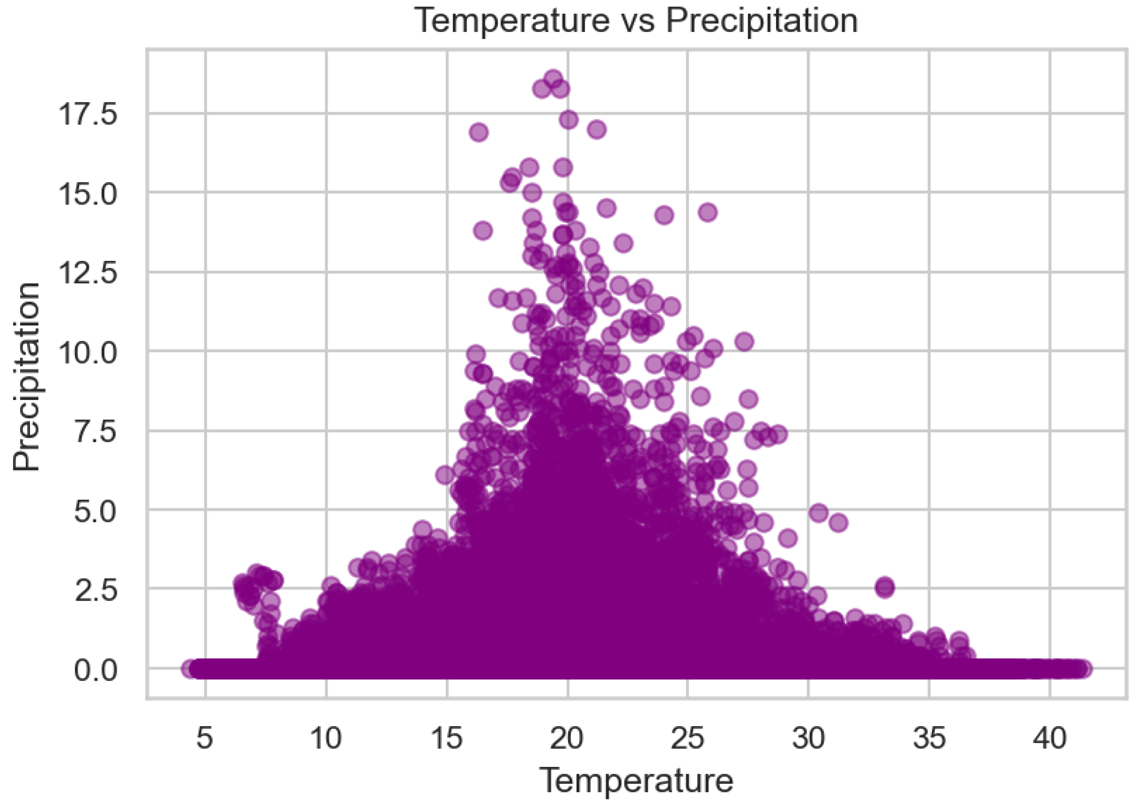
Figure 5.
Time series of hourly temperature and precipitation (1990–2025).
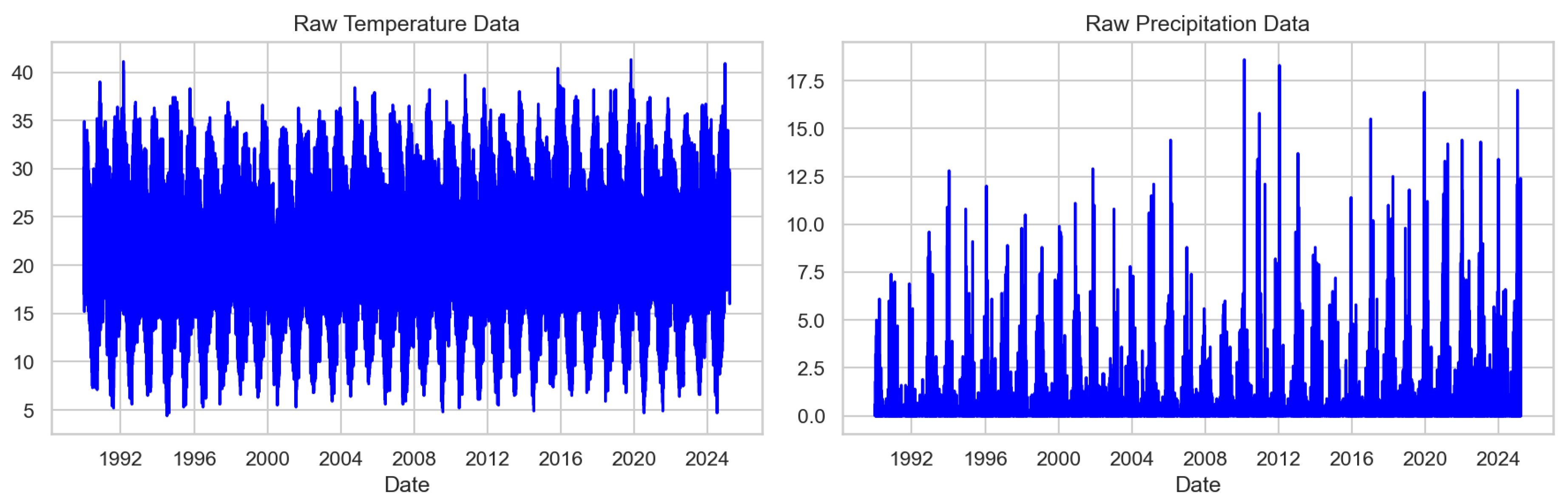
Figure 6.
Density and Q-Q plots of temperature and precipitation.
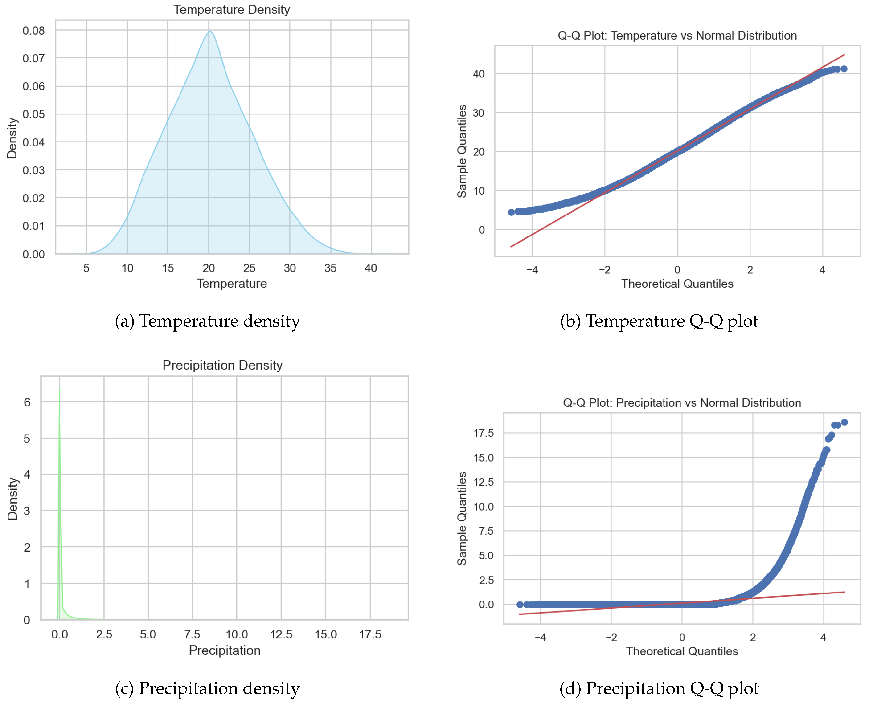
Figure 7.
Time series of temperature anomalies (1990–2025).
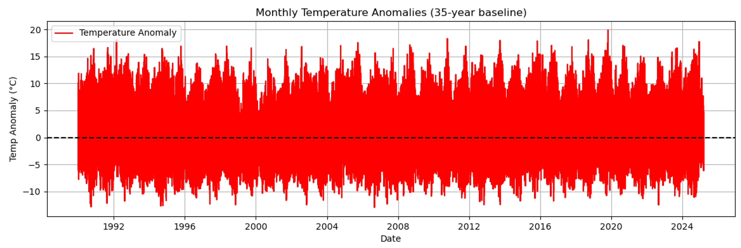
Figure 8.
Time series of precipitation anomalies (1990–2025).
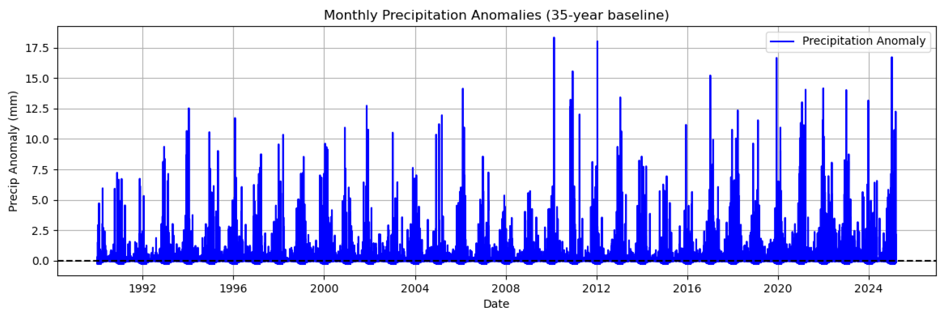
Figure 10.
Correlation heatmap of meteorological variables and anomalies.
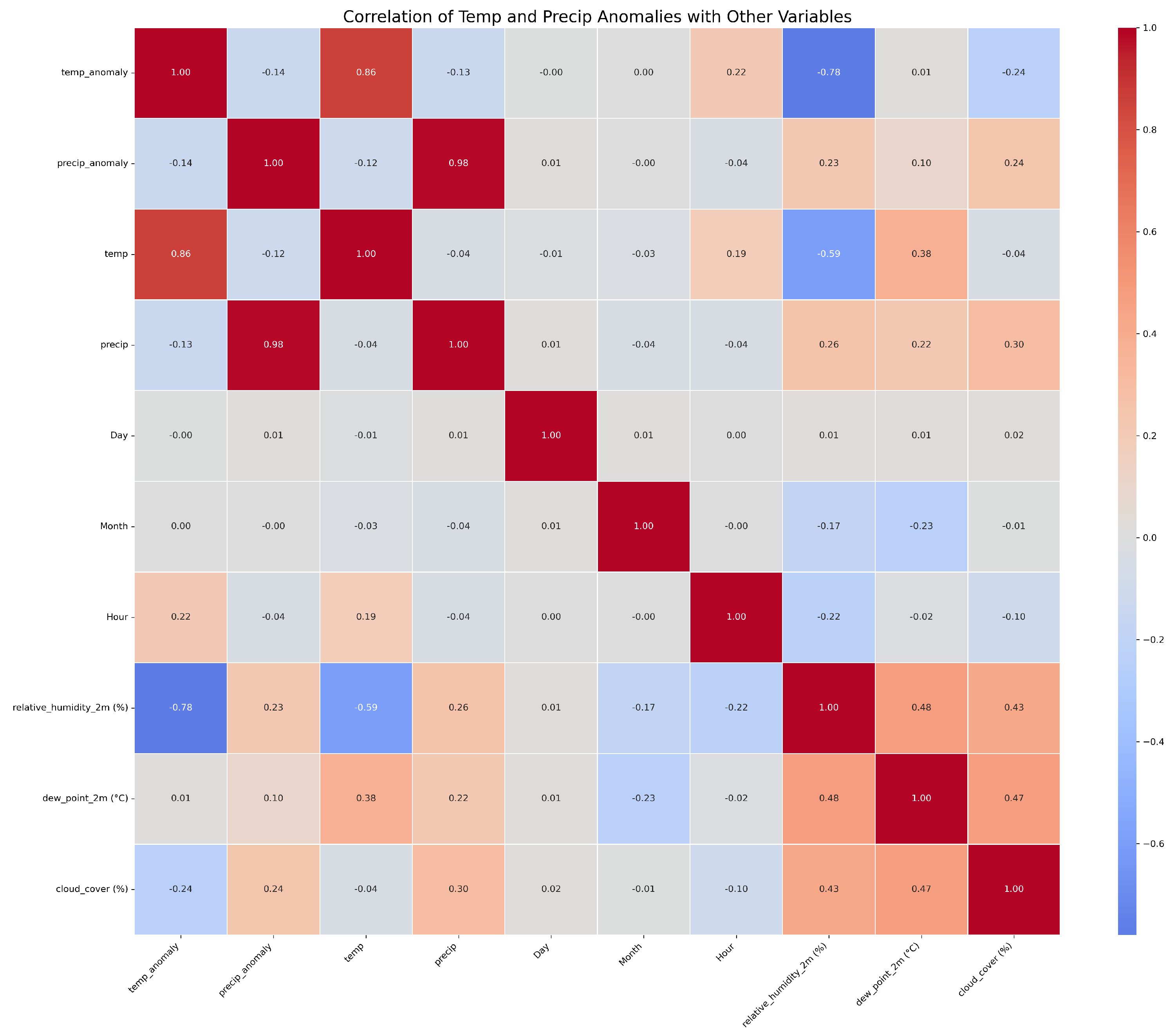
Figure 11.
Feature selection for temperature anomaly.
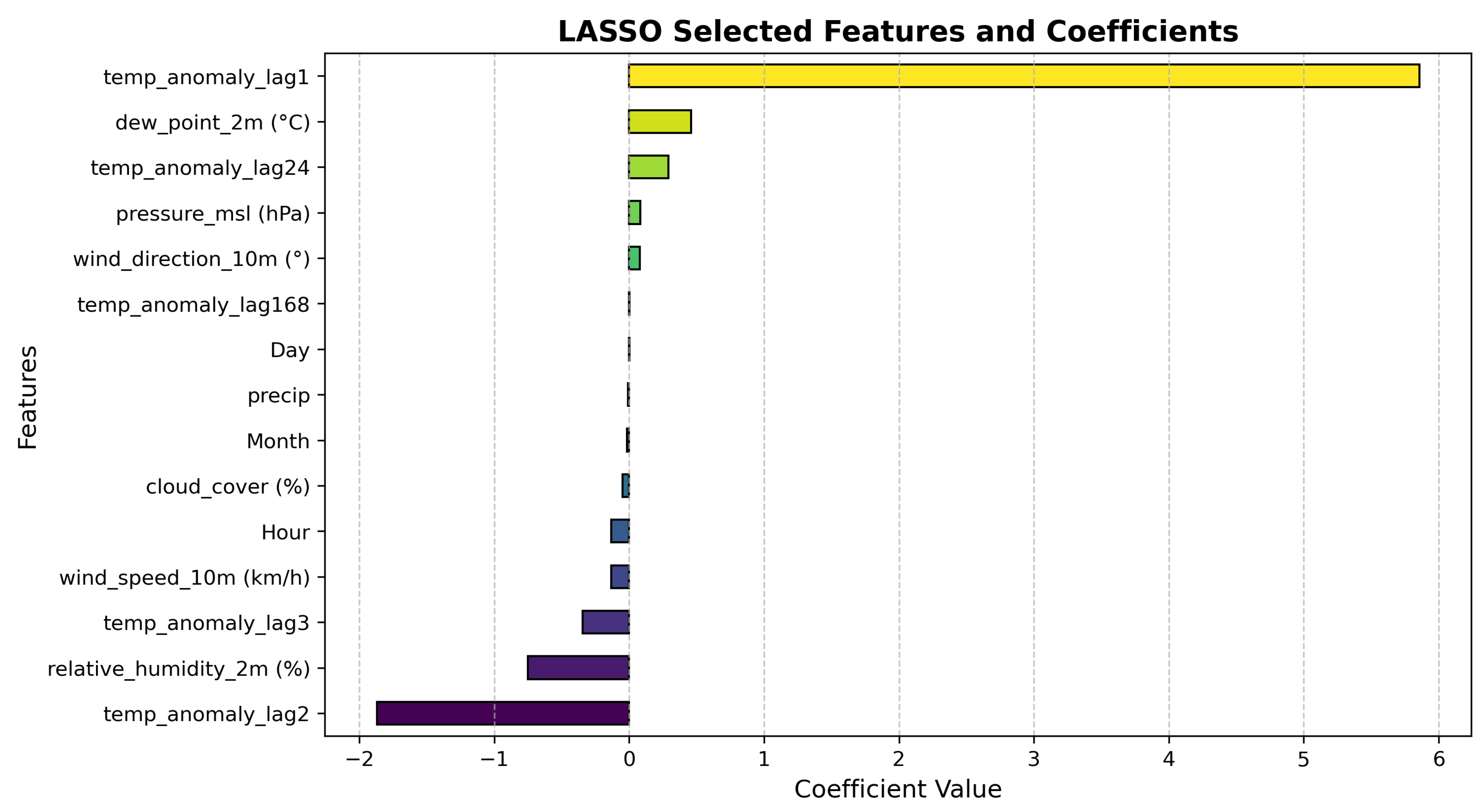
Figure 12.
Feature selection for precipitation anomaly.
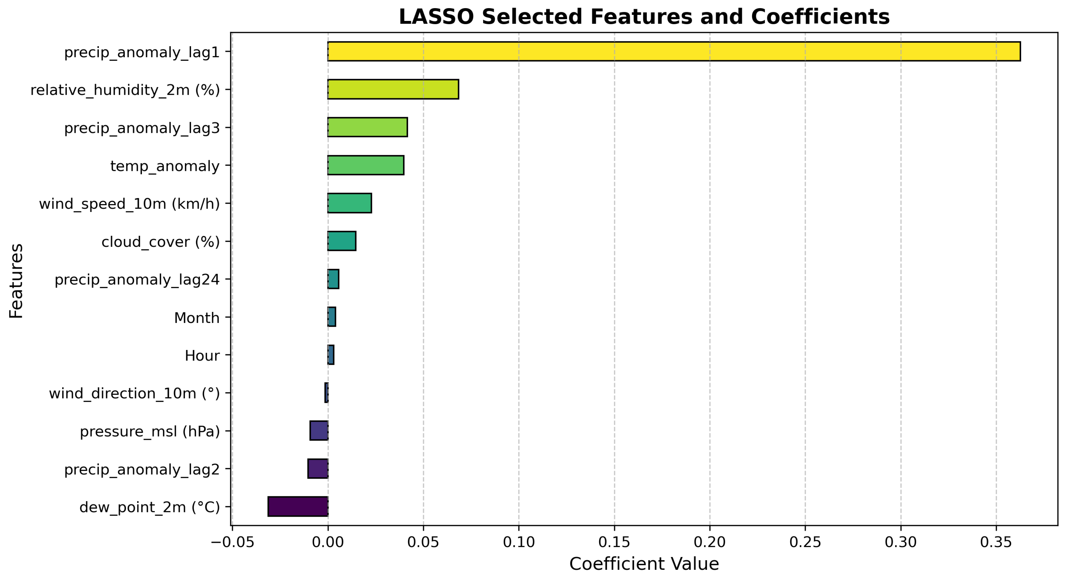
Figure 13.
Comparison of ANN and LSTM predictions with observed temperature anomalies.
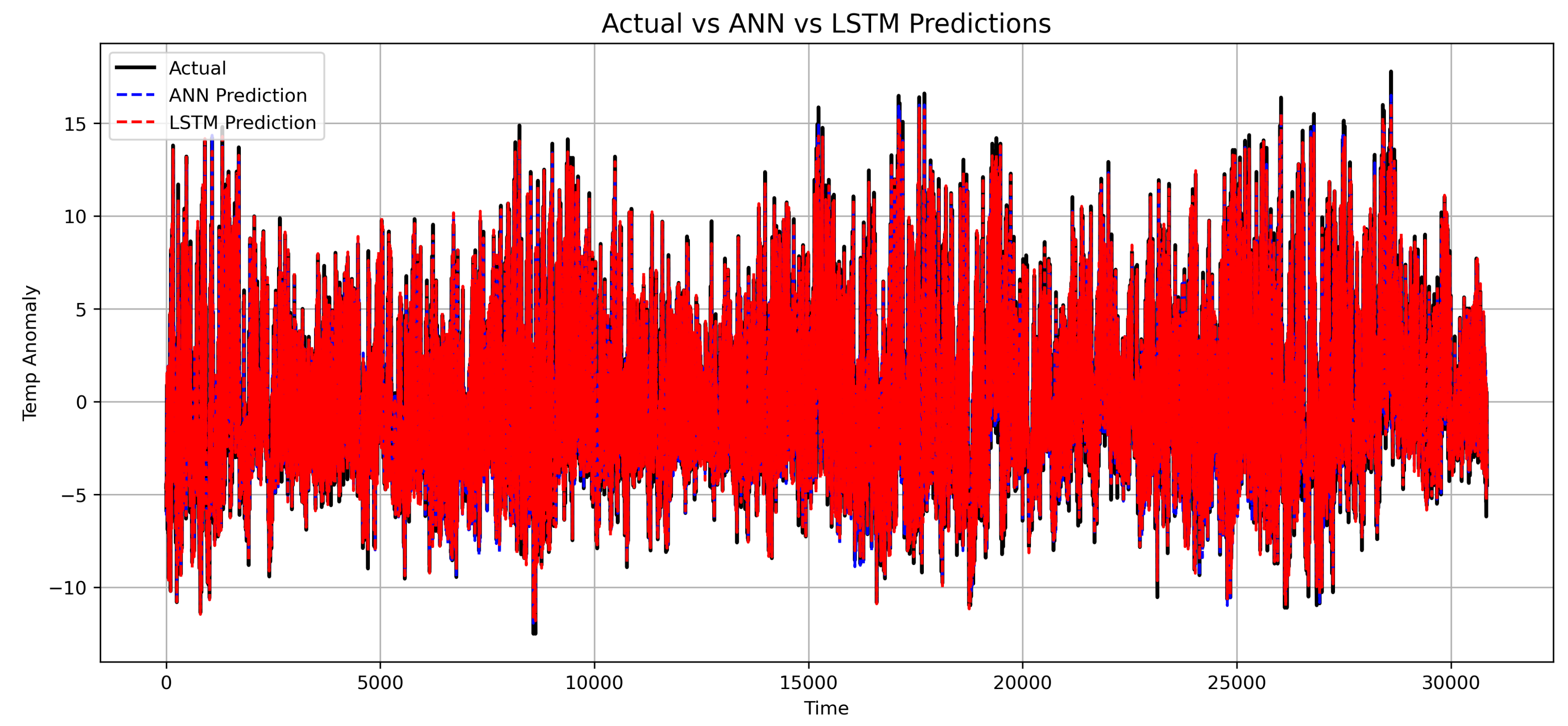
Figure 14.
Zoomed-in view of LSTM predictions compared with observed temperature anomalies.
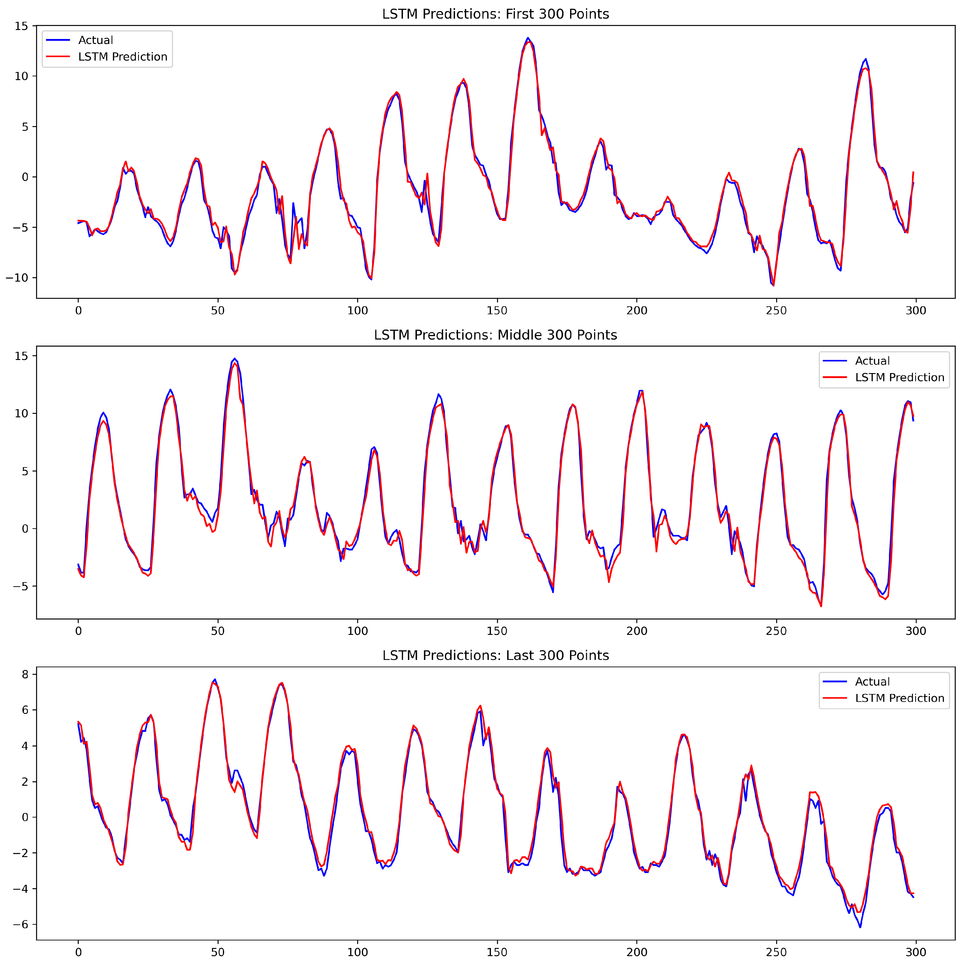
Figure 15.
Comparison of ANN and LSTM predictions with observed precipitation anomalies.
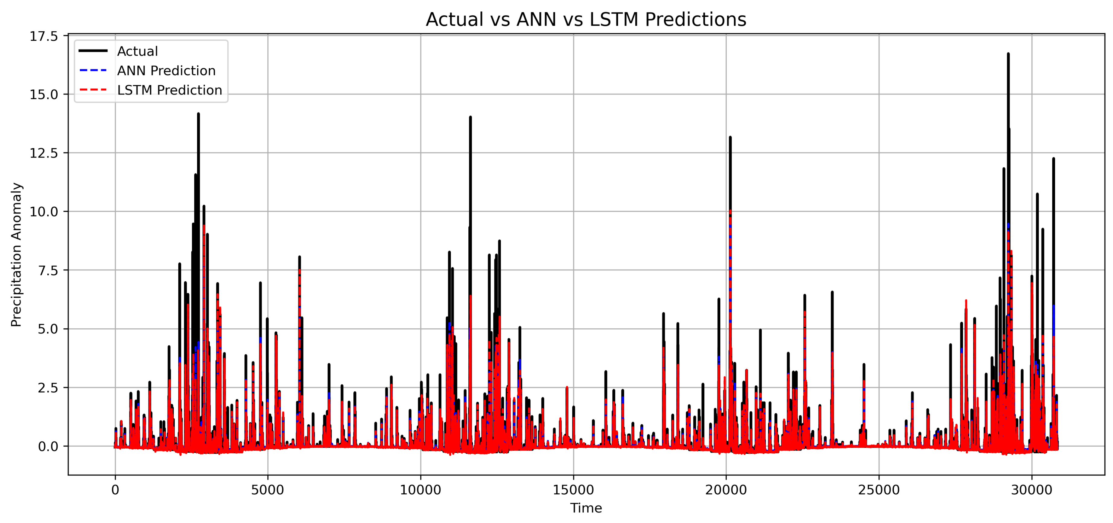
Figure 16.
Zoomed-in view of ANN and LSTM predictions for precipitation anomalies.
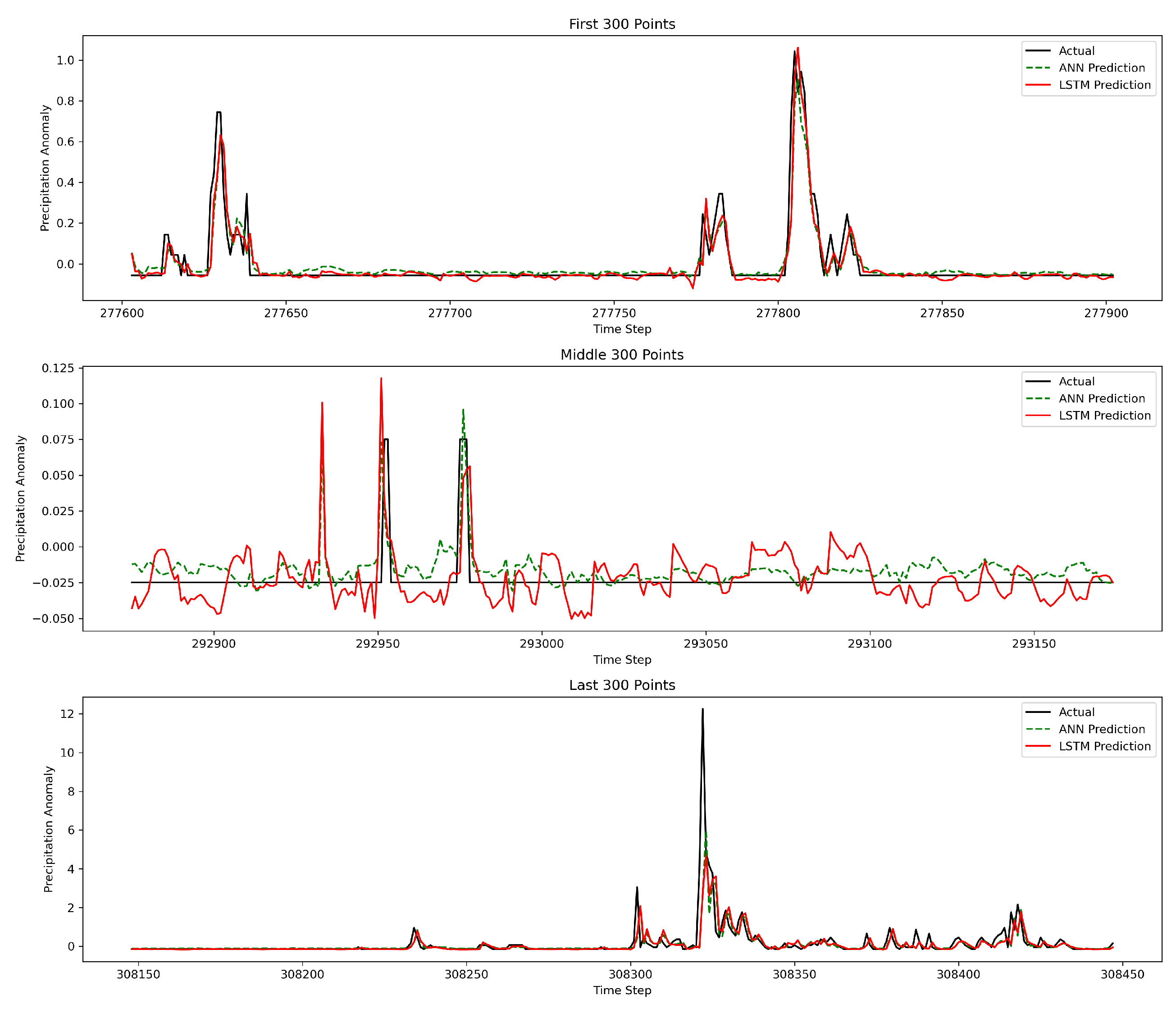

Table 1.
Summary statistics of hourly temperature, precipitation, and anomalies.
| Statistic | temp | precip | temp_anomaly | precip_anomaly |
|---|---|---|---|---|
| Statistic | temp | precip | temp_anomaly | precip_anomaly |
| Count | 308616 | 308616 | 308616 | 308616 |
| Mean | 20.152 | 0.118 | 0.000 | 0.000 |
| Minimum | 4.400 | 0.000 | -12.998 | -0.277 |
| Maximum | 41.300 | 18.600 | 19.938 | 18.341 |
| Std. Deviation | 5.375 | 0.511 | 4.624 | 0.503 |
| Skewness | 0.179 | 10.804 | 0.517 | 10.756 |
| Kurtosis | -0.240 | 186.258 | -0.084 | 188.903 |
Table 2.
Stationarity test results for temperature and precipitation anomalies.
| Variable | Test | Statistic | p-value | Stationary (5%) |
|---|---|---|---|---|
| Temp Anomaly | ADF | -39.154 | 0.000 | Yes |
| Temp Anomaly | KPSS | 1.223 | 0.010 | No |
| Precip Anomaly | ADF | -48.900 | 0.000 | Yes |
| Precip Anomaly | KPSS | 1.438 | 0.010 | No |
Table 3.
BEAST summary results.
| Variable | Change points | Trend slope per year |
|---|---|---|
| Temperature Anomalies | 1992–2020 | 0.0250 |
| Precipitation Anomalies | 1991–2024 | 0.0037 |
Table 4.
Optimal hyperparameters for ANN and LSTM models.
| Target Variable | Model | Batch Size | Epochs | Learning Rate | Units | Dropout Rate |
|---|---|---|---|---|---|---|
| Temperature Anomaly | ANN | 32 | 50 | 0.001 | 64 | 0.2 |
| LSTM | 32 | 50 | 0.001 | 64 | 0.2 | |
| Precipitation Anomaly | ANN | 64 | 50 | 0.001 | 32 | 0.2 |
| LSTM | 64 | 20 | 0.0005 | 32 | 0.2 |
Table 5.
Test set performance of ANN and LSTM models for temperature anomalies.
| Model | RMSE | MAE | MBE | MASE |
|---|---|---|---|---|
| ANN | 0.738 | 0.524 | 0.070 | 0.585 |
| LSTM | 0.678 | 0.466 | 0.123 | 0.520 |
Table 6.
Diebold–Mariano test comparing predictive accuracy of ANN and LSTM models for temperature anomalies.
Table 6.
Diebold–Mariano test comparing predictive accuracy of ANN and LSTM models for temperature anomalies.
| Comparison | DM Statistic | p-value |
|---|---|---|
| ANN vs LSTM | 28.348 | 0.000 |
Table 7.
Test set performance of ANN and LSTM models for precipitation anomalies.
| Model | RMSE | MAE | MBE | MASE |
|---|---|---|---|---|
| ANN | 0.434 | 0.1279 | 0.0097 | 2.1583 |
| LSTM | 0.432 | 0.1124 | -0.0100 | 1.8971 |
Table 8.
Diebold–Mariano test comparing predictive accuracy of ANN and LSTM models for precipitation anomalies.
Table 8.
Diebold–Mariano test comparing predictive accuracy of ANN and LSTM models for precipitation anomalies.
| Comparison | DM Statistic | p-value |
|---|---|---|
| ANN vs LSTM | 0.434 | 0.664 |
Disclaimer/Publisher’s Note: The statements, opinions and data contained in all publications are solely those of the individual author(s) and contributor(s) and not of MDPI and/or the editor(s). MDPI and/or the editor(s) disclaim responsibility for any injury to people or property resulting from any ideas, methods, instructions or products referred to in the content. |
© 2025 by the authors. Licensee MDPI, Basel, Switzerland. This article is an open access article distributed under the terms and conditions of the Creative Commons Attribution (CC BY) license (https://creativecommons.org/licenses/by/4.0/).
Copyright: This open access article is published under a Creative Commons CC BY 4.0 license, which permit the free download, distribution, and reuse, provided that the author and preprint are cited in any reuse.


