Submitted:
06 November 2025
Posted:
07 November 2025
You are already at the latest version
Abstract
Stereo cameras, also known as depth cameras or RGBD cameras, are increasingly employed in a large variety of machinery for obstacle detection purposes and navigation planning. This also represents an opportunity in agricultural machinery for safety purposes to detect the presence of workers on foot and avoid collisions. However, their outdoor performance at medium and long range under operational light conditions remains weakly quantified: authors then fit a field protocol and a model to characterize the pipeline of stereo cameras, taking the Intel RealSense D455 as benchmark, across various distances from 4 meters to 16 meters in realistic farm settings. Tests have been conducted using a 1 square meter planar target in outdoor environments, under diverse illumination conditions and with the panel being located at 0°, 10°, 20° and 35° from the center of the camera's field of view (FoV). Built-in presets were also adjusted during tests, to generate a total of 128 samples. Authors then fit disparity surfaces to predict and correct systematic bias as a function of distance and radial FoV position, allowing to compute mean depth and estimate a model of systematic error that takes depth bias as a function of distance, light conditions and FoV position. Results showed that the model can predict depth errors achieving a good degree of precision in every tested scenario (RMSE: 0.46 – 0.64 m, MAE: 0.40 – 0.51 m), enabling the possibility of replication and benchmarking on other sensors and field contexts while supporting safety-critical perception systems in agriculture.
Keywords:
agriculture
; safety
; RGBD
; depth cameras
; obstacle detection
1. Introduction
Depth perception is one of the key abilities that allow both autonomous and semi-autonomous systems to move safely, plan their paths, and understand their surroundings in most environments, playing a central role in what nowadays is defined as motion planning and obstacle avoidance. Over the past years, compact depth-sensing cameras—often referred to as RGBD or stereo cameras—have become increasingly common thanks to their affordability, small size, and ease of integration [1,2,3]: combining standard color red-green-blue (RGB) images with stereo triangulation, these devices provide real-time depth maps making them useful across a large variety of applications, from mobile robots and logistics to driver-assistance systems and human–robot interaction [4,5].
Although these sensors are now widely used, their reliability in challenging environments is still questionable due to several aspects (weather, light, harsh terrain, etc) and concerns arise when safety systems are solely based on such technology. In fact, most commercial products such as the Intel® RealSense™ D400 series [6], are designed mainly for indoor or short-range robotic use [7,8]. When exposed to outdoor lighting, where brightness can severely change across a sunny day, cloudy conditions and dark environments, their performance naturally tends to drop. This often results in noisy depth data or systematic measurement bias [9,10]. Such limitations are the reason behind safety concerns, particularly in agricultural contexts, where accurate depth information is essential for avoiding collisions and detecting workers on foot [11].
Stereo vision estimates depth by identifying matching points in two or more images taken from slightly different positions and then triangulating their disparities: active stereo cameras expand on this principle by projecting infrared or structured-light patterns, which help find matches even in low-texture areas [12,13]. However, both active and passive systems are vulnerable to strong sunlight, reflections, shadows, and vegetation, all of which can distort the captured patterns and reduce accuracy [14].
A good example is the Intel RealSense D400 series, which uses a global-shutter stereo pair, an optional infrared emitter, and an internal processing pipeline for depth estimation. The camera’s Software Development Kit (SDK) includes several presets—such as Default, High Accuracy, and High Density—that balance precision, range, and data density; however, their performance in outdoor conditions and outside of their standard range remains unpredictable and strongly context-dependent [15]. Prior research has shown, for example, that depth errors tend to increase toward the edges of the field of view [16], and that bright sunlight can amplify noise significantly [17]. Other studies confirm that ambient light and background texture can heavily influence the camera’s effective sensing range [18], also showing how agricultural environments pose some of the toughest challenges for vision-based perception [19,20,21]. Fields and orchards are visually complex, full of dense vegetation, fine textures, and constantly changing lighting conditions [22]. Machinery operating in these environments must also contend with dust, shadows from plants or tools, and oblique sunlight, all of which create strong and unpredictable contrast variations [23]. These factors make it difficult for stereo cameras to maintain stable and accurate depth estimates, especially at medium to long distances (4–15 m), where measurement precision naturally decreases, becoming a crucial factor for autonomous tractors or agricultural robots where reliable detection of people and obstacles is a key safety aspect [24].
Depth cameras are a valid alternative to various sensing technologies that have been explored for agricultural safety: LiDAR sensors offer high accuracy at long ranges but are costly and provide lower resolution [25]; ultrasonic sensors represent a low-cost solution but lack spatial precision, while purely visual systems based on RGB images can recognize humans or obstacles but they do not provide direct depth information [26]. Stereo cameras, therefore, present a promising solution combining good accuracy, coverage, and affordability when their errors can be properly characterized and corrected for real-world conditions.
Recent studies have started to address the need for systematic characterization of stereo cameras in both lab and outdoor settings given the limits of other technologies [27,28]. Moreover, while average error and standard deviation are common evaluation metrics, they do not fully describe how depth bias changes with distance or viewing angle. This is the reason why modeling such source of bias is critical for predicting and correcting systematic errors, as well as for defining reliable confidence bounds that can inform safety-related decisions [29]. In addition, standards such as International Organization for Standardization (ISO) 18497 and ISO 25119 define the performance requirements for systems that operate near humans, emphasizing the importance of measurable and validated sensor reliability [30]; indeed RGBD cameras, despite being highly attractive due to their affordable costs and high-resolution data, are limited by their performance under uncontrolled outdoor environments and in field deployments [31,32].
This work is built on previous research by presenting and validating a field-oriented protocol for testing stereo RGBD cameras in realistic agricultural conditions. Using the Intel RealSense D455 as a case study, a series of controlled outdoor experiments were carried out to examine the effects of three key variables: (i) distance (4–16 m), (ii) field-of-view angle (0°, 10°, 20°, and 35° off-center), and (iii) illumination time. A 1 m2 planar target was used for the tests, placed in vegetation to reflect the visual complexity of contexts such as agriculture and forestry. The goal is to map condition-dependent trade-offs that matter to safety functions, and to provide an error model that can be used to correct raw depth or, at minimum, to inflate safety margins when detection confidence drops.
The protocol deliberately follows the camera’s built-in functions so that the resulting model stays anchored to the physics of stereo vision while remaining practical for field use. Tests have therefore been organized to emphasize the effects of camera presets to obtain a compact and calibrated model that links depth bias to viewing geometry and illumination, which are elements that are directly linked to risk assessment models as well and system configuration settings as countermeasure.
2. Materials and Methods
Starting from the aforementioned state of the art on the use of RGBD cameras for safety purposes, authors selected an Intel RealSense D455 as reference due to its large use in several applications and research studies [33]. Since from a systems engineering perspective understanding how perception uncertainty evolves with lighting and distance would allow adaptive safety margins, authors intended to perform specific tests to evaluate the effects of environmental conditions on visibility and the performances of the sensor at different ranges and angles. As already stated by previous research, distance estimation is affected by an error which might severely limit their applications for safety purposes given the chance of mistakenly assess objects further than away than they effectively are: this is a major issue when safety of vehicles depends on knowing the relative position of obstacles along their trajectory and when the braking distance is higher than the available space, generating the need of a model which is able to provide the error associated with a specific environmental condition and prevent dangerous optimistic estimations.
The research protocol developed for this research follows the camera’s native SDK processing pipeline and evaluates several built-in presets to gather several measurements in different configurations, using a disparity surface to identify and model systematic depth bias as a function of both range and angle of the surface in the Field of View (FoV). The purpose has been to develop a model that could be used either to correct these biases directly or to estimate adaptive safety margins when confidence in sensor data is low, aiming to bridge the gap between controlled laboratory testing and real-world outdoor deployment of stereo cameras. This will contribute to the development of standardized methods for evaluating depth camera’s perception reliability, which is an essential step toward safe and certified use of depth cameras in agricultural machinery.
2.1. Methodology for Depth Error Calibration
To do so, authors designed a research protocol that takes into account both physics and concepts that lay behind the depth estimation methods, starting from how the distance of a pixel is estimated by the camera [34,35] as shown in Figure 1.
The ratio between the distance of the point from the origin (X) and the point’s distance (Z) equals to the ratio of the position of the point in the left image (XL) and focal length (f). Equation 1 shows how XL can therefore be related to focal length and point’s distance:
The same equation can be set up for the position of the point in the right image (XR), but of course the baseline’s length (B) must be subtracted from the X coordinate of the observed point. Equation 2 provides the same information regarding XL for XR as well.
Having obtained XL and XR, disparity (d) can be calculated as the difference among these two values. The result is shown in equation 3:
From that information, distance (Z) can be calculated as follows in equation 4:
This method is used to estimate depth in RGBD cameras starting from a disparity calculated from two optical sensors of known focal length and baseline. To understand how these equations are affected by measurement errors, considerations must be found on derivative estimations on disparity in equation 5.
Equation 5 provides the insights that are required to understand how distance error is generated and what would be required by a model to provide this kind of information. Given that the error is affected by the square of distance and of disparity, with the last being related to the angle at which the pixel is located in the frame, a model that considers these effects has been tested and has been defined as shown in equation 6, with the inclusion of both the assessed distance and the angle of the point plus several calibration weights and their relative interactions.
This model aims to consider a series of parameters that vary according to the situation:
- an offset calibration value (w0) has been considered;
- scale errors (w1) related to the assessed distance;
- the quadratic growth of bias given by noisy measurements (w2Z2);
- a metric related to the field of view’s angle α, in a form (tan α) that aims to adhere to the X/Z ratio used in disparity, with its calibration weight (w3);
- the quadratic growth of bias given by extreme angle measurements, together with its specific weight (w4);
- lastly, overlapping effects of distances and angles again with their weight (w5).
This choice on the mathematical model relies on the will to remain strongly linked to the physics of depth estimations and to leave some flexibility: a greater number of parameters could lead to better results based on test data, but also in overfitting the model to the camera type and field conditions.
2.2. Experimental Design
Tests have been run at the Experimental Farm of Tuscia University located in Viterbo, Italy. Selected area was an environment that is common to many outdoor applications, namely a plain lawn field of approximately 0.15 ha of size. Field layout, including the panel used for tests, is shown in Figure 2.
Having defined the field layout, points have been selected to perform the tests. A set of four points have been selected at distances of 4 m, 8 m, 12 m and 16 m. For each of these points, measurements have been repeated in the following conditions:
- 0 degrees, namely with the camera right in front of the panel. In this condition, the panel will fall exactly in the center of the frame;
- 10° of angle, keeping the camera parallel to the panel, but with it being visible slightly on the right from the center of the frame;
- 20° of angle, with the same camera conditions of the previous scenarios but slightly more toward the edge of the frame;
- 35° of angle, which means that the panel happens nearly on the edge of the frame but is still fully visible at every distance.
The layout of test points is shown in Figure 3.
For each of the 16 test points, a series of camera configurations have been tested, mixing up high-accuracy and high-density mode with its laser emitter enabled or disabled. These are presets available in the Intel RealSense D4xx firmware, where high accuracy aims to provide better results for less pixels while high density tends to provide the highest number of depth estimations in the frame; laser emitter, instead, aims to support depth estimations in the short range to cover poor light conditions. The combinations that have been tested, therefore, are:
- High accuracy mode, laser emitter on;
- High accuracy mode, laser emitter off;
- High density mode, laser emitter on;
- High density mode, laser emitter off.
This experimental configuration leads to 64 diverse tests that had to be performed for each light condition scenario. To cover both good and poor light conditions, these tests have been done on a sunny day in September 2025 at 12:00 PM with approximately 64000 lux of environmental light and on a cloudy day, still in September 2025, approximately at sunset (7:00 PM) with 14000 lux of environmental light. These configurations hence resulted in 128 different tests (16 points, with 4 camera presets and in 2 different scenarios). The acquisition has been performed by making the camera warm up for at least 10 minutes, while in the meantime verifying the proper inclination of the grey panel. As each test started, a .bag file was generated by running a RGB and 2D depth captures for at least 5 seconds from the RealSense Viewer application for Windows 11. Frame resolution was set to 1280x720 pixels for both color and depth frames, each at 30 frames per second of acquisition rate.
2.3. Data Processing and Model Fitting
Data generated by .bag files has been analyzed to identify depth parameters that could be useful for the calibration of the error on each test. The algorithm worked according to this flow of processing:
- Manual selection of the panel area in the frames. A python code reads all the bag files that are found in the folder in which it is located;
- The algorithm processes information such as number of pixels, hole rate of invalid depth values in the panel area, average depth, standard deviation of depth, number of frames and intrinsics;
- A comma separated value (csv) file is generated with all the metrics, alongside with a JSON (JavaScript Object Notation) file that stores data on the bounding boxes that have been defined on the panel area for each .bag file.
After having all the measurements from .bag files into a .csv file, authors processed data to obtain features related to the error of distance compared with ground truth. Given the angle, laser emitter condition, high-accuracy/high-density settings, a Ridge Regression (or Tikhonov regularization) model, provided by the package scikit-learn of Python, has been performed on the aforementioned equation 6 to obtain weights for each scenario. The predicted bias provides corrected depth values according to equation 6 and generated:
- A comparison of errors, for the same environmental and setting conditions, across distances for each test;
- Plots with approximate surfaces of areas sharing the same error according to distance and angle;
- A representation of the raw distance data with ideal condition (ground truth) and with the corrected values generated by the distance error model.
Lastly, data has been saved regarding Root Mean Square Error (RMSE), Mean Squared Error (MAE) and weights of the regression model into another JSON file for subsequent usage in the field. The expected outcome of the tests is to verify error differences among test points and light conditions, with the additional feature of verifying the effect of the presence of laser emitter to support depth readings, resulting in the possibility of analyzing each scenario separately (16 tests for 8 scenarios) or evaluating the possibility of merging the laser emitter on/off scenarios together (32 tests for 4 scenarios) to make a more robust regression model if the effects of laser emitter in open fields are negligible.
3. Results
Results are presented as depth estimations on each of the 128 tests, divided into scenarios, plus the error model estimation based on light conditions, distance and angle.
3.1. Depth Distance Estimations
The outcome of field tests is a wide set of data divided into light conditions, panel angle position and distance from the camera. For each scenario, results are presented for the 4 presets. Tests on depth estimation in daylight with laser off are shown in Table 1, where the data is shown with mean and median distances, standard deviation on the plane surface of the 2D panel, the hole rate and number of valid pixels, which also considers possible abnormal depth values which have been discarded.
Daylight test conditions without laser emitter support showed a progressively greater error as both distances and angle of the panel position in the frame arise. In addition, the percentage of valid pixels (hole rate) changed significantly across high accuracy and high density presets: despite that lowered hole rate values were expected by the high density mode, the number of valid pixels in the plane area around the target in the frames were lower than expected.
Tests have also been run to compare outcomes with laser emitter on and off, in order to evaluate both possible depth assessment improvements and increase of valid pixels. Results of these daylight tests that have been run with laser on are shown in Table 2.
Same tests have been performed at sunset, both with laser emitter off and on as done in daylight conditions. Results are shown in Table 3 and Table 4, where similar patterns observed for daylight have been confirmed in that environmental condition as well.
Distance estimations, as tested in sunset light conditions, started to be less precise as light is reduced; the absence of laser emitter might be responsible for a decrease in precision at close distances but the assessments at far distances started to be significant as the angle of the target panel from the camera increased. It should be noted, however, that even the presence of active laser emitter at maximum power didn’t change the result or improve depth readings, as was already observed in previous daylight tests with laser emitter on. This is shown in the following table, which reports the last run of 32 tests in the given field positions from the target panel. The combination of high accuracy preset, and a reduced presence of external light, played a key role in generating an even lowered percentage of valid pixels in the target area across frames if compared with previous daylight tests.
For each test, further analyses have been done to investigate the influence of laser emitter conditions on depth readings, given that in outdoor environments the effect of this camera enhancement could have been limited. This part of the method is meant to verify if there are significant differences among data and decide whether to perform error regression model estimations separately or not. Results are shown in Table 5, as mean results of the differences of the two corresponding readings for each test point.
No significant differences have been highlighted among the use of the laser emitter in the explored field tests, therefore the upcoming analyses on the precision of the depth sensor at each condition will be explored as datasets of 32 readings (4 distances in 4 angles each) in 4 scenarios which are daylight with high accuracy and high density presets plus sunset scenario with high accuracy and high density presets.
3.2. Distance Error Comparison Among Scenarios
Test data has been compared across scenarios to verify how the error changed as the position of the panel went towards the edge of the frame. An important feature that needed to be assessed was the tendency of the error to vary as the distance of the panel from the camera increased. Results have hence been divided into each one of the 4 scenarios and depth estimation errors are shown in Figure 4.
In each scenario the tendency of the error appears to linearly increase after 8 meters, which is the limit of the expected functionality of the camera model to keep most of the errors below 0.5 or 1 meters; beyond that threshold, errors arise and reach up to 3.5 meters of error in case of poor visibility or far distances, such as 16 meters which is twice the optimal range of the camera.
3.3. Ridge Regression Model for Distance Errors
The 32 tests for each of the 4 scenarios have been employed to run a Ridge regression model to estimate the weights of equation 6. The result of the regression model is shown in Table 6.
From the regression model it is possible to see a high variability between daylight and sunset conditions. More specifically, despite RMSE and MAE remaining stable, the model shows a major impact of the W3 and W4 weights associated with the angle of the panel in the frame. Other parameters, such as W5 associated with variability given by both distance and angle, remain stable within light conditions in both high accuracy and high-density presets.
3.4. Depth Error Estimation Based on Angle and Distance
The depth estimation model has been employed to determine the depth error based on angle and distance from the panel. The error can be represented by a surface on which it remains constant. Figure 5 shows the performance of the model in estimating the error in the 4 scenarios.
The iso-error surfaces in the previous figure show a consistent pattern across scenarios: error, in fact, grows with range as expected but also intensifies as the target moves off-axis, producing steeper contours toward the edges of the FoV. Under daylight conditions, High Density increases spatial coverage (i.e., more usable pixels) but of course it does not prevent angular bias; on the opposite, High Accuracy yields slightly tighter surfaces in the central region while showing comparable off-axis behavior. At sunset light conditions, the angle-driven component becomes more prominent, with wider areas showing higher degree of error confirming that illumination modulates how strongly viewing geometry can generate an impact on depth stability. The plot also provides an intuitive representation of possible safety-critical zones in which the depth correction model can have a greater impact.
To better illustrate how this information can be translated into field use, it can be useful to compare raw depths readings with bias-corrected values from the regression model, as shown in Figure 6.
The compact ridge regression model captured the observed behavior with stable errors across scenarios. Terms linked to viewing angles emerged as especially influential under dimmer light, while interaction terms between range and angle helped explain the rapid growth of bias off axis. The correction attenuates the systematic trend visible in the raw data, especially when overestimation or underestimation accumulates off axis, bringing the observed distances closer to the nominal layout.
4. Discussion
For safety applications on agricultural machinery, the findings have shown in this research translate into concrete design and integration guidance for both autonomous and manned vehicles, with the latter as an alert device or as a tool that provides extra visibility in blind spots. Detection zones that matter for braking and collision avoidance should be placed as close as possible to the optical axis, and system logic should assume larger uncertainty as targets move laterally or fall near the practical range limit. When illumination drops, planners should increase error margins or require other detection methods since the angular component of the error becomes more prominent. Preset selection can be tuned to prioritize coverage when needed, but it will not replace geometry-aware handling of uncertainty. Embedding the proposed bias model in the decision stack allows distance-based rules to operate on corrected values or to adapt thresholds dynamically when conditions predict increased risk of false negatives.
The extremely low outdoor impact of the onboard emitter suggests that, in sunlight and against vegetation, passive stereo remains the dominant mechanism, with limited headroom for active assistance at the tested ranges. This supports a broader strategy that combines model-based correction with operational constraints and, where feasible, fusing complementary sensors to stabilize perception under challenging illumination. It can also be stated that, from a practical point of view, the developed model enables two complementary strategies, namely: apply the corrected distances from obstacles directly in motion planning (i) and alerting or inflating risk thresholds according to the degree of depth measurements’ uncertainty (ii). In both cases, the model can transform static readings driven by fixed presets into a geometry-aware and light-aware depth perception tool.
The limitations of this work are related to the use of a single device class, a controlled yet realistic background, and quasi-static scenes. Studies should, in future, repeat the same scientific protocol to broaden scene diversity, including articulated targets and dynamics to compare across stereo baselines and sensing technologies. Extending the protocol to moving platforms and publishing harmonized datasets would enable fair cross-device benchmarking and help translate model corrections into standardized safety envelopes usable across equipment and environments. Even within these bounds, the proposed approach offers a practical path to quantify, visualize, and mitigate condition-dependent depth errors where it matters most: in the field, under real light, with actionable consequences for machine safety.
5. Conclusions
This study demonstrates that outdoor distance estimation with a stereo RGBD camera is strongly conditioned by where an object sits in the field of view and how the scene is illuminated, with central regions yielding the most stable results and edge placement introducing systematic bias. Camera’s preset selection influences the balance between coverage and precision, yet does not remove the angular dependence of error, while the active projector offers little benefit at typical working ranges. A compact, geometry-informed regression captures these trends and enables bias-aware correction, turning raw depth into distances that align more faithfully with the physical scene.
Taken together, these findings argue for safety pipelines that explicitly manage field-of-view placement, monitor validity density, and apply bias surfaces during risk evaluation rather than treating depth as uniformly reliable across the image. The proposed protocol and modeling workflow are readily transferable, providing a practical basis for acceptance testing, sensor placement, and periodic recalibration in open-air agricultural settings. Embedding these steps into system integration can reduce optimistic distance readings in critical zones and support more dependable human–machine separation, paving the way for standardized, replicable practice across platforms and sites.
Author Contributions
Conceptualization, L.V., D.G. and D.P.; methodology, P.R., E.C., M.C.; software, P.R.; validation, E.C. and D.M.; formal analysis, E.C.; investigation, P.R. and E.C.; resources, E.C. and P.R.; data curation, E.C. and P.R.; writing—original draft preparation, P.R. and E.C.; writing—review and editing, E.C.; visualization, L.V., D.G. and D.P.; supervision, D.M., L.V.; project administration, D.M.; funding acquisition, D.M. All authors have read and agreed to the published version of the manuscript.
Funding
The research is funded by the Italian National Institute for Insurance against Accidents at Work (INAIL) project called “Obstacle detection and tracking system for fixed and moving obstacles in agriculture” (Bando di Ricerca in Collaborazione BRiC 2022 ID04 SIRTRAck).
Institutional Review Board Statement
Not applicable.
Informed Consent Statement
Not applicable.
Data Availability Statement
Raw data (.bag files) from which datasets presented in this study have been derived are available on request due to their size.
Acknowledgments
this research is part of the activities included in “Rome Technopole” Project (ECS 0000024), which is part of the Next Generation EU programme, Italian’s “Piano Nazionale di Ripresa e Resilienza (PNRR)”, mission 4, component 2, investment no. 1.5.
Conflicts of Interest
The authors declare no conflicts of interest.
Abbreviations
The following abbreviations are used in this manuscript:
| FoV | Field of View |
| HA | High Accuracy |
| HD | High Density |
| RGBD | Red, Green, Blue, Depth |
| RMSE | Root Mean Squared Error |
| MAE | Mean Squared Error |
| ISO | International Standard Organization |
| CSV | Comma Separate Values |
| JSON | JavaScript Object Notation |
| 2D | Two dimensions |
References
- R. Hartley and A. Zisserman, Multiple View Geometry in Computer Vision, 2nd ed. Cambridge University Press, 2004. [CrossRef]
- S. Birchfield and C. Tomasi, “Depth Discontinuities by Pixel-to-Pixel Stereo,” Int J Comput Vis, vol. 35, no. 3, pp. 269–293, 1999. [CrossRef]
- F. Rançon et al., “Designing a Proximal Sensing Camera Acquisition System for Vineyard Applications: Results and Feedback on 8 Years of Experiments,” Sensors, vol. 23, no. 2, 2023. [CrossRef]
- J.-M. Park and J.-W. Lee, “Improved Stereo Matching Accuracy Based on Selective Backpropagation and Extended Cost Volume,” Int J Control Autom Syst, vol. 20, pp. 2043–2053, 2022. [CrossRef]
- D. H. C., J. Kannala, and J. Heikkilä, “Joint Depth and Color Camera Calibration with Distortion Correction,” IEEE Trans Pattern Anal Mach Intell, vol. 34, no. 10, pp. 2058–2064, 2012. [CrossRef]
- L. Keselman, J. I. Woodfill, A. Grunnet-Jepsen, and A. Bhowmik, “Intel RealSense Stereoscopic Depth Cameras,” in Proceedings of the IEEE Conference on Computer Vision and Pattern Recognition Workshops (CVPRW), 2017, pp. 1–10. [CrossRef]
- A. Geiger, P. Lenz, and R. Urtasun, “Are We Ready for Autonomous Driving? The KITTI Vision Benchmark Suite,” in Proceedings of the IEEE Conference on Computer Vision and Pattern Recognition (CVPR), 2012, pp. 3354–3361. [CrossRef]
- A. Vit and G. Shani, “Comparing RGB-D Sensors for Close-Range Outdoor Agricultural Phenotyping,” Sensors, vol. 18, no. 12, p. 4413, 2018. [CrossRef]
- S. Birchfield and C. Tomasi, “A Pixel Dissimilarity Measure that is Insensitive to Image Sampling,” IEEE Trans Pattern Anal Mach Intell, vol. 20, no. 4, pp. 401–406, 1998. [CrossRef]
- M. Skoczeń et al., “Obstacle detection system for agricultural mobile robot application using rgb-d cameras,” Sensors, vol. 21, no. 16, Aug. 2021. [CrossRef]
- P. Hübner, J. Hou, and D. Iwaszczuk, “Evaluation of Intel RealSense D455 Camera Depth Estimation for Indoor SLAM Applications,” in The International Archives of the Photogrammetry, Remote Sensing and Spatial Information Sciences, 2023, pp. 1207–1214. [CrossRef]
- M. Servi, A. Profili, R. Furferi, and Y. Volpe, “Comparative Evaluation of Intel RealSense D415, D435i, D455 and Microsoft Azure Kinect DK Sensors for 3D Vision Applications,” IEEE Access, vol. 12, pp. 115919–115932, 2024. [CrossRef]
- A. Upadhyay et al., “Advances in Ground Robotic Technologies for Site-Specific Weed Management in Precision Agriculture: A Review,” Comput Electron Agric, vol. 225, p. 109363, 2024. [CrossRef]
- M. Muñoz-Bañón, F. A. Candelas, and F. Torres, “Targetless Camera–LiDAR Calibration in Unstructured Environments,” IEEE Access, vol. 8, pp. 143692–143705, 2020. [CrossRef]
- G. R. Aby and S. F. Issa, “Safety of Automated Agricultural Machineries: A Systematic Literature Review,” Safety, vol. 9, no. 1, p. 13, 2023. [CrossRef]
- T. Wang, B. Chen, Z. Zhang, H. Li, and M. Zhang, “Applications of Machine Vision in Agricultural Robot Navigation: A Review,” Comput Electron Agric, vol. 198, p. 107085, 2022. [CrossRef]
- P. Kurtser and S. Lowry, “RGB-D Datasets for Robotic Perception in Site-Specific Agricultural Operations – A Survey,” Comput Electron Agric, vol. 212, p. 108035, 2023. [CrossRef]
- M. Camplani and L. Salgado, “Depth–Color Fusion Strategy for 3-D Scene Modeling With Kinect,” IEEE Trans Cybern, vol. 43, no. 6, pp. 1560–1571, 2013. [CrossRef]
- R. Qiu, M. Zhang, and Y. He, “Field estimation of maize plant height at jointing stage using an RGB-D camera,” Crop J, vol. 10, no. 5, pp. 1274–1283, 2022. [CrossRef]
- E. Le Francois et al., “Combining time of flight and photometric stereo imaging for 3D reconstruction of discontinuous scenes,” Opt Lett, vol. 46, no. 15, pp. 3612–3615, 2021. [CrossRef]
- A. Milella, R. Marani, A. Petitti, and G. Reina, “In-field high throughput grapevine phenotyping with a consumer-grade depth camera,” Comput Electron Agric, vol. 156, pp. 293–306, 2019. [CrossRef]
- Ž. Zbontar and Y. LeCun, “Stereo Matching by Training a Convolutional Neural Network to Compare Image Patches,” Journal of Machine Learning Research, vol. 17, pp. 1–32, 2016, [Online]. Available: http://jmlr.org/papers/v17/15-535.html.
- H. Wan, Y. Ou, X. Guan, and others, “Review of the Perception Technologies for Unmanned Agricultural Machinery Operating Environment,” Transactions of the Chinese Society of Agricultural Engineering, vol. 40, no. 8, pp. 1–18, 2024. [CrossRef]
- ”ISO 18497:2018 — Agricultural machinery and tractors — Safety of highly automated agricultural machines — Principles for design,” 2018. [Online]. Available: https://www.iso.org/standard/62659.html.
- M. Carfagni et al., “Metrological and Critical Characterization of the Intel D415 Stereo Depth Camera,” Sensors, vol. 19, no. 3, p. 489, 2019. [CrossRef]
- Y. Qiu and others, “External Multi-Modal Imaging Sensor Calibration: A Review,” Information Fusion, vol. 101, p. 806, 2023. [CrossRef]
- D. Monarca et al., “Autonomous Vehicles Management in Agriculture with Bluetooth Low Energy (BLE) and Passive Radio Frequency Identification (RFID) for Obstacle Avoidance,” Sustainability (Switzerland), vol. 14, no. 15, Aug. 2022. [CrossRef]
- P. Rossi, P. L. Mangiavacchi, D. Monarca, and M. Cecchini, “Smart Machinery and Devices for the Reduction of Risks from Human-machine Interference: a review.”.
- X. Lyu, S. Liu, R. Qiao, S. Jiang, and Y. Wang, “Camera, LiDAR, and IMU Spatiotemporal Calibration: Methodological Review and Research Perspectives,” Sensors, vol. 25, no. 17, p. 5409, 2025. [CrossRef]
- ”ISO 25119 — Tractors and machinery for agriculture and forestry — Safety-related parts of control systems,” 2018. [Online]. Available: https://www.iso.org/standard/69025.html.
- A. Pal, A. C. Leite, and P. J. From, “A Novel End-to-End Vision-Based Architecture for Agricultural Human–Robot Collaboration in Fruit Picking Operations,” Rob Auton Syst, vol. 172, p. 104567, 2024. [CrossRef]
- S. Nebiker and others, “Outdoor Mobile Mapping and AI-Based 3D Object Detection with Low-Cost RGB-D Cameras: The Use Case of On-Street Parking Statistics,” Remote Sens (Basel), vol. 13, no. 16, 2021. [CrossRef]
- P. Gnanamurthy, P. Krishnan, C. Gehlot, and J. Joshi, “Evaluation of Intel® RealSense D455 for 3D Vision Applications,” IEEE Access, 2024, [Online]. Available: https://ieeexplore.ieee.org/.
- M. Kytö, M. Nuutinen, and P. Oittinen, “Method for Measuring Stereo Camera Depth Accuracy Based on Stereoscopic Vision,” in Proc. SPIE Three-Dimensional Imaging, Interaction, and Measurement, 2011. [CrossRef]
- A. Zaremba and others, “Distance Estimation with a Stereo Camera and Accuracy Analysis,” Applied Sciences, vol. 14, no. 23, 2024. [CrossRef]
Figure 1.
Disparity estimation method in depth cameras.
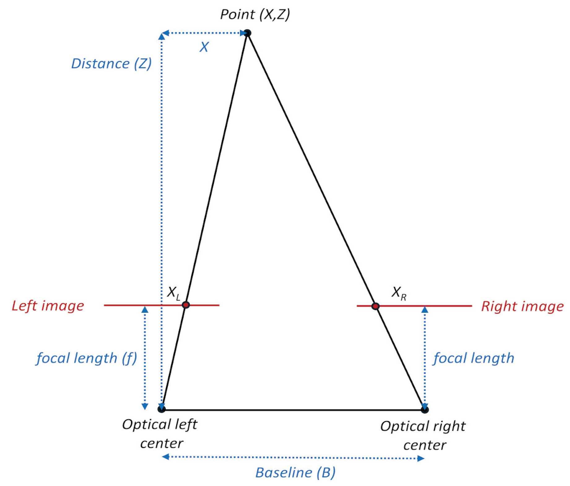
Figure 2.
Field setup for detection tests. Placeholders have been set on the grass as distance reference (a), while the grey panel has been set parallel to the depth camera at each test point (b).
Figure 2.
Field setup for detection tests. Placeholders have been set on the grass as distance reference (a), while the grey panel has been set parallel to the depth camera at each test point (b).
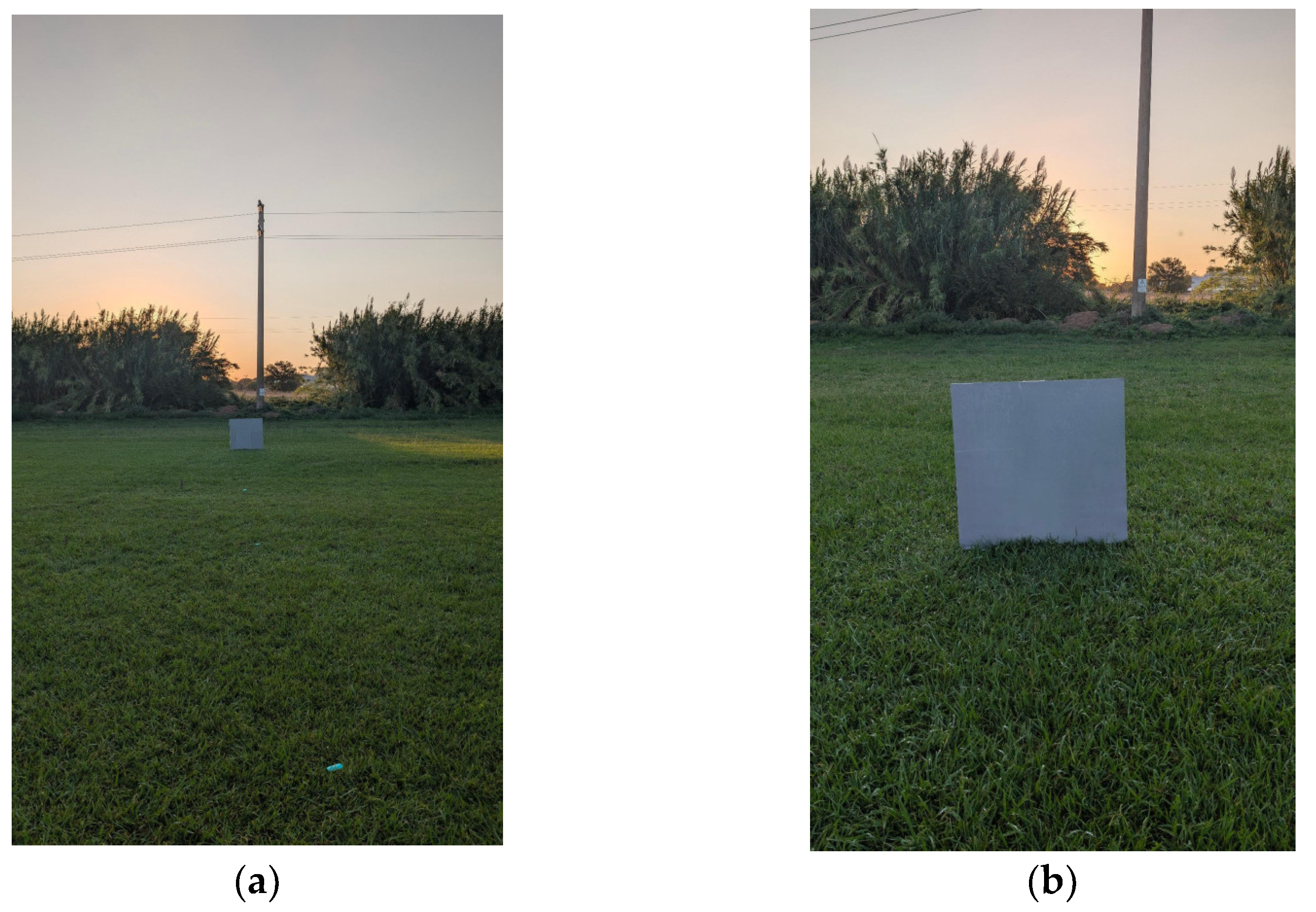
Figure 3.
Test point positions in the map and the criteria used to identify them (b).
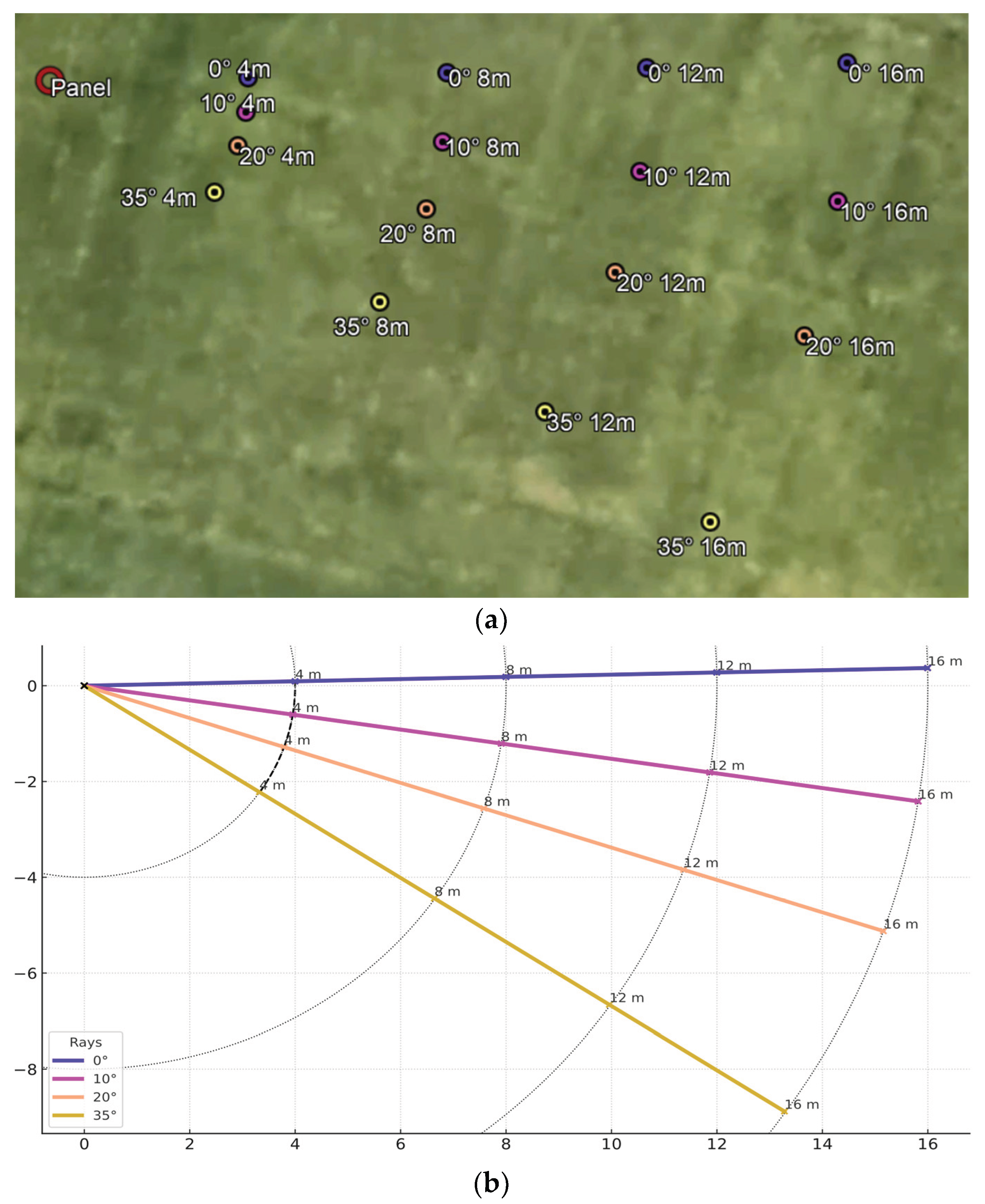
Figure 4.
Error variability in each scenario: daylight and high accuracy preset (a), daylight and high density preset (b), sunset and high accuracy preset (c), sunset and high density preset (d), divided by positioning angle of the panel.
Figure 4.
Error variability in each scenario: daylight and high accuracy preset (a), daylight and high density preset (b), sunset and high accuracy preset (c), sunset and high density preset (d), divided by positioning angle of the panel.

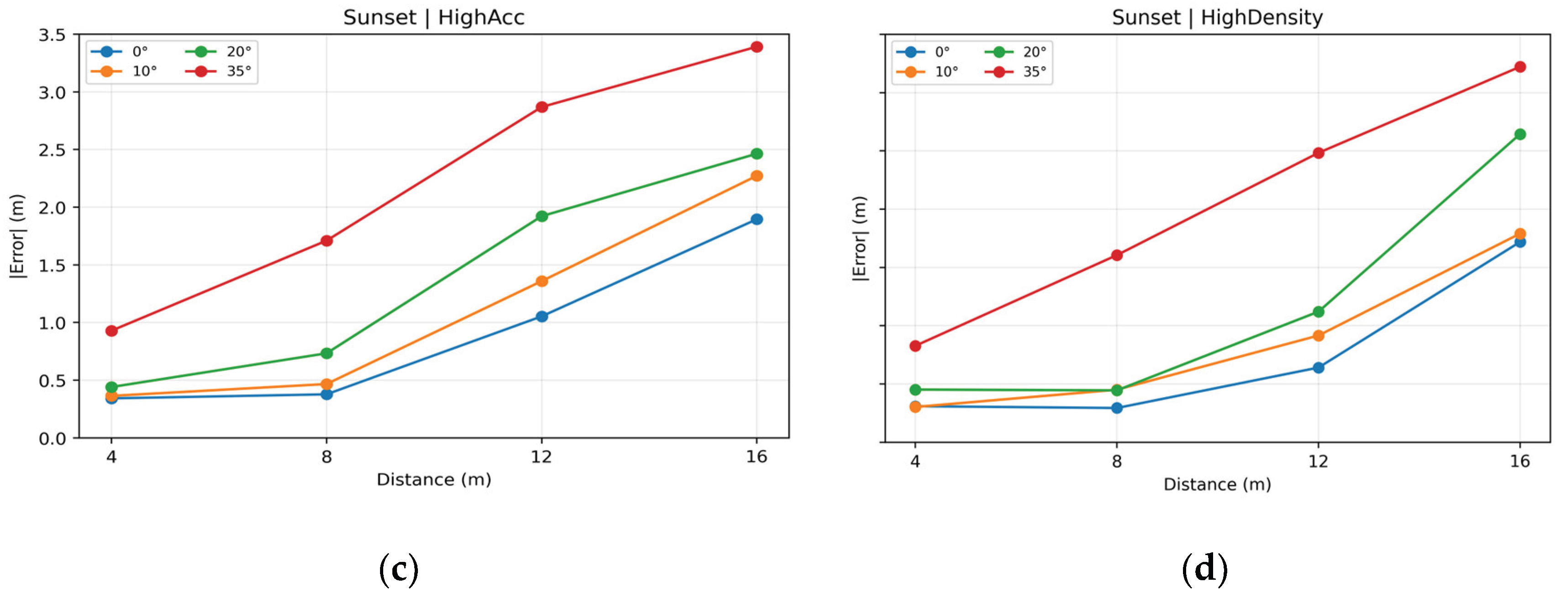
Figure 5.
Depth error estimation according to the regression model for each scenario.
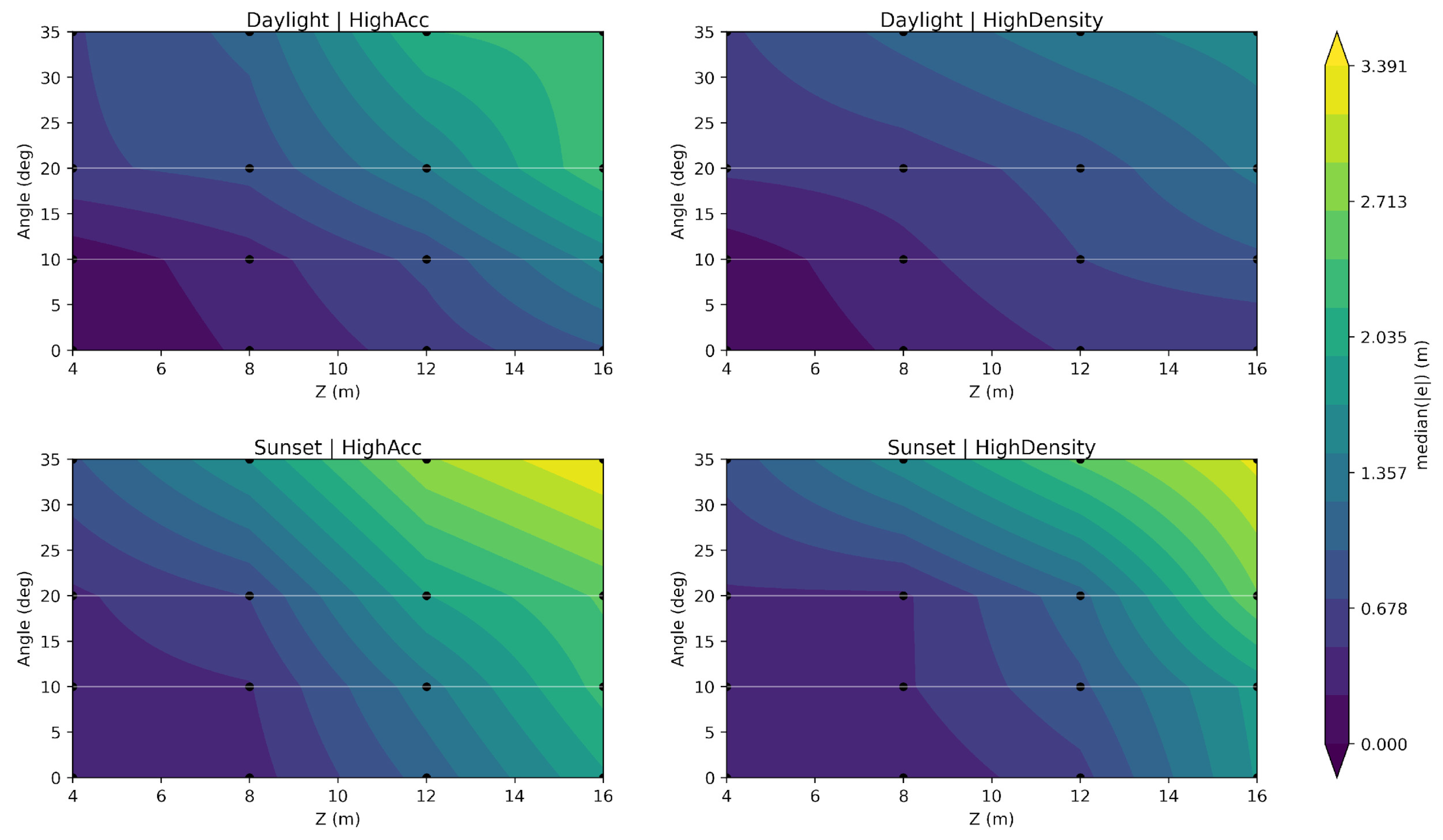
Figure 6.
Comparison among raw depth estimation and model’s correction.
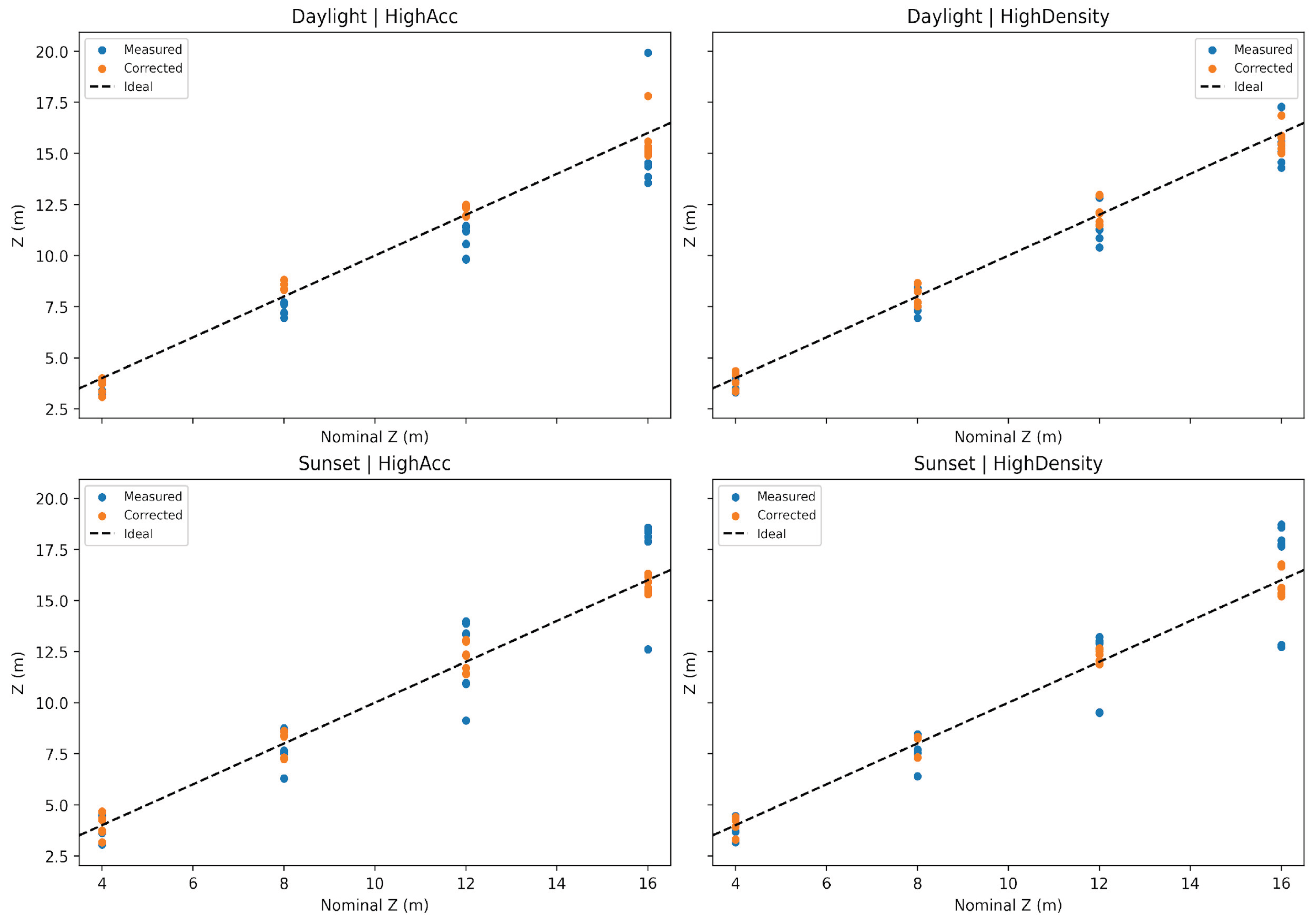

Table 1.
Depth distance results in daylight conditions with laser emitter off. HA and HD stand for High Accuracy and High Density presets.
Table 1.
Depth distance results in daylight conditions with laser emitter off. HA and HD stand for High Accuracy and High Density presets.
| Distance | Position | Preset | Frames | Mean distance | Median distance | Plane std dev | Hole rate | Valid pixels |
| 4 m | 0° | HA | 293 | 3.993 | 3.989 | 0.048 | 37.73% | 62.27% |
| 8 m | 0° | HA | 232 | 7.728 | 7.723 | 0.141 | 35.12% | 64.88% |
| 12 m | 0° | HA | 180 | 11.846 | 11.382 | 0.107 | 67.56% | 32.44% |
| 16 m | 0° | HA | 144 | 16.581 | 15.042 | 0.137 | 55.60% | 44.40% |
| 4 m | 0° | HD | 294 | 4.005 | 3.984 | 0.145 | 6.59% | 93.41% |
| 8 m | 0° | HD | 203 | 7.993 | 7.718 | 0.216 | 11.26% | 88.74% |
| 12 m | 0° | HD | 241 | 13.221 | 11.514 | 0.181 | 9.50% | 90.50% |
| 16 m | 0° | HD | 217 | 17.457 | 15.434 | 0.175 | 3.97% | 96.03% |
| 4 m | 10° | HA | 268 | 3.894 | 3.910 | 0.035 | 95.22% | 4.78% |
| 8 m | 10° | HA | 300 | 7.646 | 7.617 | 0.092 | 66.86% | 33.14% |
| 12 m | 10° | HA | 277 | 11.268 | 11.236 | 0.106 | 61.16% | 38.84% |
| 16 m | 10° | HA | 247 | 14.459 | 14.372 | 0.096 | 47.18% | 52.82% |
| 4 m | 10° | HD | 291 | 4.374 | 3.909 | 0.169 | 75.43% | 24.57% |
| 8 m | 10° | HD | 283 | 9.472 | 8.426 | 0.170 | 37.61% | 62.39% |
| 12 m | 10° | HD | 271 | 11.609 | 11.296 | 0.153 | 10.32% | 89.68% |
| 16 m | 10° | HD | 219 | 17.843 | 15.088 | 0.152 | 5.91% | 94.09% |
| 4 m | 20° | HA | 300 | 3.205 | 3.231 | 0.018 | 99.57% | 0.43% |
| 8 m | 20° | HA | 300 | 7.189 | 7.221 | 0.031 | 96.62% | 3.38% |
| 12 m | 20° | HA | 300 | 10.573 | 10.573 | 0.038 | 94.48% | 5.52% |
| 16 m | 20° | HA | 276 | 15.137 | 15.136 | 0.044 | 94.00% | 6.00% |
| 4 m | 20° | HD | 300 | 3.837 | 3.459 | 0.180 | 81.74% | 18.26% |
| 8 m | 20° | HD | 300 | 8.405 | 7.314 | 0.144 | 62.13% | 37.87% |
| 12 m | 20° | HD | 295 | 14.982 | 12.826 | 0.153 | 41.37% | 58.63% |
| 16 m | 20° | HD | 300 | 19.256 | 17.286 | 0.128 | 37.36% | 62.64% |
| 4 m | 35° | HA | 195 | 3.304 | 3.296 | 0.047 | 72.84% | 27.16% |
| 8 m | 35° | HA | 206 | 6.955 | 6.957 | 0.117 | 34.66% | 65.34% |
| 12 m | 35° | HA | 290 | 9.897 | 9.812 | 0.066 | 85.28% | 14.72% |
| 16 m | 35° | HA | 300 | 14.001 | 13.856 | 0.044 | 90.80% | 9.20% |
| 4 m | 35° | HD | 239 | 3.354 | 3.311 | 0.169 | 37.96% | 62.04% |
| 8 m | 35° | HD | 300 | 7.002 | 6.951 | 0.173 | 7.38% | 92.62% |
| 12 m | 35° | HD | 300 | 14.932 | 10.862 | 0.228 | 34.80% | 65.20% |
| 16 m | 35° | HD | 289 | 14.345 | 14.294 | 0.181 | 20.99% | 79.01% |
Table 2.
Depth distance results in daylight conditions with laser emitter on.
| Distance | Position | Preset | Frames | Mean distance | Median distance | Plane std dev | Hole rate | Valid pixels |
| 4 m | 0° | HA | 300 | 3.994 | 3.990 | 0.049 | 38.05% | 61.95% |
| 8 m | 0° | HA | 184 | 7.717 | 7.715 | 0.144 | 36.01% | 63.99% |
| 12 m | 0° | HA | 195 | 11.524 | 11.454 | 0.136 | 39.91% | 60.09% |
| 16 m | 0° | HA | 206 | 15.818 | 15.078 | 0.140 | 54.81% | 45.19% |
| 4 m | 0° | HD | 249 | 4.052 | 3.983 | 0.242 | 7.41% | 92.59% |
| 8 m | 0° | HD | 191 | 7.900 | 7.714 | 0.212 | 8.60% | 91.40% |
| 12 m | 0° | HD | 169 | 13.130 | 11.457 | 0.194 | 7.89% | 92.11% |
| 16 m | 0° | HD | 175 | 17.700 | 15.555 | 0.169 | 4.11% | 95.89% |
| 4 m | 10° | HA | 234 | 3.897 | 3.914 | 0.039 | 95.28% | 4.72% |
| 8 m | 10° | HA | 263 | 7.650 | 7.611 | 0.100 | 60.93% | 39.07% |
| 12 m | 10° | HA | 212 | 11.165 | 11.175 | 0.100 | 57.42% | 42.58% |
| 16 m | 10° | HA | 249 | 14.774 | 14.528 | 0.108 | 53.11% | 46.89% |
| 4 m | 10° | HD | 300 | 4.550 | 3.908 | 0.174 | 75.61% | 24.39% |
| 8 m | 10° | HD | 276 | 8.654 | 8.419 | 0.172 | 44.14% | 55.86% |
| 12 m | 10° | HD | 271 | 11.519 | 11.261 | 0.155 | 9.84% | 90.16% |
| 16 m | 10° | HD | 212 | 17.850 | 15.059 | 0.148 | 6.19% | 93.81% |
| 4 m | 20° | HA | 300 | 3.324 | 3.402 | 0.023 | 99.02% | 0.98% |
| 8 m | 20° | HA | 272 | 7.151 | 7.165 | 0.028 | 97.43% | 2.57% |
| 12 m | 20° | HA | 270 | 10.517 | 10.554 | 0.037 | 92.45% | 7.55% |
| 16 m | 20° | HA | 262 | 20.547 | 19.924 | 0.078 | 94.55% | 5.45% |
| 4 m | 20° | HD | 300 | 3.896 | 3.484 | 0.177 | 82.26% | 17.74% |
| 8 m | 20° | HD | 300 | 8.822 | 7.499 | 0.149 | 62.61% | 37.39% |
| 12 m | 20° | HD | 300 | 13.596 | 12.846 | 0.137 | 40.50% | 59.50% |
| 16 m | 20° | HD | 281 | 19.235 | 17.265 | 0.144 | 33.75% | 66.25% |
| 4 m | 35° | HA | 187 | 3.308 | 3.300 | 0.046 | 74.05% | 25.95% |
| 8 m | 35° | HA | 300 | 6.957 | 6.954 | 0.112 | 37.24% | 62.76% |
| 12 m | 35° | HA | 266 | 9.887 | 9.845 | 0.101 | 70.29% | 29.71% |
| 16 m | 35° | HA | 300 | 13.958 | 13.561 | 0.050 | 89.93% | 10.07% |
| 4 m | 35° | HD | 208 | 3.353 | 3.308 | 0.171 | 40.76% | 59.24% |
| 8 m | 35° | HD | 271 | 6.983 | 6.957 | 0.170 | 6.86% | 93.14% |
| 12 m | 35° | HD | 300 | 13.397 | 10.390 | 0.207 | 36.50% | 63.50% |
| 16 m | 35° | HD | 300 | 14.873 | 14.565 | 0.187 | 19.34% | 80.66% |
Table 3.
Depth distance results in sunset conditions with laser emitter off.
| Distance | Position | Preset | Frames | Mean distance | Median distance | Plane std dev | Hole rate | Valid pixels |
| 4 m | 0° | HA | 300 | 3.664 | 3.667 | 0.037 | 99.32% | 0.68% |
| 8 m | 0° | HA | 300 | 7.692 | 7.583 | 0.036 | 98.46% | 1.54% |
| 12 m | 0° | HA | 300 | 10.990 | 10.913 | 0.048 | 95.16% | 4.84% |
| 16 m | 0° | HA | 300 | 17.890 | 17.905 | 0.057 | 91.38% | 8.62% |
| 4 m | 0° | HD | 300 | 3.728 | 3.695 | 0.205 | 68.40% | 31.60% |
| 8 m | 0° | HD | 300 | 8.312 | 7.711 | 0.203 | 39.59% | 60.41% |
| 12 m | 0° | HD | 300 | 13.932 | 12.642 | 0.197 | 28.96% | 71.04% |
| 16 m | 0° | HD | 300 | 17.632 | 17.754 | 0.186 | 18.25% | 81.75% |
| 4 m | 10° | HA | 300 | 3.627 | 3.639 | 0.026 | 98.41% | 1.59% |
| 8 m | 10° | HA | 274 | 7.509 | 7.489 | 0.029 | 97.77% | 2.23% |
| 12 m | 10° | HA | 281 | 13.398 | 13.393 | 0.039 | 98.55% | 1.45% |
| 16 m | 10° | HA | 300 | 18.516 | 18.425 | 0.048 | 98.12% | 1.88% |
| 4 m | 10° | HD | 300 | 3.900 | 3.696 | 0.202 | 53.95% | 46.05% |
| 8 m | 10° | HD | 300 | 8.649 | 7.564 | 0.167 | 50.61% | 49.39% |
| 12 m | 10° | HD | 277 | 12.849 | 12.903 | 0.180 | 47.36% | 52.64% |
| 16 m | 10° | HD | 300 | 18.761 | 17.936 | 0.192 | 29.15% | 70.85% |
| 4 m | 20° | HA | 233 | 4.502 | 4.464 | 0.065 | 97.94% | 2.06% |
| 8 m | 20° | HA | 300 | 8.720 | 8.713 | 0.031 | 97.44% | 2.56% |
| 12 m | 20° | HA | 300 | 13.078 | 13.979 | 0.019 | 99.59% | 0.41% |
| 16 m | 20° | HA | 300 | 18.392 | 18.353 | 0.074 | 99.16% | 0.84% |
| 4 m | 20° | HD | 298 | 4.535 | 4.451 | 0.204 | 51.85% | 48.15% |
| 8 m | 20° | HD | 300 | 8.551 | 8.457 | 0.175 | 44.95% | 55.05% |
| 12 m | 20° | HD | 300 | 16.312 | 13.217 | 0.190 | 26.07% | 73.94% |
| 16 m | 20° | HD | 251 | 18.578 | 18.575 | 0.142 | 22.44% | 77.56% |
| 4 m | 35° | HA | 300 | 3.067 | 3.046 | 0.017 | 96.41% | 3.59% |
| 8 m | 35° | HA | 283 | 6.295 | 6.296 | 0.065 | 89.21% | 10.79% |
| 12 m | 35° | HA | 300 | 9.123 | 9.131 | 0.037 | 90.83% | 9.17% |
| 16 m | 35° | HA | 282 | 12.588 | 12.605 | 0.061 | 76.99% | 23.01% |
| 4 m | 35° | HD | 300 | 3.193 | 3.170 | 0.108 | 44.66% | 55.34% |
| 8 m | 35° | HD | 300 | 6.548 | 6.391 | 0.155 | 22.65% | 77.35% |
| 12 m | 35° | HD | 300 | 10.816 | 9.505 | 0.163 | 38.71% | 61.29% |
| 16 m | 35° | HD | 300 | 12.679 | 12.839 | 0.139 | 7.78% | 92.22% |
Table 4.
Depth distance results in sunset conditions with laser emitter on.
| Distance | Position | Preset | Frames | Mean distance | Median distance | Plane std dev | Hole rate | Valid pixels |
| 4 m | 0° | HA | 300 | 3.644 | 3.647 | 0.035 | 99.26% | 0.74% |
| 8 m | 0° | HA | 300 | 7.674 | 7.661 | 0.051 | 97.96% | 2.04% |
| 12 m | 0° | HA | 300 | 11.038 | 10.979 | 0.047 | 94.92% | 5.08% |
| 16 m | 0° | HA | 300 | 17.945 | 17.887 | 0.052 | 95.22% | 4.78% |
| 4 m | 0° | HD | 300 | 3.710 | 3.686 | 0.210 | 68.47% | 31.53% |
| 8 m | 0° | HD | 300 | 8.691 | 7.701 | 0.213 | 40.24% | 59.76% |
| 12 m | 0° | HD | 300 | 13.721 | 12.641 | 0.192 | 28.38% | 71.62% |
| 16 m | 0° | HD | 300 | 17.588 | 17.684 | 0.180 | 16.49% | 83.51% |
| 4 m | 10° | HA | 298 | 3.633 | 3.632 | 0.037 | 97.55% | 2.45% |
| 8 m | 10° | HA | 300 | 7.707 | 7.577 | 0.035 | 97.00% | 3.00% |
| 12 m | 10° | HA | 300 | 13.348 | 13.326 | 0.030 | 98.81% | 1.19% |
| 16 m | 10° | HA | 300 | 18.252 | 18.120 | 0.054 | 95.82% | 4.18% |
| 4 m | 10° | HD | 300 | 3.897 | 3.698 | 0.205 | 54.77% | 45.23% |
| 8 m | 10° | HD | 300 | 8.696 | 7.533 | 0.168 | 52.84% | 47.16% |
| 12 m | 10° | HD | 291 | 12.812 | 12.930 | 0.161 | 45.28% | 54.72% |
| 16 m | 10° | HD | 300 | 18.843 | 17.645 | 0.182 | 29.03% | 70.97% |
| 4 m | 20° | HA | 300 | 4.539 | 4.419 | 0.033 | 98.11% | 1.89% |
| 8 m | 20° | HA | 300 | 8.965 | 8.754 | 0.036 | 97.44% | 2.56% |
| 12 m | 20° | HA | 284 | 13.895 | 13.866 | 0.035 | 99.46% | 0.54% |
| 16 m | 20° | HA | 223 | 18.469 | 18.575 | 0.097 | 99.11% | 0.89% |
| 4 m | 20° | HD | 267 | 4.515 | 4.454 | 0.204 | 52.25% | 47.75% |
| 8 m | 20° | HD | 300 | 8.435 | 8.434 | 0.172 | 44.56% | 55.44% |
| 12 m | 20° | HD | 280 | 15.576 | 13.025 | 0.182 | 27.50% | 72.50% |
| 16 m | 20° | HD | 300 | 18.986 | 18.715 | 0.156 | 22.07% | 77.93% |
| 4 m | 35° | HA | 300 | 3.098 | 3.095 | 0.015 | 97.52% | 2.48% |
| 8 m | 35° | HA | 300 | 6.282 | 6.283 | 0.063 | 90.69% | 9.31% |
| 12 m | 35° | HA | 300 | 9.119 | 9.132 | 0.030 | 91.73% | 8.27% |
| 16 m | 35° | HA | 279 | 12.613 | 12.612 | 0.062 | 77.38% | 22.62% |
| 4 m | 35° | HD | 300 | 3.192 | 3.174 | 0.109 | 46.96% | 53.04% |
| 8 m | 35° | HD | 296 | 6.698 | 6.397 | 0.157 | 23.54% | 76.46% |
| 12 m | 35° | HD | 265 | 10.843 | 9.528 | 0.150 | 40.99% | 59.01% |
| 16 m | 35° | HD | 296 | 12.690 | 12.718 | 0.149 | 8.80% | 91.20% |
Table 5.
Mean difference of measurements among light conditions for laser emitter on and off.
|
Light condition |
Δ distance (mean) | Δ distance (median) | Δ plane std dev | Δ hole rate | Δ valid pixels |
| Daylight | -0.060 | -0.151 | -0.007 | 0.013 | -0.013 |
| Sunset | -0.034 | 0.018 | 0.000 | -0.003 | 0.003 |
Table 6.
Weights and regression errors for each scenario.
| Light | Preset | Wo | W1 | W2 | W3 | W4 | W5 | RMSE | MAE |
| Daylight | HA | 2.543 | -0.714 | 0.035 | -0.837 | -1.630 | 0.054 | 0.635 | 0.509 |
| HD | 0.484 | -0.217 | 0.010 | 2.606 | -5.857 | 0.054 | 0.541 | 0.459 | |
| Sunset | HA | -0.493 | -0.211 | 0.019 | 12.683 | -17.073 | -0.358 | 0.550 | 0.491 |
| HD | -0.278 | -0.179 | 0.017 | 9.834 | -13.237 | -0.358 | 0.461 | 0.401 |
Disclaimer/Publisher’s Note: The statements, opinions and data contained in all publications are solely those of the individual author(s) and contributor(s) and not of MDPI and/or the editor(s). MDPI and/or the editor(s) disclaim responsibility for any injury to people or property resulting from any ideas, methods, instructions or products referred to in the content. |
© 2025 by the authors. Licensee MDPI, Basel, Switzerland. This article is an open access article distributed under the terms and conditions of the Creative Commons Attribution (CC BY) license (http://creativecommons.org/licenses/by/4.0/).
Copyright: This open access article is published under a Creative Commons CC BY 4.0 license, which permit the free download, distribution, and reuse, provided that the author and preprint are cited in any reuse.


