Comparative Analysis of Convolutional Neural Networks for Optical Fiber Classification

1. Introduction

Industrialization and technological advances incite the development of new applications in infrastructure and telecommunications. The latter makes use of several ways of transmission, namely satellite communications, radio waves, 4G, 5G (through air), coaxial cables, RJ-45 cables, and optical fibers. Optical fibers, in their turn, are utilized because of their characteristics such as natural immunity to electromagnetic interference (EMI), dielectric conductivity, low loss of data, and high transmission rates (close to light speed).

Although optical fiber guides are quite fragile. Despite all their shields and protections, varying according to the installation type (aerial, underwater, directly underground, or through ducts), optical fiber cables are not immune to mechanical failure that can compromise, entirely or partly, their transmission capacity [1]. Despite going under a rigid quality control from the suppliers, optical fibers end up, sometimes, being wrongly installed and thus are prone to environmental stress wherever they are set. This results in a reduced lifespan, which can rapidly compromise their characteristics.

Initial studies of the application of image processing for optical fiber were done in our previous research work [2]. So, the purpose of this work is to improve upon a solution for an industry problem that may be free of any operator influence. This will be done through an automation of the quality verification on optical fiber cables regarding the micro-curvatures problem that can occur on optical fiber light guides due to improper handling or installation. The main contributions of this work are: 1) Using image processing for optical fiber classification; 2) Application of deep learning to the problem of optical fiber classification; 3) Implementing the data augmentation technique for an optical fiber dataset; 4) Comparison of two different kinds of neural networks for optical fiber classification. Another contribution is making available for anyone the dataset of optical fiber images of this article [3].

This paper is divided into six sections. After a brief introduction, the second section relates some previous works developed, the third section explains the main techniques used, the fourth section describes the materials and methods employed, the results are presented in the fifth section, and finally, the conclusions are summarized in the last section.

2. Related Work

Based on a review of the literature, this is among the first studies using image processing to find optical fiber flaws. Visually observing the fiber from a transverse viewpoint, Shahrara, Schmidt, and Palmquist [1] closely related study on defect detection, classification, and quantification in optical fiber connectors investigates. Research by Sinha and Fieguth [4] on the automatic inspection of underground ducts, where an image recognition technique for inspection is developed, provides notable references regarding the application of image processing for defect detection in various materials, such as tubes or ducts. Using graphical analysis of the fiber’s specular pattern, Hägele [5] developed an application that finds the curvature angle of the fiber. An edge detection technique allows one to clearly see the outlines of the speckles in a specified area of the specular pattern; their quantity is adjusted in line with the angle of curvature.

Investigating an optical fiber parameter measuring technique, the authors in [6] show a comparison between a developed method and a traditional optical fiber measurement technique. Research on a technique allowing radiographic images of pipes and welding to automatically segment flaws also exists.

Optical fiber has also been applied for the design of new sensors, such as the work by [7] that has used an optical fiber polymer for the design of torque and curvature measurement sensors. The authors in [8] have employed optical fiber sensors to construct a Bragg grating sensor network that is implanted in an insole that is adapted to a shoe. Other applications of optical fiber used for sensors could be found in the works where the optical fiber is used as a strain gauge [9], as a temperature sensor [10], and as a liquid level measurement sensor [11]. Another application is the use of the polymeric optical fiber sensor for applications of measurement of cardiac frequency and breathing [12].

Convolutional neural networks (CNN) have been applied to identify problems based on image classification; in [13], AlexNet, GoogleNet, VGG-16, and ResNet50 are applied for identifying defects in x-ray pipe images. In [14], the VGG-16 and ResNet neural networks were used for chest x-ray image segmentation and binary classification of normal vs. pneumonia-annotated images.

Shin in [15] used 3 different neural architectures—AlexNet, CifarNet, and GoogleNet—for the detection of two different kinds of pulmonary diseases through x-ray analysis; the tests were made using two different datasets. Lv et al. in [16] used AlexNet, VGG-16 and ResNet-50 and added information derived from the SIFT and RootSIFT feature detectors, proposing a technique named complementary supervision mining for learning more specific characteristics in the models. Yun in [17] used SE-ResNet, a modified ResNet with a Squeeze and Excitation block (SE), to detect breast cancer. Kaur and Gandhi in [18] used the VGG-16 for a dataset of image resonance images of neurological diseases.

Ramzan in [19] also used a dataset of resonance images and employed ResNet-18 to classify patterns for Alzheimer’s disease at different levels of advancement of the disease. Mikołajczyk and Grochowski in [20] used a VGG16 in three different medicine datasets and also compared different data augmentation techniques. As far as we know, this is one of the few works that applies artificial intelligence methods using image processing to classify optical fiber, continuing our initial research work that used fuzzy logic [2].

3. Theoretical Background

3.1. Optical Fiber

Optical fiber is a cylindrical guide that carries electromagnetic energy in the form of light within its surfaces. Due to their structural characteristics, optical fibers have the transmission properties of an optical waveguide [21]. An optical fiber consists of a tube with several layers of glass in concentric rings. The light signal is transmitted and reflected from the walls inside the fiber. Each layer (or ring) of glass has a different refractive index n. Figure 1 shows an optical fiber with its main components, such as the core, the shell, and the acrylate coating

Figure 1. Optical Fiber structure

Figure 1. Optical Fiber structure

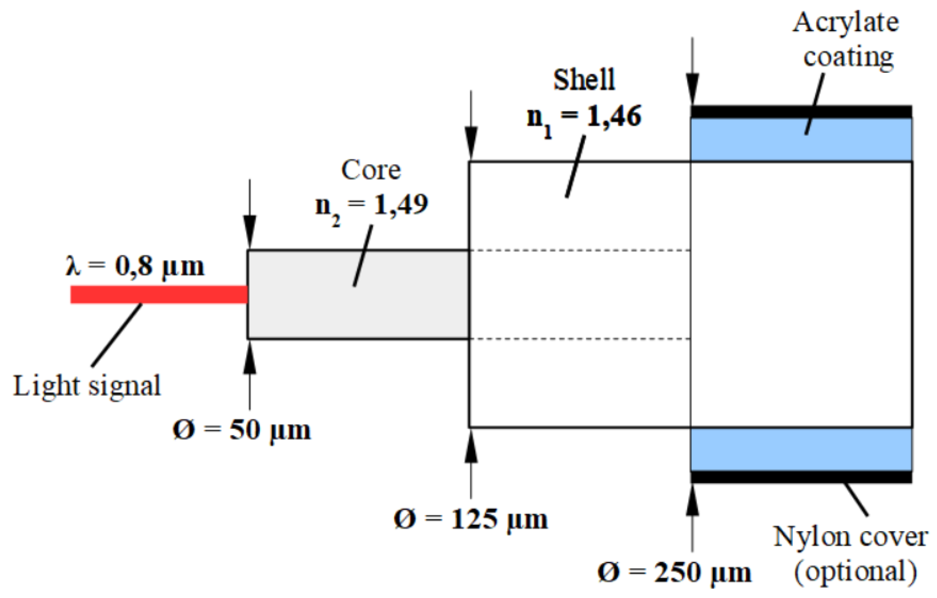
In Figure 1, the values of the shell and coating diameters, as well as the diameters of the inner layers, are average values accepted worldwide. However, depending on the type of fiber, the value of the core diameter and the refractive index can vary to a greater extent [22]. On the other hand, it is common that in daily use the fibers can be damaged and present problems in data transmission. Among the common problems, chromatic dispersion, absorption losses, scattering losses, bending losses, radiation losses, fiber connection losses, and connectors, among others, can be mentioned. The effects can be perceived by a decrease in bandwidth, attenuation, and decrease in the quality of the transmitted signal [22]. In this work, the losses caused by curvature will be studied, as they provide visual deformities that will be analyzed by the algorithms. These can be classified as macro curvatures and micro curvatures.

According to [22], macro bends are common when the cable is installed with a bend that has a radius smaller than the minimum bend radius. Light will hit the core/shell interface at an angle smaller than the critical angle, and therefore the optical beam will no longer remain confined within the core and will fade. An example of macro curvature can be seen in Figure 2.

Figure 2. Macro curvature example

Figure 2. Macro curvature example

As seen in Figure 2, a macro curvature can occur when the bend angle is smaller than the critical angle ${\theta }_c$, which produces transmission losses. On the other hand, micro-bends are minimal bends in the cable. This imperfection happens due to several reasons, but mainly due to external forces. As with macro curvatures, the light signal will hit the fold at an angle smaller than the critical angle and will be refracted to the shell [22], as seen in Figure 3.

Figure 3 shows how the arrows indicate the path taken by the light signal through the optical fiber. When there are micro-bends, as in this case, part of that light beam ends up fading.

Figure 3. Micro curvature example

Figure 3. Micro curvature example

3.2. VGG16 Neural Network

The VGG Neural Network was proposed by the Visual Geometry Group [23] intending to improve the network proposed by [24]; the difference regarding the network proposed by [24] was that the authors proposed to change the depth of the neural network architecture. The VGG network can have between 11 and 19 weight layers; the VGG-16 uses 16 layers, as can be seen in Figure 4.

Figure 4. Micro curvature example

Figure 4. Micro curvature example

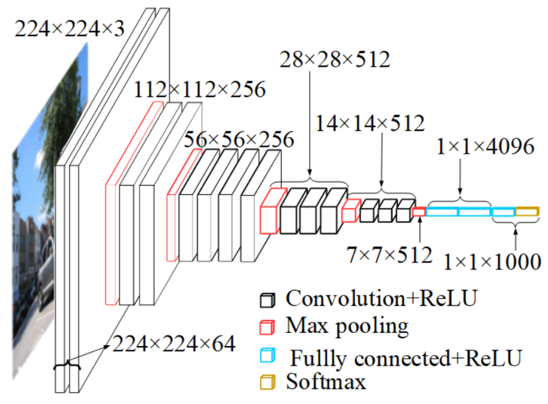
The input image for the first convolution layer is 224×224×3. The input image will go through a stack of convolutional layers that have filters with a small reception field of 3×3; that is the smallest size to detect the left/right, above/below, and center notions. The network has 3 fully connected layers and 5 max pooling layers. A ReLU rectifier is used for the hidden and fully connected layers, and a SoftMax is used for the last layer.

3.3. ResNet50 Neural Network

Residual nets, such as ResNet-50, are a series of deep convolutional neural networks first proposed by [25]. At first, as the number of layers rises, the accuracy also increases. But, after an inflection point, this stops being true because of the phenomenon of vanishing gradients.

Vanishing gradients are caused when training artificial neural networks with gradient-based learning methods and backpropagation, where the gradients, after each multiplication, can start achieving minimal values. This can cause the model to stagnate or even deteriorate the training for the model.

The residual network was also the first to introduce the concept of skip connections. This is a tool used for mitigating the problem of vanishing gradients. Instead of simply stacking convolutional layers one after another, the idea with ResNet was to skip some of these connections, which allows the network to be deeper than other architectures.

Figure 5 shows the architecture for a residual network with 50 layers. The skip connections, when they exist, are located inside the convolutional blocks.

Figure 5. Architecture of a ResNet-50 network

Figure 5. Architecture of a ResNet-50 network

4. Materials and Methods

4.1. Optical Fiber Dataset

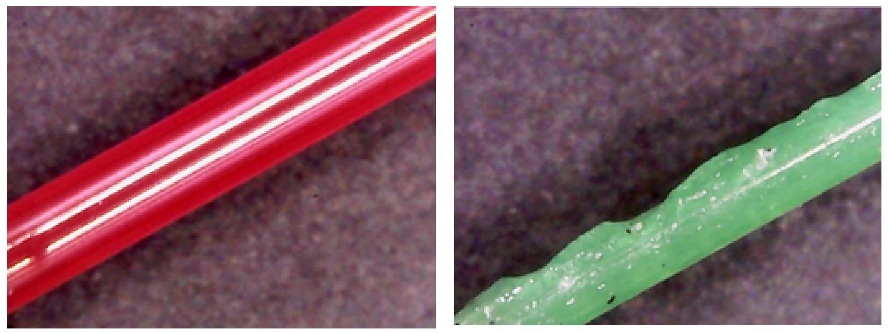
The initial dataset consists of 27 images of optical fiber cables in five different colors: red, blue, green, yellow, and white. This dataset is part of the work of previous research [2]. Figure 6 shows two cables that belong to the dataset that appear in different conservation and cleaning states. The right figure shows a new and clean red optical fiber cable. Optical fibers can suffer from several types of losses, such as macro- and micro-bending. In Figure 6 to the left, an example of optical fiber cable with micro-bending, purposely made, is shown.

Figure 6. Optical fibers: left figure in good condition and right figure with microbending and dirt.

Figure 6. Optical fibers: left figure in good condition and right figure with microbending and dirt.

4.2. Data Augmentation

Given that the number of images in the dataset is small, a very common technique for image classification was to use data augmentation. There are different methods of data augmentation, such as zooming, horizontal or vertical shifts, mirroring, rotations, and brightness tweaking. Two of these techniques were used: zooming and horizontal mirroring. Ranging through the intensities of these effects, a new dataset consisting of 440 images (along with the original 27) was conceived. Figure 7 shows the optical fiber dataset with data augmentation.

Figure 7. Optical fiber dataset with data augmentation

Figure 7. Optical fiber dataset with data augmentation

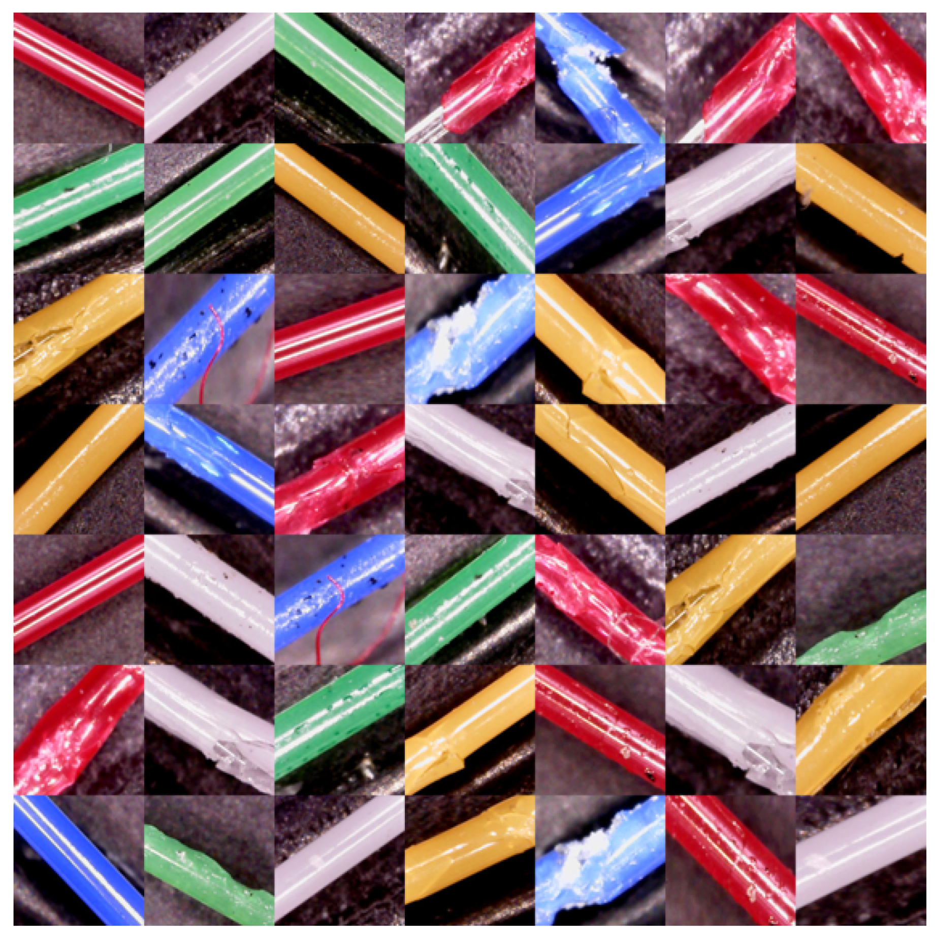
As shown in Figure 7, data-augmented images are very similar to their original counterparts. Although they have significant differences, such as variations in depth and the direction in which the fiber is exhibited.

4.3. Dataset Processing

Once the original dataset was artificially augmented and the number of images raised to 440, it was necessary to divide them into three subsets: training, validation, and test. The VGG-16 neural network was compiled with the parameters shown in Table 1.

Table 1. Parameters for the VGG-16 training

Parameter	Value
Metrics	Accuracy
Learning rate	$1e^{-4}$
Loss function	Categorical Cross Entropy

Table 1. Parameters for the VGG-16 training

Parameter	Value
Metrics	Accuracy
Learning rate	$1e^{-4}$
Loss function	Categorical Cross Entropy

The training lasted for 30 epochs. After training the VGG-16 neural network, the ResNet-50 algorithm was trained. Similarly, Table 2, below, refers to the parameters used for training the ResNet-50 network.

Table 2. Parameters for the ResNet-50 training

Parameter	Value
Optimizer	SGD (Stochastic Gradient Descent)
Learning rate	$1e^{-4}$
Loss function	Binary Cross Entropy

Table 2. Parameters for the ResNet-50 training

Parameter	Value
Optimizer	SGD (Stochastic Gradient Descent)
Learning rate	$1e^{-4}$
Loss function	Binary Cross Entropy

5. Results

The experiments using the methodology proposed in the paper will be presented in the following section.

5.1. VGG-16 Experiments

Both neural networks were modeled with the same epoch number. This is done to have a fair comparison; each epoch is a new try for the model to train and get better. Besides the epoch number, the same dataset was used in each training of the models.

Figure 8 shows the training accuracy in blue and the validation accuracy in orange obtained using the VGG-16 neural network based on 30 epochs.

Figure 8. Accuracies in training (blue) and validation (orange) of the VGG-16 algorithm

Figure 8. Accuracies in training (blue) and validation (orange) of the VGG-16 algorithm

The VGG-16’s training results were consistent with the model’s chosen setup. After 30 epochs, accuracy and loss function values start settling. Although the values vary considerably (as in Figure 9 Once the neural network models were trained and saved, it was possible to use them to predict. A confusion matrix with images from the test dataset was built. This confusion matrix is shown in Figure 9.

Figure 9. Confusion matrix of the VGG-16 neural network

Figure 9. Confusion matrix of the VGG-16 neural network

Based on the confusion matrix, it is possible to assume that the VGG-16 model’s difficulty was to correctly classify “bad” class fibers, because this was the class that showed more false positives.

5.2. ResNet-50 Experiments

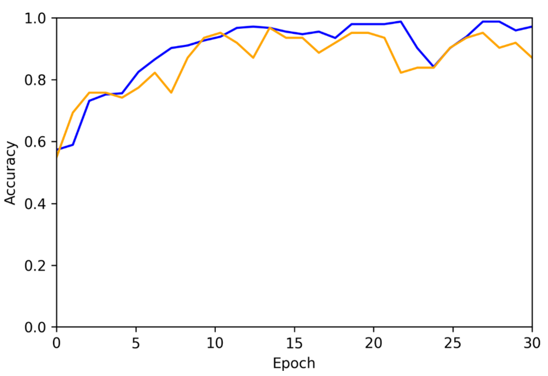
The ResNet-50 neural network was trained under the same conditions (30 epochs). Figure 10 shows the accuracy for the training in blue and the accuracy for the validation in orange for the ResNet-50 neural network. It was observed that the VGG-16 has a slower training compared to the ResNet-50. The ResNet-50 training starts to settle after 30 training epochs, discarding the need for a longer training.

Figure 10. Accuracy for the training (blue) and accuracy for the validation (orange) of the ResNet-50 algorithm

Figure 10. Accuracy for the training (blue) and accuracy for the validation (orange) of the ResNet-50 algorithm

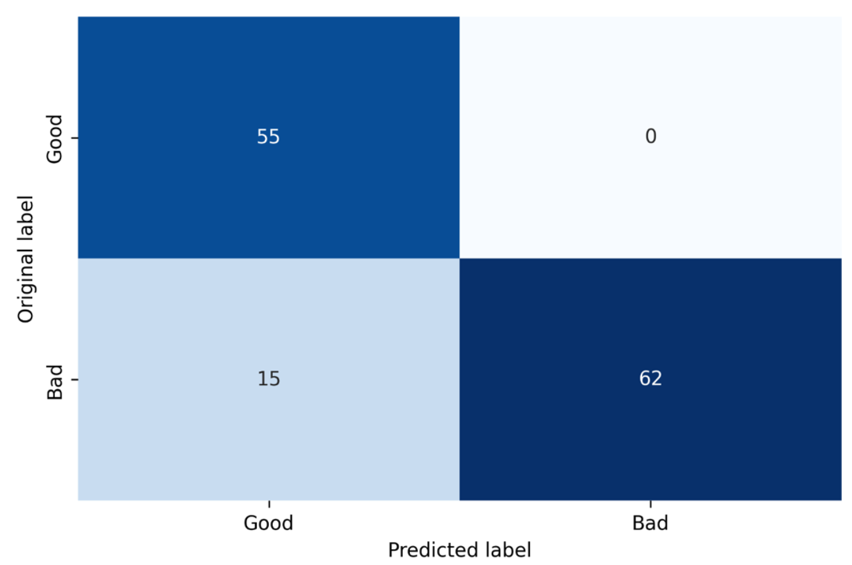
Superior results from the training dataset compared to validation in this case also help to affirm that the model did not suffer from overfitting. The confusion matrix of the ResNet-50 neural network is shown in Figure 11.

Figure 11. Confusion matrix of the ResNet-50 neural network

Figure 11. Confusion matrix of the ResNet-50 neural network

Table 3 shows a synthesis of the results obtained with the VGG-16 and ResNet-50 neural networks. In parallel to what is seen in classification by the VGG-16 algorithm, the biggest difficulty for the ResNet-50 model–—based on the confusion matrices—was in classifying correctly the “Good” class fibers. The number of false positives in this category was either higher or the same as the number of false positives in the other category. The data in the referred table synthesizes all the information from the confusion matrices.

Table 3. Confusion Matrix Results

Model	Class	Accuracy
VGG-16	Good	100%
VGG-16	Bad	80.52%
ResNet-50	Good	98.18%
ResNet-50	Bad	93.51%

Table 3. Confusion Matrix Results

Model	Class	Accuracy
VGG-16	Good	100%
VGG-16	Bad	80.52%
ResNet-50	Good	98.18%
ResNet-50	Bad	93.51%

Furthermore, if compared to the training time of both networks, the ResNet-50’s training time is inferior by almost half. Comparing the results obtained in this paper with our previous work, an accuracy of 86.95% was obtained for an optical fiber in good condition, and an accuracy of 88.57% was obtained for an optical fiber in bad condition. From the results shown in Table 3, it could be possible to infer that with the VGG-16 and ResNet-50 for a good condition, the results were better at 100% and 98.18%, and for a bad condition, the VGG-16 was not as good as the fuzzy system with 80.52%, but the ResNet was better with 93.51%, showing that, on average, the deep neural networks were better than the fuzzy system. Furthermore, in previous research, different image processing methods that enhance the complexity of the system — like the Hough transform, SURF and SIFT features, the Canny filter, and other image processing techniques — were used. With the employment of deep neural networks, the degree of complexity of the system is reduced, offering a simpler approach.

6. Conclusions

This work demonstrates that it is possible to use computational vision for optical fiber classification. Based on this premise, deep learning was successfully applied for optical fiber classification, and it used a dataset of optical fiber images captured with a camera. The data augmentation technique was also applied to generate more data for the algorithms training.

Two neural network architectures were tested, generating satisfactory results with both neural network architectures, the ResNet-50 and VGG-16. The ResNet-50 had better results compared to the VGG-16 for optical fiber images of the dataset. Although compared with our previous work using classic image processing techniques and fuzzy logic as a classifier, deep neural networks show more promising results, and their implementation was simpler. Finally, the optical fiber dataset was made available for anyone that would desire to test new algorithms of image processing for optical fibers. Future works could analyze the use of data fusion processes.

References

- Shahraray, B.; Schmidt, A.; Palmquist, J. Defect Detection, Classification and Quantification in Optical Fiber Connectors. 01 1990, pp. 15–22.
- Mafalda, M.; Welfer, D.; De Souza Leite Cuadros, M.A.; Gamarra, D.F.T. Image Processing Algorithm to Detect Defects in Optical Fibers. In Proceedings of the Fuzzy Information Processing; Barreto, G.A.; Coelho, R., Eds., Cham; 2018; pp. 243–252. [Google Scholar]
- Mafalda, M. Dataset Optical Fibers, 2022.
- Sinha, S.; Fieguth, P.W. . Morphological segmentation and classification of underground pipe images. Machine Vision and Applications 2006, 17. [Google Scholar] [CrossRef]
- Hagele, C.; Frizero Neto, A.P.M. Polymer Optical Fiber Curvature Measuring Technique Based on Speckle Pattern Image Processing. In In Proceedings of the In Simpósio Brasileiro de Automação Inteligente; 2015. [Google Scholar]
- Xiao-rong, C. , Yuan C., C.l.X. Research on the Algorithm about Optical Fiber Parameters Measurement. TELKOMNIKA 2013, 11, 6693–6698. [Google Scholar] [CrossRef]
- Leal Junior, A.; Frizera, A.; Marques, C.; Alfonso Sánchez, M.; Miranda dos Santos, W.; Siqueira, A.; Segatto, M.; Pontes, M. Polymer Optical Fiber for Angle and Torque Measurements of a Series Elastic Actuator’s Spring. Journal of Lightwave Technology 2018, 1–1. [Google Scholar] [CrossRef]
- Domingues, F.; Tavares, C.; Leitão, C.; Frizera, A.; Alberto, N.; Marques, C.; Radwan, A.; Rodriguez, J.; Postolache, O.; Rocon, E.; et al. Insole optical fiber Bragg grating sensors network for dynamic vertical force monitoring. Journal of Biomedical Optics 2017, 22, 091507–091507. [Google Scholar] [CrossRef] [PubMed]
- Leal Junior, A.; Frizera, A.; Marques, C.; Alfonso Sánchez, M.; Botelho, T.; Segatto, M.; Pontes, M. Polymer optical fiber strain gauge for human-robot interaction forces assessment on an active knee orthosis. Optical Fiber Technology 2018, 41, 205–211. [Google Scholar] [CrossRef]
- Leal Junior, A.; Frizera, A.; Marques, C.; Pontes, M. A Polymer Optical Fiber Temperature Sensor Based on Material Features. Sensors (Basel, Switzerland) 2018, 18, 1–1. [Google Scholar] [CrossRef] [PubMed]
- Diaz, C.; Leal Junior, A.; André, P.; Antunes, P.; Pontes, M.; Frizera, A.; Ribeiro, M. Liquid Level Measurement Based on FBG-Embedded Diaphragms With Temperature Compensation. IEEE Sensors Journal 2017, 1–1. [Google Scholar] [CrossRef]
- Leal Junior, A.; Diaz, C.; Avellar, L.; Pontes, M.; Marques, C.; Frizera, A. Polymer Optical Fiber Sensors in Healthcare Applications: A Comprehensive Review. Sensors 2019, 19, 3156. [Google Scholar] [CrossRef] [PubMed]
- Ajmi, C.; Zapata Pérez, J.; Ferchichi, S.; Zaafouri, A.; Laabidi, K. Deep Learning Technology for Weld Defects Classification Based on Transfer Learning and Activation Features. Advances in Materials Science and Engineering 2020, 2020, 16. [Google Scholar] [CrossRef]
- Victor Ikechukwu, A.; Murali, S.; Deepu, R.; Shivamurthy, R. ResNet-50 vs VGG-19 vs training from scratch: A comparative analysis of the segmentation and classification of Pneumonia from chest X-ray images. Global Transitions Proceedings 2021, 2, 375–381, International Conference on Computing System and its Applications (ICCSA- 2021). [Google Scholar] [CrossRef]
- Shin, H.c.; Roth, H.; Gao, M.; Lu, L.; Xu, Z.; Nogues, I.; Yao, J.; Mollura, D.; Summers, R. Deep Convolutional Neural Networks for Computer-Aided Detection: CNN Architectures, Dataset Characteristics and Transfer Learning. IEEE Transactions on Medical Imaging 2016, 35. [Google Scholar] [CrossRef] [PubMed]
- Lv, Y.; Zhou, W.; Tian, Q.; Sun, S.; Li, H. Retrieval Oriented Deep Feature Learning With Complementary Supervision Mining. IEEE Transactions on Image Processing 2018, 1–1. [Google Scholar] [CrossRef] [PubMed]
- Yun, J.; Chen, L.; Zhang, H.; Xiao, X. Breast cancer histopathological image classification using convolutional neural networks with small SE-ResNet module. PLoS ONE 2019, 14. [Google Scholar] [CrossRef]
- Kaur, T.; Gandhi, T. Automated Brain Image Classification Based on VGG-16 and Transfer Learning. 12 2019, pp. 94–98. [CrossRef]
- Ramzan, F.; Khan, M.U.; Rehmat, A.; Iqbal, S.; Saba, T.; Rehman, A.; Mehmood, Z. A Deep Learning Approach for Automated Diagnosis and Multi-Class Classification of Alzheimer’s Disease Stages Using Resting-State fMRI and Residual Neural Networks. Journal of Medical Systems 2019, 44. [Google Scholar] [CrossRef] [PubMed]
- Mikołajczyk, A.; Grochowski, M. Data augmentation for improving deep learning in image classification problem. 05 2018, pp. 117–122. [CrossRef]
- Keiser, G. Optical Fiber Communications; McGraw-Hill Education (India) Private Limited, 2013.
- Bailey, D.; Wright, E. Practical Fiber Optics; Elsevier Science, 2003.
- Simonyan, K.; Zisserman, A. Very Deep Convolutional Networks for Large-Scale Image Recognition. arXiv, 2014; arXiv:1409.1556. [Google Scholar]
- Krizhevsky, A.; Sutskever, I.; Hinton, G. ImageNet Classification with Deep Convolutional Neural Networks. Neural Information Processing Systems 2012, 25. [Google Scholar] [CrossRef]
- He, K.; Zhang, X.; Ren, S.; Sun, J. Deep Residual Learning for Image Recognition. In Proceedings of the 2016 IEEE Conference on Computer Vision and Pattern Recognition (CVPR); 2016; pp. 770–778. [Google Scholar] [CrossRef]
Disclaimer/Publisher’s Note: The statements, opinions and data contained in all publications are solely those of the individual author(s) and contributor(s) and not of MDPI and/or the editor(s). MDPI and/or the editor(s) disclaim responsibility for any injury to people or property resulting from any ideas, methods, instructions or products referred to in the content. |
© 2025 by the authors. Licensee MDPI, Basel, Switzerland. This article is an open access article distributed under the terms and conditions of the Creative Commons Attribution (CC BY) license (https://creativecommons.org/licenses/by/4.0/).
Copyright: This open access article is published under a Creative Commons CC BY 4.0 license, which permit the free download, distribution, and reuse, provided that the author and preprint are cited in any reuse.