
Submitted:
02 November 2025
Posted:
04 November 2025
You are already at the latest version
Abstract
Reconstructing medical images from partial measurements is a critical inverse problem in Computer Tomography, essential for reducing radiation exposure while maintaining diagnostic accuracy, addressing challenges of small size and poor resolution in CT data. Existing solutions based on machine learning typically train a model to directly map measurements to medical images, relying on a training dataset of paired images and measurements synthesized using a fixed physical model of the measurement process; however, this approach greatly hinders generalization to unknown measurement processes. To address this issue, we propose a fully unsupervised technique for solving the inverse problem, leveraging score-based generative models to eliminate the need for paired data. Specifically, we first train a score-based generative model on clean conventional-dose medical images to capture their prior distribution. Then, given measurements and a physical model of the measurement process, we introduce a sampling method to reconstruct an image consistent with both the prior and the measurements. Empirically, we observe comparable or better performance to other sampling techniques in several medical imaging tasks in Computer Tomography, while demonstrating considerably better generalization to unknown measurement processes. The code is available.
Keywords:
score-based generative model
; controllable generation
; projection to convex set
; filter back projection
; iterative reconstruction
1. Introduction
With the advancement of machine learning, numerous methods have been proposed for reconstructing medical images from limited measurements [1,2,3,4,5,6]. Most of these approaches rely on supervised learning, where models are trained to directly map partial measurement data to reconstructed images using large datasets consisting of paired CT images and corresponding measurements. These measurements are typically generated by simulating a fixed physical model of the imaging process. However, when the measurement process changes — for example, when the number of CT projections is altered — it becomes necessary to regenerate the training dataset using the new acquisition settings and retrain the model from scratch. This process is both time-consuming and resource-intensive. Moreover, it limits the model’s ability to generalize across different acquisition conditions, and in some cases, may even lead to counterintuitive results, such as degraded performance with more measurements [7]. In this work, we address the aforementioned challenge by introducing unsupervised methods that eliminate the need for paired datasets during training, thus removing the dependency on a fixed measurement process. Our core idea is to model the prior distribution of medical images using a generative approach, which allows us to recover missing information resulting from incomplete measurements. Concretely, we train a score-based generative model[8,9] on a collection of high-quality medical images to serve as a data prior. Once trained, we employ a classifier-free [10] controllable sampling algorithm that generates images consistent with both the observed measurements and the learned prior, while incorporating the physical characteristics of the measurement process. Importantly, after training, the model can be flexibly applied to solve inverse problems within the same image domain, provided the measurement operator remains linear.
We evaluate the proposed method across multiple CT reconstruction tasks. Empirically, our approach achieves performance that is on par with or superior to existing unsupervised learning methods [11,12], even when all methods are trained and tested under the same measurement settings. Furthermore, when the measurement conditions are altered—for instance, by varying the number of projections in sparse-view CT—our method consistently outperforms all competing approaches. These empirical results collectively demonstrate that our method not only serves as a strong alternative to current unsupervised techniques in medical image reconstruction and artifact suppression but also shows great potential as a general-purpose framework for solving a wide range of inverse problems within the same image domain.
2. Background
2.1. Variational Diffusion Models
For many modalities, we can think of the data we observe as represented or generated by an associated unseen latent variable. The best intuition for expressing this idea is through Plato’s Allegory of the Cave. In this allegory, a group of people are chained inside a cave their entire life and can only see the two-dimensional shadows projected onto a wall in front of them, which are generated by unseen three-dimensional objects passed before a fire, as Figure 1 shows.
In generative modeling, observed data can be interpreted as a low-dimensional projection or manifestation of latent variables residing in a more complex, hidden space. These latent variables encapsulate high-level abstract features such as color, size, shape, and other semantic attributes. The objects we perceive in the real world can therefore be understood as realizations or projections of these latent concepts into observable form, analogous to how the cave dwellers perceive only shadows of unseen objects. While the individuals in the cave cannot observe the true sources directly, they may still reason about their existence. Likewise, in generative modeling, we aim to approximate these latent representations to understand and reconstruct the observed data.
2.1.1. Variational Autoencoders
In the default formulation of the Variational Autoencoder (VAE)[13,14], we directly maximize the ELBO. This approach is variational, because we optimize for the best amongst a family of potential posterior distributions parameterized by . It is called an autoencoder because it is reminiscent of a traditional autoencoder model, where input data is trained to predict itself after undergoing an intermediate bottlenecking representation step. To make this connection explicit, we rewrite the ELBO term:
The first term is the reconstruction term, and the second term is the prior matching term. In this case, we learn an intermediate bottlenecking distribution that can be treated as an encoder; it transforms inputs into a distribution over possible latents. Simultaneously, we learn a deterministic function to convert a given latent code z into an observation x, which can be interpreted as a decoder.
The KL divergence term (prior matching term) could be computed analytically, and the reconstruction term can be approximated using a Monte Carlo estimate. With this, we rewrite the objective function as:
where latents are sampled from , for every observation x in the dataset. After that, we use the reparameterization trick to conquer the non-differentiable problem, eventually getting:
In a VAE, each z is thus computed as a deterministic function of input x and auxiliary noise variable . Under this reparameterized version of z, gradients can then be computed for as desired. See Figure 2.
2.1.2. Hierarchical Variational Autoencoders
A Hierarchical Variational Autoencoder (HVAE)[15,16] (See Figure 3) is a generalization of a VAE that extends to multiple hierarchies over latent variables. Under this formulation, latent variables themselves are interpreted as generated from other higher-level, more abstract latents. Whereas in the general HVAE with T hierarchical levels, each latent is conditioned on all previous latents, in this work, we focus on a special case, which we call a Markovian HVAE (MHVAE). In a MHVAE, the generative process is a Markov chain, i.e., each transition down the hierarchy is Markovian, where decoding each latent only conditions on the previous latent . Mathematically, we represent the joint distribution and the posterior of a Markovian HVAE as:
Substituting the original ELBO expression, we get the new objective:
2.1.3. Unconditional Score-based Generative Model
The Variational diffusion model[17,18,19] formulation has an equivalent Score-based Generative Modeling formulation. Arbitrary probability distributions can be written in the form:
where is the energy function, often modeled by a neural network, and is a normalizing constant to ensure that . One way to avoid modeling the normalization constant is to use a neural network to learn the score function of distribution instead. This comes from taking the derivative of the ln of both sides of the equation above:
The equation above could be represented as a neural network without involving any normalization constants. The score model could be optimized by minimizing the Fisher Divergence with the ground truth score function:
The score function defines a vector field over the entire space where the data x lies, pointing towards the modes. Then, by learning the score function of the true data distribution, we can generate samples by starting at an arbitrary point in the same space and iteratively following the score until a mode is reached. This sampling procedure is known as Langevin dynamics, and is mathematically described as:
The initial value is randomly sampled from a prior distribution. Eventually, we can choose a positive sequence of noise scale and then define a sequence of progressively perturbed data distributions:
Then, a neural network is learned using denoising score matching to learn the score function for all noise levels:
where is a positive weighting function that conditions on noise level t. Furthermore, Song[9] proposes annealed Langevin Dynamics sampling as a generative procedure. The initialization is chosen from some hand-made prior, and each subsequent sampling step starts from the final samples of the previous simulation. This is analogous to the sampling procedure performed in the Markovian HVAE interpretation of a Variational Diffusion Model, where a randomly initialized data vector is iteratively refined over decreasing noise levels. Under an infinite number of noise scales, the perturbation of an image over continuous time can be represented as a stochastic process, and therefore described by a stochastic differential equation (SDE). Sampling is then performed by reversing the SDE, which naturally requires estimating the score function at each continuous-valued noise level. Different parameterizations of the SDE essentially describe different perturbation schemes over time. In this work, we use Variance Exploring (VE) SDE (See Figure 4 as a reference).
2.1.4. Classifier-Free Guidance
Because learning two separate diffusion models is expensive, in this work, we just consider the classifier-free guidance[10,20,21]. To derive the score function under Classifier-Free Guidance, first, we have:
Then, substituting this into the classifier-guidance equation , get:
The first term on the right-hand is the conditional score, and the second term is the unconditional score. is a term that controls how much the learned conditional model cares about the conditioning information. When , the learned conditional model completely ignores the conditioner and makes an unconditional inference; when , the model explicitly learns the vanilla conditional distribution without guidance; when , the diffusion model not only prioritizes the conditional score function, but also moves in the direction away from the unconditional score function.
2.2. Sparse-View Computer Tomography Inverse Problems
An inverse problem aims to recover an unknown signal from a set of observed measurements. Formally, let denote the unknown signal, and let represent the observed measurements modeled by the linear relation , where is the measurement operator and is the additive noise. The task of solving the inverse problem involves estimating from the noisy observation . When , the system is underdetermined, making the problem ill-posed unless additional prior knowledge about is introduced. To address this, we assume that follows a prior distribution . In the probabilistic formulation, the relationship between measurements and the signal is captured by the likelihood function , where denotes the noise distribution. Given both the likelihood and the prior , the inverse problem can be solved by inferring the posterior distribution and sampling from it.
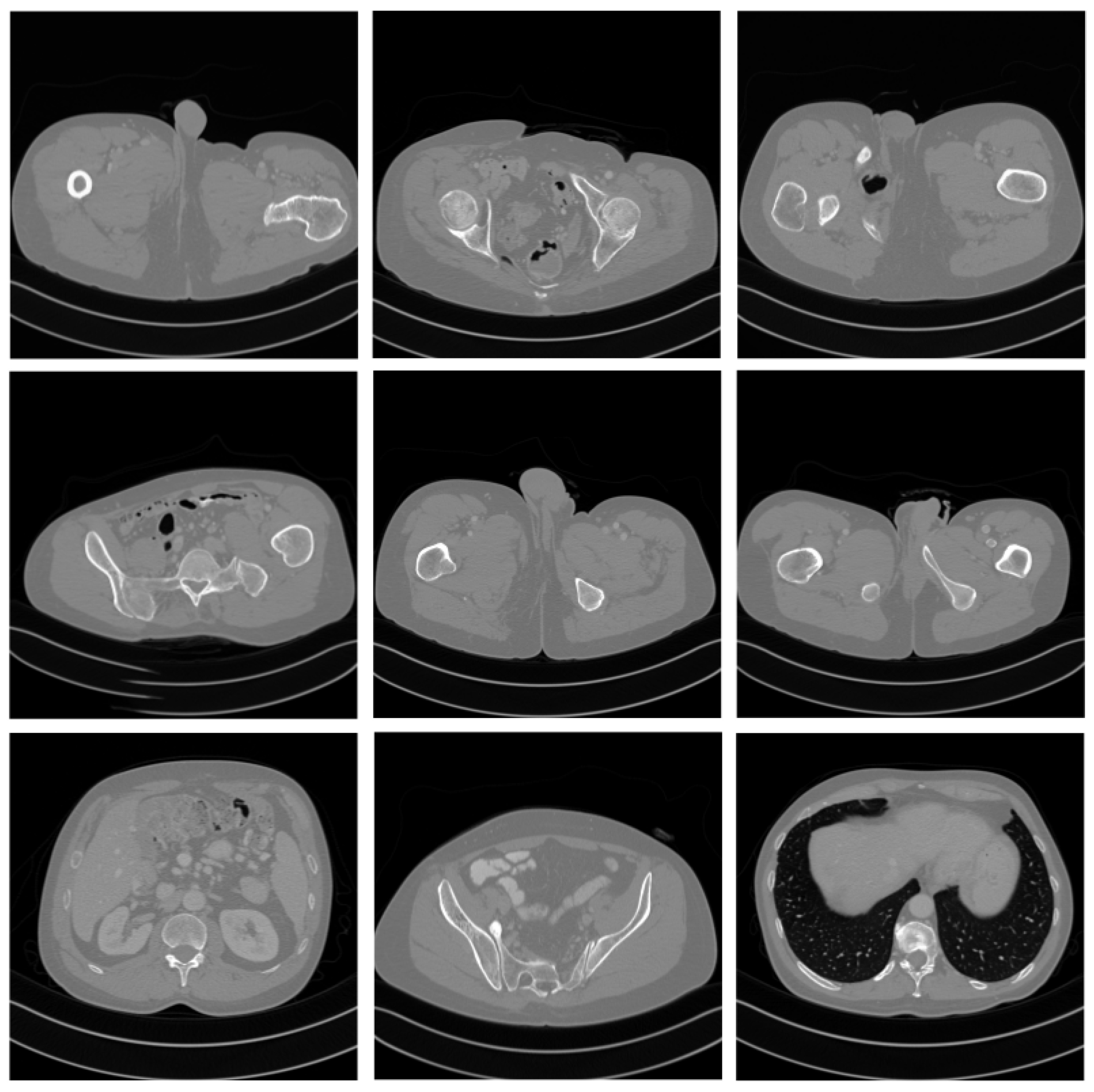
Figure 5.
Some unconditional samples. They look very realistic, but in fact, they have no reasonable anatomical structure. This is precisely the reason why guiding signals are needed.
Figure 5.
Some unconditional samples. They look very realistic, but in fact, they have no reasonable anatomical structure. This is precisely the reason why guiding signals are needed.
3. Methodology
3.1. Projection Onto Convex Sets (POCS)
In mathematics, projection onto convex sets (POCS), sometimes known as the alternating projection method, is a method to find a point in the intersection of two closed convex sets. The case when the sets are affine spaces is special, since the iterates not only converge to a point in the intersection, assuming the intersection is non-empty, but to the orthogonal projection of the point onto the intersection. POCS always has the following iteration form:
where denotes projecting data x onto the data fidelity set, and denotes projecting data x onto the prior set.
3.2. Imputation in the Radon Domain
Imputation is a special case of conditional sampling. The known and unknown dimensions of are denoted by and respectively, and let and denote the drift coefficient and the diffusion coefficient restricted to the unknown dimensions respectively. For VE SDEs, the drift coefficient is element-wise, and the diffusion coefficient is diagonal. So, when is element-wise, denotes the same element-wise function applied only to the unknown dimensions; when is diagonal, denotes the sub-matrix restricted to unknown dimensions.
In this setting, specifically denotes the samples transformed by the forward model from the diffusion model at each timestep, and denotes the constraint coming from the forward model. Because the Radon transform operator is not orthogonal, we need an orthogonal term analogous to the filtering step to implement the orthogonal projection, to make POCS work well.
3.3. PC-POCS Sampling
Combining POCS with the PC sampling method, we derive the PC-POCS algorithm. Specifically, we use the discretized timestep, from to , each timestep conducts two steps of update. The first step is used to predict the diffusion trajectory:
which always has the form of
The second step is used to correct the trajectory. The first part of the second step is Langevin correct:
After the corrector, come into the Kaczmarz iteration to satisfy the projection consistency:
where denotes the forward radon projection operator, denotes the back projection operator, denotes the filter back projection operator. denotes the measurement, i.e., sparse-view sinogram, and denotes the stepsize scheduler coefficient, denotes the normalization constant. The details of the whole algorithm are in the pseudocode.
| Algorithm 1 PC-POCS |
|
4. Experiment
For all tasks, we aim to verify the superiority of our method against other diffusion model-based approaches.
4.1. Dataset
We take the dataset from the AAPM 2016 CT low-dose grand challenge, where the data are acquired in a fan-beam geometry with varying parameters. The data preparation steps follow those of [22]. From the helical cone beam projections, an approximation to fanbeam geometry is performed via a single-slice rebinning technique. Reconstruction is then performed via standard filtered backprojection (FBP), where the reconstructed axial images have a matrix size of . We resize the axial slices to have the size , and use these slices to train the score function. The whole dataset consists of 9 volumes (3142 slices) of training data, and 1 volume (823 slices) of testing data. To generate sparse-view measurements, we retrospectively employ the parallel-view geometry for simplicity.
4.2. Details of Network Training
For the CT score function, we train the ncsnpp network with setting , and . Training is conducted by using two RTX 3080 Ti for 100 epochs, and the average loss eventually converges to .
4.3. Evaluation Metrics
We use three standard metrics: SSIM, PSNR, and FSIM for quantitative evaluation. FSIM may be a relatively novel metric, and makes an improvement on the SSIM, introducing phase consistency with position as a variable and weighting the SSIM based on this. The basic formula of FSIM is:
The equation above expresses the image signal as a Fourier series expansion, where each component has a corresponding phase. represents the average phase of all components, denotes the phase of each individual component, and is the amplitude.
4.4. Comparative Experiment with the State-of-the-Art Methods
To the best of our knowledge, [11,12] are the only two methods that solve CT reconstruction directly with diffusion models. So, we compare our method against theirs. We call the method from [11] as Song, and the approach from [12] as MCG. To control the variables, the experiments of the three methods were all conducted under the condition of sparsity of 6 (i.e., the number of projections was 30). The numerical results of the experiment are shown in Table 1, and the visualization results are shown in Figure 6.
From Table 1, we could see that the PC-POCS method outperforms the other two methods in terms of all three metrics, whether the max value or the second best value among all the slices of patient L096 shown. In addition, we also presented some reconstruction results to provide a more intuitive feeling. See supplement material. Visually, under the sparsity of 6 (30 projections), the PC-POCS method has the best visual effect.
4.5. Ablation Study
For different methods, determining the lower bound of sparsity is a very important task. Generally speaking, the higher the sparsity, the worse the quality of the reconstructed image. For instance, taking SSIM as the standard, the SSIM of reliably reconstructed images in medicine is generally greater than . Reconstructed images below this lower bound, due to the loss of most of the true structure, will not have clinical value.
Due to this consideration, we conducted an ablation experiment to determine the sparsity corresponding to the minimum trusted image. The relationship between the sparsity and the number of projections is:
From Figure 8, the relationship between the sparsity (number of projections) and metrics is obvious. For the integrity of the experiment, we also conducted experiments on FSIM and PSNR, and provided the results. According to Figure 8, when , the SSIM reaches the lower bound of 0.7.
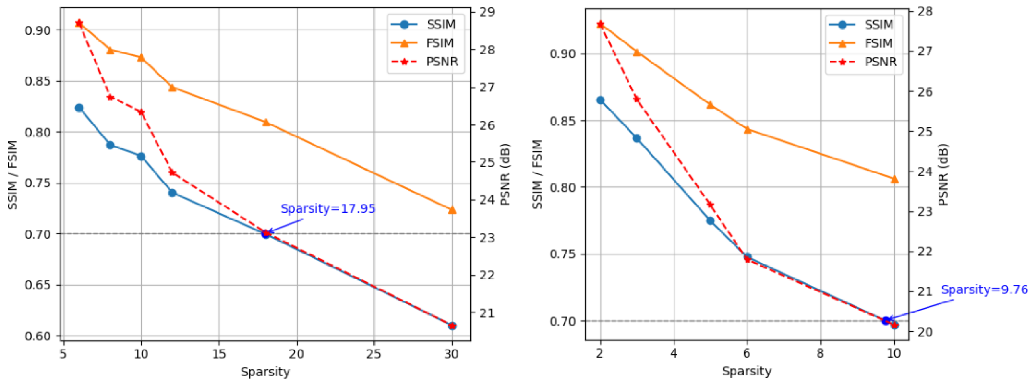
For the sake of demonstrating the performance of our method, we conduct an ablation study on the other two methods. The experiment result is shown in Figure 9. Besides that, the visualization results of this ablation study are also provided in Figure 7. Our proposed method needs less physical information than the other two methods and has the highest threshold sparsity for reconstruction.
Figure 7.
The ablation study result of slice 290 of patient L096. From left to right, the images correspond to different sparsity levels. From upwards to downwards, the images correspond to ground truth, PC-POCS, MCG, and Song, respectively. For PC-POCS, the sparsity is set to . Because the quality of the image is very low under the method of Song, we just set the sparsity of for reference. We find that under high sparsity, some subtle structure is lost, for example, the part in the white border is different in the ground truth and the reconstruction under high sparsity. You can zoom in to see more details of the image.
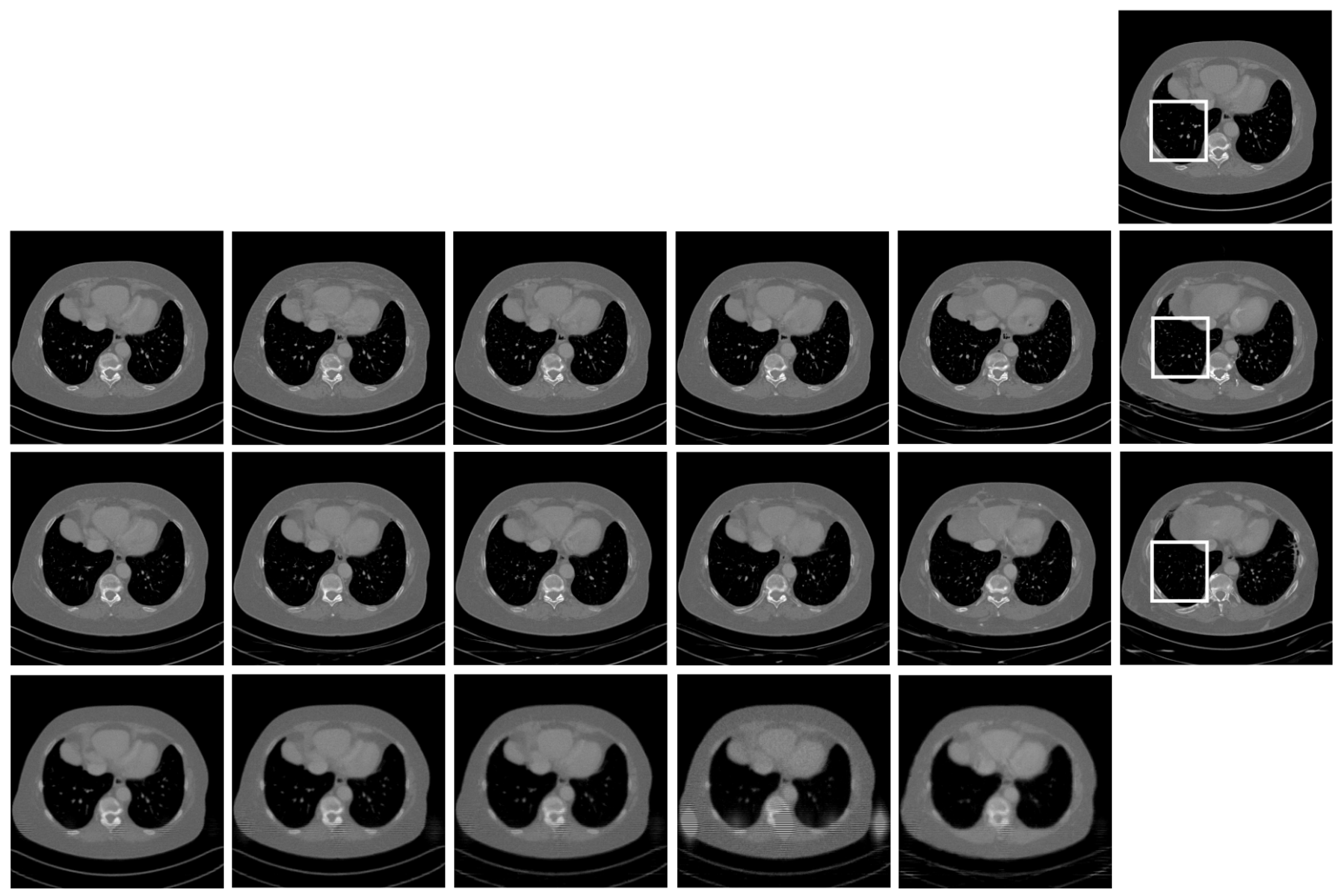
Figure 8.
The relationship between the sparsity and each metric. With the increase of sparsity, the number of projections decreases, so the true physical information decreases, and the quality of the reconstruction images deteriorates. According to the plot, when sparsity = 26, the SSIM reaches the threshold of 0.7.
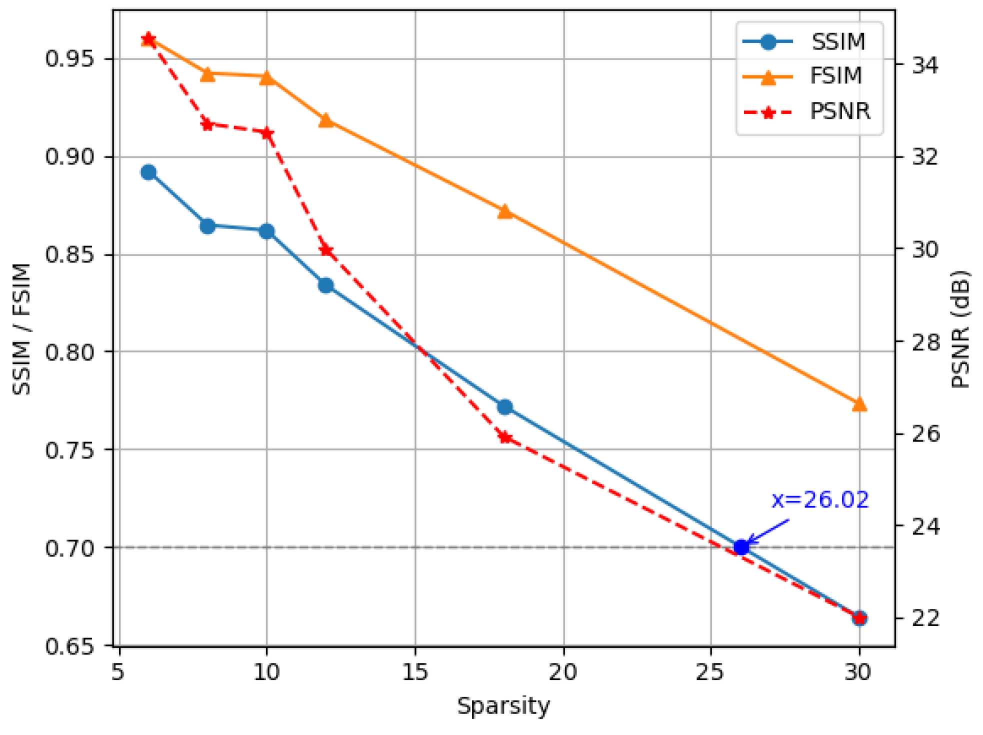
Figure 9.
MCG(left) and Song(right)’s ablation study results. The threshold sparsity is 18, 10, respectively. The bigger the numerical value is, the more physical information the method needs. So from this perspective, our proposed method also outperforms the other two methods.
Figure 9.
MCG(left) and Song(right)’s ablation study results. The threshold sparsity is 18, 10, respectively. The bigger the numerical value is, the more physical information the method needs. So from this perspective, our proposed method also outperforms the other two methods.
5. Conclusion
In this work, we proposed a general framework that can greatly enhance the performance of the score-based generative model’s solver for solving the low-dose computer tomography inverse problem. We show that our method can outperform the current state-of-the-art method. In addition, we conduct an ablation study on the proposed method, the result shows that our method could work under high sparsity with a reliable reconstruction result, and also has a stronger ability than the other two methods.
5.1. Limitations
The proposed method is intrinsically stochastic, as it fundamentally relies on the diffusion model. When the measurement dimension m is significantly reduced, the method occasionally fails to yield high-quality reconstructions, although it still generally outperforms competing approaches.
Furthermore, we acknowledge that our method is relatively slow in generating samples, as it inherits the limitations of diffusion models. This limitation could potentially be mitigated by incorporating recent solvers designed to accelerate diffusion model inference.
5.2. Broader Impact
Aligned with the concerns associated with generative model-based approaches to inverse problems, our method’s strong reliance on the underlying diffusion model raises the potential for generating harmful content, such as deepfakes. In addition, it may amplify pre-existing social biases embedded in the training dataset.
Data Availability Statement
The data used in this study are publicly available from the AAPM Low-Dose CT Grand Challenge dataset (https://www.aapm.org/GrandChallenge/LowDoseCT/).
Conflicts of Interest
The authors declare that they have no conflict of interest.
References
- Zhu, B., Liu, J., Cauley, S. et al. Image reconstruction by domain-transform manifold learning. Nature 555, 487–492 (2018). [CrossRef]
- Morteza Mardani, Enhao Gong, Joseph Y Cheng, Shreyas Vasanawala, Greg Zaharchuk, Marcus Alley, Neil Thakur, Song Han, William Dally, John M Pauly, et al. Deep generative adversarial networks for compressed sensing automate MRI. arXiv preprint, 2017. arXiv:1706.00051.
- Liyue Shen, Wei Zhao, and Lei Xing. Patient-specific reconstruction of volumetric computed tomography images from a single projection view via deep learning. Nature biomedical engineering, 3(11):880–888, 2019. [CrossRef]
- Tobias Würfl, Mathis Hoffmann, Vincent Christlein, Katharina Breininger, Yixin Huang, Mathias Unberath, and Andreas K Maier. Deep learning computed tomography: Learning projection domain weights from image domain in limited angle problems. IEEE transactions on medical imaging, 37(6):1454–1463, 2018. [CrossRef]
- Muhammad Usman Ghani and W Clem Karl. Deep learning-based sinogram completion for low-dose CT. In 2018 IEEE 13th Image, Video, and Multidimensional Signal Processing Workshop (IVMSP), pp. 1–5. IEEE, 2018.
- Haoyu Wei, Florian Schiffers, Tobias Würfl, Daming Shen, Daniel Kim, Aggelos K Katsaggelos, and Oliver Cossairt. 2-step sparse-view CT reconstruction with a domain-specific perceptual network. arXiv preprint, 2020. arXiv:2012.04743.
- Vegard Antun, Francesco Renna, Clarice Poon, Ben Adcock, and Anders C Hansen. On instabilities of deep learning in image reconstruction and the potential costs of AI. Proceedings of the National Academy of Sciences, 117(48):30088–30095, 2020. [CrossRef]
- Yang Song and Stefano Ermon. Generative modeling by estimating gradients of the data distribution. In Advances in Neural Information Processing Systems, pp. 11918–11930, 2019.
- Yang Song, Jascha Sohl-Dickstein, Diederik P Kingma, Abhishek Kumar, Stefano Ermon, and Ben Poole. Score-based generative modeling through stochastic differential equations. In International Conference on Learning Representations, 2021. URL https://openreview.net/forum? id=PxTIG12RRHS.
- Sander Dieleman. Guidance: a cheat code for diffusion models, 2022. URL https://benanne.github.io/2022/ 05/26/guidance.html.
- Yang Song, Liyue Shen, Lei Xing, and Stefano Ermon. Solving inverse problems in medical imaging with score-based generative models. In International Conference on Learning Representations, 2022.
- Hyungjin Chung, Byeongsu Sim, Dohoon Ryu, and Jong Chul Ye. 2022. Improving diffusion models for inverse problems using manifold constraints. In Proceedings of the 36th International Conference on Neural Information Processing Systems (NIPS ’22). Curran Associates Inc., Red Hook, NY, USA, Article 1862, 25683–25696.
- Diederik P Kingma and Max Welling. Auto-encoding variational bayes. arXiv preprint, 2013. arXiv:1312.6114.
- Danilo Jimenez Rezende, Shakir Mohamed, and Daan Wierstra. Stochastic backpropagation and approximate inference in deep generative models. In International Conference on machine learning, pages 1278–1286. PMLR, 2014.
- Durk P Kingma, Tim Salimans, Rafal Jozefowicz, Xi Chen, Ilya Sutskever, and Max Welling. Improved variational inference with inverse autoregressive flow. Advances in neural information processing systems, 29, 2016.
- Casper Kaae Sønderby, Tapani Raiko, Lars Maaløe, Søren Kaae Sønderby, and Ole Winther. Ladder variational autoencoders. Advances in neural information processing systems, 29, 2016.
- Jascha Sohl-Dickstein, Eric Weiss, Niru Maheswaranathan, and Surya Ganguli. Deep unsupervised learning using nonequilibrium thermodynamics. In International Conference on Machine Learning, pages 2256–2265. PMLR, 2015.
- Jonathan Ho, Ajay Jain, and Pieter Abbeel. Denoising diffusion probabilistic models. Advances in Neural Information Processing Systems, 33:6840–6851, 2020.
- Diederik Kingma, Tim Salimans, Ben Poole, and Jonathan Ho. Variational diffusion models. Advances in neural information processing systems, 34:21696–21707, 2021.
- Chitwan Saharia, William Chan, Saurabh Saxena, Lala Li, Jay Whang, Emily Denton, Seyed Kamyar Seyed Ghasemipour, Burcu Karagol Ayan, Sara Mahdavi, Rapha Gontijo Lopes, et al. Photorealistic text-to-image diffusion models with deep language understanding. arXiv preprint, 2022. arXiv:2205.11487.
- Jonathan Ho and Tim Salimans. Classifier-free diffusion guidance. In NeurIPS 2021 Workshop on Deep Generative Models and Downstream Applications, 2021.
- Eunhee Kang, Junhong Min, and Jong Chul Ye. A deep convolutional neural network using directional wavelets for low-dose X-ray CT reconstruction. Medical physics, 44(10):e360–e375, 2017. [CrossRef]
Figure 1.
Plato’s Cave, drawn by Sanraedam. People in the Cave could never see the real latent world because of the dimension they live in.
Figure 1.
Plato’s Cave, drawn by Sanraedam. People in the Cave could never see the real latent world because of the dimension they live in.
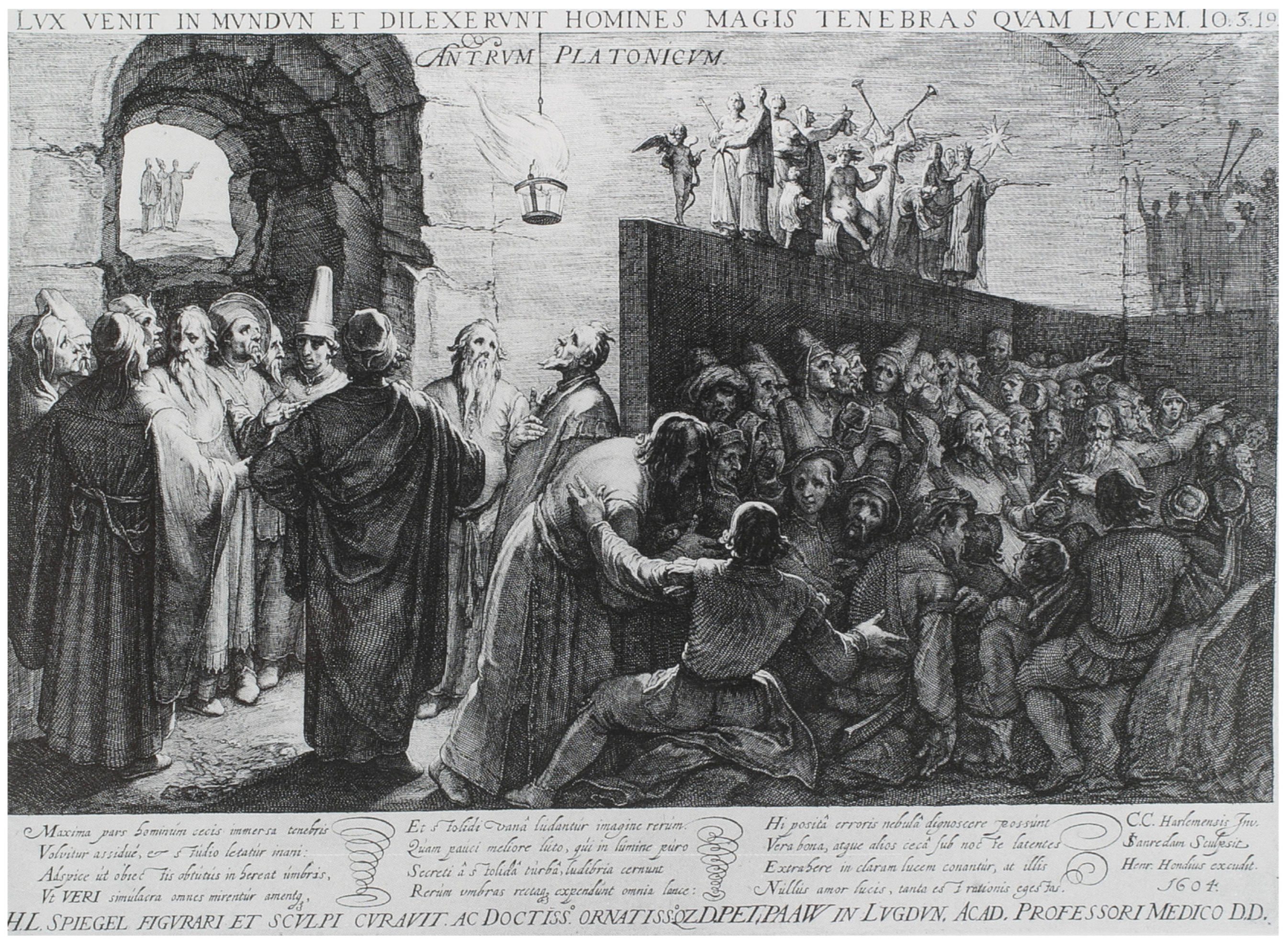
Figure 2.
A Variational Autoencoder graphically represented. Encoder defines a distribution over latent variables z for observations x, and decodes latent variables into observations.
Figure 2.
A Variational Autoencoder graphically represented. Encoder defines a distribution over latent variables z for observations x, and decodes latent variables into observations.
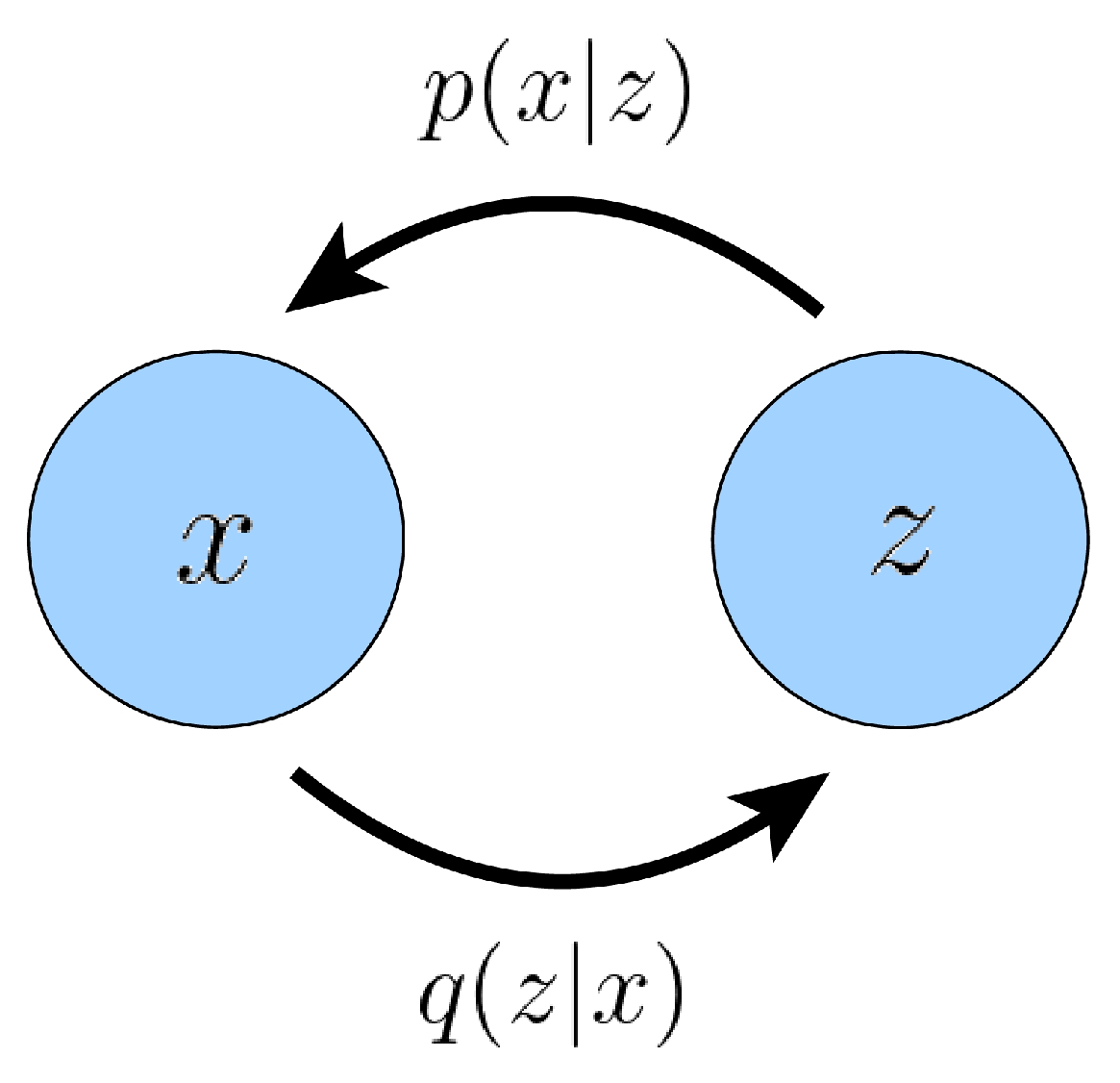
Figure 3.
Score-based generative model. The image shows that the procedure of recovering a high-resolution CT image from noise is gradual.
Figure 3.
Score-based generative model. The image shows that the procedure of recovering a high-resolution CT image from noise is gradual.
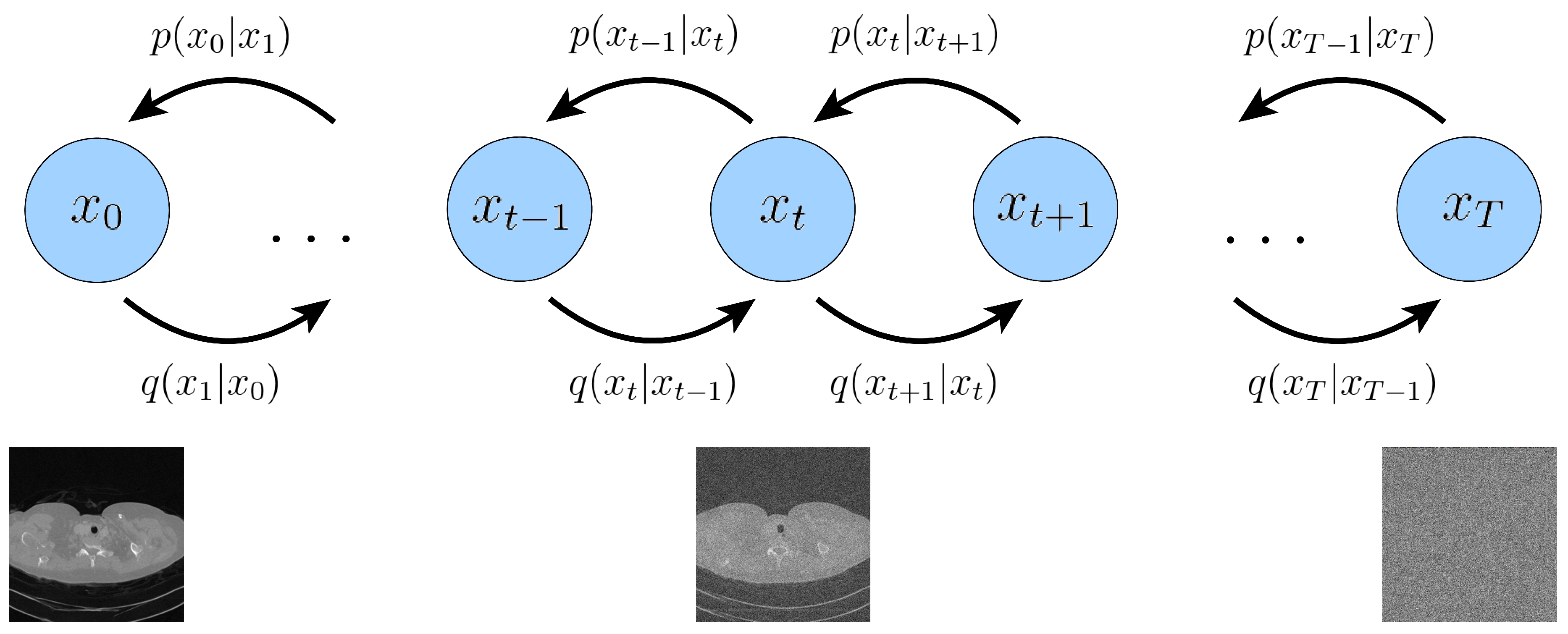
Figure 4.
Three random sampling trajectories generated with Langevin Dynamics, all three starting from the same initialization point, for a mixture of Gaussians. From the same initialization point, we are able to generate samples from different modes due to the stochastic noise term in the Langevin dynamics sampling procedure; without it, sampling from a fixed point would always deterministically follow the score to the same mode each time.
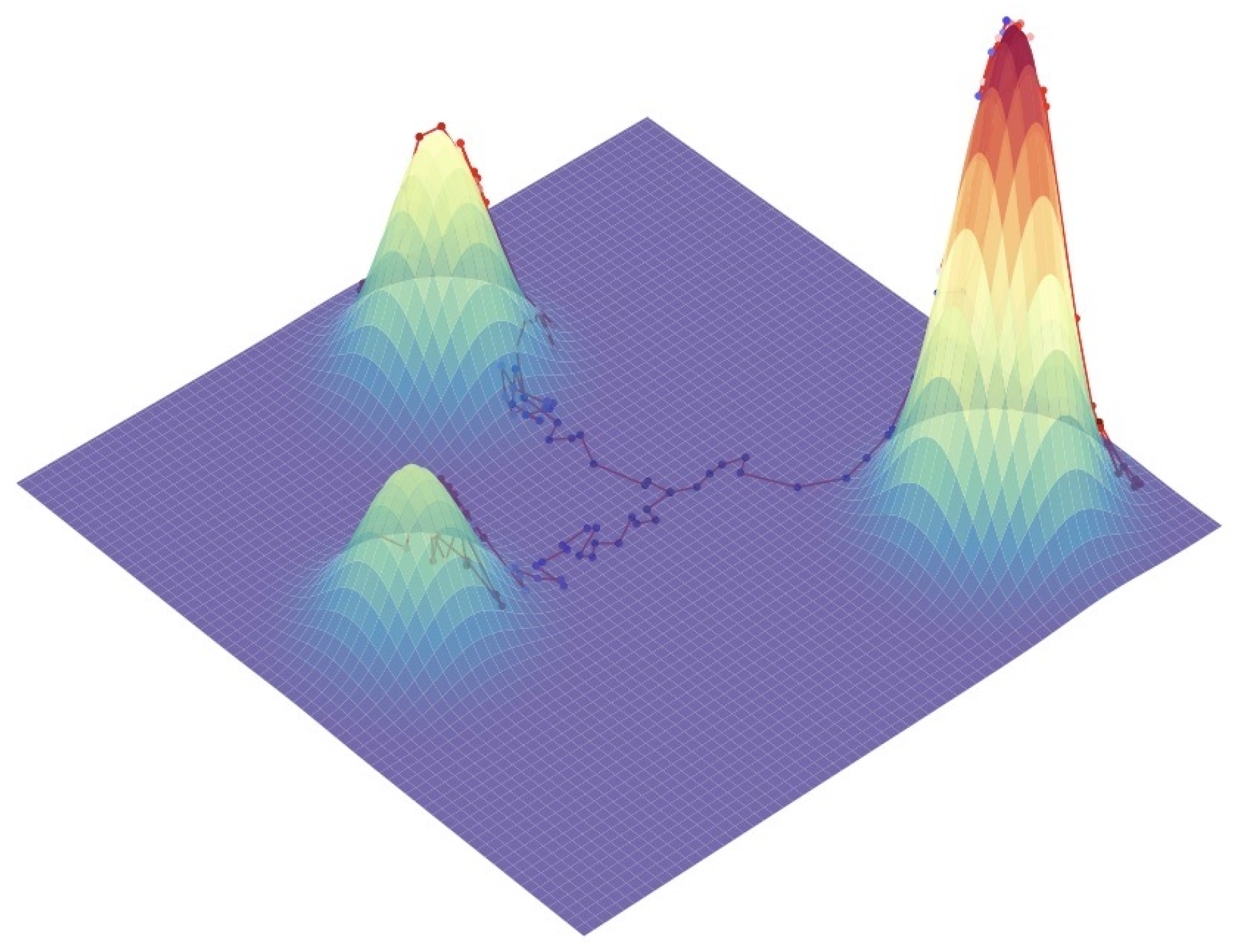
Figure 6.
The reconstruction results of all three methods. From top to bottom, the corresponding are PC-POCS(Proposed), MCG, Song, and the ground truth. PC-POCS has the best performance.
Figure 6.
The reconstruction results of all three methods. From top to bottom, the corresponding are PC-POCS(Proposed), MCG, Song, and the ground truth. PC-POCS has the best performance.
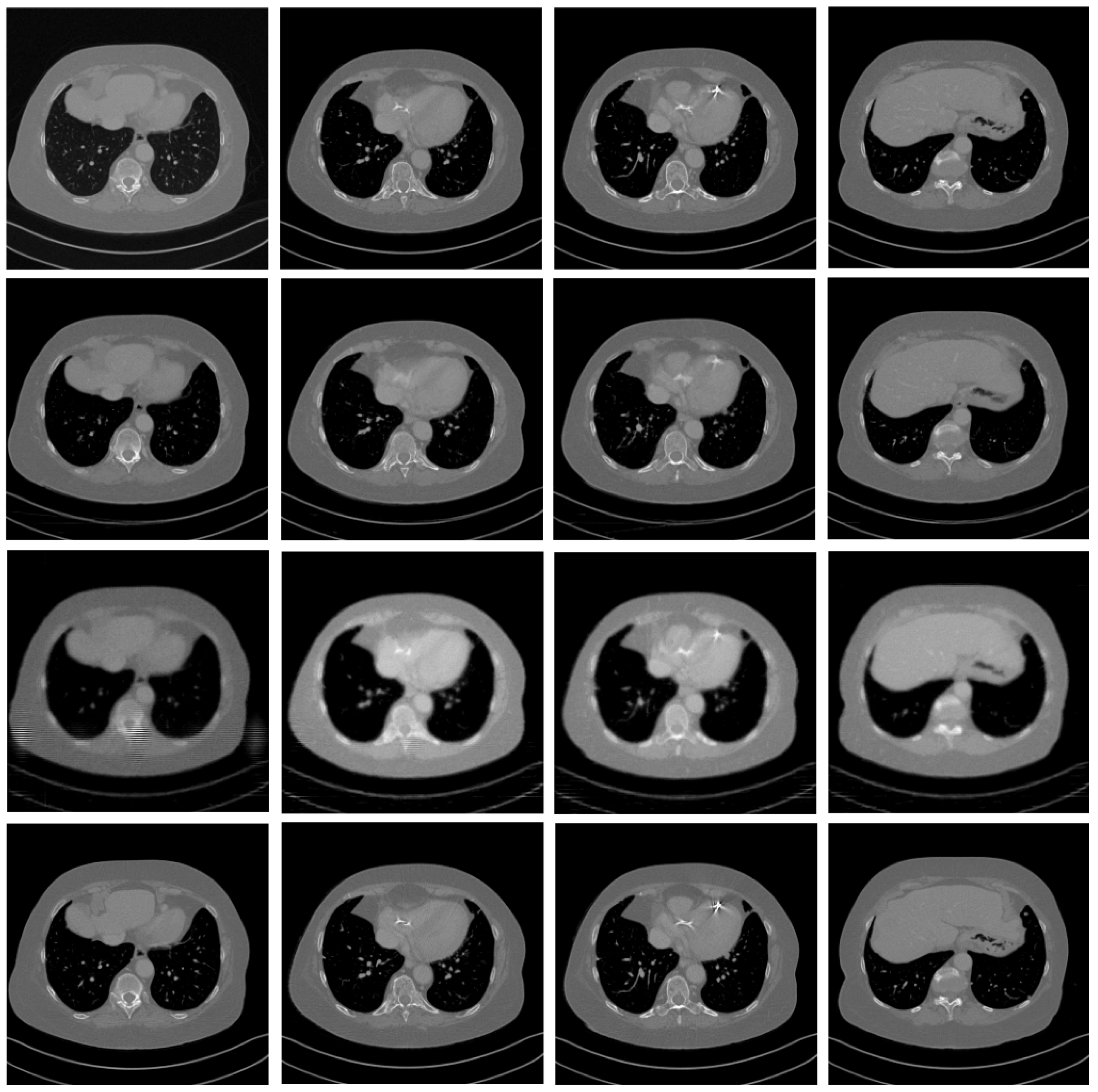

Table 1.
Quantitative results of different methods on AAPM dataset. We experiment on the slice index of . Due to space limitations, we have only presented some of the random results. The Bold characters represent our method. Best numerical results are red; second best are blue.
Table 1.
Quantitative results of different methods on AAPM dataset. We experiment on the slice index of . Due to space limitations, we have only presented some of the random results. The Bold characters represent our method. Best numerical results are red; second best are blue.
| Slice | MCG | Song | PC-POCS | |||||||
|---|---|---|---|---|---|---|---|---|---|---|
| Index | SSIM | FSIM | PSNR | SSIM | FSIM | PSNR | SSIM | FSIM | PSNR | |
| 268 | 0.8245 | 0.8948 | 28.0463 | 0.7534 | 0.8494 | 19.3313 | 0.8902 | 0.9544 | 33.7343 | |
| 269 | 0.8185 | 0.8927 | 27.9395 | 0.7598 | 0.8506 | 19.0324 | 0.8952 | 0.9559 | 34.0099 | |
| 270 | 0.8217 | 0.8935 | 28.1502 | 0.7601 | 0.8489 | 19.8642 | 0.8915 | 0.9550 | 33.7837 | |
| 271 | 0.8265 | 0.9006 | 28.5476 | 0.7555 | 0.8466 | 19.2071 | 0.8886 | 0.9524 | 33.8067 | |
| 272 | 0.8193 | 0.8939 | 27.9205 | 0.7509 | 0.8447 | 19.4014 | 0.8882 | 0.9526 | 33.6799 | |
| 273 | 0.8229 | 0.8978 | 28.2543 | 0.7569 | 0.8447 | 21.0755 | 0.8909 | 0.9531 | 33.6392 | |
| 274 | 0.8124 | 0.8886 | 27.4984 | 0.7603 | 0.8446 | 21.1059 | 0.8867 | 0.9529 | 33.4561 | |
| 275 | 0.8168 | 0.8909 | 27.5838 | 0.7659 | 0.8447 | 23.4483 | 0.8880 | 0.9539 | 33.4843 | |
| 276 | 0.8198 | 0.8914 | 27.4239 | 0.7627 | 0.8461 | 24.8852 | 0.8914 | 0.9544 | 33.4510 | |
| 277 | 0.8141 | 0.8901 | 27.2613 | 0.7693 | 0.8460 | 25.2738 | 0.8868 | 0.9522 | 33.0534 | |
| 278 | 0.8255 | 0.8977 | 27.8815 | 0.7695 | 0.8424 | 24.8828 | 0.8862 | 0.9530 | 33.3379 | |
| 279 | 0.8114 | 0.8894 | 27.2112 | 0.7661 | 0.8481 | 21.6348 | 0.8853 | 0.9530 | 33.3544 | |
| 280 | 0.8231 | 0.9005 | 28.0072 | 0.7706 | 0.8499 | 21.5181 | 0.8867 | 0.9544 | 33.5495 | |
| 281 | 0.8228 | 0.9012 | 27.9217 | 0.7138 | 0.8355 | 23.2376 | 0.8921 | 0.9559 | 33.8156 | |
| 282 | 0.8216 | 0.9021 | 28.4271 | 0.7609 | 0.8478 | 22.7803 | 0.8876 | 0.9558 | 33.7879 | |
| 283 | 0.8263 | 0.9069 | 28.5272 | 0.7701 | 0.8483 | 23.2087 | 0.8881 | 0.9553 | 33.8860 | |
| 284 | 0.8239 | 0.9066 | 28.5368 | 0.7629 | 0.8517 | 25.7797 | 0.8889 | 0.9558 | 33.9643 | |
| 285 | 0.8197 | 0.9007 | 28.3875 | 0.7656 | 0.8554 | 23.0487 | 0.8930 | 0.9567 | 34.2841 | |
| 286 | 0.8274 | 0.9095 | 28.9279 | 0.7659 | 0.7865 | 25.6019 | 0.8927 | 0.9596 | 34.5028 | |
| 287 | 0.8316 | 0.9145 | 29.2608 | 0.7707 | 0.8478 | 21.7916 | 0.8950 | 0.9614 | 34.6276 | |
Disclaimer/Publisher’s Note: The statements, opinions and data contained in all publications are solely those of the individual author(s) and contributor(s) and not of MDPI and/or the editor(s). MDPI and/or the editor(s) disclaim responsibility for any injury to people or property resulting from any ideas, methods, instructions or products referred to in the content. |
© 2025 by the authors. Licensee MDPI, Basel, Switzerland. This article is an open access article distributed under the terms and conditions of the Creative Commons Attribution (CC BY) license (http://creativecommons.org/licenses/by/4.0/).
Copyright: This open access article is published under a Creative Commons CC BY 4.0 license, which permit the free download, distribution, and reuse, provided that the author and preprint are cited in any reuse.


