
Submitted:
24 October 2025
Posted:
27 October 2025
You are already at the latest version
Abstract
Short-read genome assembly still struggles with repeats and sequencing noise, where heuristic graph traversals often misresolve branches and break contigs. Motivated to test a learning-guided approach that scores edges directly on the unitig graph, aiming for more reliable path selection without relying on paired-end or long-read scaffolding, we introduce COGRAM. This graph-learning assembly pipeline integrates a compacted de Bruijn unitig graph with a GCN-guided hybrid search to score edges and reconstruct paths. On Escherichia coli, the method achieves a strong F1 and high global genome coverage, with behavior that varies by local graph complexity: large sampled regions allow the greedy phase to traverse most nodes before beam expansion, yielding high F1; medium-complexity fragments can trap the beam search and truncate recall and coverage; very small regions are trivially solved. These observations motivate practical tuning levers—expanding the greedy horizon, widening the beam, and increasing the top-k retained at branch points—to trade additional computation for robustness. Unlike Eulerian assemblers such as SPAdes, Velvet, and ABySS that combine bubble popping, tip trimming, and paired-end scaffolding to exceed 99\% genome fraction with long, low-error contigs routinely, COGRAM purposefully takes a different route: it poses a Hamiltonian reconstruction on the unitig graph and decodes with a greedy-plus-beam strategy. In early testing, the unitig graph covers 97.9\% of nodes with 94.7\% recall and forms one dominant path, and the model attains approximately 95\% overlap without paired-end or long-read information—evidence that the GCN learns local overlap patterns. Improving contiguity (N50), reducing misassemblies, and lowering base-error rates are deferred to future work; the present results establish COGRAM as a promising proof of concept that bridges learning-based edge inference with classical DBG assembly mechanics.
Keywords:
KMERGENIE
; grid search
; COGRAM
; de Bruijn
; genome assembly
; graph networks
; convolutional networks
; machine learning
; Hamiltonian reconstruction
1. Introduction
Genome assembly is a key task in bioinformatics, but traditional methods can be complex and require specific systems and extensive tuning, making them less accessible for many researchers. De novo assembly reconstructs genomes from raw sequencing reads by building and traversing assembly graphs, but repeats, sequencing errors, and uneven coverage still cause branch ambiguity and contig fragmentation in short-read data. Classical de Bruijn graph (DBG) assemblers such as Velvet, ABySS, and SPAdes address these challenges with graph cleaning (bubble popping, tip trimming) and scaffolding, and routinely deliver high genome fraction on bacterial benchmarks [1,2,3]. Yet, their heuristic path selection can misresolve locally complex regions [2,3].
Long-read HiFi assemblers improve contiguity by using phased assembly graphs and specialized traversals, emphasizing the importance of richer graph signals for path decisions; however, short-read assembly remains widespread and cost-effective, especially for microbial genomes, metagenomes, and legacy datasets [4]. A complementary track improves the substrate graph itself: k-mer spectrum modeling (GenomeScope 2.0/Smudgeplot) informs parameter choices and genome characteristics, and modern compaction algorithms (BCALM 2, CUTTLEFISH 2) shrink graphs to unitigs at population scale [5,6,7].
Early studies suggest that edge multiplicities can help with error correction and repeat resolution, strengthening the case for edge-level inference. Recent research integrates learning directly into assembly graphs. Graph-transformer and geometric deep-learning models score edges or contiguity paths on DBG/assembly graphs, then decode contigs using heuristic traversals, enhancing selection in complex situations, neighborhoods [8,9,10]. On the learning side, Graph Convolutional Networks (GCNs) introduced efficient, locality-aware message passing on graphs, a paradigm now widely adopted to score nodes and edges in biological graphs [11].
Sequence-to-graph alignment has matured with GraphAligner, which delivers fast, versatile mapping of reads to assembly or variation graphs and thus improves polishing, error detection, and structural variant traversal [12]. Systematic benchmarking like GAGE-B highlights performance trade-offs among bacterial assemblers and underscores the need for principled k-mer choice, error handling, and graph traversal policies when evaluating new pipelines against established baselines [13].
We introduce COGRAM (Coggins- Ramasamy Genomic Assembly Method), a Python-native innovative pipeline based on the initial work [14] for genome assembly. It combines principled k-mer selection with compacted de Bruijn unitig graphs and a lightweight graph neural network (GCN) for edge scoring and path reconstruction. This article significantly expands on the conference paper with theoretical derivations, gradient analyses, detailed algorithms, and extended results. Designed for simplicity and portability, COGRAM runs cross-platform without external assemblers (e.g., Velvet [2], SPAdes [1]) or Linux-specific dependencies. It features controlled k-mer sampling for building training sets, unitig compaction that preserves graph structure while reducing size, and a GCN that learns to prioritize true adjacencies from local topology and coverage features. The scored graph is decoded with a greedy-plus-beam strategy, yielding a strong F1 score and high whole-genome coverage on Escherichia coli using only short reads. The behavior reflects local graph complexity: large sampled regions enable the greedy phase to traverse most nodes and achieve high F1 scores.
While medium-complexity fragments can trap the beam, reducing recall and coverage, very small regions reconstruct perfectly. These observations motivate practical tuning levers—extending the greedy horizon, widening the beam, and increasing the top-k at branch points—to trade computation for robustness. Conceptually, k-mers are represented as nodes (one-hot encodings), allowing the model to capture repeat structure and sequence variation without the overhead of conventional assembler pipelines. In aggregate, COGRAM provides a flexible, platform-independent route to accurate segment reconstruction and a controlled test-bed for learning-based methods in genomics. The research questions guiding this work include:
- RQ1:
- How accurately can a GNN reconstruct genomic sequences from real sequencing data?
- RQ2:
- What are the best methods for choosing optimal k-mer values for genome segmentation, and how can these be effectively structured for further analysis?
- RQ3:
- How do different techniques, such as k-mer optimization and graph construction, influence the accuracy and scalability of genome assembly processes?
By answering the above research questions, COGRAM provides a streamlined and innovative framework for genome assembly that bridges the gap between traditional methods and new data-driven approaches.
The remainder of this paper is organized as follows. Section 2 describes the synthesis of related work and foundational concepts and an illustration of optimization and gradient flow in the assembly GNN. Section 3 describes the COGRAM pipeline, including sampling, k-mer selection, unitig graph construction, and GCN training. Section 4 presents the datasets, sampling windows, hyperparameters, and decoding settings. Section 5 reports results on Escherichia coli, including global F1 and genome fraction, as well as per-region recall and coverage, highlighting the dominant-path outcome. Section 6 analyzes the time complexity of the COGRAM framework. Section 7 discusses the results and compares COGRAM with established assemblers using genome fraction, N50, misassemblies, base-error rate, and runtime. It also discusses limitations and practical considerations, including contiguity and error profiles, and outlines optional upstream refinements. Section 8 concludes with implications and future work aimed at increasing contiguity without paired-end or long-read data.
2. Related Work
The problem of genome assembly remains a cornerstone challenge in computational biology, particularly in the context of assembling high-accuracy genomes from short-read sequencing technologies such as Illumina. Given the exponential increase in sequencing throughput and the concurrent complexity of eukaryotic and polyploid genomes, there is a growing need for scalable, accurate, and automated assembly techniques.
Traditional genome assemblers have largely relied on de Bruijn (DBG) frameworks, where reads are fragmented into k-mers, forming a graph whose traversal ideally reconstructs the genome. However, this approach does introduce some nontrivial design choices, such as optimal k-mer length selection and graph simplification heuristics (i.e., pruning of undesired edges while maintaining graph structure balance). These choices have a great impact on the quality of the assembly. Tools such as KmerGenie have provided some probabilistic modeling solutions for k-mer selection, while exploratory data analysis of k-mer distributions and GC-content plots have become commonplace in quality control techniques. Despite these advances, many heuristic approaches remain weak when applied to complex genome regions or data sets with heterogeneous coverage or error profiles.
The field has experienced a boom in the application of ML, and more recently, graph neural networks, to various aspects of genome assembly. These methods offer promise for automated genome assembly, including, but not limited to, automated graph pruning, classification of error-prone edges, and learning assembly traversal directly from data. Early work in this regime has demonstrated impressive gains in contig quality and runtime efficiency - though most are still constrained by reliance on simulated training data or technology specific assumptions like hardware limitations (i.e., parallelized computing to improve graph searching).
2.1. Synthesis of Prior Research
We critically examine six important studies that range from traditional heuristic assemblers to cutting-edge graph network frameworks. We evaluated each study’s methodological structure, highlighted the strengths and weaknesses, and discussed how the approaches intersected or diverged from generalized genome assembly pipelines. We aim to clarify the current state of the field and outline practical and theoretical directions for future work in genome assembly. The methodologies, strengths, weaknesses, and areas of improvement for each of the 6 papers are outlined below.
Genome assembly methods have evolved from parameterized heuristic pipelines toward graph-learning approaches that infer edge validity and path structure directly from data. Early tools emphasized k-mer selection and quality control for short-read de Bruijn graph (DBG) assembly, whereas recent work applies graph neural networks (GNNs) and Transformers to score edges or decode contiguity paths on assembly graphs.
Table 1 summarizes recent studies relevant to genome assembly and graph-learning, listing for each article its focus, data type, graph or model used, core idea, and primary strength to position COGRAM within prior work. Table 2 contrasts traditional de Bruijn–based assemblies with ML-based approaches across key features—k-mer such as optimization, error handling, path selection, evaluation practices, data regimes, and degree of automation to highlight methodological differences and trends.
Collectively, the literature traces a progression from parameter-driven, heuristic DBG pipelines to graph-learning frameworks that infer edge validity and contiguity. Tools such as KmerGenie and empirical k-sweeps established principled parameterization for short-read assembly, while classical pipelines complemented this with QC and contamination checks. GNN-based methods subsequently reframed error handling and traversal as supervised learning on graphs (edge classification or path prediction), and Transformer-based models further extended receptive fields to capture long-range dependencies on HiFi data.
These developments inform the design of COGRAM. By scoring edges on compacted unitig graphs with a lightweight GCN and decoding via a greedy-plus-beam strategy, the approach inherits the portability and simplicity prized in traditional DBG pipelines while leveraging learned signals to resolve ambiguous regions. The result is a balanced, cross-platform method that aligns with the field’s shift toward graph-aware learning without incurring the full computational cost of Transformer-scale models.
2.2. Optimization and Gradient Flow in the Assembly GNN
We begin by recalling the fundamental concepts of how the network assigns labels and its objective: to categorize each edge as 1 (part of the actual ground truth cycle) or 0 (a potential overlap). The standard graph notation employed below is outlined.
- X = input feature matrix of shape
- A = adjacency matrix of the graph.
- In practice, we use to cover self-loops.
- = normalized adjacency matrix, where , is the degree matrix of .
- = trainable weight matrix at layer l. = node embedding matrix after layer l.
After presenting the mathematical details, we will demonstrate a simple example to make the material easier to understand. Each input node i has a feature vector . In the first layer of the GCN, each node i’s new embedding is a weighted average of its neighbors’ features, and then we apply a linear transformation.
This first layer pass gives nodes information about their 1-hop neighbors: Then, the second layer gains information about its 2-hop neighbors: For each edge , we concatenate the node embeddings: , and then pass through a 2-layer MLP, The output logit is passed to a logistic sigmoid to compress to a probability: .
Each GCN layer has a non-linear ReLU (Rectified Linear Unit) activation function , so nodes learn nonlinear combinations of neighbor features. Then at the end, we apply the typical sigmoid to the edge score, compressing it to a probability for training with cross-entropy. The standard binary cross-entropy across edges: and the gradient with respect to logit: which results in a residual: predicted probability minus the truth.
For clarity, note that when backpropagating through nonlinear activations such as ReLU and the edge MLP, the element-wise derivative multiplies each upstream gradient. In other words, for , we have , where ⊙ represents the Hadamard product and .
We now discuss the backpropagation in the context of a graph. At the edge head, each residual updates for the last MLP layer: where . Then we split the residuals back to the nodes following a gradient split of
Each node collects the sum of gradients from all incident edges. For each GCN layer, we define . During backpropagation, if , then For the symmetric normalization used in this work, . Intuitively, just as messages flow forward through neighbors, error signals flow backward through neighbors.
In practice, is symmetric because the unitig graph is treated as undirected during message passing, even though the dedicated edge pairs are later used for classification. This distinction maintains consistency with standard GCN formulations.
2.3. Illustrative Example
Let us consider a simple example to illustrate how this process operates using real data. Suppose we have a mini graph represented using the following adjacency matrix:
We add self-loops: , therfore, ,
The degrees of .We then complete the GCN normalization (the full details of which are omitted for the sake of real estate and preserving the reader’s eyes and attention). Numerically we use and
Let’s take a tiny 2-dimensional input: where, row .
In the real model, X is a flattened 4 x k one-hot vector per node. In layer 1, . We pick for simplicity, and is just a ReLU. First, compute (row-by-row):
- Row 1: 0.5[1,0] + 0.4082[0,1] = [0.5, 0.4082]
- Row 2: 0.4082[1,0] + 0.3333[0,1] + 0.4082[1,1] = [0.8164, 0.7415]
- Row 3: 0.4082[0,1] + 0.5[1,1] = [0.5, 0.9082]
Each node mixed its own feature (self-loop) with its neighbors’ features, normalized by degree. In layer 2, . We again choose to isolate the effect of . Now, compute each
- Row 1:
- Row 2:
- Row 3:
Now each node encodes a 2-hop structure. For the edge scoring (how the head uses , given a directed edge , we build the edge feature by concatenation:
Then we apply a small MLP (or single layer for simplicity): and we train with BCE: That residual back-propagates into and , and then through the GCN layers via - so errors also message-pass over the graph during learning.
We want to clarify for the reader that "big" is the matrix form (all nodes at once) and "little" is the vector form of a single node. More compactly for the mathematically inclined readers: denotes the matrix of all node embeddings at layer l, where each row corresponds to node i. We also note that this mathematical treatment extends standard GCN theory to genome graphs.
3. Overview of the COGRAM Framework
In this section, our goal is to outline a birds-eye view of the COGRAM model, and then fly down to the ground level and discuss each component of the framework. Figure 1 shows the end-to-end COGRAM pipeline—from FASTA sampling and k-mer optimization to unitig de Bruijn graph construction, GCN training, and greedy-plus-beam decoding—culminating in global and region-level metrics. Algorithm labels (1–6) mark the procedure used at each stage, and arrows indicate the data flow and the feedback of pickled graph data and model checkpoints into evaluation.
3.1. Sampling Process
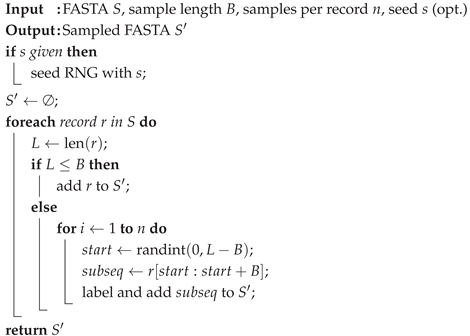
For each chromosome in the input FASTA, Algorithm 1 shown below randomly samples one or more contiguous windows of a specified length (for example, 10000). This is critical because working with full chromosomes will dramatically slow down the development and testing of the pipeline. Using lightweight “mini" chromosomes allows us to iterate through the pipeline quickly for testing.
| Algorithm 1: SampleSubsequences |
 |
3.2. Optimization of K-value Selection
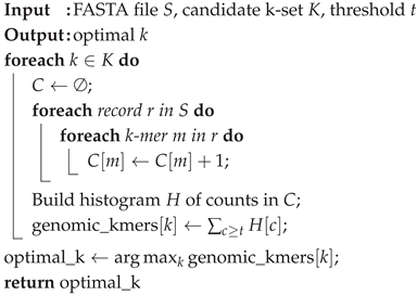
Instead of relying on other assemblers or models like KMerGenie that require a Linux-based system, we have constructed a new, naive optimizer (Algorithm 2). This new optimizer scans over a range of k-values, counts the k-mer abundances, filters out singletons, and picks the k whose "genomic" k-mer count (abundance ≥ threshold) is maximal. It then plots the estimated genomic k-mer counts vs. k, saves the figure, and writes the chosen k-value to a .txt.
| Algorithm 2: SelectOptimalK |
 |
Picking the correct k-mer length is critical for building a reliable de Bruijn graph downstream in our pipeline. If k is too small, there will be too many repeated k-mers, and if k is too large, the graph may become fragmented and harder to navigate (lower connectivity).
We will discuss more of the results in the next section, showing how we arrive at reasonable, sampled FASTA data for the development of this pipeline. The FASTA format is a text-based format for representing either nucleotide sequences or amino acid (protein) sequences, in which nucleotides or amino acids are represented using single-letter codes [19].
3.3. Data Processing
Algorithm 3 is used to transform the sampled FASTA data into two objects: (i) A raw k-mer overlap graph for network training, and (ii) A unitig-compressed graph for faster assembly.
| Algorithm 3: BuildAndCompressGraph |
| Input: Sampled FASTA S, k-mer size k, prefix p Output: Pickles: , Extract overlapping k-mers → N, order O; Build raw edges by -overlap on N; Label true edges in via O; Compute one-hot features F Save raw graph ; Compute unitig mapping ; Aggregate features/labels per unitig → ; Save unitig graph ; |
To clarify our terminology here, we define a contig to be a continuous stretch of DNA sequence reconstructed by an assembler. When an assembler stitches together reads to build as long a sequence as possible without ambiguities or unresolved repeated patterns, we arrive at the contig. By contrast, a unitig is a maximal non-branching path in a de Bruijn graph, collapsed into a single node. The following simple steps describe the process:
- (i)
- Build a DBG whose nodes are k-mers and edges connect overlapping k-mers.
- (ii)
- Wherever a node has exactly one edge in and one edge out (i.e., no branching), we merge them. [Note: This specific step makes an assumption that will be discussed later on in the conclusion.]
- (iii)
- Repeat steps (i) and (ii) until every remaining node has either >1 in-edge or >1 out-edge.
Unitigs are unambiguous, meaning there is exactly one path through them. This is very useful in reconstruction because it enables us to traverse a large section of the graph quickly. In other words, the raw graph maintains granularity for training the model. At the same time, the unitig significantly reduces the graph size by several orders of magnitude by collapsing linear chains into a single node.
3.4. Exploratory Data Analysis
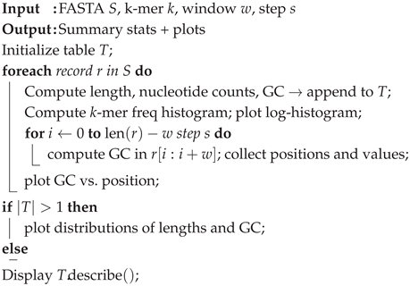
The EDA step (Algorithm 4) serves to inspect our data and ensure that what we are working with is of acceptable quality. We do this by examining two main features: the k-mer frequency abundance and the GC content window. For each record, we compute the length, A/C/G/T counts, and overall GC content and append it to a list for a DataFrame in pandas. We compute the k-mer frequency and plot it on a log scale (because we are dealing with hundreds of thousands), and then compute the GC sliding window to visualize what portion of the record, as a percentage, contains either guanine or cytosine. This content is well-studied and provides us with insight into the stability of the genome.
| Algorithm 4: PerformEDA |
 |
Aside from genome stability, a good data analysis allows us to catch uncharacteristic behaviors such as wild GC fluctuations, contamination in the genome, and just allows us to be comfortable with our input data.
3.5. GCN Training
The purpose of the training, is for our model to learn how to predict which edges in the raw k-mer graph correspond to a true sequence, or ground truth cycle. In other words, our model is an edge classifier. Algorithm 5 outlines the edge-classifier training workflow, from loading the pickled graph and creating PyG data through stratified edge splits and model initialization, to epoch-wise optimization with validation, checkpointing and early stopping, and final evaluation of the best checkpoint.
| Algorithm 5: TrainEdgeClassifier |
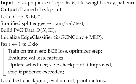 |
This is the heart of our machine learning approach - teaching a graph neural network to recognize real adjacencies versus spurious overlaps in the graph. Once the graph is loaded in, the graph data is split into a training, validation, and testing set with a 70/15/15 split. The model clearly defines an edge classifier: two GCN layers to embed each node, then an MLP that takes a pair of node embeddings and outputs a score for the edge. It then runs a standard deep-learning training model with BCE loss, Adam optimizer, learning-rate scheduling, and early stopping - and then saves the best model.
3.6. Assembly Analysis
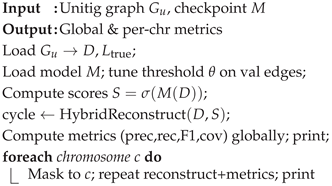
Our model imposes a hybrid reconstruction technique to pass through the unitig graph and the best model checkpoint, and then reconstruct the original sequence as best as we can. This is our assembly validation step, which measures real-world performance on both a global scale and chromosome-by-chromosome performance (Algorithm 6).
- Tune an edge-score threshold for the best validation F1.
- Reconstruct the Hamiltonian cycle with a greedy/beam hybrid that respects branches.
- Report precision, recall, F1, and coverage globally and per "chromosome"
We use the term “chromosome" lazily here, as it refers to a sample region, not an actual biological chromosome. The reconstruction is a two-stage reconstruction, wherein the greedy walk takes the highest scoring edges until we’ve recovered a user-defined fraction of the nodes. After the greedy walk, we swap to a branch-aware beam search at branch points, saving top candidates, gluing in the rest of the cycle.
| Algorithm 6: EvaluateAssembly |
 |
4. Experimental Setup
To begin, our datasets are gathered from the NIH genome database[20].These datasets are clean and ready for work, since FASTA data can be downloaded directly. For initial testing, we chose E. coli, since it is such a short genome and only contains one biological chromosome. This dataset is approximately 4 Mb, which makes for very manageable sampled graphs.
The model architecture has two hyperparameters: in channels set the dimensionality of the input features. In our case, we choose 4 x k for one-hot encoded k-mers. For example, A is encoded to [1,0,0,0]. The hidden channels are set to 32, which is the size of each GCN embedding layer. As the hidden layers are adjusted, we can monitor various F1 values during validation. The edge multi-layer perceptron (MLP) has two linear layers:
- First layer maps for concatenated source and target embeddings.
- Second layer maps for edge logits.
For the training hyperparameters, we will start with epochs. This is a standard value, currently set to 100 for the maximum training passes. However, the model tends to stop around 70 epochs for this particular dataset since we have implemented early-stopping conditions to prevent wasted epochs. If the validation loss does not improve for 10 epochs, the training will stop. If validation plateaus too early in the training, we can adjust the learning rate for the Adam optimizer. We also have implemented a scheduler to dynamically cut the learning rate by a factor of 1/2 if the validation loss does not improve for 5 epochs.
For reconstruction, we can control the greedy fraction, the beam width, and the top scoring edges at each branch for expansion. A larger greedy search fraction speeds up the reconstruction substantially, but we lose global exploration if it is too high. Too small, and we risk entering beam search too early, which is substantially higher compute load. The beam width is in initially set to 3 to check 3 candidate paths, and we keep the top 5 highest-scoring outgoing edges at each iteration of the beam expansion. This hybrid reconstruction algorithm speeds things up substantially while still allowing us to traverse a very large portion of the genome.
To fine-tune training, we’d need to sweep over several greedy fractions in the interval of [0.1, 0.3, 0.5]. For each sweep of the greedy fractions, we also sweep over beam width and top k values: (3,5), (5,10), (10,20). While these sweeps are occurring, we plot F1 score and runtime for each configuration and then choose a preferred regime.
The test hyperparameter settings include: k = 21, Number of samples = 5, Epochs = 100, Learning Rate = 0.01, Weight Decay (for L2 regularization) = 1e-4, Patience = 10, Greedy Fraction = 0.3, Beam Width = 5, and Top K = 10. All training took place on an RTX 3070 and lasted about 15 minutes. It is worth noting that we get away with very fast training because our graph is very small for this particular genome. Moving to larger genomes would require fine-tuning the model more (which is discussing in shortcomings).
5. Preliminary Results
Since we only tuned our network for very specific values, we only have one set trained on with some validation completed. We will discuss the hyperparameter settings and findings in this section.
5.1. K Optimization
We look at the k-mer distribution of one of the samples here since they are all virtually the same in this set-up. According to the figure below, we choose k = 21 (Figure 2).
5.2. Data Analysis
Since the K-mer frequency distribution was nearly identical for all samples, we present the results of K-mer frequency abundance for samples 1-5 in Figure 3.
The large peak at 1.0 indicates that the overwhelmingly vast majority of the k-mer segments are unique. The small peak at 2.0 means that there are some duplicates, but very few by comparison. The GC-content window for all samples is also shown here. Having all GC-content near 50% for all samples indicates standard amounts based on biological genome samplings (Figure 3 - Bottom-Right).
5.3. Reconstruction and Validation
After training and reconstruction using our hybrid algorithm, we arrive at the following results for our initial passes. On a global view of the genome, the results include: Precision = 0.967, Recall = 0.947, F1 = 0.957, and Coverage = 0.979.
Our precision score indicates that of all edges our reconstruction predicted as ground-truth, 96.7% actually were true adjacencies. The recall indicates that of all the true edges in the unitig graph, we recovered 94.7% of them. The harmonic mean (F1) yields a strong overall performance, and 97.9% of the nodes were visited at least once in the reconstructed cycle.
The confusion matrix is given as
The description of the confusion matrix entries, True Positive (TP), True Negative (TN), False Positive (FP), and False Negative (FN) and their meaning are summarized below.
- TN = 165: edges correctly predicted as non-existent (very few, since non-edges vastly outnumber real edges)
- FP = 12,059: edges predicted as real when they weren’t - reflecting some class imbalance.
- FN = 80: true edges the cycle failed to include.
- TP = 6,776: true edges correctly recovered
We can also examine per-chromosome (sampled regions) scores given in Table 3.
Large windows perform best: Sample 2 achieves high precision (0.986), recall (0.961), F1 (0.973), and coverage (0.975) because the greedy phase already visits a large fraction of nodes (1193/3977), leaving little for the beam to resolve. Trivial windows collapse perfectly: Sample 5 needs no beam and hits 1.000 on all metrics. Samples 3–4 (medium complexity) show high precision (0.929/0.967) but low recall (0.580/0.535), depressed F1 (0.714/0.689), and lower coverage (0.626/0.553) when the beam makes no expansions and stops. This indicates stalls rather than mislabeling—predictions are accurate when taken, but exploration is curtailed. Sample 5 is trivial and perfect (all 1.000), while Sample 1 is intermediate with limited greedy coverage and middling recall/F1—indicating the main fix is to extend the greedy horizon and widen the beam/top-k in medium regions.
6. Time Complexity Analysis of COGRAM Framework
To break down each of the asymptotic costs for the main five algorithms (excluding the data analysis), let’s use the following notations for convenience:
- N = total number of de Bruijn graph nodes (k-mers or unitigs)
- E = total number of graph edges
- L = total number of bases in the input FASTA
- K = number of k-values tested (only applies to k-mer optimization)
- T = number of training epochs
- H = hidden dimensionality of GCN
- B = (treated as a constant)
- C = number of chromosomes
6.1. Sample FASTA (Algorithm 1)
For each of R input records of length : If maxbases, we use a constant; otherwise, we take several samples, random windows of length maxbases; each substring copy is . Then we write out sampled bases. This gives an overall time complexity of .
6.2. Naive k-mer Optimizer: (Algorithm 2):
For each k-value swept over, we parse the entire FASTA of total length L, and for each position, extract one k-mer and update a counter: and build an abundance histogram over at most unique k-mers. We find the optimal k value by scanning over K entries, and then plot and save , which is negligible. Therefore, we have a time complexity of .
6.3. Building the Graphs (Algorithm 3):
This algorithm is broken down into several steps.
- Process chromosomes (per record of length n): Slide window to extract all k-mers:
- Build a prefix map over N nodes: . For each node, look up all matching suffixes - this is a worst case of , where m is the average prefix bucket size; more typically .
- Label the ground trugh edges by marking true edges:
- Compress unitigs: Build in/out adjacency: . Walk each node and collapse the chains: . Rebuild unitig edge set by scanning the edges: .
- Label assembly: .
Overall, this results in a time complexity of . If every single k-mer overlaps, then it is , but this does not happen in practice.
6.4. Train the Model (Algorithm 5):
We break down the training into several steps:
- Data Loading and Splitting:
-
Per-epoch training:
- (a)
- Forward pass: two GCN layers over E edges + MLP edge scoring:
- (b)
- Backwards pass: similar cost
- (c)
- Evaluate on train and validation splits: two more forward passes: .
- (d)
- Total per epoch: .
- Total training: .
- Post-training plots: .
Overall time complexity: .
6.5. Assembly Analysis(Algorithm 6):
We break down this process into several steps as well:
- Data Loading & Model setup: .
- Threshold tuning requires two components: a forward pass of the GNN over all edges: and sweep 81 thresholds, computing F1 on the validation split each time: .
-
Branch-Aware Cycle reconstruction:
- (a)
- Score computation: one forward pass, .
- (b)
- Adjacency build: .
- (c)
- Greedy Phase: up to steps; at each step sort a constant-size neighbor list: (We be lazy and let , which is close to true values).
- (d)
- Beam Phase: up to iterations; each expands ≤ B paths over degree d neighbors: (if d is small).
- (e)
- Total reconstruction: .
- Per-chromosome evaluation: For each chromosome, mask/filter E edges and re-run cycle evaluation. Since C is generally small, this is the same as total reconstruction.
Thus, the overall algorithm is . Even though we use a Hamiltonian cycle approach, our pipeline still runs in polynomial time, scaling with the size of the dataset.
7. Discussion of Results
Overall, we have a strong F1 score and coverage of the global genome. However, when examining the sampled regions, we can see some very different results. Large samples, such as sample 2, let the greedy search cover most of the nodes before the beam, yielding a high F1. Medium complexity fragments are perhaps the most interesting: These are samples 3 and 4, because the beam search appears to become trapped, which cuts off recall and coverage entirely since it cannot expand farther. Small samples are quite dull, since they’re trivial and return perfect results because the search space is very small.
For samples where the beam prematurely fails, we should increase the greedy search to cover more of the nodes. We could also widen the beam and/or raise the top k value kept at branch points to consider more candidate edges, at the expense of compute power.
When compared with other state-of-the-art tools like SPAdes, Velvet, or ABySS, our pipeline differs slightly and gives slightly lower results. These tools take FASTA reads, build k-mer graphs, and then find an Eulerian path through the graph in polynomial time. They then resolve bubbles, perform tip-removal, and scaffold contigs with paired-end information. These tools typically achieve > 99% accuracy of the genome in large, continuous scaffolds with very few misassemblies.
Our model differs in a few key manners:
- Hamiltonian vs. Eulerian: Our model solves a Hamiltonian cycle problem and then reconstructs using a hybrid algorithm.
- Scale and contiguity: Our unitig graph covers 97.9% of the nodes with 94.7% recall, but we have one large path rather than a set of error-free contigs with N50 measured in the tens or hundreds of kilobases.
- Proof of concept: Achieving 95% overlap without any paired-end or long-read information is promising - it demonstrates the GCN can learn local overlap patterns.
In a DBG, a bubble is a pair of divergent paths that start and end at the same nodes - often caused by sequencing errors. Assemblers identify bubbles by finding these “bulges" and then remove the lower-coverage branch, thereby “popping" the bubble and restoring a linear path. A tip of a dead-end branch is a path that doesn’t reconnect. This typically is caused by low frequency k-mers or errors in assembly. Assemblers trim tips shorter than a coverage of length threshold to avoid spurious contigs. Finally, scaffolding with pair-end reads uses known insert-size and orientation of paired reads to link contigs. If two reads in a pair map to different contigs, their distance and direction constraints can order and orient those contigs into scaffolds, bridging gaps that the typical DBG construction cannot resolve.
Table 4 above provides the following key information.
- Genome Fraction: The % of the reference covered by assembled contigs.
- N50: contig length such that 50% of the assembled bases are in contigs greater than or equal to the length.
- Misassemblies: structural errors
- Base Error Rate Mismatch + indel label errors in the consensus.
We plan to tackle the N50, Misassemblies, and Base Error Rate at a later date. For now, we note to the reader that our genome fraction is 97.9 %, which is wonderful for early testing.
8. Conclusion and Future Directions
Overall, the initial version of the test model was successful and demonstrated excellent reconstruction and training on a very small set. In the immediate future, we can refine training parameters and sweep over various regimes outlined in Section III. Long term, we can attempt end-to-end de novo assembly and compare the results to other assemblers.
We note that there are some shortcomings of this model, such as the naive k-mer optimizer. Sweeping over a range of k-values starting at might lead to very consistent results, regardless of the genome being checked. For example, E. coli and yeast may yield the same optimal k-value, but this may not be true due to the varying complexity of the nucleotide sequence. We can remedy this by taking some techniques inspired by [15], by fitting a two-component mixture to the abundance histograms (error vs genomic). Then pick the k that maximizes the estimated number of high-abundance.
Additionally, finding the assembly as a Hamiltonian cycle on the unitig graph is elegant, but very computationally expensive, as it is known to be NP-hard. The beam search portion is heuristic and has no guarantees. Additionally, we have no explicit error-correction or graph cleaning. Real assemblers prune low-coverage trips, pop bubbles, and remove spurious branches. This results in a brittle and hyperparameter-sensitive approach. It can be resolved by reverting to an Eulerian assembly with graph simplification.
Furthermore, we must note that the “compactifying" of the graph during the graph building algorithm has an assumption that must be addressed. There is no guarantee that every raw edge in the compressed node was part of the ground-truth cycle since the labeling doesn’t happen until after compression. In practice, spurious (label = 0) overlaps tend to create branching, so maximal unbranched chains likely do reflect the true sequence. However, this is heuristic and not an enforced variant. This will be addressed in future work.
The overall goal was to construct a pipeline that is system independent (i.e., without the need for Linux-based assemblers like Velvet or SPAdes) and easy to tune. The system needs extensive testing with other datasets and hyperparameter tuning, but offers promising initial results. The ideas outlined in this paper provide a versatile GNN framework that can be taken in two practical directions: (i) Error Detection in Genome Sequencing for Disease Diagnostics, and (ii) Social-Network Analysis. For direction 1, we frame the problem as looking at low-coverage regions and structural variants that often show up as “anomalous" patterns in the DBG - such as extra branching, bubbles, or dead-ends that don’t follow the main path. The pipeline can be adapted by training on a mix of high-confidence truth data and simulated errors (e.g., inducing sequencing mistakes for known pathogenic variants). The GNN classifier could learn to flag edges that are likely sequencing errors or variant breakpoints. Once flagged, we can isolate the “bubbles" in the graph, realign the reads locally, and compare with structural variants linked to disease loci. This could even be trained on patient-specific data to flag pathogenic variants in long-read or single-cell protocols.
For direction 2, we examine social graphs where users are nodes and interactions are edges, that share the same “link-prediction" and “community-structure". We propose replacing the k-mer one-hots with user demographics, activity patterns, text embeddings, etc. Instead of ground truth adjacency labels, we can label edges as trusted/fraudulent, likely friendships, or information cascade paths. We then train the GNN to predict edges that will form in the future, or latent ties that were not explicitly recorded. It could also help identify fake accounts or bot networks by identifying structurally inconsistent edges. The potential applications of this are fraud detection, recommender systems, and epidemiology of memes.
At its heart, this research project is based on future-driven edge classification and hybrid path reconstruction. The pipeline is a ready-made scaffold for both of the above domains that require careful labeling and feature engineering, but leverage the same architecture and logic.
Author Contributions
Conceptualization, W. Coggins and V. Ramasamy.; Methodology, W. Coggins and V. Ramasamy; Programming, W. Coggins.; Validation, W. Coggins and V. Ramasamy; Formal Analysis, W. Coggins; Investigation, W. Coggins; Resources, W. Coggins and V. Ramasamy; Data Curation, W. Coggins; Writing—original draft preparation, W. Coggins; Writing—review and editing, W. Coggins and V. Ramasamy; visualization, W. Coggins and V. Ramasamy; Supervision, V. Ramasamy; Project Administration, V. Ramasamy.; funding acquisition (travel) Not applicable. All authors have read and agreed to the published version of the manuscript.
Funding
The research is not funded.
Institutional Review Board Statement
Not applicable.
Informed Consent Statement
Not applicable.
Data Availability Statement
All data obtained for this manuscript are from [20] and are readily available to download publicly. All code for this research is in the process of being updated and maintained on GitHub and will also be publicly available after the completion of the research.
Acknowledgments
During the preparation of this manuscript the author(s) used Mermaid to generate the Figure 1. The authors have reviewed and edited the output and take full responsibility for the content of this publication.
Conflicts of Interest
The authors declare no conflicts of interest.
Abbreviations
The following abbreviations are used in this manuscript:
| MDPI | Multidisciplinary Digital Publishing Institute |
| DOAJ | Directory of open access journals |
| DBG | De Bruijn Graph |
| GNN | Graph Neural Network |
| GCN | Graph Convolution Network |
| EDA | Exploratory Data Analysis |
| COGRAM | Coggins-Ramasamy Assembly Method |
References
- Bankevich, A.; Nurk, S.; Antipov, D.; Gurevich, A.A.; Dvorkin, M.; Kulikov, A.S.; Lesin, V.M.; Nikolenko, S.I.; Pham, S.; Prjibelski, A.D.; et al. SPAdes: A New Genome Assembly Algorithm and Its Applications to Single-Cell Sequencing. Journal of Computational Biology 2012, 19, 455–477. [CrossRef]
- Zerbino, D.R.; Birney, E. Velvet: algorithms for de novo short read assembly using de Bruijn graphs. Genome Research 2008, 18, 821–829. [CrossRef]
- Simpson, J.T.; Wong, K.; Jackman, S.D.; Schein, J.E.; Jones, S.J.; Birol, A. ABySS: a parallel assembler for short-read sequence data. Genome Research 2009, 19, 1117–1123. [CrossRef]
- Yu, W.; Luo, H.; Yang, J.; Zhang, S.; Jiang, H.; Zhao, X.; Hui, X.; Sun, D.; Li, L.; Wei, X.Q.; et al. Comprehensive assessment of 11 de novo HiFi assemblers on complex eukaryotic genomes and metagenomes. Genome Research 2024, 34, 326–340. [CrossRef]
- Ranallo-Benavidez, T.R.; Jaron, K.S.; Schatz, M.C. GenomeScope 2.0 and Smudgeplot for reference-free profiling of polyploid genomes. Nature Communications 2020, 11, 1432. [CrossRef]
- Chikhi, R.; Limasset, A.; Medvedev, P. Compacting de Bruijn graphs from sequencing data quickly and in low memory. Bioinformatics 2016, 32, i201–i208. [CrossRef]
- Khan, J.; Kokot, M.; Deorowicz, S.; Patro, R. Scalable, ultra-fast, and low-memory construction of compacted de Bruijn graphs with Cuttlefish 2. Genome Biology 2022, 23, 190. [CrossRef]
- Luo, J.; Fang, H.; Xie, L.; Wang, Y.; Gao, X. GTasm: A genome assembly method using graph transformers and HiFi reads. Frontiers in Genetics 2024, 15, 1495657. [CrossRef]
- Vrček, L.; Bresson, X.; Laurent, T.; Schmitz, M.; Kawaguchi, K.; Šikić, M. Learning to Untangle Genome Assembly with Graph Convolutional Networks, 2022, [arXiv:q.bio.GN/2206.00668].
- Vrček, L.; Bresson, X.; Laurent, T.; Schmitz, M.; Kawaguchi, K.; Šikić, M. Geometric deep learning framework for de novo genome assembly. Genome Research 2025, 35, 839–849. [CrossRef]
- Kipf, T.N.; Welling, M. Semi-Supervised Classification with Graph Convolutional Networks. 2016, [arXiv:cs.LG/1609.02907].
- Rautiainen, M.; Marschall, T. GraphAligner: Rapid and versatile sequence-to-graph alignment. Genome Biology 2020, 21, 253. [CrossRef]
- Magoč, T.; Pabinger, S.; Canzar, S.; Liu, X.; Su, Q.; Puiu, D.; Tallon, L.J.; Salzberg, S.L. GAGE-B: an evaluation of genome assemblers for bacterial organisms. Bioinformatics 2013, 29, 1718–1725. [CrossRef]
- Coggins, W.; Ramasamy, V. Computational Pipeline for Genome Assembly and Reconstruction via Optimized K-mer Sampling and De Bruijn Graph Networks. In Proceedings of the Proceedings of the 17th International Conference on Advances in Social Networks Analysis and Mining (ASONAM 2025), Canada, August 2025. To appear.
- Chikhi, R.; Medvedev, P. Informed and Automated k-mer Size Selection for Genome Assembly. Bioinformatics 2014, 30, 31–37. [CrossRef]
- Cha, S.; Bird, D.M. Optimizing k-mer size using a variant grid search to enhance de novo genome assembly. Bioinformation 2016, 12, 36–40. [CrossRef]
- Duan, Y.; Li, Y.; Zhang, J.; Song, Y.; Jiang, Y.; Tong, X.; Bi, Y.; Wang, S.; Wang, S. Genome Survey and Chromosome-Level Draft Genome Assembly of Glycine max var. Dongfudou 3: Insights into Genome Characteristics and Protein Deficiencies. Plants 2023, 12. [CrossRef]
- Simunovic, M.; Vrcek, L.; Sikic, M. Graph Neural Network Meets de Bruijn Genome Assembly. In Proceedings of the 2023 International Symposium on Image and Signal Processing and Analysis (ISPA), 2023, pp. 1–6. [CrossRef]
- Lipman, D.J.; Pearson, W.R. Rapid and sensitive protein similarity searches. Science 1985, 227, 1435–1441. [CrossRef]
- NIH Library of Medicine. Genome Library, 2022. https://www.ncbi.nlm.nih.gov/datasets/genome/.
Figure 1.
COGRAM Framework
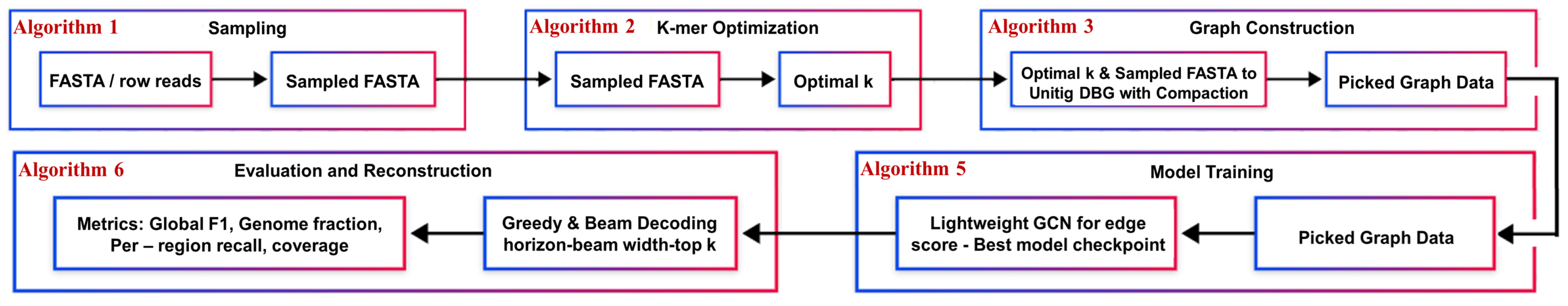
Figure 2.
Naive K-mer Optimization

Figure 3.
K-mer Frequency Abundance for Samples 1–5. and Frequency Distribution of GC Across 5 Samples (Bottom-Right)
Figure 3.
K-mer Frequency Abundance for Samples 1–5. and Frequency Distribution of GC Across 5 Samples (Bottom-Right)
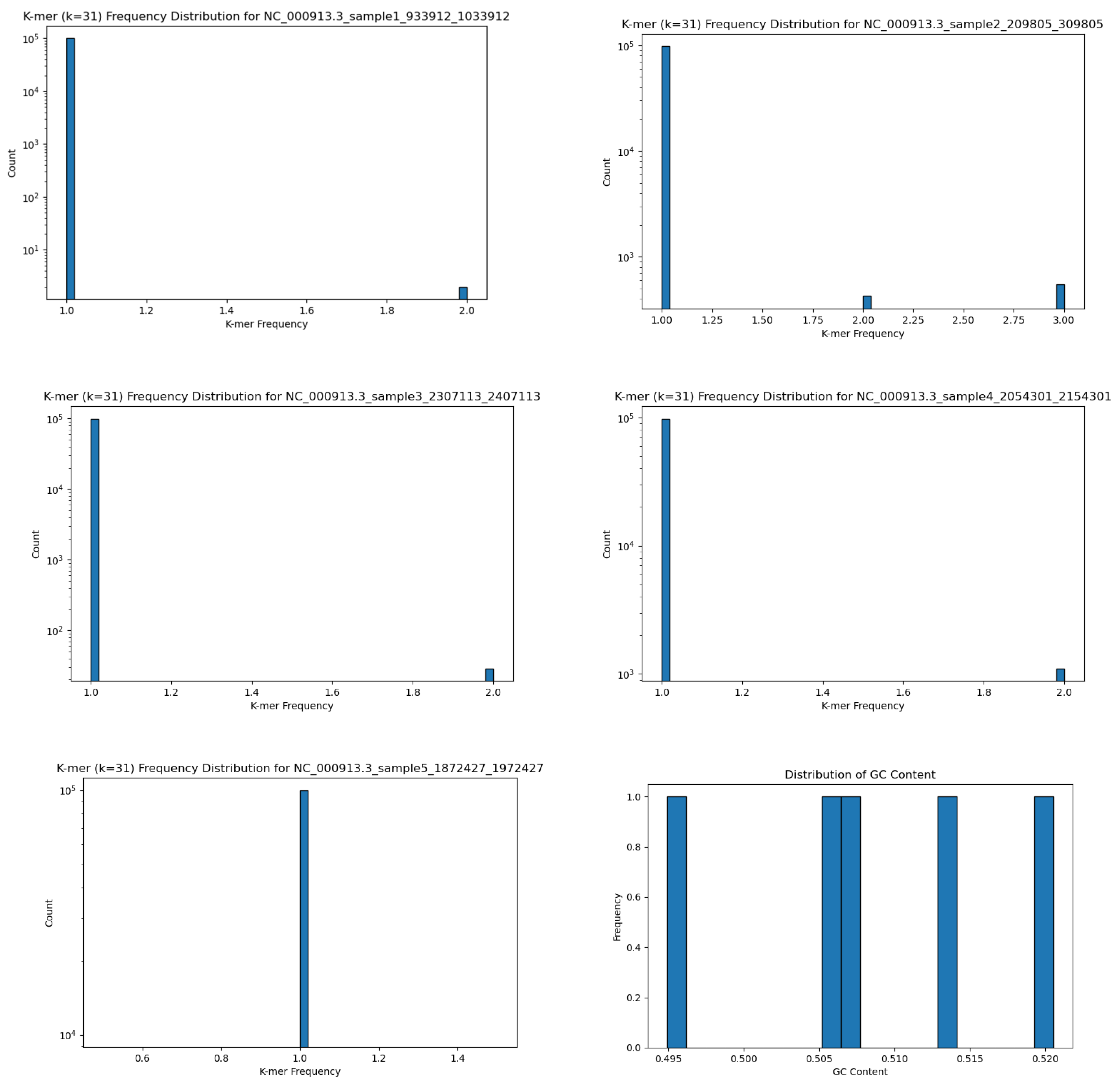

Table 1.
Overview of selected studies in genome assembly and graph-learning for assembly.
| Article | Focus | Data | Graph/Model | Core Idea | Strength |
|---|---|---|---|---|---|
| Chikhi & Medvedev 2014 [15] | k-mer size selection | Short reads | Histogram model | Estimates “solid” k-mers to pick optimal k | Automates parameter choice |
| Cha & Bird 2016[16] | Empirical k grid search | Short reads | Heuristic sweep | Tests multiple k using N50/CEGMA | Simple, reproducible tuning |
| Zhang et al. 2023[17] | Classical DBG + EDA | Short reads | SOAPdenovo + QC | Integrates contamination and reference checks | Strong quality control |
| Simunović et al. 2023[18] | GNN edge classification | (Sim.) Illumina | GCN on DBG | Learns true vs. error edges | Improves edge precision |
| Vrček et al. 2022[9] | GCN path prediction | Mixed graphs | GCN traversal | Predicts contiguity end-to-end | Automates path finding |
| Luo et al. (GTasm) 2024[8] | Transformer assembly | HiFi reads | Graph Transformer | Captures long-range context | SOTA accuracy |
Table 2.
Methodological comparison: traditional vs. ML-based assembly approaches.
| Feature | Traditional ([15,16,17] ) | ML-Based ([8,9,18]) |
|---|---|---|
| k-mer Optimization | Manual/model-based (e.g., KmerGenie) | Often fixed; potentially learnable/adaptive |
| Error Handling | Coverage thresholds, bubble popping, tip trimming | GCN-based edge labeling / learned denoising |
| Path Selection | Eulerian traversal + heuristics | Learned edge probabilities; GCN/Transformer decoding |
| Evaluation | N50, CEGMA, GC plots | Precision/recall on edges; NGA50; learned metrics |
| Data Regime | Illumina short reads | Mixed; increasing focus on HiFi long reads |
| Automation | Lower (manual tuning) | Higher (parameters learned from data) |
Table 3.
Per-sample reconstruction performance.
| Sample ID | Greedy (Vis/Tot) | Beam Behavior | Precision | Recall | F1 | Coverage |
|---|---|---|---|---|---|---|
| Sample 1 | 23/79 | No expansions, stop | 0.678 | 0.513 | 0.584 | 0.759 |
| Sample 2 | 1193/3977 | Iter. 1 000 & 2 000 then stop | 0.986 | 0.961 | 0.973 | 0.975 |
| Sample 3 | 68/227 | No expansions, stop | 0.929 | 0.580 | 0.714 | 0.626 |
| Sample 4 | 762/2543 | No expansions, stop | 0.967 | 0.535 | 0.689 | 0.553 |
| Sample 5 | 9/31 | Greedy only | 1.000 | 1.000 | 1.000 | 1.000 |
Table 4.
Benchmark on E. coli K-12: genome fraction, N50, misassemblies, base-error rate and runtime for leading short-read assemblers versus. Data from [13]
Table 4.
Benchmark on E. coli K-12: genome fraction, N50, misassemblies, base-error rate and runtime for leading short-read assemblers versus. Data from [13]
| Assembler | Genome Fraction | N50 (kb) | Misassemblies | Base Error Rate | Runtime |
| SPAdes | 99.8 % | 100–200 | 0–2 | % | minutes |
| Velvet | 99.5 % | 50–100 | ∼5 | % | minutes |
| ABySS | 99.7 % | 80–150 | 1–3 | % | minutes |
Disclaimer/Publisher’s Note: The statements, opinions and data contained in all publications are solely those of the individual author(s) and contributor(s) and not of MDPI and/or the editor(s). MDPI and/or the editor(s) disclaim responsibility for any injury to people or property resulting from any ideas, methods, instructions or products referred to in the content. |
© 2025 by the authors. Licensee MDPI, Basel, Switzerland. This article is an open access article distributed under the terms and conditions of the Creative Commons Attribution (CC BY) license (https://creativecommons.org/licenses/by/4.0/).
Copyright: This open access article is published under a Creative Commons CC BY 4.0 license, which permit the free download, distribution, and reuse, provided that the author and preprint are cited in any reuse.


