Submitted:
20 October 2025
Posted:
22 October 2025
You are already at the latest version
Abstract
Library book circulation is a key metric reflecting the utilization of library collections and informing management decisions. However, forecasting daily borrowing volumes is challenging due to complex nonlinear temporal patterns in the data. In this work, we propose a Transformer-based model for library borrowing volume prediction. By leveraging the multi-head self-attention mechanism and a stacked encoder architecture, our approach captures long-range dependencies in the borrowing time series more effectively than traditional methods. We train the model on several years of daily borrowing records and evaluate its performance against baseline models including Gated Recurrent Units (GRU), Long Short-Term Memory networks (LSTM), and Support Vector Regression (SVR). Experimental results show that under optimal hyperparameters, the Transformer model achieves a significantly lower Root Mean Square Error (RMSE) and Mean Absolute Error (MAE) – reduced by 16.2% and 23.2% respectively compared to the best-performing LSTM. The Transformer also adapts better to dynamic changes in borrowing patterns, yielding improved prediction accuracy. These findings demonstrate the potential of Transformer-based techniques in capturing complex temporal dynamics for library circulation forecasting.
Keywords:
ibrary borrowing volume
; transformer
; nonlinear prediction
; encoder
; self-attention mechanism
1. Introduction
University libraries play a crucial role in modern society as repositories of knowledge, providing free and equitable access to educational resources. Daily book borrowing volume, as an important indicator of collection utilization, has attracted wide attention for its value in evaluating library operations and improving services. Early studies on library borrowing volume prediction predominantly relied on statistical linear regression models. These linear approaches, however, have severe limitations when applied to complex library borrowing data that exhibit nonlinear fluctuations and variability [1,2,3].
With the development of machine learning, researchers moved beyond purely statistical methods. For example, Wang et al. introduced a library borrowing prediction method based on Support Vector Machines (SVM), exploiting SVM’s ability to handle nonlinear, high-dimensional data. They further utilized a genetic algorithm to optimize the SVM training parameters and enhance generalization performance. As computing power increased, deep learning methods entered the field. Deng and Lu proposed a Back-Propagation (BP) neural network model combined with factor analysis (FA) and particle swarm optimization (PSO). In their model, factor analysis was used to extract common factors related to borrowing volume as inputs to the network, and an improved PSO algorithm optimized the initial weights to improve prediction accuracy. Gao developed a GMBP model (BP neural network with a Grey system mechanism) incorporating chaos theory and data mining, which achieved a degree of nonlinear prediction success.
Recurrent neural networks, especially Long Short-Term Memory (LSTM) and Gated Recurrent Unit (GRU) networks, have proven effective for many time-series prediction tasks such as stock prices and machine translation. For instance, Qi et al. applied LSTM to stock price forecasting and achieved favorable accuracy. However, a known drawback of LSTM and GRU is the lack of a mechanism to explicitly focus on different parts of the sequence; they process inputs in a fixed sequential order, which can limit their ability to capture complex long-range dependencies in sequences [4,5,6].
The Transformer model, first proposed by Vaswani et al. in 2017, introduced an attention-based architecture that does not rely on recurrent processing. The core innovation of the Transformer is the multi-head self-attention mechanism, implemented in a stacked encoder–decoder architecture [7]. This mechanism enables the model to learn relationships between all positions in a sequence in parallel, in contrast to the step-by-step processing of RNNs. Transformers can thus efficiently capture long-range dependencies without suffering from the vanishing gradient problem that can affect deep recurrent networks. Thanks to parallel computation and positional encoding of sequence order, the Transformer model overcomes RNN training bottlenecks, allowing both efficient handling of long sequences and faster training. Originally excelling in machine translation, Transformer-based architectures have since been extended to domains such as image generation and speech recognition, and they form the foundation of recent large language models like ChatGPT. They have also been applied in various time-series forecasting problems beyond text; for example, Chen and Huang used a Transformer encoder with handcrafted features for remaining useful life prediction of aero-engine components.
Encouraged by these advances, researchers have begun exploring Transformers for financial and other forecasting tasks. Qi et al.’s work with LSTM on stock prices showed the benefit of deep learning in time series, and more recently Yang developed an improved Transformer model for stock price prediction. These efforts indicate that attention mechanisms can yield superior predictive performance by capturing subtle temporal patterns.
In this paper, we propose a Transformer-based method for library book borrowing volume prediction. We design a model that analyzes historical borrowing data and captures complex temporal dependencies through self-attention. We then conduct extensive experiments to evaluate the proposed model’s predictive performance. The results are compared against several other methods (including GRU, LSTM, and SVR) to demonstrate the Transformer model’s advantages in terms of accuracy and adaptability.
2. Methodology
2.1. Transformer Model and Proposed Architecture
The Transformer model is a deep learning architecture that forgoes recurrence in favor of attention mechanisms [8,9,10]. It consists of an encoder–decoder stack utilizing self-attention to process input sequences. In the full Transformer, encoders process the input sequence and decoders generate the output sequence (e.g., a translation) step by step, attending to encoder outputs. The key innovation is the multi-head self-attention mechanism, which allows the model to attend to information at different positions of the sequence from multiple representation subspaces simultaneously. By processing all positions in parallel and using positional encodings to retain sequence order information, Transformers handle long-range dependencies more effectively and avoid the sequential training inefficiencies of RNN-based models. This architecture achieved state-of-the-art results in machine translation and was subsequently adapted to many other tasks.
Figure 1.
Architecture of the proposed Transformer-based library borrowing volume prediction model.
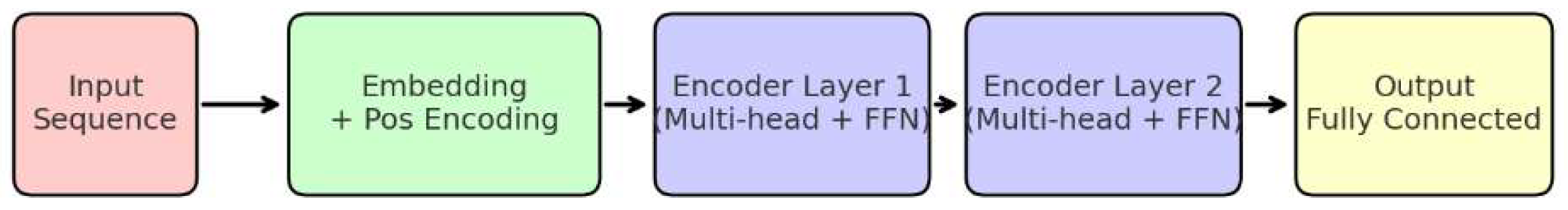
In our prediction problem, we are dealing with a regression task on a univariate time series (daily borrowing counts), rather than sequence-to-sequence generation. In this setting, the decoder part of the Transformer (which is used for autoregressive output generation) is not necessary – a sufficiently deep encoder can learn the sequence representation for forecasting the next value. Therefore, we base our model solely on the Transformer’s encoder component. Each encoder layer contains two main sublayers (with residual connections around each): a multi-head self-attention sublayer and a position-wise feed-forward network (FFN) sublayer. Layer normalization is applied after each sublayer’s residual addition to stabilize and speed up training [11]. The residual connections help prevent gradient degradation in deep models. Through these mechanisms, the encoder can capture complex and long-term temporal dependencies present in the borrowing data.
In our implementation, the input to the model is a sequence of historical borrowing counts with a certain window length (to be determined empirically). We first normalize these values (e.g., min-max scaling to [0, 1]) so that the model can train effectively. The input sequence is then passed through an embedding layer [12], which projects the scalar input at each time step into a higher-dimensional vector space (we use an embedding dimension of 32).
We add positional encoding to these embeddings to provide the model with information about the position of each time step in the sequence, since the Transformer has no inherent notion of sequence order without this addition. The sequence is then fed into a stack of Transformer encoder layers. We employ encoder layers (in our experiments or ) and each uses attention heads in the multi-head attention mechanism (with tested between 3 and 5). The multi-head self-attention allows the model to attend to multiple patterns or relationships in the sequence concurrently, effectively capturing both short-term and long-term dependencies. The feed-forward sublayer in each encoder further transforms and refines the features [13,14,15,16]. We found that using 2 encoder layers and 5 attention heads gave the best performance (as discussed in the Experiments section). The output from the final encoder layer is a high-dimensional representation capturing the sequence’s features; this is passed through a fully connected output layer to produce the final prediction (a single scalar which is the forecasted borrowing volume for the next day).
2.2. Loss Function and Optimizer
For training the model, we use a standard regression loss, the Mean Squared Error (MSE), which directly measures the average squared difference between the predicted values and the true values. The loss function is given by:
where is the number of samples in a batch, is the actual borrowing volume for sample , and is the model’s predicted volume. A smaller MSE indicates better model performance. During training, we typically use the square root of MSE (RMSE) as one of our evaluation metrics for interpretability, as it has the same unit as the original data, and we also use the Mean Absolute Error (MAE) metric (defined later) for additional evaluation.
We train the network using the Adam optimizer, which is an adaptive gradient descent method. Adam automatically adjusts the learning rate for each parameter and incorporates momentum terms for acceleration. This optimizer is well-suited for deep learning models as it tends to converge faster and more reliably. Specifically, Adam’s adaptive learning rates and momentum help to reduce oscillations during training and improve stability, while its bias-correction mechanism ensures more accurate updates in early training stages. These characteristics have made Adam a popular choice and it worked well for our Transformer model.
3. Experiments
3.1. Dataset and Data Preprocessing
We evaluated our approach on a dataset consisting of daily borrowing counts from a university library over several years [17]. The dataset contains 1583 daily records, reflecting fluctuating usage patterns over time. The overall trend of the data is nonlinear and exhibits clear periodic variations (e.g., weekly cycles and seasonal effects) along with irregular fluctuations. For example, weekends typically show noticeable drops in borrowing activity, while certain weekdays (like Wednesdays) may have peak usage, and there are higher peaks at the beginning and end of academic semesters. To use these data for supervised learning, we first normalized the borrowing volumes to a 0–1 range (to eliminate scale differences and speed up training).
We then applied a sliding window method to construct the training and test samples from the time series. A window of length $n$ days of past data is used to predict the borrowing volume of the next day. In our experiments, we determined the window size empirically and found that using the past 10 days as input provided a good balance between capturing short-term trends and model complexity. Using $n=10$ on the 1583-length series yields 1573 sequences (each 10-day input with its next-day target). We formed the dataset such that when the sliding window moves by one day, a new sequence–target pair is generated. We then split these sequences into a training set and a test set: the first 80% of the sequences (1258 samples) were used for training, and the most recent 20% (315 samples, roughly the last 45 weeks of data) were held out for testing and evaluation. The training set covers earlier years of data to train the model, while the test set represents a later period (not seen during training) to evaluate predictive performance on new data [18,19,20].
3.2. Evaluation Metrics
To assess the prediction accuracy, we use two common error metrics: Root Mean Square Error (RMSE) and Mean Absolute Error (MAE). The RMSE is defined as the square root of the average squared error:
where $N$ is the number of predictions, $y_i$ are actual values and $\hat{y}_i$ are predicted values. Meanwhile, MAE is the mean of absolute errors:
Both metrics measure the deviation of predictions from true values, with RMSE penalizing large errors more strongly (due to squaring) and MAE providing a linear measure of average error magnitude. Lower values of RMSE and MAE indicate better predictive performance.
3.3. Experimental Setup
We implemented the model in Python using PyTorch 2.3.1. Training was conducted on a workstation with an Intel Core i7-9700K CPU, an NVIDIA GeForce GTX 1070 GPU, and 16 GB RAM, running Windows 10. For fair comparison, we evaluated three baseline models against our Transformer: a GRU network, an LSTM network, and a Support Vector Regression (SVR) model. All neural network models (Transformer, GRU, LSTM) were trained with the Adam optimizer. We performed hyperparameter tuning for each model to ensure it was optimized for the task. For our Transformer model specifically, we conducted experiments to determine the best configuration of encoder layers and attention heads, as described below.
4. Results and Analysis
Hyperparameter Selection: We first carried out a series of experiments to find the optimal number of encoder layers and attention heads for the Transformer model. We tested configurations with and , resulting in 6 combinations of . In all cases, the input window size was fixed at 10 days. Each configuration was trained and evaluated on the same dataset, and to mitigate random fluctuations, we repeated each experiment 3 times and took the best result for comparison. Table 1 summarizes the performance (RMSE and MAE on the test set) for each configuration. We observed that the Transformer with 2 encoder layers and 5 attention heads achieved the lowest error (highlighted in the table). This configuration yielded an RMSE of 0.0562 and MAE of 0.0370 on the test set, outperforming the other combinations by a noticeable margin. Increasing the number of encoder layers to 3 did not improve performance further; in fact, certain 3-layer configurations had slightly higher error, possibly due to overfitting or the added complexity not being necessary for this dataset. Thus, we selected 2 layers and 5 heads as the Transformer model’s architecture for the subsequent comparisons.
Table 1. Impact of encoder layers and attention heads on Transformer performance (lower is better for errors).
Comparison with Baselines: Next, we evaluated the best-performing Transformer model against the baseline models (GRU, LSTM, and SVR) on the test set. Table 2 presents the test RMSE and MAE for each model. The Transformer clearly outperforms the other approaches on both metrics. In particular, the Transformer achieved an RMSE of 0.0565 and MAE of 0.0370, which is substantially lower than the errors of the GRU, LSTM, and SVR models.
Compared to the best deep learning baseline (LSTM), our Transformer reduced the RMSE by 16.2% and the MAE by 23.2%. Against the GRU, the improvements were even larger (approximately 19.3% lower RMSE and 20.6% lower MAE). Notably, the Transformer also outperformed the traditional SVR method by a wide margin, achieving about 18.1% lower RMSE and 35.4% lower MAE than SVR. These results underscore the advantage of the Transformer’s ability to capture complex temporal patterns through multi-head attention and global sequence representation. The Transformer model can attend to seasonality and irregular patterns (such as the weekly usage dips on weekends, mid-week peaks, and semester-start/end surges) within a single framework. In contrast, the LSTM and GRU, lacking an explicit attention mechanism, struggled to model these patterns as effectively.
To better understand the models’ predictions, we plotted the predicted vs. actual borrowing volumes on the test set for each model (Figure 2). The true borrowing counts exhibit considerable variability, including sharp peaks and troughs corresponding to the patterns mentioned above. We find that the LSTM’s prediction curve is overly smoothed – it fails to reach the high peaks or low valleys of the actual data, resulting in significant errors at critical points. The GRU model’s predictions, while capturing some fluctuations, tend to deviate from the actual values in multiple stretches; in particular, the GRU consistently overestimates the borrowing volume during certain periods. In contrast, the Transformer model’s predictions closely track the actual values and capture the amplitude of fluctuations more accurately, without the persistent bias observed in GRU’s output. The Transformer’s predicted line stays within the range of the true values and aligns well with the actual trend, demonstrating its superior ability to fit the data dynamics.
5. Conclusion
Insufficient parameter density resulted in significant reductions in output quality. Conversely, beyond a threshold, increasing density did not yield additional improvements, indicating a saturation effect. In practical applications, other external factors (e.g., mechanical disturbances, system noise, or random shocks) may also influence outcomes, highlighting the need to ensure robust parameterization when deploying the model.
In this study, we investigated a Transformer-based approach for predicting library book borrowing volumes. The proposed model leverages the Transformer encoder’s multi-head self-attention mechanism to effectively capture long-term and nonlinear dependencies in the borrowing time series, overcoming limitations of traditional RNN-based models. Our experimental results on a real-world library dataset demonstrated that the Transformer model achieves significantly lower error (in terms of RMSE and MAE) than benchmark models like GRU, LSTM, and SVR. For instance, the Transformer’s RMSE was 16.2% lower than that of an LSTM under optimal settings, and its MAE was 23.2% lower, indicating a substantial improvement in prediction accuracy. Qualitatively, we observed that the Transformer’s predictions adhere closely to actual usage patterns and reflect important fluctuations (such as weekly and seasonal effects), whereas the LSTM and GRU struggled with over-smoothing or bias in certain periods.
These findings highlight the Transformer model’s potential for time-series forecasting in the library context. By capturing complex patterns and adapting to dynamic changes in user behavior, a Transformer-based system could enable library management to better anticipate demand and optimize resource allocation (such as staffing or inventory of popular books). In future work, we plan to further refine the model – for example, by exploring optimization of hyperparameters (learning rates, deeper layers or different head configurations) and incorporating additional exogenous factors (holidays, special events, etc.) that might influence borrowing behavior. We will also consider expanding the model to predict multiple steps ahead or to other related metrics. Overall, our results suggest that Transformer architectures offer a promising avenue for improving the accuracy and robustness of library usage predictions, contributing to more intelligent and data-driven library services.
Funding
This research was funded by the Science Foundation of Shandong Province.
Conflicts of Interest
The authors declare no conflict of interest.
References
- Wen, Qingsong, et al. “Transformers in time series: A survey. arXiv 2022, arXiv:2202.07125.
- Wu, Haixu, et al. “Autoformer: Decomposition transformers with auto-correlation for long-term series forecasting.”. Advances in neural information processing systems 2021, 34, 22419–22430.
- Zhou, Haoyi, et al. “Informer: Beyond efficient transformer for long sequence time-series forecasting.”. Proceedings of the AAAI conference on artificial intelligence 2021, 35.
- Lim, Bryan, et al. “Temporal fusion transformers for interpretable multi-horizon time series forecasting.”. International journal of forecasting 2021, 37.4, 1748–1764.
- Sun, Shenwei et al. “Research on the Application of AI Code Assistants in C Language Programming Courses.”. 2025 7th International Conference on Computer Science and Technologies in Education (CSTE) 2025, 20–24.
- Huang, Yulin, et al. “Statistical Analysis on the Book Borrowing Quantity of University Library—Taking Qilu University of Technology as an Example.”. In 2020 6th International Conference on Social Science and Higher Education (ICSSHE 2020); Atlantis Press, 2020.
- Vrabková, Iveta, and Václav Friedrich. “The productivity of main services of city libraries: Using the example from the Czech Republic and the Slovak Republic.”. Library & Information Science Research 2019, 41.3, 100962.
- Sun, Jinbao. “Prediction and estimation of book borrowing in the library: Machine learning.”. Informatica 2021, 45, 1.
- Foo, Zhi-Yao, Kok-Why Ng, and Su-Cheng Haw. “Analysis of Book Preferences Among Visitors in Library System.”. TEM Journal 2024, 13, 1.
- Cao, Zhihao, et al. “Why does strawberry fruit weight distribution show positive skewness? A simulation model reveals the underlying processes of fruit production.”. Frontiers in Plant Science 2023, 14, 1255724. [CrossRef] [PubMed]
- Irani, Habib, and Vangelis Metsis. “Positional encoding in transformer-based time series models: a survey. arXiv 2025, arXiv:2502.12370.
- Shen, Li, and Yangzhu Wang. “TCCT: Tightly-coupled convolutional transformer on time series forecasting.”. Neurocomputing 2022, 480, 131–145. [CrossRef]
- Maldonado-Cruz, Eduardo, and Michael J. Pyrcz. “Multi-horizon well performance forecasting with temporal fusion transformers.”. Results in Engineering 2024, 21, 101776. [CrossRef]
- Liu, Xinhe, and Wenmin Wang. “Deep time series forecasting models: A comprehensive survey.”. Mathematics 2024, 12.10, 1504.
- Cao, Zhihao, et al. “Effects of bee density and hive distribution on pollination efficiency for greenhouse strawberries: A simulation study.”. Agronomy 2023, 13.3, 731.
- Cao, Zhihao, Shuo Jiang, and Hongchun Qu. “Strategies to enhance greenhouse strawberry yield through honeybee pollination behavior: a simulation study.”. Frontiers in Plant Science 2024, 15, 1514372. [CrossRef] [PubMed]
- Ahmed, Sabeen, et al. “Transformers in time-series analysis: A tutorial.”. Circuits, Systems, and Signal Processing 2023, 42.12, 7433–7466.
- Sommers, Alexander, et al. “A survey of transformer enabled time series synthesis.” 2024 IEEE 10th International Conference on Collaboration and Internet Computing (CIC). IEEE, 2024.
- Hyndman, Rob J., and Anne B. Koehler. “Another look at measures of forecast accuracy.”. International journal of forecasting 2006, 22.4, 679–688.
- Benidis, Konstantinos, et al. “Neural forecasting: Introduction and literature overview. arXiv 2020, arXiv:2004.10240.
Figure 2.
Actual vs. predicted borrowing volume on the test set for different models.
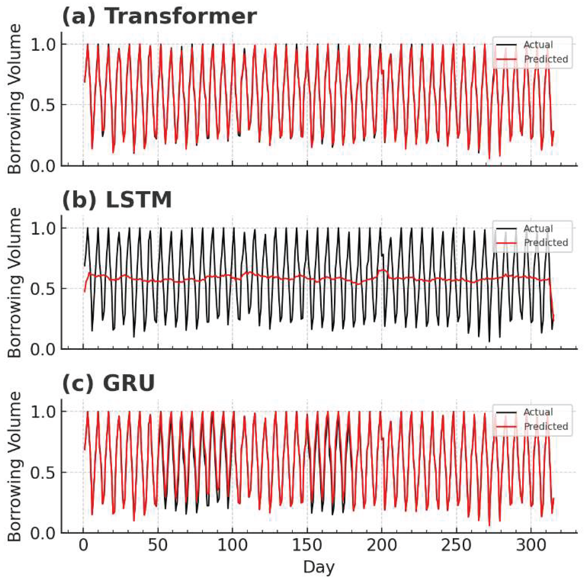

Table 1.
Impact of encoder layers and attention heads on Transformer performance.
| Encoder Layers | Attention Heads | RMSE | MAE |
|---|---|---|---|
| 2 | 3 | 0.0643 | 0.0503 |
| 2 | 4 | 0.0580 | 0.0405 |
| 2 | 5 | 0.0562 | 0.0370 |
| 3 | 3 | 0.0586 | 0.0391 |
| 3 | 4 | 0.0596 | 0.0412 |
| 3 | 5 | 0.0568 | 0.0389 |
Table 2.
Prediction error comparison of different models on the test set.
| Model | RMSE | MAE |
|---|---|---|
| GRU | 0.0700 | 0.0466 |
| LSTM | 0.0674 | 0.0482 |
| SVR | 0.0690 | 0.0573 |
| Transformer (ours) | 0.0565 | 0.0370 |
Disclaimer/Publisher’s Note: The statements, opinions and data contained in all publications are solely those of the individual author(s) and contributor(s) and not of MDPI and/or the editor(s). MDPI and/or the editor(s) disclaim responsibility for any injury to people or property resulting from any ideas, methods, instructions or products referred to in the content. |
© 2025 by the authors. Licensee MDPI, Basel, Switzerland. This article is an open access article distributed under the terms and conditions of the Creative Commons Attribution (CC BY) license (http://creativecommons.org/licenses/by/4.0/).
Copyright: This open access article is published under a Creative Commons CC BY 4.0 license, which permit the free download, distribution, and reuse, provided that the author and preprint are cited in any reuse.


