Submitted:
16 October 2025
Posted:
17 October 2025
You are already at the latest version
Abstract
Logistics has become an integral part of economic activity, with new formats such as front warehouses and hourly delivery demanding real-time visibility and rapid response. Minute-level road speed prediction is essential for platoon control, routing, and signal optimization, yet remains challenging due to heterogeneous and noisy data sources, highly coupled spatio-temporal interactions, and frequent distribution shifts. This paper proposes a Deep Operator Network–based framework that links logistics demand with traffic states. Warehouse and customer data are projected onto a five-kilometer subnetwork, generating six scenarios and about 1.2 million link–time samples. The proposed model decouples historical speeds in the branch from exogenous states in the trunk, allowing boundary changes to be incorporated as functional inputs rather than requiring retraining. Experiments demonstrate that the proposed method outperforms both classical regression and deep learning baselines, while ablation analyses verify robustness and interpretability. These findings establish operator learning as a promising direction for adaptive logistics forecasting.
Keywords:
logistics forecasting
; operator learning
; spatio-temporal modeling
1. Introduction
Short-term speed prediction, the task of forecasting vehicle or traffic speeds over brief future intervals, stands as a cornerstone technology for modern intelligent transportation systems and the advancement of autonomous vehicles [1]. With the rise of new formats such as front warehouses, community retail, local warehouses, and hourly delivery, the coupling between logistics and the national economy has become deeper, and the demand of supply chains for real-time visibility and rapid responsiveness has increased significantly. Smart logistics, supported by information technology, control techniques, optimization methods, and artificial intelligence, aims to reduce costs and increase efficiency across the entire chain through order allocation, vehicle management, route planning, and signal optimization [2]. To maintain stable operations and quickly recover from disruptions, road networks require predictability. Traffic forecasting [3], as a core capability, covers key quantities such as traffic states, road speeds, and travel times. Accurate prediction of states and speeds provides the basis for platoon control, route guidance, and signal optimization. Travel time prediction can serve as an early indicator for scheduling and coordination. In digital-twin-driven online simulations, forecasting further supports rolling evaluation and scenario selection. For safety and resilient operations, speed prediction also enables risk identification and early warning so that interventions can be made in high-risk spatio-temporal segments, reducing accidents and delays and ultimately improving punctuality and network reliability.
However, short-term road speed forecasting at the minute level faces multiple challenges in real environments. The first challenge lies in heterogeneity and noise at the data level. Vehicle operation data coexist with multi-source sensor data, where missing values, measurement errors, and irregular sampling are common. Spatial coverage of the sensing network is uneven, being dense in central urban areas but sparse in suburban regions, which results in coverage gaps and biased measurements. The second challenge is the complexity of spatio-temporal coupling. Traffic data simultaneously contain static structures and dynamic evolution, and cross-scale dependencies as well as nonlinear interactions are prominent. Deep learning has advanced spatiotemporal prediction by learning expressive, data-driven representations. Recent graph and sequence models capture spatial diffusion and temporal dependencies and have improved traffic flow and speed forecasting [4]. The third challenge is nonstationarity and distribution shift. Conventional neural predictions map vectors to vectors and typically require retraining or heavy fine-tuning when exogenous or boundary conditions change. Demand fluctuations, incidents, weather conditions, as well as changes in road networks and timetables occur frequently. These changes make models trained under previous conditions prone to mismatch in new scenarios, and the cost of maintenance and retraining remains high. Consequently, there is a need for modeling paradigms that can explicitly incorporate boundary changes at the input level while maintaining stable accuracy and lower maintenance costs when scenarios change.
To address these challenges, this study proposes a short-term road speed forecasting framework that directly connects logistics data with traffic prediction. To the best of our knowledge, no prior research has systematically mapped supply chain information such as warehouse and customer locations or dynamic demand volumes into traffic speed prediction while simultaneously applying operator learning [5] to achieve cross-scenario transferability. We conduct an initial exploration in this direction by projecting logistics demand and warehouse allocation onto the road network, creating learnable boundary conditions, and then applying an operator-learning approach to map historical sequences and contextual information to the next-step speed. This provides a new perspective for building a bridge between supply chain systems and traffic systems. At the data level, we build a unified data and evaluation pipeline that performs alignment, validity checks, anomaly removal, and feature standardization. We then split the data into training, validation, and test sets according to different scenarios, allowing us to evaluate the robustness of the model under diverse boundary combinations. At the modeling level, we adopt a branch–trunk design. The branch network encodes historical speed sequences of each link to capture short-term dynamics. The trunk network encodes contemporaneous exogenous and boundary states such as inflow, outflow, density, occupancy, waiting time, and travel time, which represent congestion intensity and downstream constraints. Multiplicative coupling of the two creates a mapping from functions to functions, enabling boundary changes to enter the inference process through input variation and thus maintaining accuracy while reducing retraining requirements when scenarios change.
We build six Simulation of Urban MObility (SUMO) [6] simulation scenarios, S001–S006, based on a five-kilometer urban subnetwork, with a time step of 60 seconds to output link-level data. These scenarios are driven by the Solomon dataset and vary in random seeds, total trip volumes, and order–warehouse allocation strategies. Such differences generate distinct origin–destination(OD) combinations, which describe the paired relationships between origins and destinations, their strengths, and their temporal distributions. They also include order quantities, vehicle counts or trip numbers, departure times, and service time windows for each pair. Different OD combinations determine the spatial and temporal distributions of inflows and outflows across the road network, which in turn shape congestion patterns and boundary conditions, leading to varying levels of prediction difficulty and transfer challenges. For all scenarios, we extract speed, inflow, outflow, density, occupancy, waiting time, and travel time. Inputs are constructed from twelve-step historical speeds together with six contemporaneous context features, and the next-step speed is used as the supervisory signal. After validity checks and anomaly filtering, approximately 1.19 million edge–time samples remain. To evaluate cross-scenario transfer, we use S001–S004 for training and validation and hold out S005–S006 as unseen test sets. Within the visible scenarios, we apply an 80/20 temporal split to ensure leakage-free evaluation that covers a variety of boundary conditions. To quantify the benefits of the proposed approach in modeling nonlinearities and history–context interactions, we systematically compare it with Ridge regression, multilayer perceptron (MLP), long short-term memory networks (LSTM), and temporal convolutional networks (TCN). We further conduct ablation studies to verify the necessity of trunk-side exogenous variables and perform counterfactual perturbations of these variables to illustrate the sensitivity and robustness of the model to congestion transitions. Results show that the proposed design alleviates feature bias caused by heterogeneous and noisy data, improves adaptability to distribution shifts, and enhances the representation of complex spatio-temporal interactions. Challenges such as missing-data handling, explicit spatial coupling, and uncertainty quantification are discussed in the limitations and left for future research.
The contributions of this paper are summarized as follows:
- This work constructs a unified logistics–traffic dataset by integrating Solomon demand data with SUMO-generated link-level states, producing about 1.2 million edge–time samples under six distinct scenarios, which provides a reproducible basis for cross-scene forecasting research.
- We propose a Deep Operator Network–based framework that decouples historical speeds through a branch network from contemporaneous exogenous and boundary states through a trunk network, enabling boundary changes to be incorporated as functional inputs rather than requiring frequent retraining.
- This paper conducts systematic evaluations and diagnostic analyses, showing that the proposed method outperforms both classical regression and deep learning baselines, while ablation and counterfactual experiments confirm the necessity of exogenous features and demonstrate robust and interpretable responses to congestion transitions.
- This work establishes a reproducible modeling and evaluation pipeline that links logistics demand with traffic forecasting, offering a foundation for adaptive control, predictive routing, and resilient logistics operations.
The rest of the paper is organized as follows. Section 2 reviews related work in logistics forecasting, traffic prediction, and operator learning. Section 3 describes the data design, feature construction, and the DeepONet architecture with training protocols. Section 4 presents results on cross-scene transfer, diagnostics, and ablations. Section 5 discusses implications for deployment, focusing on robustness, interpretability, and maintenance, and outlines limitations and future directions.
2. Related Work
Short-term speed prediction is not a monolithic concept. Its definition, particular the duration of the prediction of the prediction horizon, is highly dependent on the application context. The field is broadly divided into two categories: macroscopic traffic flow for forecasting and microscopic vehicle dynamics prediction. In this work, we focus on the former, which aims to predict aggregated traffic speed, which is typically the average speed of all vehicles on a specific road segment, over short horizons at the link or corridor level. This task is essential for traffic management, signal control, and route guidance. The prediction horizon in this context is generally in minutes, often ranging from 1 to 30 minutes [7]. In this work, the time interval for prediction is set to 1 minutes. The latter category focuses on individual vehicle trajectories and maneuvers over very short horizons and is crucial for autonomous driving and collision avoidance. The prediction horizons are up to 10 seconds [8] in this context.
2.1. Application of Deep Learning Method in Macroscopic Short-Term Speed Forecasting
Classical macroscopic speed forecasting methods include statistical models like ARIMA [9] and Kalman filters [10], which are effective for stationary regimes but limited in handling nonlinearity and dynamic boundaries. Simulation platforms like AnyLogic, FlexSim, and SUMO are widely used for prototyping and assessing operations, though they depend on calibration quality and face scalability challenges [11,12]. With ubiquitous sensing and digital infrastructure, deep learning has become a central paradigm for spatiotemporal prediction. Lana et al. [13] carried out joint feature selection and parameter tuning for short-term traffic flow forecasting based on heuristically optimized multi-layer neural networks. With the rapid development of deep learning, various neural network architectures have been proposed for traffic prediction tasks. Besides multi-layer perception(MLP),Convolutional Neural Network(CNN) and sequence models such as LSTM and TCN [14] are widely applied in time-series prediction tasks. Yang et al. [1] combined CNN and LSTM to predict the traffic speed in one region of Suzhou, illustrating better performance of their hybrid structure. Despite accuracy gains, many architectures remain brittle under distribution shift and require costly re–training when exogenous or boundary conditions like inflow or occupancy change.
A persistent challenge in macroscopic speed forecasting is transferability across scenes. Distribution shift, sparse sampling, and sensor noise degrade performance outside the training domain [15]. In traffic, models trained in one city or corridor often underperform in another without adaptation [16]. Domain adaptation techniques and adversarial alignment provide partial remedies but frequently entail substantial retraining and engineering overhead. Similar concerns arise in supply–chain forecasting [17]. Furthermore, the opacity of deep models complicates deployment in safety–critical logistics operations where auditability is required. These limitations motivate frameworks that can natively accommodate boundary variability and enable transparent analysis. Oerator learning [5], which maps functions to functions, offers a promising avenue to address these challenges.
2.2. Operator Learning in Scientific Machine Learning
Operator learning is supported by universal approximation theorem for operators [5,18]. A recurring theme is improved generalization under parametric and boundary changes, a property directly relevant to logistics where exogenous conditions evolve frequently. Operator learning emerged in scientific machine learning to directly approximate mappings between function spaces when classical vector-to-vector learning is inadequate for tasks such as partial differential equation solution operators, fractional operators, or control-to-state maps. Its mathematical footing extends universal approximation results from finite-dimensional functions to operators on compact subsets of Banach spaces. If an operator is continuous on a compact set of admissible inputs, then a suitably parameterized neural operator can approximate it uniformly on that set. This perspective justifies learning function-to-function maps rather than compressing all information into fixed-size vectors.
We consider an operator
where u may encode source terms, initial and boundary conditions, or control signals, and y denotes an evaluation location, e.g., spatial coordinates, time, or other query parameters. Training data are triples . To obtain a finite representation of the infinite-dimensional input u, choose sensor points and form
Operator learning parameterizes with two subnetworks and a bilinear fusion. The branch network encodes the input-function samples , and the trunk network encodes the query y. The prediction is
where p is the embedding dimension (interpretable as the rank of a low-rank expansion), and are the k-th components of the branch and trunk embeddings, and is an optional bias. This realizes the operator mapping by conditioning on u through the branch embedding and evaluating at arbitrary y through the trunk embedding, without requiring explicit convolutions or kernels; it therefore accommodates irregular geometries and unaligned samples. Extra context c, e.g., material or scenario parameters can be concatenated to the branch input, , or to the trunk input, .
The standard training objective of the operator is empirical risk minimization with mean-squared error:
where collects the parameters of g and f. When physics constraints are available, one may add a residual term in strong or weak form, for example
where encodes the governing operator in y and source q. This couples operator learning with physics-informed regularization.
After training, inference proceeds in two steps. Given a new input function , evaluate it on the same sensors to obtain and compute the branch embedding . For any collection of query locations y, compute and take the inner product:
Changing only recomputes the branch output; changing y only recomputes the trunk output, enabling cross-condition generalization and arbitrary-point evaluation. The trunk naturally accepts spatiotemporal queries by setting . For multi-output targets, one may append a small linear head from the scalar output to multiple channels, or use separate embeddings per channel.
Practical choices include the sensor count m in equation(2) where more sensors capture finer details of u but increase cost, the embedding rank p in equation(3) controlls expressive power, standardization or nondimensionalization of inputs, and lightweight MLP or residual blocks for both branch and trunk. Operator learning has demonstrated strong results across several domains: surrogate modeling for fluid and transport PDEs, fractional and integral operators, stochastic dynamics and filtering, control-to-state and model-predictive-control maps, and multi-physics responses. These successes highlight advantages in cross-condition generalization, handling irregular data, and enabling fast, arbitrary-point evaluations after offline training—properties that are directly useful for real-time macroscopic speed forecasting and decision support.
This work addresses link-level speed prediction at 60 s resolution to support traffic control and routing. We construct a framework that projects benchmark demand onto a 5 km urban subnetwork and generates microscopic traffic states, producing controlled yet realistic boundary variability for cross-scene transfer. We develop a branch–trunk factorization that disentangles short-history signals from exogenous and boundary context and demonstrate zero-retraining transfer on held-out scenes. We further provide diagnostic and counterfactual analyses that link accuracy gains to regime-consistent behavior and operational interpretability. To our knowledge, the combination of Solomon-driven demand, SUMO-based microscopic states, and operator learning for link-speed forecasting has not been previously reported.
3. Background and Problem Formulation
3.1. Motivation and Data Infrastructure for Macroscopic Short-Term Speed Forecasting
Short-horizon, link-level speed forecasts are both urgently needed and practically attainable. Public agencies seek to lower system-wide logistics costs via congestion mitigation and network reliability, while enterprises aim to reduce operating costs through improved transport scheduling, warehouse tasking, and production planning. These objectives are enabled by high-frequency data streams from loop detectors, video counters, GPS trajectories, and connected vehicles, together with platform-level integration of demand, inventory, production, and shipment records. This big-data infrastructure aligns public–private needs and supplies the covariates required for minute-scale forecasting in Intelligent Transportation Systems (ITS), supporting proactive signal control, dynamic speed limits, incident detection, reliable travel-time estimation, and predictive routing for freight [3]. At present, however, production datasets with the necessary spatial coverage, temporal resolution, and metadata are often inaccessible due to privacy and governance constraints, heterogeneous sensing deployments, missingness, and the difficulty of aligning exogenous and boundary conditions at scale. In this context, controlled data generation remains a practical and rigorous path. It enables reproducible experiments, systematic ablations, and conterfactual stress tests under well-specified distribution shifts. Looking ahead, continued advances in sensing, communications, and digital integration make it increasingly likely that such real-world data will be collected and shared in near-real time. Our study therefore develops and evaluates methods in advance of this capability, while using synthesized scenarios to ensure coverage, control and reproducibility.
We consider a 5 km urban subnetwork, defined as a contiguous district whose total centerline roadway length is approximately 5 km and that contains multiple signalized intersections and boundary inflow and outflow links. The choice of a 5 km scale is deliberate. It matches the control horizon of corridor- and district-level operations, e.g., coordinated signal control and variable speed advisories, where minute-resolution predictions are most actionable. Moreover, it is small enough to support reproducible, microscopic simulation with rich heterogeneity at manageable computational cost. It provides several boundary links so that exogenous inflow and outflow can vary across scenarios, which is essential for evaluating cross-scene transfer. Demand and customer attributes are taken from the Solomon benchmark and spatially assigned to network nodes, while traffic states are generated with the SUMO microscopic simulator under multiple scenarios [6,19]. In this research,signals are aggregated at interval s. Train, validation and test splits are performed by scenario to support cross-scene evaluation and to reflect distribution shift considerations [20].
Given a directed road network with edge set , SUMO outputs per-interval measurements for each edge , including mean speed , density, occupancy, counts of vehicles entering and leaving, average waiting time, and travel time [6,19]. These indicators summarize instantaneous traffic state and congestion intensity on each link. For each edge e and interval t, the goal is to predict the next-interval mean speed from a leakage-safe feature vector that combines short speed histories with contemporaneous exogenous variables:
with lag order and . The current-step speed appears only as the last element of the lagged history when forecasting —never as a contemporaneous feature for . Standardization is fit on the training scenarios and applied to validation and test to avoid leakage [21].
3.2. Formal Problem Statement and Model Overview
Let denote a predictor parameterized by . The one-step-ahead task is
We evaluate classical and neural baselines alongside an operator-learning model:
- Lag-1 persistence: , a naïve yet informative reference common in short-term time-series forecasting [22].
- Ridge regression: a linear baseline with -regularization, providing shrinkage and robustness to multicollinearity; we follow modern treatments and tuning practices [23].
- Multilayer perceptron (MLP): a feed-forward nonlinear predictor widely used in various scenarios [24].
- Operator learning: an operator-based predictor that maps function inputs to function outputs by factorizing the mapping into a branch network that encodes temporal history and a trunk network that encodes exogenous and boundary context, coupled multiplicatively by inner-product fusion to evaluate at arbitrary query points; we follow recent neural-operator formulations [27].
Architectural details, training protocols, and ablations are provided in the Methodology and Results sections.
4. Methodology
As illustrated in Figure 1, our methodology follows a three-stage pipeline: (i) data and scenario construction where Solomon demand instances are projected and simulated on a 5 km SUMO subnetwork to produce link-level edge states; (ii) feature engineering and dataset assembly that aligns, filters, and standardizes twelve-step speed histories together with contemporaneous exogenous and boundary covariates; and (iii) model learning and diagnostics using a branch–trunk Deep Operator Network that decouples short-term histories from contextual boundary inputs, followed by systematic cross-scene evaluation, ablations, and counterfactual perturbations.
4.1. Solomon Dataset as the Demand Prior
We ground the demand layer in the classical Solomon vehicle routing problem with time windows benchmarks [28,29]. The suite contains 56 instances with 100 customers, organized into six classes—C1, C2, R1, R2, RC1, RC2—where C/R/RC denote clustered, random, and mixed spatial layouts, and the “1” vs. “2” suffix reflects tighter vs. looser time windows, often implying a shorter vs. longer planning horizon. Each instance places 100 customers on a grid and follows a common schema: node index i, coordinates , demand , ready time , due date , and service duration ; the depot is node 0. File headers specify the fleet-size limit K and vehicle capacity Q. These fields map directly to our SUMO pipeline: coordinates are projected to the network coordinate reference system and snapped to the nearest nodes and edges; depot identifiers anchor origins; time windows drive release and service scheduling to produce temporally consistent origin-destination(OD) flows; and demands determine vehicle loading and trip counts. We use Solomon because its controlled spatial patterns and time-window tightness create diverse routing pressures and post-assignment congestion, which is essential for stress-testing forecasting models under heterogeneous boundary conditions.
4.2. Simulation Environment and Dataset Construction
We consider an urban subnetwork of approximately imported into SUMO, and instantiate six scenarios S001–S006 that vary random seeds and trip loads to diversify demand [6]. Beyond the static network, each scenario is parameterized by logistics demand and supply. Customer requests and depot locations shape OD patterns and temporal loading, which in turn drive the edge states observed during simulation. We ingest (i) customer planar coordinates which are projected to the network coordinate reference system, (ii) demand quantity with units or weight, (iii) requested service time windows , and (iv) depot or warehouse identifiers and coordinates. Orders are snapped to nearest edges and nodes and grouped into time buckets to form OD flows or discrete trips consistent with their time windows and depot assignments.
Given the OD specification, SUMO produces vehicle- and edge-level traces: (i) per-vehicle routes and traversed edge sequences, and, if needed, per-timestep positions; (ii) per-interval edge aggregates, inclluding speed, entered and left, density, occupancy, waitingTime, traveltime; and (iii) per-vehicle summaries. These outputs connect the logistics side, including who, when, from which depot to which customer, with how much load to the traffic side, including which edges are used, with what speeds and queues, enabling supervised learning on edge dynamics under realistic boundary conditions. Table 1 summarizes the data sources and their roles in linking logistics demand with traffic states.
From each edgedata, we extract per-edge, per-interval measurements {speed, entered, left, density, occupancy, waitingTime, traveltime}. We form supervised pairs where the input concatenates 12 speed lag () and 6 contemporaneous covariates as the context features above, yielding 18 inputs and scalar target of speed . The combined dataset has rows before filtering. To reduce artifacts, we retain rows satisfying validity checks for , nonnegative counts and finite speeds [6]. We exclude the current speed at time t from contemporaneous features to avoid leakage; only lagged speeds are used in inputs. Standardization is fit on training scenarios and applied to validation and test to prevent target or covariate leakage [21]. We split by scenario: S001–S004 supply training and validation, an 80/20 temporal split within each seen scene, and S005–S006 form the test set. The resulting sizes are , , .
4.3. Baseline Models
We compare (i) naïve persistence [22]; (ii) Ridge regression (L2-regularized linear model) on the 18-d input [23]; (iii) MLP on the same 18-d input, supported by modern universal-approximation results [24]; (iv) LSTM using the same 12-step window [30]; (v) TCN with dilated causal convolutions on the same 12-step window [31]. Unless noted, all models use identical splits and early stopping on validation [32]. All baselines consume the same feature set defined above to ensure parity.
- Ridge.
- We fit a linear model on :with features standardized using training statistics and intercept . The regularization is selected on a log-grid . Ridge offers a strong linear baseline with high inference throughput.
- MLP.
- Two hidden layers of width 256 with ReLU, dropout , Adam optimizer (), batch size 8192, up to 30 epochs; early stopping on validation.
- LSTM.
- We form a sequence where each step uses the k-th speed lag and the same exogenous context:yielding an input tensor . A single-layer LSTM (hidden size 128, dropout 0.1) processes the sequence; the last hidden state feeds a linear head to predict . Optimizer: Adam (), batch 8192, 30 epochs, early stopping.
- TCN.
- We use a causal Temporal Convolutional Network on the same sequence: four residual blocks with dilations , kernel size 3, 64 channels, dropout ; causal padding prevents leakage. The receptive field () covers the window. The block output is global-pooled and passed to a linear head. Optimizer and early stopping as above, and training hyperparameters in Table 2.
4.4. Operator-Learning Model
We model the one-step map from an edge’s recent speed history and its contemporaneous context to the next-step speed as a neural operator acting on two inputs: the 12-step lag vector and the 6-d context . Let and be branch and trunk embeddings. The prediction is their inner product in a p-dimensional latent space:
which realizes a low-rank factorization of the operator from to y [5,27]. Architecturally, both branch and trunk are MLPs with hidden width 256, dropout , and linear p-dimensional projections; we set . Optimization uses Adam with learning rate , batch size 8192, up to 30 epochs with early stopping on validation . All features are standardized using training statistics, and train/validation/test splits, random seeds, and library versions are fixed for reproducibility. The factorized form (9) decouples temporal history from exogenous conditions and enables counterfactual analyses without retraining: varying ,e.g., perturbing entered or density changes while keeping fixed, thus isolating the effect of boundary and context signals on . This branch–trunk inner-product realization exactly matches the DeepONet formulation for operator learning [5], so we henceforth refer to our model as DeepONet and use “DeepONet” to denote it throughout.
4.5. Evaluation
We report Mean Absolute Error (MAE), Root Mean Squared Error (RMSE), and :
In words, MAE reports the average absolute deviation in and is relatively robust to outliers; RMSE reports the quadratic mean error and emphasizes large deviations, which is desirable when large mistakes are particularly costly; and reports the proportion of variance explained relative to a mean-only baseline and can be negative if the model underperforms that baseline. Reporting de-standardized MAE and RMSE in enables operational interpretation, while facilitates scale-free comparison across scenes. All metrics are computed on de-standardized speeds (km/h) [21].
5. Experimental Results
5.1. Implementation Details
We first evaluate models under the leave-scenario-out protocol, trained on S001–S004 and test on the held-out scenes S005–S006 without retraining. All models use the inputs with 12 speed lags plus 6 exogenous trunk features and the same filtering. Metrics are computed on de-standardized speeds.Feature-wise standardization uses training-scene statistics only; test data are transformed with the same parameters. This protocol probes robustness to shifts in boundary and context conditions, e.g., demand intensity, time-window profiles, depot–customer configurations, rather than i.i.d. sample-level splits. Table 2 summarizes the final hyperparameters. All models are implemented in PyTorch 2.0.1 and trained on a single RTX 3060 GPU with 12 GB memory.
5.2. Leave-Scenario-Out Generalization Results
As shown by the leave-out evaluation in Table 3, operator learning delivers the strongest cross-scene transfer, achieving the second-best MAE of , the best RMSE of , and the highest of on the held-out scenes. The one-step persistence baseline performs poorly with MAE , RMSE , and , confirming that simply copying the last speed to the next step cannot accommodate demand shocks, congestion waves, or boundary-condition shifts across scenes. Linear ridge regression improves over persistence with MAE , RMSE , and , yet it remains far behind the deep models due to limited ability to capture nonlinear feature interactions and multiplicative effects between historical lags and exogenous inputs. Among deep baselines, the MLP, LSTM, and TCN all generalize without retraining but emphasize different error profiles. The LSTM attains lower pointwise errors than the MLP with MAE versus and RMSE versus , while its overall explained variance is lower with versus for the MLP. The TCN trails the LSTM with MAE , RMSE , and . Overall, Operator’s branch–trunk decomposition and multiplicative fusion better disentangle scene-level context from autoregressive signals, yielding consistently lower errors and higher under cross-scene shifts where boundary conditions change but lagged information remains informative.
5.3. Prediction Quality Analysis
We assess prediction quality using two diagnostics: parity plots from a random sample of points and error histograms that examine distributional tails. In the parity plots shown in Figure 2, the operator model tracks the line most closely across the full speed range, with a small and nearly homoscedastic spread, and panel titles report MAE, RMSE, and . The MLP, LSTM, and TCN also follow the diagonal but show increasing dispersion with speed, with under-prediction at the high end and over-prediction at the low end, indicating residual bias under higher loads. Ridge concentrates predictions in a narrow band due to regression to the mean, which lowers mid-range error but fails at extremes and produces near-vertical clouds. Persistence lies on the diagonal only when the signal is unchanged; once speed moves, errors increase sharply.
The error histograms in Figure 3 are consistent with these patterns. Persistence exhibits a tall spike at zero because many samples have no step-to-step change, so copying the last value is exactly correct in those cases, but large errors occur whenever dynamics are present, which explains its poor and sometimes negative in Table 3. Ridge produces a relatively narrow yet asymmetric distribution with heavy tails, reflecting shrinkage toward the mean rather than genuine dynamic modeling. In contrast, DeepONet residuals are both narrower and more symmetric among the learned models, indicating small and balanced errors across regimes and especially in medium-to-high load conditions. Overall, although trivial baselines can appear competitive in stationary slices, DeepONet achieves the best global generalization, with the lowest MAE and RMSE and the highest in Table 3, by capturing both level and slope over the full operating range. For completeness we also swap the roles, training on S005–S006 and testing on S001–S004, and the results show the same ranking.
5.4. Ablation Studies
We probe whether DeepONet’s gains arise from the branch–trunk factorization with multiplicative coupling rather than mere capacity. On the same held-out scenes as the main results, removing the trunk and using only the 12 lagged speeds — the branch-only variant — catastrophically degrades accuracy: MAE = 12.779, RMSE = 12.959, and . Relative to the full model with that attains MAE = 1.243, RMSE = 2.032, and , this corresponds to . The trunk therefore contributes indispensable exogenous context that the autoregressive footprint cannot infer. Panel a of Figure 4 summarizes the per-feature effects, and the complete numbers are reported in Table 4.
To quantify which context signals matter most, we drop each trunk feature in turn. Two variables dominate the degradation: removing density yields MAE = 20.193, RMSE = 38.480, and with , while removing traveltime yields MAE = 3.065, RMSE = 3.157, and with . Excluding entered or left produces moderate declines with and and and . Occupancy and waitingTime have smaller but non-negligible effects with and and and . These patterns align with traffic physics: density sets the operating regime on the fundamental diagram, traveltime calibrates congestion scale, and flow-balance signals refine local dynamics. The factorized operator exploits this structure, whereas a lag-only mapping cannot.
We also examine design sensitivity. A capacity-matched concatenation MLP on the same 18-dimensional input reaches MAE = 1.430, RMSE = 2.243, and , trailing DeepONet by RMSE and in as summarized in Table 4. Varying the latent width shows stable improvements without brittleness: yields MAE = 1.310, RMSE = 2.140, and ; yields MAE = 1.392, RMSE = 2.127, and ; yields MAE = 1.243, RMSE = 2.032, and . Panel b of Figure 4 visualizes this capacity sweep. Altogether, the evidence indicates that DeepONet’s advantage stems from disentangling temporal history in the branch and scene context in the trunk and combining them multiplicatively, rather than simply adding parameters.
5.5. Evidence for Operator Learning
We design tests that stress the conditional side of the problem—i.e., changes in exogenous and boundary features—where operator learning should excel.
To probe conditional behavior without retraining, we perform counterfactual perturbations of the trunk variables and measure the model response in Figure 5. For each feature we multiply its value by , , while keeping the lag sequence and all other context features fixed, and we plot the mean predicted speed across the test set. DeepONet exhibits responses that are monotone and physically plausible for the key variables: increasing density or traveltime lowers the predicted speed, whereas increasing net outflow raises it. The curves are smooth and show stronger, more elastic slopes than the concatenation MLP, indicating that DeepONet more faithfully captures how context conditions modulate the next-step mapping given the same history. Features with weak marginal utility in our ablations, such as waitingTime, show near-flat curves here as well, providing cross-consistency. The MLP displays flatter and occasionally less interpretable trends, e.g., a near-linear increase with entered, consistent with a model that averages effects in input space rather than learning a context-conditioned operator. The sharper, monotone, and stable DeepONet responses align with the drop-one ablation results where density and traveltime produced the largest degradation when removed, and they provide complementary evidence that the branch–trunk factorization with multiplicative coupling captures how exogenous conditions reparameterize the dynamics. As these curves are obtained with fixed weights, they directly reflect the learned operator rather than fine-tuning artifacts.
6. Conclusion
This study demonstrates that operator learning with a branch–trunk factorization is an effective and pragmatic approach for short-horizon, link-level speed forecasting in logistics settings. Across held-out scenes, the model consistently outperforms linear baselines and vector-to-vector neural networks while requiring little or no retraining under boundary variation—a critical property for operations subject to demand shocks, diversions, and schedule changes. By treating prediction as a map between function spaces, the method cleanly separates recent history from contemporaneous context, enables fast counterfactual queries,e.g., perturbing entered flow or travel time, and supports interpretable sensitivity analyses that connect numerical gains to regime-consistent behavior. However, Limitations remain. our evaluation uses a km simulated subnetwork, lacks explicit physics constraints, and covers a restricted portion of the function space. These gaps point to clear next steps—physics-informed losses, conservation, capacity, kinematic bounds, broader function-space pretraining followed by traffic fine-tuning, decision-centric and horizon-aware training in closed loop, richer exogenous features with calibrated uncertainty, and extensions from per-link predictors to spatial operators that capture upstream and downstream coupling. Together, these directions chart a pathway from accurate one-step forecasts to robust, decision-ready tools for real-world logistics networks.
Author Contributions
Conceptualization,Bin Yu.; methodology,Dawei Luo, Yong Chen; software, Bin Yu and Dawei Luo; validation, Bin Yu.; formal analysis, Bin Yu; investigation, Bin Yu and Dawei Luo; resources, Bin Yu; data curation, Bin Yu; writing—original draft, Bin Yu; writing—review & editing, Joonsoo Bae; visualization, Bin Yun; supervision, Bin Yu; project administration, Bin Yu. All authors have read and agreed to the published version of the manuscript.
Funding
This work was supported by the China Society of Logistics (CSL) Research Projects: (1) “Path Identification and Strategy for Digital Transformation in Small and Medium-sized Logistics Enterprises” (Grant No. 2025CSLKT3-083, 2025); (2) “Operation Workflow of Smart Factory Production Logistics and AGV Path Optimization” (Grant No. 2024CSLKT3-089, 2024).
Data Availability Statement
Simulation scripts and training code are available at [33].
Conflicts of Interest
The authors declare no conflict of interest.
Abbreviations
The following abbreviations are used in this manuscript:
| ADAM | Adaptive Moment Estimation (optimizer) |
| ARIMA | AutoRegressive Integrated Moving Average |
| DeepONet | Deep Operator Network |
| ITS | Intelligent Transportation Systems |
| LSTM | Long Short-Term Memory |
| MAE | Mean Absolute Error |
| MLP | Multilayer Perceptron |
| OD | Origin–Destination |
| PDE | Partial Differential Equation |
| ReLU | Rectified Linear Unit |
| RMSE | Root Mean Squared Error |
| SUMO | Simulation of Urban MObility |
| TCN | Temporal Convolutional Network |
| Coefficient of Determination |
References
- Yang, X.; Yuan, Y.; Liu, Z. Short-term traffic speed prediction of urban road with multi-source data. IEEE Access 2020, 8, 87541–87551. [Google Scholar] [CrossRef]
- Yuan, H.; Li, G. A survey of traffic prediction: from spatio-temporal data to intelligent transportation. Data Science and Engineering 2021, 6, 19–38. [Google Scholar] [CrossRef]
- Vlahogianni, E.I.; Karlaftis, M.G.; Golias, J.C. Short-term traffic forecasting: where we are and where we’re going. Transportation Research Part C: Emerging Technologies 2014, 43, 3–19. [Google Scholar] [CrossRef]
- Li, Y.; Yu, R.; Shahabi, C.; Liu, Y. Diffusion Convolutional Recurrent Neural Network: Data-Driven Traffic Forecasting. In Proceedings of the International Conference on Learning Representations; 2018. [Google Scholar]
- Lu, L.; Jin, P.; Pang, G.; Zhang, Z.; Karniadakis, G.E. Learning nonlinear operators via DeepONet based on the universal approximation theorem of operators. Nature Machine Intelligence 2021, 3, 218–229. [Google Scholar] [CrossRef]
- Krajzewicz, D.; Erdmann, J.; Behrisch, M.; Bieker, L. Recent Development and Applications of SUMO—Simulation of Urban MObility. International Journal On Advances in Systems and Measurements 2012, 5, 128–138. [Google Scholar]
- Yang, Z.; Wang, C. Short-term traffic flow prediction based on AST-MTL-CNN-GRU. IET Intelligent Transport Systems 2023, 17, 2205–2220. [Google Scholar] [CrossRef]
- Stockem Novo, A.; Hürten, C.; Baumann, R.; Sieberg, P. Self-evaluation of automated vehicles based on physics, state-of-the-art motion prediction and user experience. Scientific Reports 2023, 13, 12692. [Google Scholar] [CrossRef]
- Chatfield, C. Time-Series Forecasting; Chapman and Hall/CRC, 2000. [Google Scholar]
- Harvey, A.C. Forecasting, Structural Time Series Models and the Kalman Filter; Cambridge University Press, 1990. [Google Scholar]
- Chahal, K.; Eldabi, T. Simulation modelling for logistics and supply chain management: A literature review. Journal of Simulation 2013, 7, 14–24. [Google Scholar]
- Rojas, R.; Iglesias, J.; Mejia, G. Application of FlexSim in modeling and simulation of logistics processes. Procedia Engineering 2016, 149, 407–411. [Google Scholar]
- Laña, I.; Del Ser, J.; Vélez, M.; Oregi, I. Joint feature selection and parameter tuning for short-term traffic flow forecasting based on heuristically optimized multi-layer neural networks. In Proceedings of the International conference on harmony search algorithm; Springer, 2017; pp. 91–100. [Google Scholar]
- Lim, B.; Zohren, S. Time-series forecasting with deep learning: A survey. Philosophical Transactions of the Royal Society A 2021, 379, 20200209. [Google Scholar] [CrossRef] [PubMed]
- Subbaswamy, A.; Saria, S. Evaluating model robustness and stability to dataset shift. Proceedings of the IEEE 2021, 109, 802–825. [Google Scholar]
- Zhang, J.; et al. Transfer learning for traffic forecasting. In Proceedings of the IJCAI; 2019. [Google Scholar]
- Carbonneau, R.; Laframboise, K.; Vahidov, R. Application of machine learning techniques for supply chain demand forecasting. European Journal of Operational Research 2008, 184, 1140–1154. [Google Scholar] [CrossRef]
- Li, Z.; Kovachki, N.B.; Azizzadenesheli, K.; Liu, B.; Bhattacharya, K.; Stuart, A.M.; Anandkumar, A. Fourier Neural Operator for parametric PDEs. In Proceedings of the Proceedings of the International Conference on Learning Representations (ICLR); 2021. [Google Scholar]
- Chowdhury, M.M.H.; Chakraborty, T. Calibration of SUMO Microscopic Simulation for Heterogeneous Traffic Condition: The Case of the City of Khulna, Bangladesh. Transportation Engineering 2024, 18, 100281. [Google Scholar] [CrossRef]
- Quiñonero-Candela, J.; et al. Dataset shift in machine learning. In Proceedings of the MIT Press; 2009. [Google Scholar]
- Makridakis, S.; Spiliotis, E.; Assimakopoulos, V. Statistical and machine learning forecasting methods: Concerns and ways forward. PloS one 2018, 13, e0194889. [Google Scholar] [CrossRef] [PubMed]
- Hyndman, R.J.; Athanasopoulos, G. Forecasting: Principles and Practice, 3rd ed.; OTexts, 2021. [Google Scholar]
- James, G.; Witten, D.; Hastie, T.; Tibshirani, R. An Introduction to Statistical Learning, 2nd ed.; Springer, 2021. [Google Scholar]
- Shen, Z.; Yang, H.; Zhang, S. A Survey on Universal Approximation Theorems. arXiv 2024, arXiv:2407.12895. [Google Scholar] [CrossRef]
- Sutskever, I.; Vinyals, O.; Le, Q.V. Sequence to Sequence Learning with Neural Networks. In Proceedings of the Advances in Neural Information Processing Systems; 2014. [Google Scholar]
- Lim, B.; Zohren, S. Time Series Forecasting With Deep Learning: A Survey. arXiv 2020, arXiv:2004.13408. [Google Scholar] [CrossRef]
- Kovachki, N.; et al. Neural Operator: Learning Maps Between Function Spaces. Journal of Machine Learning Research 2023, 24, 1–97. [Google Scholar]
- Solomon, M.M. Algorithms for the vehicle routing and scheduling problems with time window constraints. Operations Research 1987, 35, 254–265. [Google Scholar] [CrossRef]
- Gunawan, A.; Kendall, G.; McCollum, B.; Seow, H.V.; Lee, L.S. Vehicle routing: Review of benchmark datasets. Journal of the Operational Research Society 2021, 72, 1794–1807. [Google Scholar] [CrossRef]
- Hochreiter, S.; Schmidhuber, J. Long short-term memory. Neural Computation 1997, 9, 1735–1780. [Google Scholar] [CrossRef]
- Bai, S.; Kolter, J.Z.; Koltun, V. An Empirical Evaluation of Generic Convolutional and Recurrent Networks for Sequence Modeling. arXiv 2018, arXiv:1803.01271. [Google Scholar] [CrossRef]
- Bai, Y.; Luo, J.; Jiang, Y.; Li, Z.; Xia, S.; Chen, H. Understanding and Improving Early Stopping for Learning with Noisy Labels. In Proceedings of the NeurIPS; 2021. [Google Scholar]
- jbnu55343. scm_deeponet: Simulation scripts and training code. https://github.com/jbnu55343/scm_deeponet, 2025. Accessed: 2025-10-03.
Figure 1.
Project workflow: from Solomon demand mapping and SUMO simulation, through feature construction and operator-style branch–trunk modeling, to cross-scene evaluation and diagnostics.
Figure 1.
Project workflow: from Solomon demand mapping and SUMO simulation, through feature construction and operator-style branch–trunk modeling, to cross-scene evaluation and diagnostics.
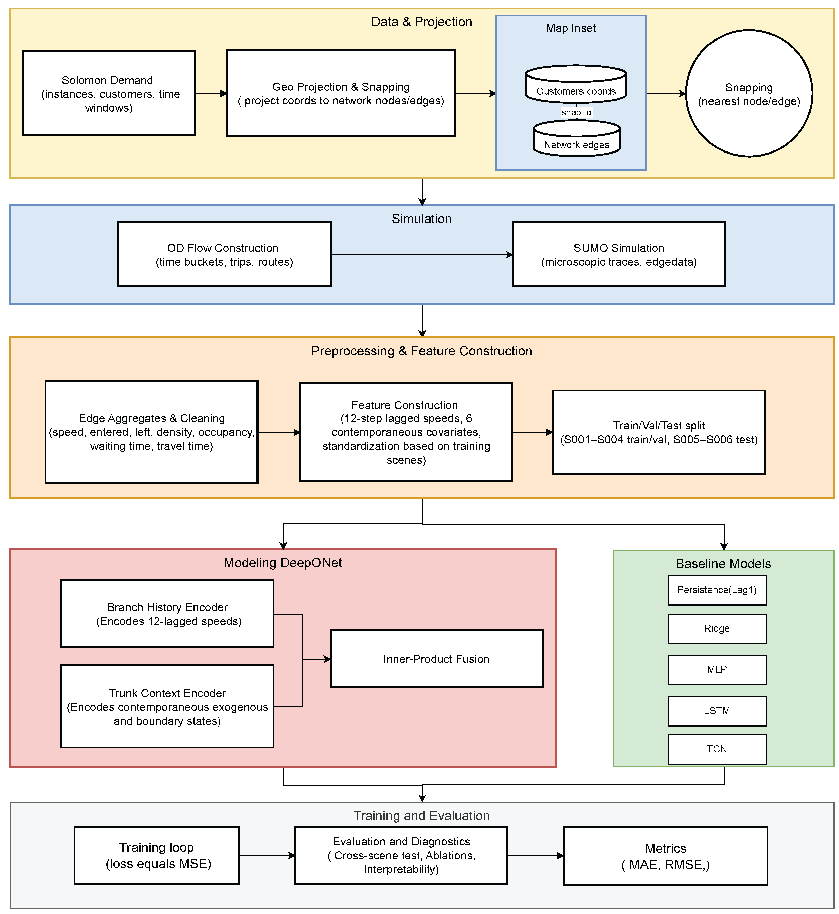
Figure 2.
Parity plots (random sample of points per model). Titles report MAE, RMSE, and . The diagonal denotes perfect agreement.
Figure 2.
Parity plots (random sample of points per model). Titles report MAE, RMSE, and . The diagonal denotes perfect agreement.
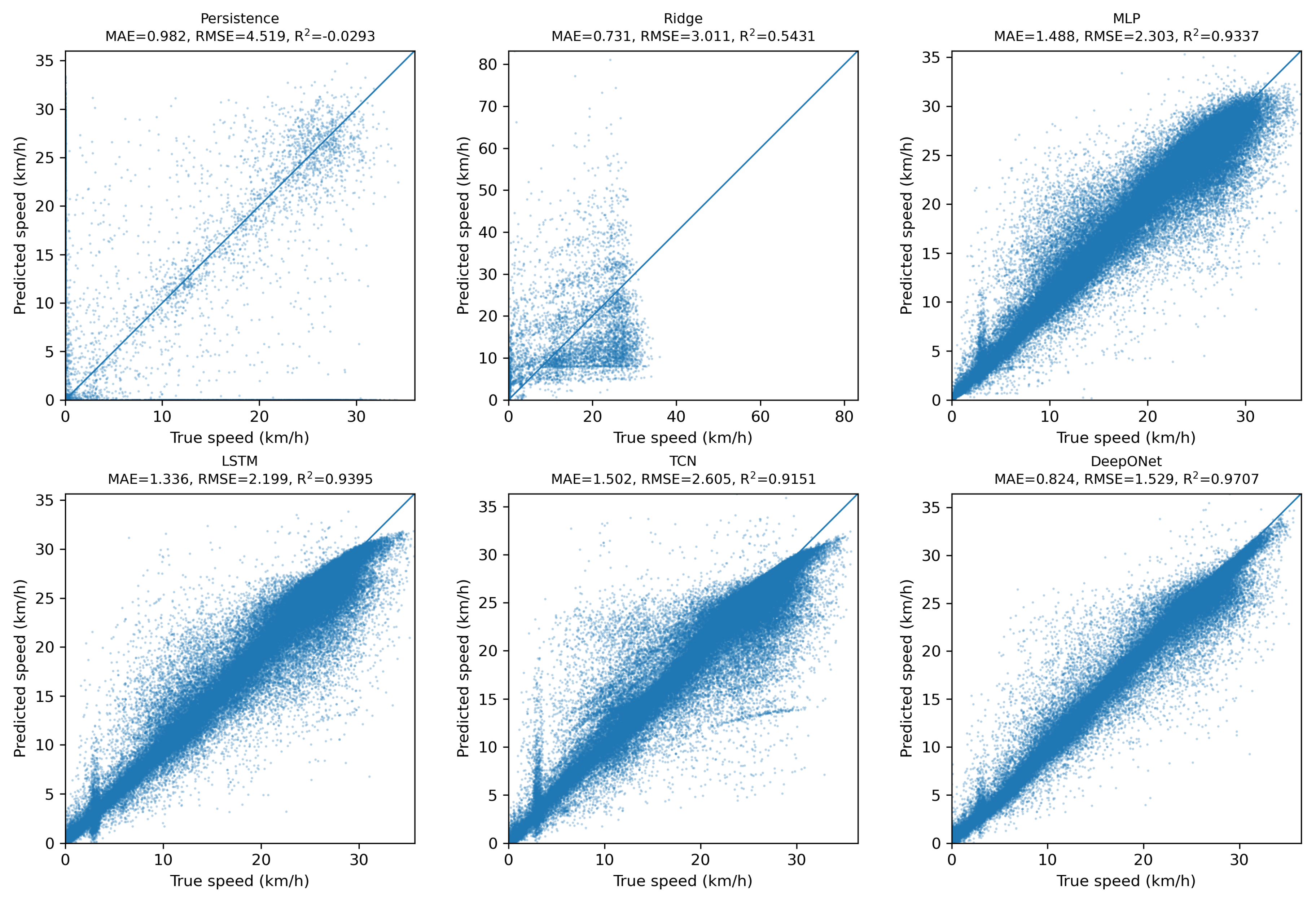
Figure 3.
Error histograms (predicted − true, km/h) for all models. Each panel shows the density of errors with a common x–axis range set by the 1–99% combined quantiles.
Figure 3.
Error histograms (predicted − true, km/h) for all models. Each panel shows the density of errors with a common x–axis range set by the 1–99% combined quantiles.
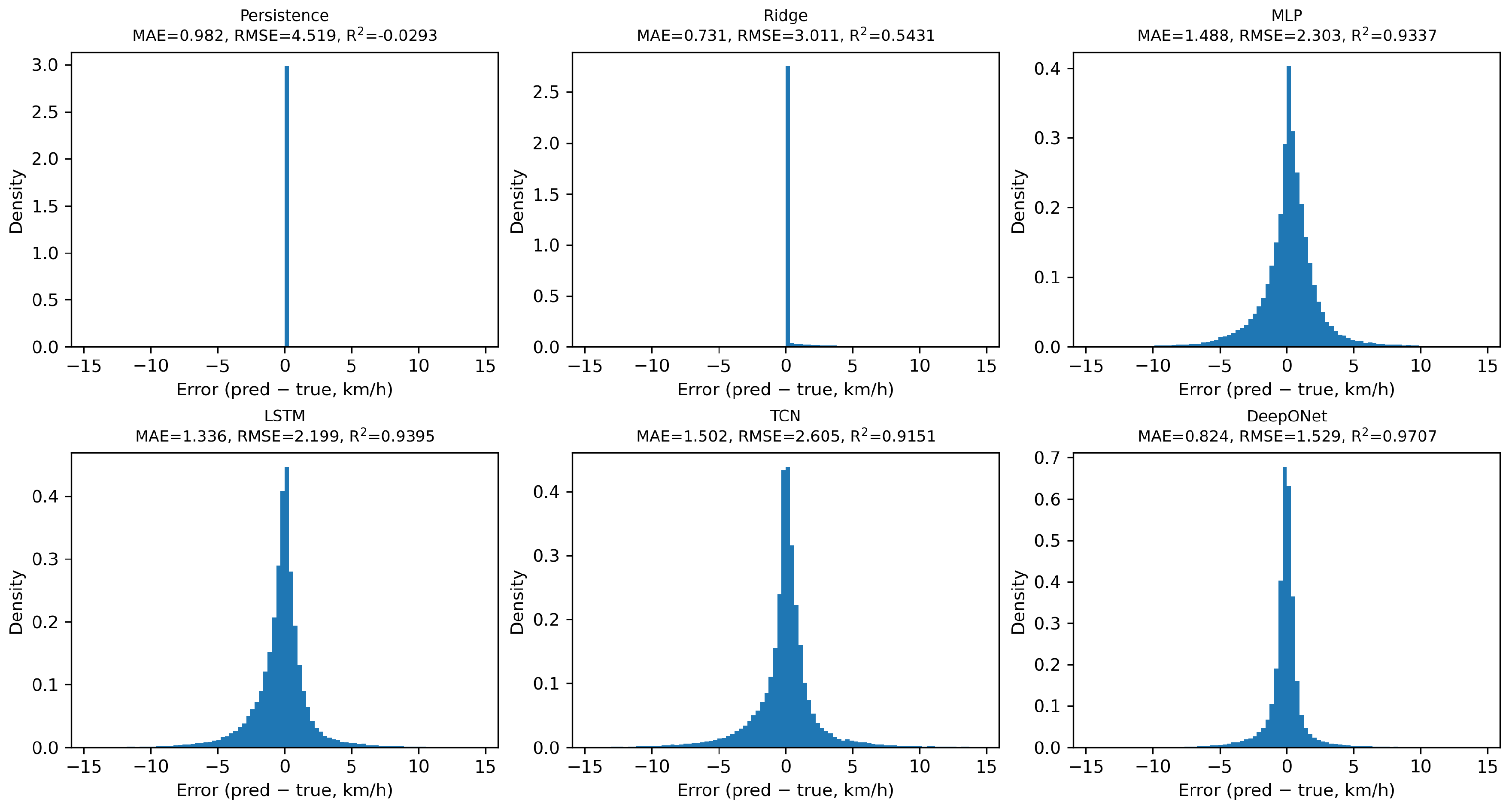
Figure 4.
Ablation diagnostics. Removing density or traveltime causes the largest degradation, confirming the value of exogenous context. Increasing latent width p steadily improves performance without brittleness.
Figure 4.
Ablation diagnostics. Removing density or traveltime causes the largest degradation, confirming the value of exogenous context. Increasing latent width p steadily improves performance without brittleness.
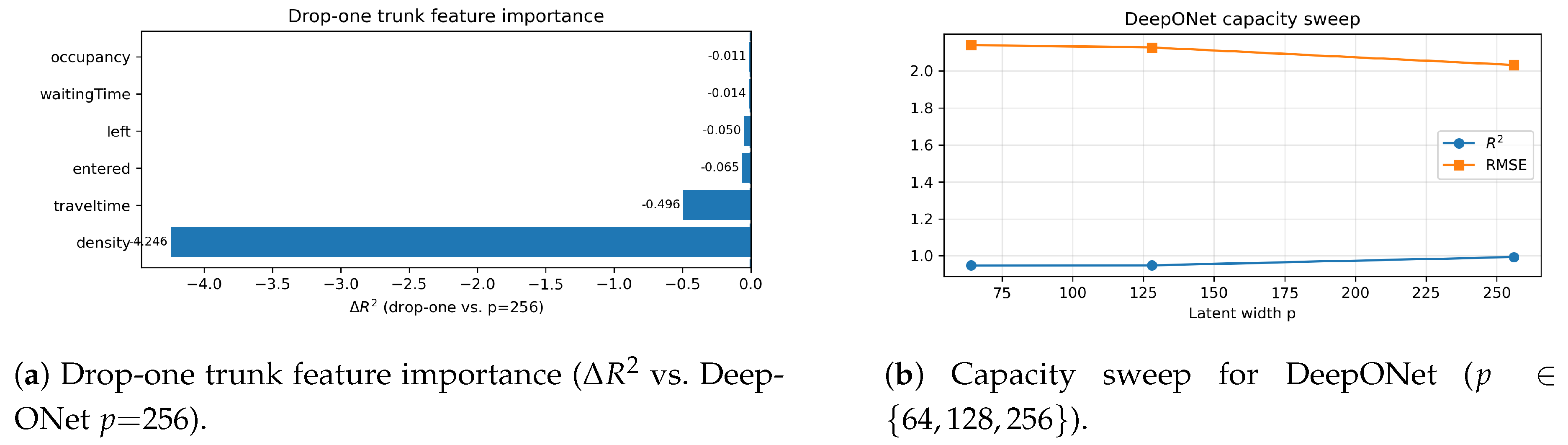
Figure 5.
Zero-retraining counterfactual responses to multiplicative perturbations of trunk features. For each feature , we evaluate the mean predicted speed after scaling that feature by with , holding all other inputs fixed. DeepONet (blue) and a concatenation MLP (orange) are compared.
Figure 5.
Zero-retraining counterfactual responses to multiplicative perturbations of trunk features. For each feature , we evaluate the mean predicted speed after scaling that feature by with , holding all other inputs fixed. DeepONet (blue) and a concatenation MLP (orange) are compared.
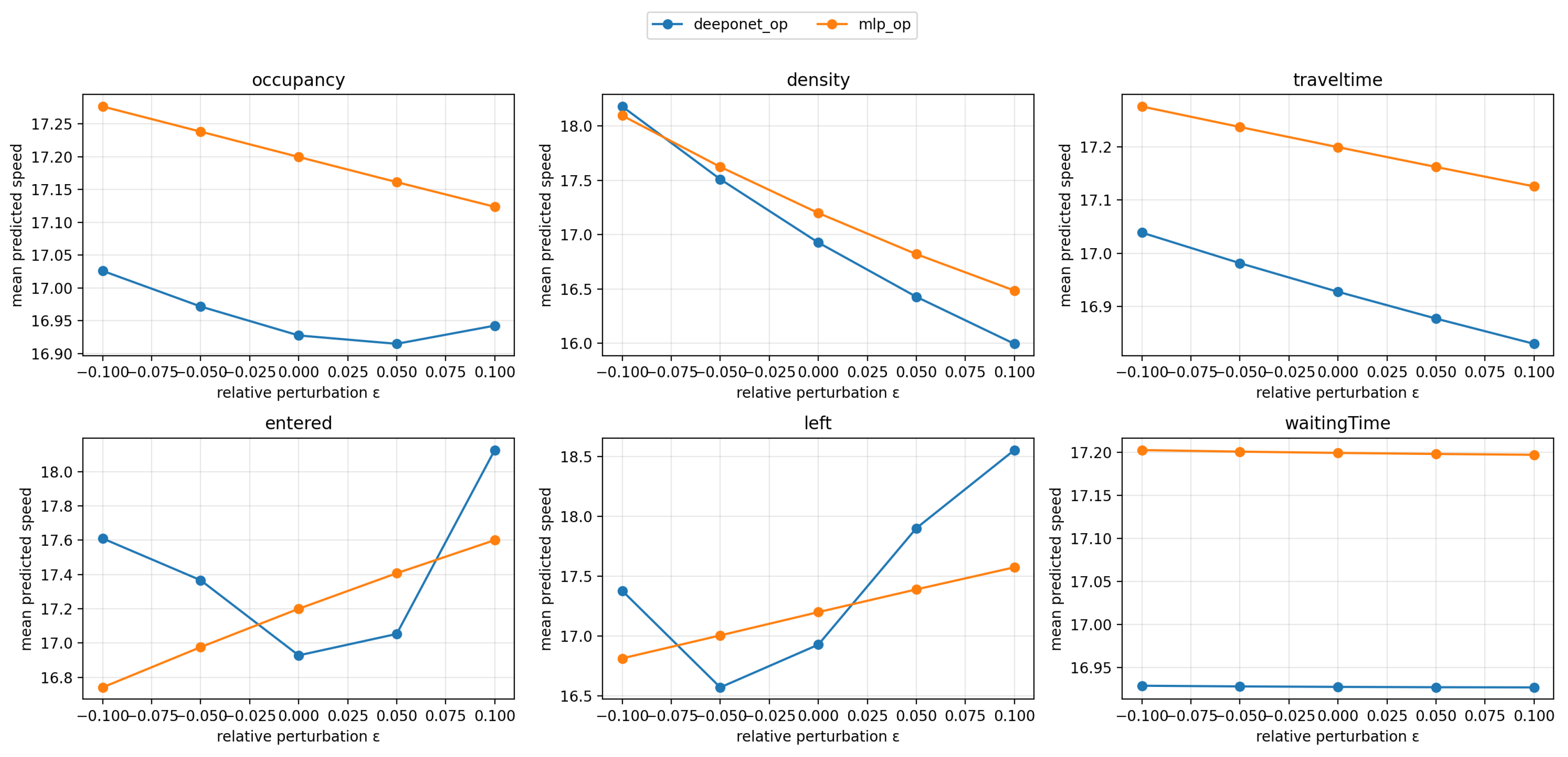

Table 1.
Data sources and logistics–traffic linkage.
| Layer | Fields | Usage |
|---|---|---|
| Demand (orders) | cust_id, , qty, , depot_id | Build OD flows/trips; snap to network; time-bucket by request; define boundary/context for scenes |
| Supply (depots) | depot coordinates; capacity (if available) | Define sources/sinks; origin assignment for orders |
| Routes (veh) | vehroutes.xml: edge sequences | Path reconstruction; edge utilization; optional node traversal via topology |
| Edge aggregates | edgedata.xml: speed, entered, left, density, occupancy, waitingTime, traveltime | Main supervised features/targets; per-interval edge-level learning |
| Vehicle summaries | tripinfo.xml: departures/arrivals; delays | Consistency checks; calibration/validation of OD temporal profiles |
Table 2.
Final training hyperparameters used in the study.
| Model | Input shape | Regularization | Optimizer & LR | Batch | Max epochs / ES |
|---|---|---|---|---|---|
| Persistence (lag1) | 18 (uses lag1 only) | — | — | — | — |
| Ridge | 18 | L2 ( tuned) | closed-form / LBFGS | N/A | N/A |
| MLP | 18 | Dropout | Adam, | 8192 | 30 / patience 5 |
| LSTM | Dropout | Adam, | 8192 | 30 / patience 5 | |
| TCN | Dropout | Adam, | 8192 | 30 / patience 5 | |
| DeepONet | Branch: 12; Trunk: 6 | Dropout | Adam, | 8192 | 30 / patience 5 |
Table 3.
Zero-retraining results on held-out scenes (S005–S006) after training on S001–S004. Best in bold, second-best underlined.
Table 3.
Zero-retraining results on held-out scenes (S005–S006) after training on S001–S004. Best in bold, second-best underlined.
| Model | MAE (km/h) | RMSE (km/h) | |
|---|---|---|---|
| Persistence (lag1) | 0.982 | 4.519 | -0.0293 |
| Ridge | 0.731 | 3.011 | 0.5431 |
| MLP (12 lags + exog.) | 1.430 | 2.243 | 0.9856 |
| LSTM (12 steps) | 1.293 | 2.130 | 0.9483 |
| TCN (12 steps) | 1.447 | 2.526 | 0.9273 |
| DeepONet () | 0.807 | 1.493 | 0.9936 |
Table 4.
Ablations on input configuration and architecture (held-out scenes).
| Configuration | MAE | RMSE | ||||
|---|---|---|---|---|---|---|
| DeepONet (Branch-only; 12 lags) | 12.779 | +11.536 | 12.959 | +10.927 | -7.4611 | -8.4547 |
| DeepONet - occupancy | 1.393 | +0.150 | 2.447 | +0.415 | 0.9828 | -0.0108 |
| DeepONet - density | 20.193 | +18.950 | 38.480 | +36.448 | -3.2520 | -4.2456 |
| DeepONet - traveltime | 3.065 | +1.822 | 3.157 | +1.125 | 0.4979 | -0.4957 |
| DeepONet - entered | 3.782 | +2.539 | 4.974 | +2.942 | 0.9289 | -0.0647 |
| DeepONet - left | 3.112 | +1.869 | 4.423 | +2.391 | 0.9438 | -0.0498 |
| DeepONet - waitingTime | 1.884 | +0.641 | 2.671 | +0.639 | 0.9795 | -0.0141 |
| DeepONet (p=64) | 1.310 | +0.067 | 2.140 | +0.108 | 0.9478 | -0.0458 |
| DeepONet (p=128) | 1.392 | +0.149 | 2.127 | +0.095 | 0.9484 | -0.0452 |
| DeepONet (p=256) | 1.243 | +0.000 | 2.032 | +0.000 | 0.9936 | +0.0000 |
| Concat-MLP (18-d) | 1.430 | +0.187 | 2.243 | +0.211 | 0.9856 | -0.0080 |
Disclaimer/Publisher’s Note: The statements, opinions and data contained in all publications are solely those of the individual author(s) and contributor(s) and not of MDPI and/or the editor(s). MDPI and/or the editor(s) disclaim responsibility for any injury to people or property resulting from any ideas, methods, instructions or products referred to in the content. |
© 2025 by the authors. Licensee MDPI, Basel, Switzerland. This article is an open access article distributed under the terms and conditions of the Creative Commons Attribution (CC BY) license (http://creativecommons.org/licenses/by/4.0/).
Copyright: This open access article is published under a Creative Commons CC BY 4.0 license, which permit the free download, distribution, and reuse, provided that the author and preprint are cited in any reuse.


